Light deflection in Observation: Angle differences between two null geodesics on the de Sitter spacetime with multi-lensing objects

Abstract

We derive angle differences between two null geodesics, propagating from light sources to an observer, on the de Sitter spacetime with multi-lensing objects. Assuming the lensing objects are mass monopoles on the de Sitter background, we derive the metric tensor by solving the Einstein equation perturbatively. On that spacetime, we solve a null geodesic parametrized by the coordinate time. Using the null geodesics, we define the angle differences in a coordinate invariant way. We take in the relativistic effects up to the first order of perturbation and clarify the magnitude of approximation errors. We find that the rest observer, who sees the isotropic cosmic space, implicitly observes the effect of the cosmological constant on the angle differences through the positions of the light sources. As a practical application, we regard the massive black hole at our galactic center (Sgr A*) and the solar system as the lensing objects, further a star and a flare around Sgr A* as the light sources. We write the angle differences between these light sources using their spatial coordinates. We find that deflections by Sgr A* remain in the angle differences while deflections by the solar system cancel out up to the first order of perturbation. The deflections by Sgr A* amounts around 10 microarcseconds, which is detectable in the near future observations.

I Introduction

Gravitational deflection of light is an important phenomenon predicted by the general relativity and/or other metric theories of gravity. When we treat a light or a massless particle just as a point and consider the gravitational force only, we express its path by a geometric straight line, that is, a null geodesic. To obtain a theoretical prediction for a path of light we observe, we need to solve the null geodesic analytically or numerically for a given geometry. The gravitational deflection of light is actually detected in a broad physical scale from the deflection by the sun firstly observed by Eddington Dyson:1920cwa to the gravitational lensing by the cluster of galaxies in the cosmological scale lensing . Among them, it is actively searched that how the cosmological constant affects the light deflection. Especially, with the use of the Gauss-Bonnet’s theorem, the deflection angle of light has been exactly defined Gibbons:2008ru and derived for the Schwarzschild-de Sitter(SdS) spacetime and so on Ishihara:2016vdc ; Ono:2019hkw ; Takizawa:2020egm .

In practical observations of the lights, we measure angle differences between the light rays entering the observer. Then, how do we derive the angle differences from the null geodesics traveling the present universe? The present universe is nearer to the de Sitter spacetime with multi lensing objects rather than the SdS spacetime. Thus, we should consider the spacetime where the lensing objects are put onto the de Sitter background as the first-order approximation of the real universe. This construction is similar to the Einstein-Infeld-Hoffman approximation where the astrophysical objects are put onto the Minkowski background perturbatively. Instead, we treat the lensing objects as the perturbation on the de Sitter background, as in the cosmological perturbation theory. We note that the de Sitter background referred to here expresses just a local part of the whole universe since by the lights from the astrophysical objects, we can measure the geometrical effect between the observer and those objects only. The local part of spacetime does not involve the whole of our Hubble patch filled by the cosmic microwave background (CMB).

Also, the actual observational data are obtained at the observer’s proper time. If we model the motion of the observer properly, it is not difficult to express the proper time by the coordinate time. So, it is useful to solve the null geodesic parametrized by the coordinate time for comparing to the observational data. This parametrization has a numerical advantage also since we do not need to solve the full geodesic equations but the spatial parts of it only.

In this article, we derive the angle differences between two light rays which travel in the de Sitter spacetime with multi lensing objects and enter an observer. We solve the spatial part of the null geodesic parametrized by the coordinate time and use it for the angle differences. We assume that all the lensing objects move slowly relative to the light speed and treat them as mass monopoles. This corresponds to the first order post-Newtonian approximation, and we treat the cosmological constant term in the metric as the perturbation also. For all the calculations, we treat the relativistic effect perturbatively and take into the leading order corrections with clarifying the magnitude of the approximation errors. For simplicity, we regard ourselves as a rest observer at the spatial origin in the static coordinate system. This observer sees the isotropic cosmic space and corresponds to the observer who sees the homogeneous and isotropic universe in the flat slicing of the de Sitter spacetime. We evaluate the angle differences between the light rays measured by this observer for a practical example.

This article is organized as follows. In Sec.II, we solve the null geodesic which travels from a light source to an observer. We expand the solution around a uniform linear motion and take the first-order corrections perturbatively. In Sec.III, we define the angle differences between two null geodesics in a coordinate independent way using the tetrad basis at the observer. We derive an approximate expression for small angle differences by using the apparent velocity of the lights derived in Sec.II. In Sec.IV, we apply our formula of the small angle differences to a practical example, in which we consider the solar system and the massive black hole at our galactic center (Sagittarius A*, Sgr A*) as the lensing objects. We express the deflections of lights by the spatial positions of the light sources and the lensing objects. We will find that the deflections by the solar system cancel out for the small angle differences and only the deflection by Sagittarius A* remains. Sec.V is devoted to a summary. We add three appendices. In App.A, we perform a coordinate transformation perturbatively from the usual static slice of the de Sitter spacetime to an isotropic slice. In App.B, we give a technical detail for the derivation of the angle differences. In App.C, we change the coordinate as boosting the rest observer to a moving observer and we confirm the coordinate invariance of the angle differences calculating in the two different coordinates. Throughout this article, we normalize the light speed to unity, $c=1$. The spatial components of physical quantities are denoted with arrows or the Roman indices. The dot between the quantities with arrows implies a contraction of their components.

II Null geodesics

We derive an explicit solution of null geodesic, propagating from a light source to a timelike observer, in the spacetime with multi-lensing objects and the cosmological constant. We consider a weak gravitational region only, so that we expand the spacetime perturbatively from the Minkowski spacetime. In addition, we assume that all the lensing objects are moving much slower than light and we ignore all of the multipole moments of the lensing objects.

In this set up, the energy-momentum tensor for slowly moving lensing objects is given as

$$T^{0}_{0} =-\rho,\ T^{i}_{0}\approx\rho v_{J}^{i},\ T^{i}_{j}\approx\rho v_{J}^{i}v_{Jj},$$

$$\rho \approx\sum_{J}M_{J}\delta^{3}(\vec{r}-\vec{r}_{J})\ ,$$ (1)

where $v_{J}^{i}$ and $M_{J}$ are the velocity and the mass of the lensing objects, respectively. $\vec{r}$ represents the spatial coordinate and $\vec{r}_{J}$ is the spatial coordinate of the $J$-th lensing objects. We consider the mass monopoles only for the energy density. In general relativity, the energy density of mass monopoles generates the gravitational potential treated as the first-order perturbation in the weak field region. The velocity $v_{J}^{i}$ of lensing objects is a small quantity also, and hence we cut off $T^{i}_{0}$ and $T^{i}_{j}$ as higher-order perturbations

$$T^{i}_{0}\approx 0,\ T^{i}_{j}\approx 0\ .$$ (2)

This approximation corresponds to the first order post-Newtonian (1PN) expansion.

Up to the first order of perturbative expansion, the metric has the following form:

$$ds^{2} =-(1+2\Phi(t,\vec{r}))dt^{2}+(1+2\Psi(t,\vec{r}))d\vec{r}^{2}\ ,$$

$$d\vec{r}^{2} :=dx^{2}+dy^{2}+dz^{2},$$ (3)

where we treat the Newtonian potential $\Phi$ and the curvature perturbation $\Psi$ perturbatively. Note that we have already fixed the gauge, so-called the Newtonian gauge. The vector and tensor perturbations are ignored since they are nothing more than the higher-order perturbations if the lensing objects and the observer move slowly. We expand the Einstein equations with the cosmological constant up to the first order of perturbations

$$2\partial_{i}\partial_{i}\Psi+\Lambda=-8\pi G\rho,$$

$$\partial_{i}\dot{\Psi}\approx 0,$$

$$-2\ddot{\Psi}+(\delta_{ij}\partial_{k}\partial_{k}-\partial_{i}\partial_{j})(\Phi+\Psi)+\Lambda\delta_{ij}\approx 0\ ,$$ (4)

where the dot and $\partial_{i}$ denote the derivatives with respect to the coordinate time $t$ and the spatial coordinates $(x,\,y,\,z)$ respectively. Since the slowly moving approximation implies

$$\partial_{t}\sim\frac{v_{J}}{r},$$

$$\dot{\Psi},\ \ddot{\Psi}:{\rm higher\ order},$$

we obtain a solution

$$\Phi=-\sum_{J}\frac{GM_{J}}{|\vec{r}-\vec{r}_{J}|}-\frac{1}{6}\Lambda r^{2},$$

$$\Psi=\sum_{J}\frac{GM_{J}}{|\vec{r}-\vec{r}_{J}|}-\frac{1}{12}\Lambda r^{2}.$$ (5)

The metric up to the first order of perturbations becomes

$$ds^{2} =-\left(1-2\sum_{J}\frac{GM_{J}}{|\vec{r}-\vec{r}_{J}|}-\frac{1}{3}\Lambda r^{2}\right)dt^{2}$$

$$\quad+\left(1+2\sum_{J}\frac{GM_{J}}{|\vec{r}-\vec{r}_{J}|}-\frac{1}{6}\Lambda r^{2}\right)d\vec{r}^{2}\ .$$ (6)

We note that the metric in this coordinate is spatially conformal flat, which reduces calculations of angles between two null geodesics to a simple one. For the readers concerning the relation to the usual static coordinate of de Sitter spacetime, see appendix A.

Once we construct the metric, we can rearrange the null geodesic equations to the following form using the derivatives with respect to the coordinate time

$$\ddot{{\vec{r}}}_{P} =2[\vec{a}_{P}-2(\vec{a}_{P}\cdot\vec{v}_{P})\vec{v}_{P}],$$ (7)

$$\vec{a}_{P} :=-\sum_{J}\frac{GM_{J}\vec{r}_{PJ}}{r_{PJ}^{3}}+\frac{1}{12}\Lambda\vec{r}_{P},$$

$$\vec{v}_{P} :=\dot{\vec{r}}_{P}\ ,$$

$$\vec{r}_{PJ} :=\vec{r}_{P}-\vec{r}_{J},\quad r_{PJ}:=|\vec{r}_{P}-\vec{r}_{J}|\ ,$$

where $\vec{r}_{P}$ is the position of the light on the null geodesic.

The (spatial) acceleration $\vec{a}_{P}$ consists of the usual Newtonian term and the cosmological constant term which gives a repulsive force if $\Lambda>0$. Hereafter we use an abbreviation for a difference between two spatial points as $\vec{r}_{AB}:=\vec{r}_{A}-\vec{r}_{B}$. We solve the above equation perturbatively around a uniform linear motion as

$$\vec{v}_{P}=\vec{v}_{s}+\delta\vec{v}_{P}-2(\delta\vec{v}_{P}\cdot\vec{v}_{s})\vec{v}_{s},$$ (8)

$$\vec{r}_{P}=\vec{r}_{s}+\vec{v}_{s}(t-t_{s})+\delta\vec{r}_{P}-2(\delta\vec{r}_{P}\cdot\vec{v}_{s})\vec{v}_{s}.$$ (9)

$\vec{v}_{s}$ and $\vec{r}_{s}$ are the initial velocity and the initial position of light at a light source which refer to the uniform linear motion. $t_{s}$ is the initial coordinate time when the light leaves the source. $\delta\vec{v}_{P}$ and $\delta\vec{r}_{P}$ are the first-order corrections from the leading uniform linear motion. With the use of the null condition for the four-velocity of light, up to the first order of perturbations,

$$v_{P}^{2}=1-\sum_{J}\frac{4GM_{J}}{r_{PJ}}-\frac{1}{6}\Lambda r_{P}^{2}\ ,$$ (10)

we can write the corrections explicitly as

$$\delta\vec{v}_{P} =\sum_{J}\frac{2GM_{J}}{(\vec{v}_{s}\times\vec{r}_{s})^{2}}\left[\frac{(\vec{r}_{sJ}\cdot\vec{r}_{PJ})\vec{v}_{s}-(\vec{v}_{s}\cdot\vec{r}_{PJ})\vec{r}_{sJ}}{r_{PJ}}\right.$$

$$\quad\left.-\frac{r_{sJ}^{2}\vec{v}_{s}-(\vec{v}_{s}\cdot\vec{r}_{sJ})\vec{r}_{sJ}}{r_{sJ}}\right]$$

$$\quad+\frac{1}{12}\Lambda[2\vec{r}_{s}(t-t_{s})+\vec{v}_{s}(t-t_{s})^{2}]\ ,$$ (11)

$$\delta\vec{r}_{P} =\sum_{J}\frac{2GM_{J}}{(\vec{v}_{s}\times\vec{r}_{s})^{2}}\left[((\vec{v}_{s}\cdot\vec{r}_{sJ})\vec{v}_{s}-\vec{r}_{sJ})(r_{PJ}-r_{sJ})\right.$$

$$\quad-\frac{r_{sJ}^{2}\vec{v}_{s}-(\vec{v}_{s}\cdot\vec{r}_{sJ})\vec{r}_{sJ}}{r_{sJ}}(t-t_{s})$$

$$\quad\left.+((\vec{v}_{s}\cdot\vec{r}_{sJ})^{2}-r_{sJ}^{2})\vec{v}_{s}{\rm ln}\left|\frac{r_{sJ}+\vec{v}_{s}\cdot\vec{r}_{sJ}}{r_{PJ}+\vec{v}_{s}\cdot\vec{r}_{PJ}}\right|\right]$$

$$\quad+\frac{1}{36}\Lambda[3\vec{r}_{s}(t-t_{s})^{2}+\vec{v}_{s}(t-t_{s})^{3}]\ ,$$ (12)

$$\vec{v}_{s}\times\vec{r}_{s} :=(v_{s}^{y}z_{s}-v_{s}^{z}y_{s},\ v^{z}_{s}x_{s}-v^{x}_{s}z_{s},\ v^{x}_{s}y_{s}-v^{y}_{s}x_{s})\ .$$

This result corresponds to the textbook solution if $\Lambda=0$.

For optical observations in the astrophysics, we are often interested into a light ray propagating from a light source to an observer. Using Eq.(9), we derive the propagation time of light from the light source as

$$t-t_{s} =r_{Ps}-\sum_{J}2GM_{J}{\rm ln}\left|\frac{r_{sJ}+\vec{r}_{Ps}\cdot\vec{r}_{sJ}}{r_{PJ}+\vec{r}_{Ps}\cdot\vec{r}_{PJ}}\right|$$

$$+\frac{1}{12}\Lambda\left(r_{Ps}r_{s}^{2}+\frac{r_{Ps}^{3}}{3}+(\vec{r}_{s}\cdot\vec{r}_{Ps})r_{Ps}\right)\ .$$ (13)

Substituting this back into Eq.(9) and identifying $\vec{r}_{P}$ to the position of the observer $\vec{r}_{o}$, we can express the initial velocity of light propagating from the light source to the observer as

$$\vec{v}_{s} =\frac{\vec{r}_{os}}{r_{os}}\left(1-\sum_{J}\frac{4GM_{J}}{r_{sJ}}\right)$$

$$+\sum_{J}\frac{2GM_{J}r_{os}}{r_{oJ}r_{sJ}+\vec{r}_{oJ}\cdot\vec{r}_{sJ}}\left(\frac{r_{oJ}+r_{sJ}}{r_{os}}\frac{\vec{r}_{os}}{r_{os}}+\frac{\vec{r}_{sJ}}{r_{sJ}}\right)$$

$$-\frac{1}{12}\Lambda\left[(r_{s}^{2}-\vec{r}_{s}\cdot\vec{r}_{os})\frac{\vec{r}_{os}}{r_{os}}+r_{os}\vec{r}_{s}\right]\ .$$ (14)

Substituting this into Eq.(8), we obtain the light velocity at the observer

$$\vec{v}_{P}(t_{s};t_{o}) =\frac{\vec{r}_{os}}{r_{os}}\left(1-\sum_{J}\frac{4GM_{J}}{r_{oJ}}\right)$$

$$+\sum_{J}\frac{2GM_{J}r_{os}}{r_{oJ}r_{sJ}+\vec{r}_{oJ}\cdot\vec{r}_{sJ}}\left(\frac{r_{oJ}+r_{sJ}}{r_{os}}\frac{\vec{r}_{os}}{r_{os}}-\frac{\vec{r}_{oJ}}{r_{oJ}}\right)$$

$$-\frac{1}{12}\Lambda\left[(r_{os}^{2}+r_{s}^{2}+3\vec{r}_{s}\cdot\vec{r}_{os})\frac{\vec{r}_{os}}{r_{os}}-r_{os}\vec{r}_{s}\right]\ ,$$ (15)

where $t_{o}$ is the coordinate time at the observer. We can easily check that Eq.(II) and (II) satisfy the null condition (10).

In the observations, we receive the light which has the apparent velocity given by Eq.(II). However, Eq.(II) depends on how to choose the coordinate system, so it cannot be an observable by itself. We will define angle differences in a coordinate independent way and connect them to the apparent velocity (II) in the next section.

III Angle differences

In this section, as observables, we define coordinate invariant angle differences between two null geodesics which enter the observer, using a local rest frame of the observer.

We write four-momenta of null geodesics coming from light sources $s_{i}$ as $k^{\mu}_{s_{i}}$. $\{s_{i}\}$ labels each light source. All of the observables are defined and measured in the observer’s local rest frame. So, we first introduce a tetrad which is a map to the local Lorentz frame as follows:

$${e^{\hat{0}}}_{\mu} =(1/\sqrt{|g^{00}|},\ 0,\ 0,\ 0),$$

$${e^{\hat{1}}}_{\mu} =(0,\ \sqrt{g_{11}},\ 0,\ 0),$$

$${e^{\hat{2}}}_{\mu} =(0,\ 0,\ \sqrt{g_{22}},\ 0),$$

$${e^{\hat{3}}}_{\mu} =(0,\ 0,\ 0,\ \sqrt{g_{33}}),$$

$$k^{\hat{\alpha}}_{s_{i}} ={e^{\hat{\alpha}}}_{\mu}k^{\mu}_{s_{i}}\ .$$

A four velocity vector of a timelike observer, $\bf{u}$, is represented in the coordinate basis $\{\partial_{\mu}\}$ and in the present tetrad basis $\{{\rm e}_{\hat{\alpha}}\}$ as

$${\bf u} =u^{\mu}\partial_{\mu}=u^{\hat{\alpha}}{\rm e}_{\hat{\alpha}}\ ,$$

$$u^{\mu}\partial_{\mu} =u^{0}\partial_{0}+u^{0}v^{i}\partial_{i}\ ,$$

$$u^{\hat{\alpha}}{\rm e}_{\hat{\alpha}} =\frac{u^{0}}{\sqrt{|g^{00}|}}{\rm e}_{\hat{0}}+u^{0}\sqrt{g_{ij}}v^{j}{\rm e}_{\hat{i}}\ ,$$ (16)

where $v^{i}$ is the apparent velocity of the observer. The local rest frame of the observer is represented by another tetrad basis $\{{\rm e}_{\hat{\alpha}^{\prime}{}}\}$ satisfied with ${\bf u}={\rm e}_{\hat{0}^{\prime}{}}$. To transform the basis $\{{\rm e}_{\hat{\alpha}}\}$ to $\{{\rm e}_{\hat{\alpha}^{\prime}{}}\}$, we need a Lorentz boost given as

$$\Lambda^{\hat{\alpha}}_{\ \hat{\beta}} =\left(\begin{array}[]{cc}\hat{\gamma}&-\hat{\gamma}v^{\hat{j}}\\ -\hat{\gamma}v^{\hat{i}}&\delta_{\hat{i}\hat{j}}+(\hat{\gamma}-1)\frac{v^{\hat{i}}v^{\hat{j}}}{\hat{v}^{2}}\end{array}\right)\ ,$$ (19)

$$\hat{v} :=\sqrt{v^{\hat{k}}v^{\hat{k}}},\quad\hat{\gamma}:=1/\sqrt{1-\hat{v}^{2}}\ ,$$

$$u^{\hat{\alpha}^{\prime}{}} =\Lambda^{\hat{\alpha}}_{\ \hat{\beta}}u^{\hat{\beta}}\ ,$$

where the local three-velocity of the observer $v^{\hat{i}}$ relates to the apparent velocity of the observer as

$$v^{\hat{i}}=\sqrt{|g^{00}|g_{ij}}v^{j}\ .$$ (20)

Using the boosted null momentum

$$k^{\hat{i}^{\prime}{}}_{s_{i}} =\Lambda^{\hat{i}}_{\ \hat{\alpha}}k^{\hat{\alpha}}_{s_{i}}$$

$$=k^{\hat{i}}_{s_{i}}-\gamma v^{\hat{i}}k^{\hat{0}}_{s_{i}}+(\gamma-1)\frac{k^{\hat{j}}_{s_{i}}v^{\hat{j}}}{\hat{v}^{2}}v^{\hat{i}}\ ,$$ (21)

we define coordinate invariant angle differences (we call them declination and right ascension) made by spatial parts of two null momenta $k_{s_{i}}^{\hat{i}^{\prime}{}}$ and $k_{s_{j}}^{\hat{j}^{\prime}{}}$ as

$${\rm DEC}_{ij}:={\rm arccos}\left(\frac{k_{s_{i}}^{\hat{x}^{\prime}{}}k_{s_{j}}^{\hat{x}^{\prime}{}}+\hat{l}_{s_{i}}^{\prime}{}\hat{l}_{s_{j}}^{\prime}{}}{\sqrt{{k^{\hat{x}^{\prime}{}}_{s_{i}}}^{2}+\hat{l}_{s_{i}}^{\prime}{}^{2}}\sqrt{{k^{\hat{x}^{\prime}{}}_{s_{j}}}^{2}+\hat{l}_{s_{j}}^{\prime}{}^{2}}}\right),$$

$${\rm RA}_{ij}:={\rm arccos}\left(\frac{k^{\hat{y}^{\prime}{}}_{s_{i}}k^{\hat{y}^{\prime}{}}_{s_{j}}+k^{\hat{z}^{\prime}{}}_{s_{i}}k^{\hat{z}^{\prime}{}}_{s_{j}}}{\hat{l}_{s_{i}}^{\prime}{}\hat{l}_{s_{j}}^{\prime}{}}\right),$$

$$\hat{l}_{s_{i}}^{\prime}{}:=\sqrt{{k^{\hat{y}^{\prime}{}}_{s_{i}}}^{2}+{k^{\hat{z}^{\prime}{}}_{s_{i}}}^{2}}\ .$$ (22)

${\rm DEC}_{ij}$ is the difference of the angles between $\hat{x}^{\prime}{}$-axis and each null momentum $k_{s_{i}}^{\hat{i}^{\prime}{}},\ k_{s_{j}}^{\hat{j}^{\prime}{}}$. ${\rm RA}_{ij}$ is the angle difference between $k_{s_{i}}^{\hat{i}^{\prime}{}}$ and $k_{s_{j}}^{\hat{j}^{\prime}{}}$ projected onto the $\hat{y}^{\prime}{}\hat{z}^{\prime}{}$-plane. See Fig.1.

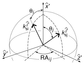
Figure 1: The angle differences. The declination is defined as ${\rm DEC}_{ij}:=\theta_{i}-\theta_{j}$. The lights enter from below in this figure.

These definitions are conceptually the same as in angles . We may set $\hat{x}^{\prime}{}$-axis and the other axes by the lights from some reference stars. For the derivation of Eq.(22), see Appendix B. We have constructed the angle differences by the scalars only, and hence they are invariant under coordinate transformations.

Next, we evaluate the angle differences (22) perturbatively. We focus on the case that the angle differences are much smaller than unity and the observer moves slowly, $v^{\hat{i}}\ll c$. Using a rotational transformation, we can set the spatial axes satisfied with

$$|k^{\hat{z}^{\prime}{}}_{s_{i}}|\gg|k^{\hat{x}^{\prime}{}}_{s_{i}}|,\ |k^{\hat{y}^{\prime}{}}_{s_{i}}|\ .$$ (23)

Since we consider the small angle differences, we can obtain the above inequality for all the right sources $\{s_{i}\}$ entering our small viewing angle. We restrict ourselves to the slowly boosted case so that we get the same inequality for the null momenta before the boost also:

$$|k^{\hat{z}}_{s_{i}}|\gg|k^{\hat{x}}_{s_{i}}|,\ |k^{\hat{y}}_{s_{i}}|\quad{\rm for}\ \forall s_{i}\ .$$ (24)

This implies $|k^{z}_{s_{i}}|\gg|k^{x}_{s_{i}}|,\ |k^{y}_{s_{i}}|$ in terms of the present coordinate system. We can always set the spatial coordinates satisfied with this inequality, without changing the form of the metric since the present coordinate system possesses rotational isometry. Then, we define the small parameters as

$$\alpha_{i}:=\frac{k^{\hat{x}}_{s_{i}}}{k^{\hat{z}}_{s_{i}}},\quad\beta_{i}:=\frac{k^{\hat{y}}_{s_{i}}}{k^{\hat{z}}_{s_{i}}}\ .$$ (25)

We use Eq.(25) and the observer’s velocity $v^{\hat{i}}$ as small parameters for the perturbative expansion. With the use of the null condition on a local Lorentz frame

$$|k^{\hat{0}}_{s_{i}}|=|k^{\hat{z}}_{s_{i}}|\sqrt{1+\alpha_{i}^{2}+\beta_{i}^{2}}\ ,$$ (26)

we can evaluate the small angle differences perturbatively as

$${\rm DEC}_{ij}$$

$$\simeq\frac{k_{s_{i}}^{\hat{x}^{\prime}}}{k_{s_{i}}^{\hat{z}^{\prime}}}-\frac{k_{s_{j}}^{\hat{x}^{\prime}{}}}{k_{s_{j}}^{\hat{z}^{\prime}{}}}+O\Big{(}\hat{v}\cdot(\alpha_{i}^{2},\beta_{i}^{2}),\ \hat{v}^{2}\cdot(\alpha_{i},\beta_{i})\Big{)}$$

$$=(\alpha_{i}-\alpha_{j})(1+v^{\hat{z}})$$

$$\quad+O\Big{(}\hat{v}\cdot(\alpha_{i}^{2},\beta_{i}^{2}),\ \hat{v}^{2}\cdot(\alpha_{i},\beta_{i})\Big{)},$$

$${\rm RA}_{ij}$$

$$\simeq\frac{k_{s_{i}}^{\hat{y}^{\prime}}}{k_{s_{i}}^{\hat{z}^{\prime}}}-\frac{k_{s_{j}}^{\hat{y}^{\prime}{}}}{k_{s_{j}}^{\hat{z}^{\prime}{}}}+O\Big{(}\hat{v}\cdot(\alpha_{i}^{2},\beta_{i}^{2}),\ \hat{v}^{2}\cdot(\alpha_{i},\beta_{i})\Big{)}$$

$$=(\beta_{i}-\beta_{j})(1+v^{\hat{z}})$$

$$\quad+O\Big{(}\hat{v}\cdot(\alpha_{i}^{2},\beta_{i}^{2}),\ \hat{v}^{2}\cdot(\alpha_{i},\beta_{i})\Big{)},$$ (27)

where we ignore the third and higher order terms of ($\alpha_{i},\,\beta_{i}$). Up to this order, the effect of boost corresponds to that of a simple Galilei transformation.

In the present coordinate system (II), due to the spatially conformal flatness, we can reduce Eq.(25) to

$$\alpha_{i}=\frac{v^{x}_{P}(t_{s_{i}};t_{o})}{v^{z}_{P}(t_{s_{i}};t_{o})},\quad\beta_{i}=\frac{v^{y}_{P}(t_{s_{i}};t_{o})}{v^{z}_{P}(t_{s_{i}};t_{o})}\ .$$ (28)

where $v_{P}^{i}(t_{s_{i}};t_{o})$ is given by Eq.(II). Expanding Eq.(28) around the leading solutions obtained for the flat spacetime, we get

$$\alpha_{i} =\alpha_{i}^{(0)}-\frac{1}{12}\Lambda r_{os_{i}}^{2}\frac{z_{s_{i}}x_{o}-x_{s_{i}}z_{o}}{(z_{o}-z_{s_{i}})^{2}}$$

$$-\sum_{J}\frac{2GM_{J}}{r_{oJ}}\left[\frac{(z_{o}-z_{J})(x_{s_{i}}-x_{J})}{r_{oJ}r_{s_{i}J}+\vec{r}_{oJ}\cdot\vec{r}_{s_{i}J}}\right.$$

$$\quad-\left.\frac{(x_{o}-x_{J})(z_{s_{i}}-z_{J})}{r_{oJ}r_{s_{i}J}+\vec{r}_{oJ}\cdot\vec{r}_{s_{i}J}}\right]$$

$$+O\left(\frac{GM_{J}}{r_{oJ}}\cdot({\alpha_{i}^{(0)}}^{2},{\beta_{i}^{(0)}}^{2})\right)$$ (29)

$$\beta_{i} =\beta_{i}^{(0)}-\frac{1}{12}\Lambda r_{os_{i}}^{2}\frac{z_{s_{i}}y_{o}-y_{s_{i}}z_{o}}{(z_{o}-z_{s_{i}})^{2}}$$

$$-\sum_{J}\frac{2GM_{J}}{r_{oJ}}\left[\frac{(z_{o}-z_{J})(y_{s_{i}}-y_{J})}{r_{oJ}r_{s_{i}J}+\vec{r}_{oJ}\cdot\vec{r}_{s_{i}J}}\right.$$

$$\quad-\left.\frac{(y_{o}-y_{J})(z_{s_{i}}-z_{J})}{r_{oJ}r_{s_{i}J}+\vec{r}_{oJ}\cdot\vec{r}_{s_{i}J}}\right]$$

$$+O\left(\frac{GM_{J}}{r_{oJ}}\cdot({\alpha_{i}^{(0)}}^{2},{\beta_{i}^{(0)}}^{2})\right)\ ,$$ (30)

where

$$\alpha_{i}^{(0)}:=\frac{x_{o}-x_{s_{i}}}{z_{o}-z_{s_{i}}},\quad\beta_{i}^{(0)}:=\frac{y_{o}-y_{s_{i}}}{z_{o}-z_{s_{i}}}$$ (31)

are small parameters for the case of flat spacetime as the same as Eq.(25). Substituting them to Eq.(III), we finally obtain a perturbative expansion of the small angle differences by means of the present coordinate with clarifying the magnitude of the approximation errors.

IV A Practical example

In this section, we evaluate the effect of the lensing objects on the small angle differences by using the results of the previous section for a practical example.

First, we identify where and who the observer is. We consider the observer standing at the spatial origin $\vec{r}_{o}=\vec{0}$, who watches the isotropic cosmic space except for the lensing objects. This observer corresponds to an observer who observes the homogeneous and isotropic cosmic space on the flat slicing of the de Sitter spacetime. In reality, we do not necessarily see the (local) isotropic cosmic space, so that the angle differences observed by us and the observer at $\vec{r}_{o}=\vec{0}$ may deviate each other. However, if we move very slowly, we can ignore its effect on the angle differences. Here, we evaluate the angle differences regarding ourselves as the rest observer at the spatial origin.

Next, we consider the lensing objects. We give the solar system and Sagittarius A*(Sgr A*), a supermassive black hole candidate at our galactic center, as the lensing objects, and consider stars or flares near around Sgr A*, like S-stars, as the light sources. In the sum of lensing objects, we denote the solar system objects by the index $I$ and Sgr A* by the index $B$: $\sum_{J}=\sum_{I,B}$. We set the $z$-axis as the null momenta from the light sources around Sgr A* are satisfied with $|k^{z}_{s_{i}}|\gg|k^{x}_{s_{i}}|,\ |k^{y}_{s_{i}}|$ and thus Eq.(24) also. This $z$-axis is almost the same as the line of sight to the light sources at a certain time. Also, we set the direction of $z$-axis as $z_{o}-z_{s_{i}}>0$. Since Sgr A* and the light sources are very far from the observer and the solar system, we approximately get

$$\frac{x_{o}-x_{B}}{z_{o}-z_{B}}\sim\alpha^{(0)}_{i},\ \frac{y_{o}-y_{B}}{z_{o}-z_{B}}\sim\beta^{(0)}_{i},\ \vec{r}_{s_{i}I}\sim\vec{r}_{s_{i}o},$$ (32)

which leads to

$$r_{oB} \simeq(z_{o}-z_{B})(1+O({\alpha_{i}^{(0)}}^{2},{\beta_{i}^{(0)}}^{2})),$$

$$r_{s_{i}I} \simeq(z_{I}-z_{s_{i}})(1+O({\alpha_{i}^{(0)}}^{2},{\beta_{i}^{(0)}}^{2})).$$ (33)

$(x_{B},y_{B},z_{B})$ denotes the spatial coordinates of Sgr A*. Using Eq.(32) and (IV), we can reduce Eq.(III) and (III) to

$$\alpha_{i} \simeq\alpha_{i}^{(0)}-\sum_{I}\frac{2GM_{I}}{r_{oI}}\frac{x_{o}-x_{I}}{r_{oI}+z_{I}-z_{o}}$$

$$-\frac{2GM_{B}}{r_{oB}}\frac{x_{s_{i}}-x_{B}}{r_{s_{i}B}+z_{s_{i}}-z_{B}}$$

$$+O\left(\frac{GM_{J}}{r_{oJ}}\cdot(\alpha_{i}^{(0)},\beta_{i}^{(0)})\right),$$ (34)

$$\beta_{i} \simeq\beta_{i}^{(0)}-\sum_{I}\frac{2GM_{I}}{r_{oI}}\frac{y_{o}-y_{I}}{r_{oI}+z_{I}-z_{o}}$$

$$-\frac{2GM_{B}}{r_{oB}}\frac{y_{s_{i}}-y_{B}}{r_{s_{i}B}+z_{s_{i}}-z_{B}}$$

$$+O\left(\frac{GM_{J}}{r_{oJ}}\cdot(\alpha_{i}^{(0)},\beta_{i}^{(0)})\right)\ .$$ (35)

The cosmological constant term vanishes for the rest observer at the spatial origin. For the sun, $GM_{\odot}/r_{o\odot}\sim 5$ miliarcsecond (mas), and for Sgr A*, $GM_{B}/r_{oB}\sim 10$ microarcsecond ($\mu$as) using estimated values for their masses and distances. The leading terms $\alpha_{i}^{(0)}$ and $\beta_{i}^{(0)}$ should be larger than these values not to break down the perturbative expansion. In the present approximation, the deflection of light by the solar system does not depend on the positions of each sources $\vec{r}_{s_{i}}$ while the deflection by Sgr A* does. When we derive the angle differences, therefore, the deflection by the solar system cancels out and only the deflection by Sgr A* remains:

$${\rm DEC}_{ij} =\alpha_{i}^{(0)}-\alpha_{j}^{(0)}$$

$$-\frac{2GM_{B}}{r_{oB}}\left(\frac{x_{s_{i}}-x_{B}}{r_{s_{i}B}+z_{s_{i}}-z_{B}}-\frac{x_{s_{j}}-x_{B}}{r_{s_{j}B}+z_{s_{j}}-z_{B}}\right)$$

$$+O\left(\frac{GM_{J}}{r_{oJ}}\cdot(\alpha_{i}^{(0)},\beta_{i}^{(0)})\right),$$

$${\rm RA}_{ij} =\beta_{i}^{(0)}-\beta_{j}^{(0)}$$

$$-\frac{2GM_{B}}{r_{oB}}\left(\frac{y_{s_{i}}-y_{B}}{r_{s_{i}B}+z_{s_{i}}-z_{B}}-\frac{y_{s_{j}}-y_{B}}{r_{s_{j}B}+z_{s_{j}}-z_{B}}\right)$$

$$+O\left(\frac{GM_{J}}{r_{oJ}}\cdot(\alpha_{i}^{(0)},\beta_{i}^{(0)})\right)\ .$$ (36)

We consider the rest observer, so we set $v^{\hat{i}}=0$. The deflection by the solar system exists certainly and can be the largest relativistic correction. We can regard it, however, as if it does not exist because of the canceling out in the angle differences.

In the case that a flare and S0-2, a star orbiting around Sgr A*, are the light sources, we obtain $\sim 100$ mas for the angle differences between them with $0.3$ mas errors by the latest observation Abuter:2020dou .

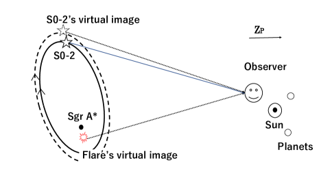
Figure 2: The schematic picture of S0-2, the (virtual image of) flare near Sgr A* and the solar system. The spatial distances between the objects are extremely scaled up or down. S0-2 orbits around Sgr A*(real oval line) and the light from S0-2 (real blue line) enters the observer. The incident lights from S0-2 and the flare show us the virtual images of them. The angle between the real image and the virtual image consists of $\sim 10$ $\mu$as by Sgr A* and $\sim 5$ mas by the solar system, respectively. We do not need to take into account the deflections by the solar system for the lights from S0-2 and the flare since the deflections cancel out between the two lights.

Using the result (IV), we find that the deflection by Sgr A* contributes about $10\ \mu$as to the angle differences, which would be detectable in the next-generation observational instrument. The approximation errors are suppressed around $0.1\ \mu$as at most. Thus, we now become able to verify the general relativistic effect to the light ray more precisely by comparing the near-future observational data to our formula derived here. We note that our expression (IV) can be easily applied for the model fitting to the actual observational data since they concretely consist of the spatial points of the light sources and the lensing objects parametrized by the coordinate time. For the observation of S0-2 and Sgr A*, the interval of proper time of us is almost the same as the interval of coordinate time, so that we can directly compare the theoretical expression (IV) parametrized by the coordinate time to the observational data. We evaluate the same angle differences in another coordinate system and confirm that the angle differences are invariant under the coordinate transformation at least up to the present order of approximation. See Appendix C.

Why does not the cosmological constant appear in the angle differences here? This is because the angle differences are constructed by the tetrad and the null momenta at the spatial origin only, where the effect of the cosmological constant vanishes from the metric tensor. Thus, though the lights travel a long distance, the rest observer at the spatial origin does not explicitly observe the effect of the cosmological constant. We note, however, that the cosmological constant affects the motions of the light sources. For the null momenta, the positions of the light sources are a part of their initial conditions, so that the cosmological constant is implicitly encoded into the angle differences through the positions of the light sources $\vec{r}_{s_{i}}$. If we monitor the motions of the light sources such as S0-2 continuously, we could find the effect of the cosmological constant from the time evolution of the positions of the light sources.

How will the situation change for a slowly moving observer around the spatial origin? If we regard the position of the observer is just a small variation from the spatial origin as $\vec{r}_{o}\simeq\vec{v}_{o}\delta t$ in the small-time interval $\delta t$ with the small velocity $\vec{v}_{o}$, the deviation of the angle differences remains around $\Lambda r_{s_{i}o}|\vec{v}_{o}|\delta t$. This variation can be ignorable in the observation if the cosmological constant and the velocity of the observer are sufficiently small in the small time interval.

V Summary

We have derived the spatially conformal flat metric perturbatively which describes the de Sitter spacetime with multi-lensing objects. We solved the null geodesic on that spacetime perturbatively around the uniform linear motion, parametrized by the coordinate time. Using the two world points, the points of the light source and the observer, we expressed the apparent velocities of the light at the light source and at the observer.

Then, we have defined the angle differences between two light rays entering the observer in the coordinate invariant way. The angle differences are constructed by the scalars defined in the observer’s local rest frame only so that they are coordinate invariant and hence can be observables. We reduced the coordinate invariant formula for the small angle differences case. For the small angle differences, due to the spatially conformal flatness of the present coordinate system, we can express them easily by means of the apparent velocities of the light at the observer.

Using the coordinate invariant formula, as a practical example, we evaluated the angle differences between the light rays from the star S0-2 and the flare around Sgr A*. We considered Sgr A* and the solar system as the lensing objects. The lights are deflected by both the solar system and Sgr A*. Up to the first order of the relativistic corrections, however, we find that the deflections by the solar system cancel out and only the deflections by Sgr A* remain in the small angle differences. We have shown that the deflections by Sgr A* can be about $10\ \mu$as, which would be detectable in the near-future observation. Also, we confirmed the coordinate invariance of the angle differences calculating them in another coordinate system.

On the other hand, we find that the cosmological constant does not appear in the angle differences explicitly for the rest observer who sees the isotropic cosmic space. We defined the angle differences by the null momenta and the tetrad at the observer only, and in the coordinate we use, the effect of the cosmological constant at the observer vanishes. For the case that the observer moves slowly, the effect on the angle differences is to be proportional to the cosmological constant and the velocity of the observer in the small time interval. If those quantities are sufficiently small, we can still ignore the effect of the cosmological constant for the angle differences. We emphasize, however, that the effect of the cosmological constant is implicitly taken into account in the motions of the light sources. Thus, if we can express the motions of the light sources with the cosmological constant, we may determine the effect of the cosmological constant comparing our formulae to the observational data of the angle differences. Monitoring the motions of the light sources such as S0-2 continuously, we expect to give some upper limit to the local cosmological constant.

Appendix A Static slice to isotropic slice at the first order of perturbation

We consider a coordinate transformation from the static coordinate of de Sitter spacetime denoted by $(t,\vec{r}_{S})$, to the isotropic coordinate denoted by $(t,\vec{r})$ up to the first order of perturbation. For simplicity, we ignore all the lensing objects. First, we rewrite the static coordinate of de Sitter spacetime as follows:

$$ds^{2} =-\left(1-\frac{1}{3}\Lambda r_{S}^{2}\right)dt^{2}+\frac{dr_{S}^{2}}{1-\frac{1}{3}\Lambda r_{S}^{2}}+r_{S}^{2}d\Omega_{2}$$

$$=-\left(1-\frac{1}{3}\Lambda r_{S}^{2}\right)dt^{2}+\frac{(dr_{S}/dr)^{2}}{1-\frac{1}{3}\Lambda r_{S}^{2}}dr^{2}$$

$$\quad+\frac{r_{S}^{2}}{r^{2}}\left(r^{2}d\Omega_{2}\right)\ ,$$ (37)

where $d\Omega_{2}$ is the infinitesimal 2-dimensional solid angle. Transforming to the isotropic one, we need a relation

$$\frac{dr}{r} =\frac{dr_{S}}{r_{S}\left(1-\frac{1}{3}\Lambda r_{S}^{2}\right)^{1/2}}$$

$$\simeq\left(\frac{1}{r_{S}}+\frac{1}{6}\Lambda r_{S}\right)dr_{S}\ .$$ (38)

In the second line, we expanded the denominator treating the $\Lambda$ term as a small quantity. Integrating the both sides, without the integration constant, we obtain

$$r \simeq r_{S}+\frac{1}{12}\Lambda r_{S}^{3},$$ (39)

$$ds^{2} =-\left(1-\frac{1}{3}\Lambda r^{2}\right)dt^{2}$$

$$\quad+\left(1-\frac{1}{6}\Lambda r^{2}\right)(dr^{2}+r^{2}d\Omega_{2})\ .$$ (40)

The isotropic coordinate is a good approximation around the spatial origin as long as the $\Lambda$ term is smaller than unity. If we want to include the lensing objects, we just need to add linear perturbations to the above metric and solve the perturbed Einstein equation as in Eq.(II).

Appendix B Derivation of the angle differences

We derive the angle differences (22). First, we derive the right ascension ${\rm RA}_{ij}$. An angle $\Theta_{ij}$ between two momenta $k_{s_{i}}^{\hat{i}^{\prime}{}}$ and $k_{s_{j}}^{\hat{i}^{\prime}{}}$ is given as

$$\Theta_{ij}={\rm arccos}\left(\frac{k_{s_{i}}^{\hat{i}^{\prime}{}}{k_{s_{j}}^{\hat{i}^{\prime}{}}}}{|k_{s_{i}}^{\hat{j}^{\prime}{}}||k_{s_{j}}^{\hat{k}^{\prime}{}}|}\right)$$ (41)

We define ${\rm RA}_{ij}$ as a projection of $\Theta_{ij}$ to $\hat{y}^{\prime}{}\hat{z}^{\prime}{}$-plane. That is achived by taking an angle between 2-dimensional momenta projected to $\hat{y}^{\prime}{}\hat{z}^{\prime}{}$-plane. Denoting ${\hat{l}^{a^{\prime}{}}}_{s_{i}}=(k_{s_{i}}^{\hat{y}^{\prime}{}},\,k_{s_{i}}^{\hat{z}^{\prime}{}})$, we obtain

$${\rm RA}_{ij} ={\rm arccos}\left(\frac{{\hat{l}^{a^{\prime}{}}}_{s_{i}}{\hat{l}^{a^{\prime}{}}}_{s_{j}}}{|{\hat{l}^{b^{\prime}{}}}_{s_{i}}||{\hat{l}^{c^{\prime}{}}}_{s_{j}}|}\right)$$

$$={\rm arccos}\left(\frac{k^{\hat{y}^{\prime}{}}_{s_{i}}k^{\hat{y}^{\prime}{}}_{s_{j}}+k^{\hat{z}^{\prime}{}}_{s_{i}}k^{\hat{z}^{\prime}{}}_{s_{j}}}{\hat{l}_{s_{i}}^{\prime}{}\hat{l}_{s_{j}}^{\prime}{}}\right)\ ,$$

$$\hat{l}_{s_{i}}^{\prime}{} =\sqrt{{k^{\hat{y}^{\prime}{}}_{s_{i}}}^{2}+{k^{\hat{z}^{\prime}{}}_{s_{i}}}^{2}}\ .$$ (42)

Next, we derive the declination ${\rm DEC}_{ij}$. We denote an angle between momentum $k_{s_{i}}^{\hat{i}^{\prime}{}}$ and $\hat{x}^{\prime}{}$-axis as $\theta_{i}$, which gives

$${\rm cos}\theta_{i}=\frac{k^{\hat{x}^{\prime}{}}_{s_{i}}}{|k^{\hat{i}^{\prime}{}}_{s_{i}}|},\quad{\rm sin}\theta_{i}=\frac{\hat{l}_{s_{i}}^{\prime}{}}{|k^{\hat{i}^{\prime}{}}_{s_{i}}|}\ .$$ (43)

We define ${\rm DEC}_{ij}$ as $\theta_{i}-\theta_{j}$ and thus we obtain

$${\rm DEC}_{ij} ={\rm arccos}({\rm cos}(\theta_{i}-\theta_{j}))$$

$$={\rm arccos}\left(\frac{k_{s_{i}}^{\hat{x}^{\prime}{}}k_{s_{j}}^{\hat{x}^{\prime}{}}+\hat{l}_{s_{i}}^{\prime}{}\hat{l}_{s_{j}}^{\prime}{}}{\sqrt{{k^{\hat{x}^{\prime}{}}_{s_{i}}}^{2}+\hat{l}_{s_{i}}^{\prime}{}^{2}}\sqrt{{k^{\hat{x}^{\prime}{}}_{s_{j}}}^{2}+\hat{l}_{s_{j}}^{\prime}{}^{2}}}\right)\ .$$ (44)

Appendix C Coordinate invariance of the angle differences

We consider a coordinate transformation by which Sgr A* becomes to stand at the spatial origin in the new coordinate system. We assume that the spatial part of the world line for Sgr A* in the coordinate (II) is given as

$$\vec{r}_{B}=\vec{r}_{B,{\rm ini}}+\vec{v}_{B}t,\quad|\vec{v}_{B}|\ll c,$$

$$\vec{r}_{B,{\rm ini}},\ \vec{v}_{B}:{\rm constants},$$ (45)

and transform it to $\vec{\tilde{r}}_{B}=\vec{0}$ in the new coordinate $(\tilde{t},\vec{\tilde{r}})$. We note that in the coordinate system (II), Sgr A* and the other lensing objects move slowly though we can ignore their velocities in the metric and the energy-momentum tensor as the first-order approximation. They move, however, against the rest observer considered in Sec.IV. By the coordinate transformation, the rest observer at the spatial origin in the coordinate (II) changes to a moving observer. The new coordinate corresponds to the galactic coordinate if $\Lambda=0$, and it is a convenient coordinate for various astrophysical models. We can change to the new coordinate by the following transformation:

$$\tilde{t} =\gamma_{B}[t-\vec{v}_{B}\cdot(\vec{r}-\vec{r}_{B,{\rm ini}})]\ ,$$

$$\vec{\tilde{r}} =\vec{r}-\vec{r}_{o}+\frac{(\gamma_{B}-1)}{v_{B}^{2}}\vec{v}_{B}\cdot(\vec{r}-\vec{r}_{B})\vec{v}_{B}\ ,$$

$$v_{B} :=|\vec{v}_{B}|,\quad\gamma_{B}:=1/\sqrt{1-v_{B}^{2}}\ .$$ (46)

This consists of a spatial translation and a boost in terms of the coordinate system. The rest observer at the spatial origin in the coordinate (II) transforms to

$$\vec{\tilde{r}}_{o} =-\tilde{\vec{r}}_{o,{\rm ini}}-\vec{v}_{B}\tilde{t},$$

$$\tilde{\vec{r}}_{o,{\rm ini}} :=\vec{r}_{B,{\rm ini}}+\left(\gamma_{B}-\frac{\gamma_{B}-1}{v_{B}^{2}}\right)(\vec{v}_{B}\cdot\vec{r}_{B,{\rm ini}})\vec{v}_{B}\ .$$ (47)

We obtain the following metric in the new coordinate system up to the first order of perturbation:

$$ds^{2} =-\left(1-\sum_{J}\frac{2GM_{J}}{|\vec{\tilde{r}}-\vec{\tilde{r}}_{J}|}-\frac{1}{3}\Lambda|\vec{\tilde{r}}-\vec{\tilde{r}}_{o}|^{2}\right)d\tilde{t}^{2}$$

$$\quad+\left(1+\sum_{J}\frac{2GM_{J}}{|\vec{\tilde{r}}-\vec{\tilde{r}}_{J}|}-\frac{1}{6}\Lambda|\vec{\tilde{r}}-\vec{\tilde{r}}_{o}|^{2}\right)d\vec{\tilde{r}}^{2}\ .$$ (48)

Even in the new coordinate system, the metric remains spatially conformal flat up to the first order of perturbation, and the effect of the cosmological constant vanishes at the moving observer.

Then, we calculate and compare the angle differences observed at $\vec{\tilde{r}}_{o}$ and $\vec{r}_{o}$ in the both coordinates. In the coordinate (C), the observer moves slowly with his/her velocity $-\vec{v}_{B}$ so that we need the Lorentz boost to the local rest frame to get observables. For the small angle differences, we obtain

$$\widetilde{\rm DEC}_{ij}\simeq\frac{\tilde{k}^{\hat{x}^{\prime}{}}_{s_{i}}}{\tilde{k}^{\hat{z}^{\prime}{}}_{s_{i}}}-\frac{\tilde{k}^{\hat{x}^{\prime}{}}_{s_{j}}}{\tilde{k}^{\hat{z}^{\prime}{}}_{s_{j}}},$$ (49)

$$\tilde{k}^{\hat{\alpha}^{\prime}{}}_{s_{i}}=\Lambda^{\hat{\alpha}}_{B\hat{\beta}}{\tilde{e}^{\hat{\beta}}_{\ \mu}\frac{\partial\tilde{x}^{\mu}}{\partial x^{\rho}}k^{\rho}_{s_{i}}},$$

$$\Lambda^{\hat{\alpha}}_{B\hat{\beta}}=\left(\begin{array}[]{cc}\hat{\gamma}_{B}&\hat{\gamma}_{B}v_{B}^{\hat{j}}\\ \hat{\gamma}_{B}v^{\hat{i}}_{B}&\delta_{\hat{i}\hat{j}}+(\hat{\gamma}_{B}-1)\frac{v^{\hat{i}}_{B}v^{\hat{j}}_{B}}{\hat{v}_{B}^{2}}\end{array}\right)\ ,$$ (52)

$$v_{B}^{\hat{i}}=\sqrt{|\tilde{g}^{00}|\tilde{g}_{ij}}v_{B}^{i},\quad\hat{\gamma}_{B}:=1/\sqrt{1-v_{B}^{\hat{i}}v_{B}^{\hat{i}}},$$

$${\tilde{e}^{\hat{0}}}_{\ \mu}=(1/\sqrt{|\tilde{g}^{00}|},\ 0,\ 0,\ 0),$$

$${\tilde{e}^{\hat{1}}}_{\ \mu}=(0,\ \sqrt{\tilde{g}_{11}},\ 0,\ 0),$$

$${\tilde{e}^{\hat{2}}}_{\ \mu}=(0,\ 0,\ \sqrt{\tilde{g}_{22}},\ 0),$$

$${\tilde{e}^{\hat{3}}}_{\ \mu}=(0,\ 0,\ 0,\ \sqrt{\tilde{g}_{33}}),$$

where all the quantities with the tilde are defined using the new coordinate (C), and $k^{\rho}_{s_{i}}$ is four-momentum of the light in the original coordinate (II). While, the small angle differences calculated in the original coordinate (II) is expressed as

$${\rm DEC}_{ij}\simeq\frac{k^{\hat{x}}_{s_{i}}}{k^{\hat{z}}_{s_{i}}}-\frac{k^{\hat{x}}_{s_{j}}}{k^{\hat{z}}_{s_{j}}},$$ (53)

$$k^{\hat{\alpha}}_{s_{i}}=e^{\hat{\alpha}}_{\ \rho}k^{\rho}_{s_{i}}\ .$$

Comparing Eq.(49) and (53), we can easily find that they correspond each other up to the first order of perturbation since we approximately hold the following relation

$$\Lambda^{\hat{\alpha}}_{B\hat{\beta}}\tilde{e}^{\hat{\beta}}_{\ \mu}\frac{\partial\tilde{x}^{\mu}}{\partial x^{\rho}}\simeq{e^{\hat{\alpha}}}_{\rho}\ .$$ (54)

We obtain the same result for $\widetilde{\rm RA}_{ij}$, and we can conclude that the angle differences defined in Eq.(III) are the coordinate invariant observables at least up to the first order of perturbation. We comment that by definition, the angle differences calculated in different coordinates will correspond each other even in a non-perturbative regime.

References

(1)
F. W. Dyson, A. S. Eddington and C. Davidson,
Phil. Trans. Roy. Soc. Lond. A 220, 291-333 (1920)
(2)
For example, see P. Schneider, J. Ehlers and E. E. Falco, “Gravitational Lenses”,
Springer, 1999.
(3)
G. W. Gibbons, C. M. Warnick and M. C. Werner,
Class. Quant. Grav. 25, 245009 (2008)
doi:10.1088/0264-9381/25/24/245009
[arXiv:0808.3074 [gr-qc]].
(4)
A. Ishihara, Y. Suzuki, T. Ono, T. Kitamura and H. Asada,
Phys. Rev. D 94, no.8, 084015 (2016)
doi:10.1103/PhysRevD.94.084015
[arXiv:1604.08308 [gr-qc]].
(5)
T. Ono and H. Asada,
Universe 5, no.11, 218 (2019)
doi:10.3390/universe5110218
[arXiv:1906.02414 [gr-qc]].
(6)
K. Takizawa, T. Ono and H. Asada,
Phys. Rev. D 101, no.10, 104032 (2020)
doi:10.1103/PhysRevD.101.104032
[arXiv:2001.03290 [gr-qc]].
(7)
F. de Felice, M. T. Crosta, A. Vecchiato, M. G. Lattanzi and B. Bucciarelli,
The Astrophysical Journal, vol 607, no.1 (2004).
(8)
R. Abuter et al. [GRAVITY],
Astron. Astrophys. 636, L5 (2020)
doi:10.1051/0004-6361/202037813
[arXiv:2004.07187 [astro-ph.GA]].