Bayesian Deep Learning via Subnetwork Inference

Abstract

The Bayesian paradigm has the potential to solve core issues of deep neural networks such as poor calibration and data inefficiency. Alas, scaling Bayesian inference to large weight spaces often requires restrictive approximations. In this work, we show that it suffices to perform inference over a small subset of model weights in order to obtain accurate predictive posteriors. The other weights are kept as point estimates. This subnetwork inference framework enables us to use expressive, otherwise intractable, posterior approximations over such subsets. In particular, we implement subnetwork linearized Laplace as a simple, scalable Bayesian deep learning method: We first obtain a MAP estimate of all weights and then infer a full-covariance Gaussian posterior over a subnetwork using the linearized Laplace approximation. We propose a subnetwork selection strategy that aims to maximally preserve the model’s predictive uncertainty. Empirically, our approach compares favorably to ensembles and less expressive posterior approximations over full networks. Our proposed subnetwork (linearized) Laplace method is implemented within the laplace PyTorch library (Daxberger et al., 2021) at https://github.com/AlexImmer/Laplace.

1 Introduction

A critical shortcoming of deep neural networks (NNs) is that they tend to be poorly calibrated and overconfident in their predictions, especially when there is a shift between the train and test data distributions (Nguyen et al., 2015; Guo et al., 2017). To reliably inform decision making, NNs need to robustly quantify the uncertainty in their predictions (Bhatt et al., 2020). This is especially important for safety-critical applications such as healthcare or autonomous driving (Amodei et al., 2016).

Bayesian modeling (Bishop, 2006; Ghahramani, 2015) presents a principled way to capture uncertainty via the posterior distribution over model parameters. Unfortunately, exact posterior inference is intractable in NNs. Despite recent successes in the field of Bayesian deep learning (Osawa et al., 2019; Maddox et al., 2019; Dusenberry et al., 2020), existing methods invoke unrealistic assumptions to scale to NNs with large numbers of weights. This severely limits the expressiveness of the inferred posterior and thus deteriorates the quality of the induced uncertainty estimates (Ovadia et al., 2019; Fort et al., 2019; Foong et al., 2019a).

Perhaps these unrealistic inference approximations can be avoided. Due to the heavy overparameterization of NNs, their accuracy is well-preserved by a small subnetwork (Cheng et al., 2017). Moreover, doing inference over a low-dimensional subspace of the weights can result in accurate uncertainty quantification (Izmailov et al., 2019). This prompts the following question: Can a full NN’s model uncertainty be well-preserved by a small subnetwork? In this work we demonstrate that the posterior predictive distribution of a full network can be well represented by that of a subnetwork. In particular, our contributions are as follows:

1. We propose subnetwork inference, a general framework for scalable Bayesian deep learning in which inference is performed over only a small subset of the NN weights, while all other weights are kept deterministic. This allows us to use expressive posterior approximations that are typically intractable in large NNs. We present a concrete instantiation of this framework that first fits a MAP estimate of the full NN, and then uses the linearized Laplace approximation to infer a full-covariance Gaussian posterior over a subnetwork (illustrated in Fig. 1).

2. We derive a subnetwork selection strategy based on the Wasserstein distance between the approximate posterior for the full network and the approximate posterior for the subnetwork. For scalability, we employ a diagonal approximation during subnetwork selection. Selecting a small subnetwork then allows us to infer weight covariances. Empirically, we find that making approximations during subnetwork selection is much less harmful to the posterior predictive than making them during inference.

3. We empirically evaluate our method on a range of benchmarks for uncertainty calibration and robustness to distribution shift. Our experiments demonstrate that expressive subnetwork inference can outperform popular Bayesian deep learning methods that do less expressive inference over the full NN as well as deep ensembles.

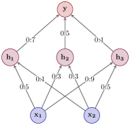
(a) Point Estimation

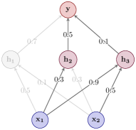
(b) Subnetwork Selection

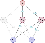
(c) Bayesian Inference

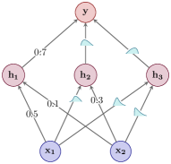
(d) Prediction

Figure 1: Schematic illustration of our proposed approach. (a) We train a neural network using standard techniques to obtain a point estimate of the weights. (b) We identify a small subset of the weights. (c) We estimate a posterior distribution over the selected subnetwork via Bayesian inference techniques. (d) We make predictions using the full network with a mix of Bayesian and deterministic weights.

2 Subnetwork Posterior Approximation

Let ${\mathbf{w}}\in\mathbb{R}^{D}$ be the $D$-dimensional vector of all neural network weights (i.e. the concatenation and flattening of all layers’ weight matrices). Bayesian neural networks (BNNs) aim to capture model uncertainty, i.e. uncertainty about the choice of weights ${\mathbf{w}}$ arising due to multiple plausible explanations of the training data $\mathcal{D}\!=\!\{{\mathbf{y}},{\mathbf{X}}\}$. Here, ${\mathbf{y}}\in\mathbb{R}^{O}$ is the output variable (e.g. classification label) and ${\mathbf{X}}\in\mathbb{R}^{N\times I}$ is the feature matrix. First, a prior distribution $p({\mathbf{w}})$ is specified over the BNN’s weights ${\mathbf{w}}$. We then wish to infer their full posterior distribution

$$p({\mathbf{w}}|\mathcal{D})\ =\ p({\mathbf{w}}|{\mathbf{y}},{\mathbf{X}})\ \propto\ p({\mathbf{y}}|{\mathbf{X}},{\mathbf{w}})p({\mathbf{w}})\ .$$ (1)

Finally, predictions for new data points ${\mathbf{X}}^{*}$ are made through marginalisation of the posterior:

$$p({\mathbf{y}}^{*}|{\mathbf{X}}^{*},\mathcal{D})=\int_{{\mathbf{w}}}p({\mathbf{y}}^{*}|{\mathbf{X}}^{*},{\mathbf{w}})p({\mathbf{w}}|\mathcal{D})d{\mathbf{w}}\ .$$ (2)

This posterior predictive distribution translates uncertainty in weights to uncertainty in predictions. Unfortunately, due to the non-linearity of NNs, it is intractable to infer the exact posterior distribution $p({\mathbf{w}}|\mathcal{D})$. It is even computationally challenging to faithfully approximate the posterior due to the high dimensionality of ${\mathbf{w}}$. Thus, crude posterior approximations such as complete factorization, i.e. $p({\mathbf{w}}|\mathcal{D})\approx\prod_{d=1}^{D}q({\textnormal{w}}_{d})$ where ${\textnormal{w}}_{d}$ is the $d^{\text{th}}$ weight in ${\mathbf{w}}$, are commonly employed (Hernández-Lobato & Adams, 2015; Blundell et al., 2015; Khan et al., 2018; Osawa et al., 2019). However, it has been shown that such an approximation suffers from severe pathologies (Foong et al., 2019a, b).

In this work, we question the widespread implicit assumption that an expressive posterior approximation must include all $D$ of the model weights. Instead, we try to perform inference only over a small subset of $S\ll D$ of the weights. The following arguments motivate this approach:

1. Overparameterization: Maddox et al. (2020) have shown that, in the neighborhood of local optima, there are many directions that leave the NN’s predictions unchanged. Moreover, NNs can be heavily pruned without sacrificing test-set accuracy (Frankle & Carbin, 2019). This suggests that the majority of a NN’s predictive power can be isolated to a small subnetwork.

2. Inference over submodels: Previous work has provided evidence that inference can be effective even when not performed on the full parameter space. Examples include Izmailov et al. (2019) and Snoek et al. (2015) who perform inference over low-dimensional projections of the weights, and only the last layer of a NN, respectively.

We therefore combine these two ideas and make the following two-step approximation of the posterior in Eq. 1:

$$p({\mathbf{w}}|\mathcal{D})\ \ \approx\ \ p({\mathbf{w}}_{S}|\mathcal{D})\ \prod_{r}\delta({\textnormal{w}}_{r}-\widehat{{\textnormal{w}}}_{r})$$ (3)

$$\approx\ \ q({\mathbf{w}}_{S})\ \prod_{r}\delta({\textnormal{w}}_{r}-\widehat{{\textnormal{w}}}_{r})\ \ =\ \ q_{S}({\mathbf{w}})\ .$$ (4)

The first approximation Eq. 3 decomposes the full NN posterior $p({\mathbf{w}}|\mathcal{D})$ into a posterior $p({\mathbf{w}}_{S}|\mathcal{D})$ over the subnetwork ${\mathbf{w}}_{S}\in\mathbb{R}^{S}$ and Dirac delta functions $\delta({\textnormal{w}}_{r}-\widehat{{\textnormal{w}}}_{r})$ over the $D-S$ remaining weights ${\textnormal{w}}_{r}$ to keep them at fixed values $\widehat{{\textnormal{w}}}_{r}\in\mathbb{R}$. Since posterior inference over the subnetwork is still intractable, Eq. 4 further approximates $p({\mathbf{w}}_{S}|\mathcal{D})$ by $q({\mathbf{w}}_{S})$. However, importantly, if the subnetwork is much smaller than the full network, we can afford to make $q({\mathbf{w}}_{S})$ more expressive than would otherwise be possible. We hypothesize that being able to capture rich dependencies across the weights within the subnetwork will provide better results than crude approximations applied to the full set of weights.

Relationship to Weight Pruning Methods. Note that the posterior approximation in Eq. 4 can be viewed as pruning the variances of the weights $\{{\textnormal{w}}_{r}\}_{r}$ to zero. This is in contrast to weight pruning methods (Cheng et al., 2017) that set the weights themselves to zero. I.e., weight pruning methods can be viewed as removing weights to preserve the predictive mean (i.e. to retain accuracy close to the full model). In contrast, subnetwork inference can be viewed as removing just the variances of certain weights—while keeping their means—to preserve the predictive uncertainty (e.g. to retain calibration close to the full model). Thus, they are complementary approaches. Importantly, by not pruning weights, subnetwork inference retains the full predictive power of the full NN to retain its predictive accuracy.

3 Background: Linearized Laplace

In this work we satisfy Eq. 4 by approximating the posterior distribution over the weights with the linearized Laplace approximation (MacKay, 1992). This is an inference technique that has recently been shown to perform strongly (Foong et al., 2019b; Immer et al., 2021b) and can be applied post-hoc to pre-trained models. We now describe it in a general setting. See Daxberger et al. (2021) for a more detailed description, review of recent advances, and software library for the Laplace approximation in deep learning.

We denote our NN function as ${\bm{f}}:\mathbb{R}^{I}\to\mathbb{R}^{O}$. We begin by defining a prior over our NN’s weights, which we choose to be a fully factorised Gaussian $p({\mathbf{w}})=\mathcal{N}({\mathbf{w}};\textbf{0},\lambda{\mathbf{I}})$. We find a local optimum of the posterior, also known as a maximum a posteriori (MAP) setting of the weights:

$$\widehat{{\mathbf{w}}}=\operatorname{arg\,max}_{{\mathbf{w}}}\left[\log p({\mathbf{y}}|{\mathbf{X}},{\mathbf{w}})+\log p({\mathbf{w}})\right].$$ (5)

The posterior is then approximated with a second order Taylor expansion around the MAP estimate:

$$\log p({\mathbf{w}}|\mathcal{D})\approx\log p(\widehat{{\mathbf{w}}}|\mathcal{D})\!-\!\frac{1}{2}({\mathbf{w}}-\widehat{{\mathbf{w}}})^{\top}{\mathbf{H}}({\mathbf{w}}-\widehat{{\mathbf{w}}})$$ (6)

where ${\mathbf{H}}\!\in\!\mathbb{R}^{D{\times}D}$ is the Hessian of the negative log-posterior density w.r.t. the network weights ${\mathbf{w}}$:

$${\mathbf{H}}=N\cdot\mathbb{E}_{p(\mathcal{D})}\left[-\partial^{2}\log p({\mathbf{y}}|{\mathbf{X}},{\mathbf{w}})/\partial{\mathbf{w}}^{2}\right]+\lambda{\mathbf{I}}\,.$$ (7)

Thus, the approximate posterior takes the form of a full-covariance Gaussian with covariance matrix ${\mathbf{H}}^{-1}$:

$$p({\mathbf{w}}|\mathcal{D})\approx q({\mathbf{w}})=\mathcal{N}\left({\mathbf{w}};\widehat{{\mathbf{w}}},{\mathbf{H}}^{-1}\right).$$ (8)

In practise, the Hessian ${\mathbf{H}}$ is commonly replaced with the generalized Gauss-Newton matrix (GGN) $\widetilde{{\mathbf{H}}}\in\mathbb{R}^{D\times D}$ (Martens & Sutskever, 2011; Martens, 2020, 2016)

$$\widetilde{{\mathbf{H}}}=\textstyle\sum_{n=1}^{N}{\mathbf{J}}_{n}^{\top}{\mathbf{H}}_{n}{\mathbf{J}}_{n}+\lambda{\mathbf{I}}\ .$$ (9)

Here, ${\mathbf{J}}_{n}=\partial{\bm{f}}({\mathbf{x}}_{n},{\mathbf{w}})/\partial{\mathbf{w}}\!\!\in\!\!\mathbb{R}^{O\times D}$ is the Jacobian of the model outputs ${\bm{f}}({\mathbf{x}}_{n},{\mathbf{w}})\!\!\in\!\!\mathbb{R}^{O}$ w.r.t. ${\mathbf{w}}$. ${\mathbf{H}}_{n}=-\partial^{2}\log p({\mathbf{y}}|{\bm{f}}({\mathbf{x}}_{n},{\mathbf{w}}))/\partial^{2}{\bm{f}}({\mathbf{x}}_{n},{\mathbf{w}})\in\mathbb{R}^{O\times O}$ is the Hessian of the negative log-likelihood w.r.t. model outputs.

Interestingly, when using a Gaussian likelihood, the Gaussian with a GGN precision matrix corresponds to the true posterior distribution when the NN is approximated with a first-order Taylor expansion around $\widehat{{\mathbf{w}}}$ (Khan et al., 2019; Immer et al., 2021b). The locally linearized function is

$${\bm{f}}_{\text{lin}}({\mathbf{x}},{\mathbf{w}})={\bm{f}}({\mathbf{x}},\widehat{{\mathbf{w}}})+\widehat{{\mathbf{J}}}({\mathbf{x}})({\mathbf{w}}-\widehat{{\mathbf{w}}})$$ (10)

where $\widehat{{\mathbf{J}}}({\mathbf{x}})=\partial{\bm{f}}({\mathbf{x}},\widehat{{\mathbf{w}}})/\partial\widehat{{\mathbf{w}}}\in\mathbb{R}^{O\times D}$. This turns the underlying probabilistic model from a BNN into a generalized linear model (GLM), where the Jacobian $\widehat{{\mathbf{J}}}({\mathbf{x}})$ acts as a basis function expansion. Making predictions with the GLM ${\bm{f}}_{\text{lin}}$ has been found to outperform the corresponding BNN ${\bm{f}}$ with the GGN-Laplace posterior (Lawrence, 2001; Foong et al., 2019b; Immer et al., 2021b). Additionally, the equivalence between a GLM and a linearized BNN will help us to derive a subnetwork selection strategy in Section 5.

The resulting posterior predictive distribution is

$$p({\mathbf{y}}^{*}|{\mathbf{x}}^{*},\mathcal{D})=\!\int\!p({\mathbf{y}}^{*}|{\bm{f}}_{\text{lin}}({\mathbf{x}}^{*},{\mathbf{w}}))p({\mathbf{w}}|\mathcal{D})\,d{\mathbf{w}}\ .$$ (11)

For regression, when using a Gaussian noise model $p({\mathbf{y}}^{*}|{\bm{f}}_{\text{lin}}({\mathbf{x}}^{*},{\mathbf{w}}))\!=\mathcal{N}({\mathbf{y}}^{*};{\bm{f}}_{\text{lin}}({\mathbf{x}}^{*},{\mathbf{w}}),\sigma^{2})$, our approximate distribution becomes exact $q({\mathbf{w}})=p({\mathbf{w}}|\mathcal{D})=\mathcal{N}({\mathbf{w}};\widehat{{\mathbf{w}}},\widetilde{{\mathbf{H}}}^{-1})$. We obtain the closed form predictive

$$p({\mathbf{y}}^{*}|{\mathbf{x}}^{*},\mathcal{D})=\mathcal{N}({\mathbf{y}}^{*};{\bm{f}}({\mathbf{x}}^{*},\widehat{{\mathbf{w}}}),\Sigma({\mathbf{x}}^{*}){+}\sigma^{2}{\mathbf{I}})\ ,$$ (12)

where $\Sigma({\mathbf{x}}^{*})\!=\!\widehat{{\mathbf{J}}}({\mathbf{x}}^{*})^{\top}\widetilde{{\mathbf{H}}}^{-1}\widehat{{\mathbf{J}}}({\mathbf{x}}^{*})$. For classification with a categorical likelihood $p({\mathbf{y}}^{*}|{\bm{f}}_{\text{lin}}({\mathbf{x}}^{*},{\mathbf{w}}))=\text{Cat}({\mathbf{y}}^{*};\phi({\bm{f}}_{\text{lin}}({\mathbf{x}}^{*},{\mathbf{w}}))$, the posterior is strictly convex. This makes our Gaussian a faithful approximation. Here, $\phi(\cdot)$ refers to the softmax function. The predictive integral has no analytical solution. Instead we leverage the probit approximation (Gibbs, 1998; Bishop, 2006):

$$p({\mathbf{y}}^{*}|{\mathbf{x}}^{*},\mathcal{D})\!\approx\!\text{Cat}\!\left(\!{\mathbf{y}}^{*};\phi\!\left(\frac{{\bm{f}}({\mathbf{x}}^{*},\widehat{{\mathbf{w}}})}{\sqrt{1{+}\frac{\pi}{8}\text{diag}(\Sigma({\mathbf{x}}^{*}))}}\right)\!\right).$$ (13)

These closed-form expressions are attractive since they result in the predictive mean and classification boundaries being exactly equal to those of the MAP estimated NN.

Unfortunately, storing the full $D\times D$ covariance matrix over the weight space of a modern NN (i.e. with very large $D$) is computationally intractable. There have been efforts to develop cheaper approximations to this object, such as only storing diagonal (Denker & LeCun, 1990) or block diagonal (Ritter et al., 2018; Immer et al., 2021b) entries, but these come at the cost of reduced predictive performance.

4 Linearized Laplace Subnetwork Inference

We outline the following procedure for scaling the linearized Laplace approximation to large neural network models within the framework of subnetwork inference.

Step #1: Point Estimation, Fig. 1 (a).

Train a neural network to obtain a point estimate of the weights, denoted $\widehat{{\mathbf{w}}}$. This can be done using stochastic gradient-based optimization methods (Goodfellow et al., 2016). Alternatively, we could make use of a pre-trained model.

Step #2: Subnetwork Selection, Fig. 1 (b).

Identify a small subnetwork ${\mathbf{w}}_{S}\in\mathbb{R}^{S},S\ll D$. Ideally, we would like to find the subnetwork which produces a predictive posterior ‘closest’ to the full-network’s predictive distribution. Regrettably, reasoning in the space of functions directly is challenging (Burt et al., 2020). Instead, in Section 5, we describe a strategy that minimizes the Wasserstein distance between the sub- and full-network’s weight posteriors.

Step #3: Bayesian Inference, Fig. 1 (c).

Use the GGN-Laplace approximation to infer a full-covariance Gaussian posterior over the subnetwork’s weights ${\mathbf{w}}_{S}\in\mathbb{R}^{S}$:

$$p({\mathbf{w}}_{S}|\mathcal{D})\approx q({\mathbf{w}}_{S})=\mathcal{N}({\mathbf{w}}_{S};\widehat{{\mathbf{w}}}_{S},\widetilde{{\mathbf{H}}}_{S}^{-1})$$ (14)

where $\widetilde{{\mathbf{H}}}_{S}\in\mathbb{R}^{S{\times}S}$ is the GGN w.r.t. the weights ${\mathbf{w}}_{S}$:

$$\widetilde{{\mathbf{H}}}_{S}=\textstyle\sum_{n=1}^{N}{\mathbf{J}}_{Sn}^{\top}{\mathbf{H}}_{n}{\mathbf{J}}_{Sn}+\lambda_{S}{\mathbf{I}}\ .$$ (15)

Here, ${\mathbf{J}}_{Sn}=\partial{\bm{f}}({\mathbf{x}}_{n},{\mathbf{w}}_{S})/\partial{\mathbf{w}}_{S}\!\!\in\!\!\mathbb{R}^{O\times S}$ is the Jacobian w.r.t. ${\mathbf{w}}_{S}$. ${\mathbf{H}}_{n}$ is defined as in Section 2. In order to best preserve the magnitude of the predictive variance, we update our prior precision to be $\lambda_{S}=\lambda\!\cdot\!\nicefrac{{S}}{{D}}$ (see Appendix C for more details). All weights not belonging to the chosen subnetwork are fixed at their MAP values. Note that this whole procedure (i.e. Steps #1-#3) is a perfectly valid mixed inference strategy: We perform full Laplace inference over the selected subnetwork and MAP inference over all remaining weights. The resulting approximate posterior Eq. 4 is

$$q_{S}({\mathbf{w}})\overset{(\ref{eq:subnetwork_laplace_posterior})}{=}\mathcal{N}({\mathbf{w}}_{S};\widehat{{\mathbf{w}}}_{S},\widetilde{{\mathbf{H}}}_{S}^{-1})\textstyle\prod_{r}\delta({\textnormal{w}}_{r}-\widehat{{\textnormal{w}}}_{r})\ .$$ (16)

Given a sufficiently small subnetwork ${\mathbf{w}}_{S}$, it is feasible to store and invert $\widetilde{{\mathbf{H}}}_{S}$. In particular, naively storing and inverting the full GGN $\widetilde{{\mathbf{H}}}$ scales as $\mathcal{O}(D^{2})$ and $\mathcal{O}(D^{3})$, respectively. Using the subnetwork GGN $\widetilde{{\mathbf{H}}}_{S}$ instead reduces this burden to $\mathcal{O}(S^{2})$ and $\mathcal{O}(S^{3})$, respectively. In our experiments, $S\,{\ll}\,D$ with our subnetworks representing less that 1% of the total weights. Note that quadratic/cubic scaling in $S$ is unavoidable if we are to capture weight correlations.

Step #4: Prediction, Fig. 1 (d).

Perform a local linearization of the NN (see Section 3) while fixing ${\mathbf{w}}_{r}$ to $\widehat{{\mathbf{w}}}_{r}$:

$${\bm{f}}_{\text{lin}}({\mathbf{x}},{\mathbf{w}}_{S})={\bm{f}}({\mathbf{x}},\widehat{{\mathbf{w}}})+\widehat{{\mathbf{J}}}_{S}({\mathbf{x}})({\mathbf{w}}_{S}-\widehat{{\mathbf{w}}}_{S})\ ,$$ (17)

where $\widehat{{\mathbf{J}}}_{S}({\mathbf{x}})=\partial{\bm{f}}({\mathbf{x}},\widehat{{\mathbf{w}}}_{S})/\partial\widehat{{\mathbf{w}}}_{S}\!\in\!\mathbb{R}^{O\times S}$. Following Eq. 12 and Eq. 13, the corresponding predictive distributions are

$$p({\mathbf{y}}^{*}|{\mathbf{x}}^{*},\mathcal{D})=\mathcal{N}({\mathbf{y}}^{*};{\bm{f}}({\mathbf{x}}^{*},\widehat{{\mathbf{w}}}),{\color[rgb]{1,0,0.5}\Sigma_{S}({\mathbf{x}}^{*})}{+}\sigma^{2}{\mathbf{I}})$$ (18)

for regression and

$$p({\mathbf{y}}^{*}|{\mathbf{x}}^{*},\mathcal{D})\approx\text{softmax}\left(\frac{{\bm{f}}({\mathbf{x}}^{*},\widehat{{\mathbf{w}}})}{\sqrt{1{+}\frac{\pi}{8}\text{diag}({\color[rgb]{1,0,0.5}\Sigma_{S}({\mathbf{x}}^{*})})}}\right)$$ (19)

for classification, where $\Sigma({\mathbf{x}}^{*})$ in Eq. 12 and Eq. 13 is substituted with ${\color[rgb]{1,0,0.5}\Sigma_{S}({\mathbf{x}}^{*})}=\widehat{{\mathbf{J}}}_{S}({\mathbf{x}}^{*})^{T}\widetilde{{\mathbf{H}}}_{S}^{-1}\widehat{{\mathbf{J}}}_{S}({\mathbf{x}}^{*})$.

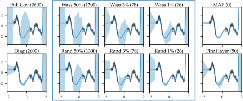
Figure 2: Predictive distributions (mean $\pm$ std) for 1D regression. The numbers in parentheses denote the number of parameters over which inference was done (out of 2600 in total). The blue box highlights subnetwork inference using Wasserstein (top) and random (bottom) subnetwork selection. Wasserstein subnetwork inference maintains richer predictive uncertainties at smaller parameter counts.

5 Subnetwork Selection

Ideally, we would like to choose a subnetwork such that the induced predictive posterior distribution is as close as possible to the predictive posterior provided by inference over the full network Eq. 11. This discrepancy between stochastic processes is often quantified through the functional Kullback-Leibler (KL) divergence (Sun et al., 2019; Burt et al., 2020):

$$\sup_{n\in{\mathbb{N}},{\mathbf{X}}^{*}\in\mathcal{X}^{n}}\!\!\!D_{\text{KL}}(p_{S}({\mathbf{y}}^{*}|{\mathbf{X}}^{*},\mathcal{D})\,||\,p({\mathbf{y}}^{*}|{\mathbf{X}}^{*},\mathcal{D})),$$ (20)

where $p_{S}$ denotes the subnetwork predictive posterior and $\mathcal{X}^{n}$ denotes a finite measurement set of $n$ elements. Regrettably, reasoning directly in function space is a difficult task (Nalisnick & Smyth, 2018; Pearce et al., 2019; Sun et al., 2019; Antorán et al., 2020; Nalisnick et al., 2021; Burt et al., 2020). Instead we focus our attention on weight space.

In weight space, our aim is to minimise the discrepancy between the exact posterior over the full network Eq. 1 and the subnetwork approximate posterior Eq. 4. This provides two challenges. Firstly, computing the exact posterior distribution remains intractable. Secondly, common discrepancies, like the KL divergence or the Hellinger distance, are not well defined for the Dirac delta distributions found in Eq. 4.

To solve the first issue, we again resort to local linearization, introduced in Section 3. The true posterior for the linearized model is Gaussian or approximately Gaussian:

$$p({\mathbf{w}}|\mathcal{D})\simeq\mathcal{N}({\mathbf{w}};\widehat{{\mathbf{w}}},\widetilde{{\mathbf{H}}}^{-1})\ .$$ (21)

We solve the second issue by choosing the squared 2-Wasserstein distance, which is well defined for distributions with disjoint support. For the case of a full covariance Gaussian Eq. 21 and a product of a full covariance Gaussian with Dirac deltas Eq. 16, this metric takes the following form:

$$W_{2}(p({\mathbf{w}}|\mathcal{D}),q_{S}({\mathbf{w}}))^{2}$$ (22)

$$=\text{Tr}\left(\widetilde{{\mathbf{H}}}^{-1}+\widetilde{{\mathbf{H}}}_{S+}^{-1}-2\left(\widetilde{{\mathbf{H}}}_{S+}^{-1/2}\widetilde{{\mathbf{H}}}^{-1}\widetilde{{\mathbf{H}}}_{S+}^{-1/2}\right)^{1/2}\right)\ ,$$

where the covariance matrix $\widetilde{{\mathbf{H}}}_{S+}^{-1}$ is equal to $\widetilde{{\mathbf{H}}}_{S}^{-1}$ padded with zeros at the positions corresponding to ${\textnormal{w}}_{r}$, matching the shape of $\widetilde{{\mathbf{H}}}^{-1}$. See Appendix B for details.

Finding the subset ${\mathbf{w}}_{S}\in\mathbb{R}^{S}$ of size $S$ that minimizes Eq. 22 would be combinatorially difficult, as the contribution of each weight depends on every other weight. To address this issue, we make an independence assumption among weights, resulting in the simplified objective

$$W_{2}(p({\mathbf{w}}|\mathcal{D}),q_{S}({\mathbf{w}}))^{2}\approx\sum_{d=1}^{D}\sigma^{2}_{d}(1-m_{d})\ ,$$ (23)

where $\sigma^{2}_{d}$ is the marginal variance of the $d^{\text{th}}$ weight, and $m_{d}=1$ if ${\textnormal{w}}_{d}\,\in\,{\mathbf{w}}_{S}$ and 0 otherwise (see Appendix B). The objective Eq. 23 is trivially minimized by a subnetwork containing the $S$ weights with highest variances. This is related to common magnitude-based weight pruning methods (Cheng et al., 2017). The main difference is that our selection strategy involves weight variances rather than magnitudes as we target predictive uncertainty rather than accuracy.

In practice, even computing the marginal variances (i.e. the diagonal of $\widetilde{{\mathbf{H}}}^{-1}$) is intractable, as it requires storing and inverting the GGN $\widetilde{{\mathbf{H}}}$. However, we can approximate posterior marginal variances with the diagonal Laplace approximation $\text{diag}(\widetilde{{\mathbf{H}}}^{-1})\!\approx\!\text{diag}(\widetilde{{\mathbf{H}}})^{-1}$ (Denker & LeCun, 1990; Kirkpatrick et al., 2017), diagonal SWAG (Maddox et al., 2019), or even mean-field variational inference (Blundell et al., 2015; Osawa et al., 2019). In this work we rely on the former two, as the the latter involves larger overhead.

It may seem that we have resorted to the poorly performing diagonal assumptions that we sought to avoid in the first place (Ovadia et al., 2019; Foong et al., 2019a; Ashukha et al., 2020). However, there is a key difference. We make the diagonal assumption during subnetwork selection rather than inference; we do full covariance inference over ${\mathbf{w}}_{S}$. In Section 6, we provide evidence that making a diagonal assumption during subnetwork selection is reasonable by showing that 1) it is substantially less harmful to predictive performance than making the same assumption during inference, and 2) it outperforms random subnetwork selection.

6 Experiments

We empirically assess the effectiveness of subnetwork inference compared to methods that do less expressive inference over the full network as well as state-of-the-art methods for uncertainty quantification in deep learning. We consider three benchmark settings: 1) small-scale toy regression, 2) medium-scale tabular regression, and 3) image classification with ResNet-18. Further experimental results and setup details are presented in Appendix A and Appendix D, respectively.

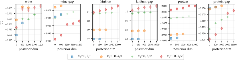
Figure 3: Mean test log-likelihood values obtained on UCI datasets across all splits. Different markers indicate models with different numbers of weights. The horizontal axis indicates the number of weights over which full covariance inference is performed. 0 corresponds to MAP parameter estimation, and the rightmost setting for each marker corresponds to full network inference.

6.1 How does Subnetwork Inference preserve Posterior Predictive Uncertainty?

We first assess how the predictive distribution of a full-covariance Gaussian posterior over a selected subnetwork qualitatively compares to that obtained from 1) a full-covariance Gaussian over the full network (Full Cov), 2) a factorised Gaussian posterior over the full network (Diag), 3) a full-covariance Gaussian over only the (Final layer) of the network (Snoek et al., 2015), and 4) a point estimate (MAP). For subnetwork inference, we consider both Wasserstein (Wass) (as described in Section 5) and uniform random subnetwork selection (Rand) to obtain subnetworks that comprise of only 50%, 3% and 1% of the model parameters. For this toy example, it is tractable to compute exact posterior marginal variances to guide subnetwork selection.

Our NN consists of 2 ReLU hidden layers with 50 hidden units each. We employ a homoscedastic Gaussian likelihood function where the noise variance is optimised with maximum likelihood. We use GGN-Laplace inference over network weights (not biases) in combination with the linearized predictive distribution in Eq. 18. Thus, all approaches considered share their predictive mean, allowing better comparison of their uncertainty estimates. We set the full network prior precision to $\lambda=3$ (a value which we find to work well empirically) and set $\lambda_{S}=\lambda\cdot\nicefrac{{S}}{{D}}$.

We use a synthetic 1D regression task with two separated clusters of inputs (Antorán et al., 2020), allowing us to probe for ‘in-between’ uncertainty (Foong et al., 2019b). Results are shown in Fig. 2. Subnetwork inference preserves more of the uncertainty of full network inference than diagonal Gaussian or final layer inference while doing inference over fewer weights. By capturing weight correlations, subnetwork inference retains uncertainty in between clusters of data. This is true for both random and Wasserstein subnetwork selection. However, the latter preserves more uncertainty with smaller subnetworks. Finally, the strong superiority to diagonal Laplace shows that making a diagonal assumption for subnetwork selection but then using a full-covariance Gaussian for inference (as we do) performs significantly better than making a diagonal assumption for the inferred posterior directly (cf. Section 5). These results suggest that expressive inference over a carefully selected subnetwork retains more predictive uncertainty than crude approximations over the full network.

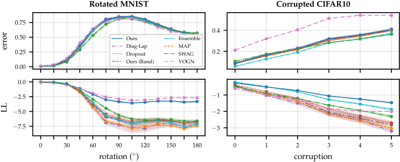
Figure 4: Results on the rotated MNIST (left) and the corrupted CIFAR (right) benchmarks, showing the mean $\pm$ std of the error (top) and log-likelihood (bottom) across three different seeds. Subnetwork inference retains better uncertainty calibration and robustness to distribution shift than point-estimated networks and other Bayesian deep learning approaches. See Appendix A for ECE and Brier score results.

6.2 Subnetwork Inference in Large Models vs Full Inference over Small Models

Secondly, we study how subnetwork inference in larger NNs compares to full network inference in smaller ones. We explore this by considering 4 fully connected NNs of increasing size. These have numbers of hidden layers $h_{d}{=}\{1,2\}$ and hidden layer widths $w_{d}{=}\{50,100\}$. For a dataset with input dimension $i_{d}$, the number of weights is given by $D{=}(i_{d}{+}1)w_{d}{+}(h_{d}{-}1)w_{d}^{2}$. Our 2 hidden layer, 100 hidden unit NNs have a weight count of the order $10^{4}$. Full covariance inference in these NNs borders the limit of computational tractability on commercial hardware. We first obtain a MAP estimate of each NN’s weights and our homoscedastic likelihood function’s noise variance. We then perform full network GGN-Laplace inference for each NN. We also use our proposed Wassertein rule to prune every NN’s weight variances such that the number of variances that remain matches the size of every smaller NN under consideration. We employ the diagonal Laplace approximation to cheaply estimate posterior marginal variances for subnetwork selection. We employ the linearization in Eq. 12 and Eq. 18 to compute predictive distributions. Consequently, NNs with the same number of weights make the same mean predictions. Increasing the number of weight variances considered will thus only increase predictive uncertainty.

We employ 3 tabular datasets of increasing size (input dimensionality, n. points): wine (11, 1439), kin8nm (8, 7373) and protein (9, 41157). We consider their standard train-test splits (Hernández-Lobato & Adams, 2015) and their gap variants (Foong et al., 2019b), designed to test for out-of-distribution uncertainty. Details are provided in Section D.4. For each split, we set aside 15% of the train data as a validation set. We use these for early stopping when finding MAP estimates and for selecting the weights’ prior precision. We keep other hyperparameters fixed across all models and datasets. Results are shown in Fig. 3.

We present mean test log-likelihood (LL) values, as these take into account both accuracy and uncertainty. Larger ($w_{d}=100,h_{d}=2$) models tend to perform best when combined with full network inference, although Wine-gap and Protein-gap are exceptions. Interestingly, these larger models are still best when we perform inference over subnetworks of the size of smaller models. We conjecture this is due to an abundance of degenerate directions (i.e. weights) in the weight posterior NN models (Maddox et al., 2020). Full network inference in small models captures information about both useful and non-useful weights. In larger models, our subnetwork selection strategy allows us to dedicate a larger proportion of our resources to modelling informative weight variances and covariances. In 3 out of 6 datasets, we find abrupt increases in LL as we increase the number of weights over which we perform inference, followed by a plateau. Such plateaus might be explained by most of the informative weight variances having already been accounted for. Considering that the cost of computing the GGN dominates that of NN training, these results suggest that, given the same amount of compute, it is better to perform subnetwork inference in larger models than full network inference in small ones.

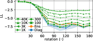
(a) Rotated MNIST

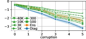
(b) Corrupted CIFAR10

Subnet Size	Memory
11.2M (100%)	500TB
40K (0.36%)	6.4GB
1K (0.01%)	4.0MB
100 (0.001%)	40KB

(c) Memory Footprints

Figure 5: Log-likelihoods of our method with subnetwork sizes between 100-40K using ResNet-18 on rotated MNIST (left) and corrupted CIFAR10 (middle), vs. Ensembles and Diagonal Laplace, and respective covariance matrix memory footprints (right). For all subnetwork sizes, we use the same hyperparameters as in Section 6.3 (i.e. no individual tuning per size). Performance degrades smoothly with subnetwork size, but our method retains strong calibration even with very small subnetworks (requiring only marginal extra memory).

6.3 Image Classification under Distribution Shift

We now assess the robustness of large convolutional neural networks with subnetwork inference to distribution shift on image classification tasks compared to the following baselines: point-estimated networks (MAP), Bayesian deep learning methods that do less expressive inference over the full network: MC Dropout (Gal & Ghahramani, 2016), diagonal Laplace, VOGN (Osawa et al., 2019) (all of which assume factorisation of the weight posterior), and SWAG (Maddox et al., 2019) (which assumes a diagonal plus low-rank posterior). We also benchmark deep ensembles (Lakshminarayanan et al., 2017). The latter is considered state-of-the-art for uncertainty quantification in deep learning (Ovadia et al., 2019; Ashukha et al., 2020). We use ensembles of 5 NNs, as suggested by (Ovadia et al., 2019), and 16 samples for MC Dropout, diagonal Laplace and SWAG. We use a Dropout probability of $0.1$ and a prior precision of $\lambda=4\times 10^{4}$ for diagonal Laplace, found via grid search. We apply all approaches to ResNet-18 (He et al., 2016), which is composed of an input convolutional block, 8 residual blocks and a linear layer, for a total of 11,168,000 parameters.

For subnetwork inference, we compute the linearized predictive distribution in Eq. 19. We use Wasserstein subnetwork selection to retain only $0.38\%$ of the weights, yielding a subnetwork with only 42,438 weights. This is the largest subnetwork for which we can tractably compute a full covariance matrix. Its size is $42,438^{2}\times 4~{}\text{Bytes}\approx 7.2~{}\text{GB}$. We use diagonal SWAG (Maddox et al., 2019) to estimate the marginal weight variances needed for subnetwork selection. We tried diagonal Laplace but found that the selected weights where those where the Jacobian of the NN evaluated at the train points was always zero (i.e. dead ReLUs). The posterior variance of these weights is large as it matches the prior. However, these weights have little effect on the NN function. SWAG does not suffer from this problem as it disregards weights with zero training gradients. We use a prior precision of $\lambda=500$, found via grid search.

To assess to importance of principled subnetwork selection, we also consider the baseline where we select the subnetwork uniformly at random (called Ours (Rand)). We perform the following two experiments, with results in Fig. 4.

Rotated MNIST: Following (Ovadia et al., 2019; Antorán et al., 2020), we train all methods on MNIST and evaluate their predictive distributions on increasingly rotated digits. While all methods perform well on the original MNIST test set, their accuracy degrades quickly for rotations larger than 30 degrees. In terms of LL, ensembles perform best out of our baselines. Subnetwork inference obtains significantly larger LL values than almost all baselines, including ensembles. The only exception is VOGN, which achieves slightly better performance. It was also observed in (Ovadia et al., 2019) that mean-field variational inference (which VOGN is an instance of) is very strong on MNIST, but its performance deteriorates on larger datasets. Subnetwork inference makes accurate predictions in-distribution while assigning higher uncertainty than the baselines to out-of-distribution points.

Corrupted CIFAR: Again following (Ovadia et al., 2019; Antorán et al., 2020), we train on CIFAR10 and evaluate on data subject to 16 different corruptions with 5 levels of intensity each (Hendrycks & Dietterich, 2019). Our approach matches a MAP estimated network in terms of predictive error as local linearization makes their predictions the same. Ensembles and SWAG are the most accurate. Even so, subnetwork inference differentiates itself by being the least overconfident, outperforming all baselines in terms of log-likelihood at all corruption levels. Here, VOGN performs rather badly; while this might appear to contrast its strong performance on the MNIST benchmark, the behaviour that mean-field VI performs well on MNIST but poorly on larger datasets was also observed in (Ovadia et al., 2019).

Furthermore, on both benchmarks, we find that randomly selecting the subnetwork performs substantially worse than using our more sophisticated Wasserstein subnetwork selection strategy. This highlights the importance of the way the subnetwork is selected. Overall, these results suggest that subnetwork inference results in better uncertainty calibration and robustness to distribution shift than other popular uncertainty quantification approaches.

What about smaller subnetworks?

One might wonder if a subnetwork of $\sim$40K weights is actually necessary. In Fig. 5, we show that one can also retain strong calibration with significantly smaller subnetworks. Full covariance inference in a ResNet-18 would require storing $\sim$11.2M² params ($\sim$500TB). Subnet inference reduces the cost (on top of MAP) to as little as 1K² params ($\sim$4.0MB) while remaining competitive with deep ensembles. This suggests that subnetwork inference can allow otherwise intractable inference methods to be applied to even larger NNs.

7 Scope and Limitations

Jacobian computation in multi-output models remains challenging. With reverse mode automatic differentiation used in most deep learning frameworks, it requires as many backward passes as there are model outputs. This prevents using linearized Laplace in settings like semantic segmentation (Liu et al., 2019) or classification with large numbers of classes (Deng et al., 2009). Note that this issue applies to the linearized Laplace method and that other inference methods, without this limitation, could be used in our framework.

The choice of prior precision $\mathbf{\lambda}$ determines the performance of the Laplace approximation to a large degree. Our proposed scheme to update $\lambda$ for subnetworks relies on having a sensible parameter setting for the full network. Since inference in the full network is often intractable, currently the best approach for choosing $\lambda$ is cross validation using the subnetwork approximation directly.

The space requirements for the Hessian limit the maximum number of subnetwork weights. For example, storing a Hessian for 40K weights requires around 6.4GB of memory. For very large models, like modern transformers, tractable subnetworks would represent a vanishingly small proportion of the weights. While we demonstrated that strong performance does not necessarily require large subnetworks (see Fig. 5), finding better subnetwork selection strategies remains a key direction for future research.

8 Related Work

Bayesian Deep Learning. There have been significant efforts to characterise the posterior distribution over NN weights $p({\mathbf{w}}|\mathcal{D})$. To this day, Hamiltonian Monte Carlo (Neal, 1995) remains the gold standard for approximate inference in BNNs (Izmailov et al., 2021). Although asymptotically unbiased, sampling based approaches are difficult to scale to large datasets (Betancourt, 2015). As a result, approaches which find the best surrogate posterior among an approximating family (most often Gaussians) have gained popularity. The first of these was the Laplace approximation, introduced by MacKay (1992), who also proposed approximating the predictive posterior with that of the linearised model (Khan et al., 2019; Immer et al., 2021b); see Daxberger et al. (2021) for a review of recent advances to use the Laplace approximation in deep learning. The popularisation of larger NN models has made surrogate distributions that capture correlations between weights computationally intractable. Thus, most modern methods make use of the mean field assumption (Blundell et al., 2015; Hernández-Lobato & Adams, 2015; Gal & Ghahramani, 2016; Mishkin et al., 2018; Osawa et al., 2019). This comes at the cost of limited expressivity (Foong et al., 2019a) and empirical under-performance (Ovadia et al., 2019; Antorán et al., 2020). We note that, Farquhar et al. (2020) argue that in deeper networks the mean-field assumption should not be restrictive. Our empirical results seem to contradict this proposition. We find that scaling up approximations that do consider weight correlations (e.g. MacKay (1992); Louizos & Welling (2016); Maddox et al. (2019); Ritter et al. (2018)) by lowering the dimensionality of the weight space outperforms diagonal approximations. We conclude that more research is warranted in this area. Finally, recent works have demonstrated the benefit of capturing the multi-modality of the posterior distribution via ensembles/mixtures (Lakshminarayanan et al., 2017; Fort et al., 2019; Filos et al., 2019; Wilson & Izmailov, 2020; Eschenhagen et al., 2021).

Neural Linear Methods. These represent a generalised linear model in which the basis functions are defined by the $l{-}1$ first layers of a NN. That is, neural linear methods perform inference over only the last layer of a NN, while keeping all other layers fixed (Snoek et al., 2015; Riquelme et al., 2018; Ovadia et al., 2019; Ober & Rasmussen, 2019; Pinsler et al., 2019; Kristiadi et al., 2020). They can also be viewed as a special case of subnetwork inference, in which the subnetwork is simply defined to be the last NN layer.

Inference over Subspaces. The subfield of NN pruning aims to increase the computational efficiency of NNs by identifying the smallest subset of weights which are required to make accurate predictions; see e.g. (Frankle & Carbin, 2019; Wang et al., 2020). Our work differs in that it retains all NN weights but aims to find a small subset over which to perform probabilistic reasoning. More closely related work to ours is that of (Izmailov et al., 2019), who propose to perform inference over a low-dimensional subspace of weights; e.g. one constructed from the principal components of the SGD trajectory. Moreover, several recent approaches use low-rank parameterizations of approximate posteriors in the context of variational inference (Rossi et al., 2020; Swiatkowski et al., 2020; Dusenberry et al., 2020). This could also be viewed as doing inference over an implicit subspace of weight space. In contrast, we propose a technique to find subsets of weights which are relevant to predictive uncertainty, i.e., we identify axis aligned subspaces.

9 Conclusion

Our work has three main findings: 1) modelling weight correlations in NNs is crucial to obtaining reliable predictive posteriors, 2) given these correlations, unimodal approximations of the posterior can be competitive with approximations that assign mass to multiple modes (e.g. deep ensembles), 3) inference does not need to be performed over all the weights in order to obtain reliable predictive posteriors.

We use these insights to develop a framework for scaling Bayesian inference to NNs with a large number of weights. We approximate the posterior over a subset of the weights while keeping all others deterministic. Computational cost is decoupled from the total number of weights, allowing us to conveniently trade it off with the quality of approximation. This allows us to use more expressive posterior approximations, such as full-covariance Gaussian distributions.

Linearized Laplace subnetwork inference can be applied post-hoc to any pre-trained model, making it particularly attractive for practical use. Our empirical analysis suggests that this method 1) is more expressive and retains more uncertainty than crude approximations over the full network, 2) allows us to employ larger NNs, which fit a broader range of functions, without sacrificing the quality of our uncertainty estimates, and 3) is competitive with state-of-the-art uncertainty quantification methods, like deep ensembles.

We are excited to investigate combining subnetwork inference with different approximate inference methods, develop better subnetwork selection strategies and further explore the properties of subnetworks on the predictive distribution.

Finally, we are keen to apply recent advances to the Laplace approximation orthogonal to subnetwork inference, e.g. using the marginal likelihood to select the prior precision (Immer et al., 2021a), adding uncertainty units to the model to improve its calibration (Kristiadi et al., 2021), or considering a mixture of Laplace approximations to better capture the multi-modality of the posterior (Eschenhagen et al., 2021).

Appendix A Additional Image Classification Results

In this appendix, we provide additional experimental results for image classification tasks.

A.1 Comparing the Parameter Efficiency of Subnetwork Linearized Laplace with Deep Ensembles

Despite, the promising results shown by Subnetwork Linearized Laplace in Section 6.3, we note that our method has a notably larger space complexity than our baselines. We therefore investigate the parameter efficiency of our method.

Our ResNet18 Model has $\sim$11.2M parameters. Our subnetwork’s covariance matrix contains 42,438² parameters. This totals $\sim$1,830M parameters. This same amount of memory could be used to store around 163 ensemble elements. In Fig. 6 we compare our subnetwork Linearized Laplace model with increasingly large ensembles on both rotated MNIST and corrupted CIFAR10. Although the performance of ensembles improves as more networks are added, it plateaus around 15 ensemble elements. This is in agreement with the findings of recent works (Antorán et al., 2020; Ashukha et al., 2020; Lobacheva et al., 2020). At large rotations and corruptions, the log likelihood obtained by Subnetwork Linearised Laplace is greater than the asymptotic value obtained by ensembles. This suggests that using a larger number of parameters in a approximate posterior covariance matrix is a more efficient use of space than saving a large number of ensemble elements. We also note that inference in a very large ensemble requires performing a forward pass for every ensemble element. On the other hand, Linearised Laplace requires performing one backward pass for every output dimension and one forward pass.

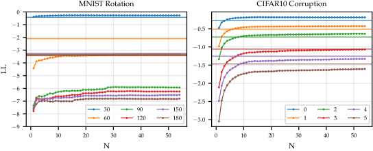
Figure 6: Rotated MNIST (left) and Corrupted CIFAR10 (right) results for deep ensembles (Lakshminarayanan et al., 2017) with large numbers of ensemble members (i.e. up to 55). Horizontal axis denotes number of ensemble members, and vertical axis denotes performance in terms of log-likelihood. Straight horizontal lines correspond to the performance of our method, as a reference. Colors denote different levels of rotation (left) and corruption (right).

A.2 Scalability of Subnetwork Linearised Laplace in the number of Weights

The aim of subnetwork inference is to scale existing posterior approximations to large networks. To further validate that this objective can be achieved, we perform subnetwork inference in ResNet50. We use a similar (slightly smaller) subnetwork size than we used with ResNet18: our subnetwork contains 39,190 / 23,466,560 ($0.167\%$) parameters. The results obtained with this model are displayed in Fig. 7. Subnetwork inference in ResNet50 improves upon a simple MAP estimate of the weights in terms of both log-likelihood and calibration metrics.

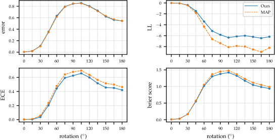
Figure 7: MNIST rotation results for ResNet-50, reporting predictive error, log-likelihood (LL), expected calibration error (ECE) and brier score. We choose a subnetwork containing only 0.167$\%$ (39,190 / 23,466,560) of the parameters of the full network.

A.3 Out-of-Distribution Rejection

In this section we provide additional results on out-of-distribution (OOD) rejection using predictive uncertainty. First, we train our models on a source dataset. We then evaluate them on the test set from our source dataset and on the test set of a target (out-of-distribution) dataset. We expect predictions for the target dataset to be more uncertain than those for the source dataset. Using predictive uncertainty as the discriminative variable we compute the area under ROC for each method under consideration and display them in Table 1. The CIFAR-SVHN and MNIST-Fashion dataset pairs are chosen following Nalisnick et al. (2019). On the CIFAR-SVHN task, all methods perform similarly, except for ensembles, which clearly does best. On MNIST-Fashion, SWAG performs best, followed by Subnetwork Linearised Laplace and ensembles.

Table 1: AUC-ROC scores for out-of-distribution detection, using CIFAR10 vs SVHN and MNIST vs FashionMNIST as in- (source) and out-of-distribution (target) datasets, respectively.

Source	Target	Ours	Ours (Rand)	Dropout	Diag-Lap	Ensemble	MAP	SWAG
CIFAR10	SVHN	$0.85\scriptstyle\pm 0.03$	$0.86\scriptstyle\pm 0.02$	$0.85\scriptstyle\pm 0.01$	$0.86\scriptstyle\pm 0.02$	$0.91\scriptstyle\pm 0.00$	$0.86\scriptstyle\pm 0.02$	$0.83\scriptstyle\pm 0.00$
MNIST	Fashion	$0.92\scriptstyle\pm 0.05$	$0.75\scriptstyle\pm 0.02$	$0.82\scriptstyle\pm 0.12$	$0.75\scriptstyle\pm 0.01$	$0.90\scriptstyle\pm 0.09$	$0.72\scriptstyle\pm 0.03$	$0.97\scriptstyle\pm 0.01$

We also simulate a realistic OOD rejection scenario (Filos et al., 2019) by jointly evaluating our models on an in-distribution and an OOD test set. We allow our methods to reject increasing proportions of the data based on predictive entropy before classifying the rest. All predictions on OOD samples are treated as incorrect. Following (Nalisnick et al., 2019), we use CIFAR10 vs SVHN and MNIST vs FashionMNIST as in- and out-of-distribution datasets, respectively. Note that the SVHN test set is randomly sub-sampled down to a size of 10,000 to match that of CIFAR10. The results are shown in Fig. 8. On CIFAR-SVHN all methods perform similarly, with exceptions being ensembles, which perform best and SWAG which does worse. On MNIST-Fashion SWAG performs best, followed by Subnetwork Linearised Laplace. All other methods fail to distinguish very uncertain in-distribution data from low uncertainty OOD points.

Figure 8: Rejection-classification plots.

A.4 Additional Rotation and Corruption Results

We complement our results from Fig. 4 in the main text with results on additional calibration metrics: ECE and Brier Score, in Fig. 9. Please refer to the appendix of (Antorán et al., 2020) for a description of these.

Figure 9: Full MNIST rotation and CIFAR10 corruption results, for ResNet-18, reporting predictive error, log-likelihood (LL), expected calibration error (ECE) and Brier score, respectively (from top to bottom).

For reference, we provide our results from Fig. 4 and Fig. 9 in numerical format in the tables below.

Table 2: MNIST – no rotation.

	Ours	Ours (Rand)	Dropout	Diag-Lap	Ensemble	MAP	SWAG	VOGN
LL	$-0.07\scriptstyle\pm 0.01$	$-0.01\scriptstyle\pm 0.00$	$-0.01\scriptstyle\pm 0.00$	$-0.04\scriptstyle\pm 0.03$	$-0.01\scriptstyle\pm 0.00$	$-0.01\scriptstyle\pm 0.00$	$-0.01\scriptstyle\pm 0.00$	$-0.14\scriptstyle\pm nan$
error	$0.01\scriptstyle\pm 0.00$	$0.00\scriptstyle\pm 0.00$	$0.00\scriptstyle\pm 0.00$	$0.01\scriptstyle\pm 0.01$	$0.00\scriptstyle\pm 0.00$	$0.00\scriptstyle\pm 0.00$	$0.00\scriptstyle\pm 0.00$	$0.01\scriptstyle\pm nan$
ECE	$0.05\scriptstyle\pm 0.01$	$0.00\scriptstyle\pm 0.00$	$0.00\scriptstyle\pm 0.00$	$0.00\scriptstyle\pm 0.00$	$0.00\scriptstyle\pm 0.00$	$0.00\scriptstyle\pm 0.00$	$0.00\scriptstyle\pm 0.00$	$0.10\scriptstyle\pm nan$
brier score	$0.02\scriptstyle\pm 0.00$	$0.01\scriptstyle\pm 0.00$	$0.01\scriptstyle\pm 0.00$	$0.02\scriptstyle\pm 0.01$	$0.01\scriptstyle\pm 0.00$	$0.01\scriptstyle\pm 0.00$	$0.01\scriptstyle\pm 0.00$	$0.04\scriptstyle\pm nan$

Table 3: MNIST – $15^{\circ}$ rotation.

	Ours	Ours (Rand)	Dropout	Diag-Lap	Ensemble	MAP	SWAG	VOGN
LL	$-0.14\scriptstyle\pm 0.02$	$-0.05\scriptstyle\pm 0.00$	$-0.05\scriptstyle\pm 0.00$	$-0.11\scriptstyle\pm 0.08$	$-0.04\scriptstyle\pm 0.00$	$-0.05\scriptstyle\pm 0.00$	$-0.04\scriptstyle\pm 0.00$	$-0.19\scriptstyle\pm nan$
error	$0.02\scriptstyle\pm 0.00$	$0.02\scriptstyle\pm 0.00$	$0.01\scriptstyle\pm 0.00$	$0.03\scriptstyle\pm 0.02$	$0.01\scriptstyle\pm 0.00$	$0.02\scriptstyle\pm 0.00$	$0.01\scriptstyle\pm 0.00$	$0.02\scriptstyle\pm nan$
ECE	$0.08\scriptstyle\pm 0.01$	$0.00\scriptstyle\pm 0.00$	$0.00\scriptstyle\pm 0.00$	$0.01\scriptstyle\pm 0.01$	$0.00\scriptstyle\pm 0.00$	$0.00\scriptstyle\pm 0.00$	$0.00\scriptstyle\pm 0.00$	$0.12\scriptstyle\pm nan$
brier score	$0.05\scriptstyle\pm 0.01$	$0.03\scriptstyle\pm 0.00$	$0.02\scriptstyle\pm 0.00$	$0.05\scriptstyle\pm 0.03$	$0.02\scriptstyle\pm 0.00$	$0.02\scriptstyle\pm 0.00$	$0.02\scriptstyle\pm 0.00$	$0.07\scriptstyle\pm nan$

Table 4: MNIST – $30^{\circ}$ rotation.

	Ours	Ours (Rand)	Dropout	Diag-Lap	Ensemble	MAP	SWAG	VOGN
LL	$-0.42\scriptstyle\pm 0.04$	$-0.36\scriptstyle\pm 0.01$	$-0.32\scriptstyle\pm 0.02$	$-0.44\scriptstyle\pm 0.06$	$-0.28\scriptstyle\pm 0.02$	$-0.39\scriptstyle\pm 0.01$	$-0.30\scriptstyle\pm 0.00$	$-0.51\scriptstyle\pm nan$
error	$0.11\scriptstyle\pm 0.01$	$0.10\scriptstyle\pm 0.00$	$0.09\scriptstyle\pm 0.01$	$0.12\scriptstyle\pm 0.01$	$0.08\scriptstyle\pm 0.01$	$0.10\scriptstyle\pm 0.00$	$0.08\scriptstyle\pm 0.00$	$0.14\scriptstyle\pm nan$
ECE	$0.10\scriptstyle\pm 0.02$	$0.04\scriptstyle\pm 0.01$	$0.03\scriptstyle\pm 0.00$	$0.06\scriptstyle\pm 0.01$	$0.02\scriptstyle\pm 0.00$	$0.05\scriptstyle\pm 0.00$	$0.04\scriptstyle\pm 0.00$	$0.13\scriptstyle\pm nan$
brier score	$0.19\scriptstyle\pm 0.02$	$0.16\scriptstyle\pm 0.00$	$0.14\scriptstyle\pm 0.01$	$0.18\scriptstyle\pm 0.02$	$0.12\scriptstyle\pm 0.01$	$0.16\scriptstyle\pm 0.00$	$0.12\scriptstyle\pm 0.00$	$0.23\scriptstyle\pm nan$

Table 5: MNIST – $45^{\circ}$ rotation.

	Ours	Ours (Rand)	Dropout	Diag-Lap	Ensemble	MAP	SWAG	VOGN
LL	$-1.09\scriptstyle\pm 0.03$	$-1.60\scriptstyle\pm 0.05$	$-1.44\scriptstyle\pm 0.11$	$-1.68\scriptstyle\pm 0.20$	$-1.36\scriptstyle\pm 0.07$	$-1.75\scriptstyle\pm 0.06$	$-1.35\scriptstyle\pm 0.02$	$-1.15\scriptstyle\pm nan$
error	$0.36\scriptstyle\pm 0.01$	$0.35\scriptstyle\pm 0.01$	$0.33\scriptstyle\pm 0.01$	$0.35\scriptstyle\pm 0.03$	$0.31\scriptstyle\pm 0.01$	$0.35\scriptstyle\pm 0.01$	$0.29\scriptstyle\pm 0.00$	$0.40\scriptstyle\pm nan$
ECE	$0.03\scriptstyle\pm 0.01$	$0.22\scriptstyle\pm 0.01$	$0.19\scriptstyle\pm 0.02$	$0.22\scriptstyle\pm 0.02$	$0.17\scriptstyle\pm 0.01$	$0.23\scriptstyle\pm 0.01$	$0.18\scriptstyle\pm 0.00$	$0.01\scriptstyle\pm nan$
brier score	$0.49\scriptstyle\pm 0.02$	$0.55\scriptstyle\pm 0.02$	$0.52\scriptstyle\pm 0.02$	$0.55\scriptstyle\pm 0.04$	$0.48\scriptstyle\pm 0.02$	$0.56\scriptstyle\pm 0.02$	$0.46\scriptstyle\pm 0.01$	$0.53\scriptstyle\pm nan$

Table 6: MNIST – $60^{\circ}$ rotation.

	Ours	Ours (Rand)	Dropout	Diag-Lap	Ensemble	MAP	SWAG	VOGN
LL	$-2.10\scriptstyle\pm 0.03$	$-3.85\scriptstyle\pm 0.18$	$-3.54\scriptstyle\pm 0.23$	$-4.11\scriptstyle\pm 0.66$	$-3.60\scriptstyle\pm 0.10$	$-4.29\scriptstyle\pm 0.21$	$-2.95\scriptstyle\pm 0.08$	$-1.92\scriptstyle\pm nan$
error	$0.63\scriptstyle\pm 0.01$	$0.63\scriptstyle\pm 0.01$	$0.62\scriptstyle\pm 0.01$	$0.62\scriptstyle\pm 0.05$	$0.61\scriptstyle\pm 0.01$	$0.63\scriptstyle\pm 0.01$	$0.53\scriptstyle\pm 0.02$	$0.64\scriptstyle\pm nan$
ECE	$0.25\scriptstyle\pm 0.02$	$0.46\scriptstyle\pm 0.02$	$0.43\scriptstyle\pm 0.02$	$0.47\scriptstyle\pm 0.06$	$0.42\scriptstyle\pm 0.01$	$0.48\scriptstyle\pm 0.02$	$0.36\scriptstyle\pm 0.02$	$0.17\scriptstyle\pm nan$
brier score	$0.85\scriptstyle\pm 0.02$	$1.04\scriptstyle\pm 0.03$	$1.00\scriptstyle\pm 0.03$	$1.05\scriptstyle\pm 0.10$	$0.98\scriptstyle\pm 0.02$	$1.07\scriptstyle\pm 0.03$	$0.86\scriptstyle\pm 0.03$	$0.80\scriptstyle\pm nan$

Table 7: MNIST – $75^{\circ}$ rotation.

	Ours	Ours (Rand)	Dropout	Diag-Lap	Ensemble	MAP	SWAG	VOGN
LL	$-3.02\scriptstyle\pm 0.07$	$-5.93\scriptstyle\pm 0.28$	$-5.49\scriptstyle\pm 0.38$	$-6.92\scriptstyle\pm 0.32$	$-5.74\scriptstyle\pm 0.15$	$-6.63\scriptstyle\pm 0.33$	$-4.46\scriptstyle\pm 0.18$	$-2.54\scriptstyle\pm nan$
error	$0.80\scriptstyle\pm 0.02$	$0.79\scriptstyle\pm 0.01$	$0.79\scriptstyle\pm 0.01$	$0.81\scriptstyle\pm 0.00$	$0.78\scriptstyle\pm 0.01$	$0.79\scriptstyle\pm 0.01$	$0.72\scriptstyle\pm 0.02$	$0.77\scriptstyle\pm nan$
ECE	$0.41\scriptstyle\pm 0.04$	$0.62\scriptstyle\pm 0.03$	$0.59\scriptstyle\pm 0.01$	$0.65\scriptstyle\pm 0.01$	$0.58\scriptstyle\pm 0.01$	$0.64\scriptstyle\pm 0.03$	$0.51\scriptstyle\pm 0.02$	$0.26\scriptstyle\pm nan$
brier score	$1.08\scriptstyle\pm 0.04$	$1.34\scriptstyle\pm 0.04$	$1.30\scriptstyle\pm 0.02$	$1.39\scriptstyle\pm 0.01$	$1.29\scriptstyle\pm 0.02$	$1.37\scriptstyle\pm 0.04$	$1.17\scriptstyle\pm 0.04$	$0.95\scriptstyle\pm nan$

Table 8: MNIST – $90^{\circ}$ rotation.

	Ours	Ours (Rand)	Dropout	Diag-Lap	Ensemble	MAP	SWAG	VOGN
LL	$-3.35\scriptstyle\pm 0.13$	$-6.46\scriptstyle\pm 0.15$	$-6.18\scriptstyle\pm 0.41$	$-7.32\scriptstyle\pm 0.67$	$-6.39\scriptstyle\pm 0.17$	$-7.18\scriptstyle\pm 0.22$	$-5.63\scriptstyle\pm 0.12$	$-2.91\scriptstyle\pm nan$
error	$0.84\scriptstyle\pm 0.02$	$0.84\scriptstyle\pm 0.01$	$0.84\scriptstyle\pm 0.01$	$0.85\scriptstyle\pm 0.01$	$0.84\scriptstyle\pm 0.01$	$0.84\scriptstyle\pm 0.01$	$0.82\scriptstyle\pm 0.02$	$0.81\scriptstyle\pm nan$
ECE	$0.43\scriptstyle\pm 0.03$	$0.64\scriptstyle\pm 0.04$	$0.62\scriptstyle\pm 0.01$	$0.66\scriptstyle\pm 0.03$	$0.62\scriptstyle\pm 0.01$	$0.66\scriptstyle\pm 0.04$	$0.60\scriptstyle\pm 0.01$	$0.29\scriptstyle\pm nan$
brier score	$1.13\scriptstyle\pm 0.03$	$1.40\scriptstyle\pm 0.05$	$1.37\scriptstyle\pm 0.01$	$1.44\scriptstyle\pm 0.04$	$1.36\scriptstyle\pm 0.01$	$1.43\scriptstyle\pm 0.05$	$1.34\scriptstyle\pm 0.02$	$1.02\scriptstyle\pm nan$

Table 9: MNIST – $105^{\circ}$ rotation.

	Ours	Ours (Rand)	Dropout	Diag-Lap	Ensemble	MAP	SWAG	VOGN
LL	$-3.59\scriptstyle\pm 0.05$	$-7.06\scriptstyle\pm 0.45$	$-6.70\scriptstyle\pm 0.52$	$-7.69\scriptstyle\pm 0.99$	$-7.01\scriptstyle\pm 0.17$	$-7.87\scriptstyle\pm 0.53$	$-6.28\scriptstyle\pm 0.19$	$-3.10\scriptstyle\pm nan$
error	$0.85\scriptstyle\pm 0.02$	$0.84\scriptstyle\pm 0.02$	$0.84\scriptstyle\pm 0.01$	$0.85\scriptstyle\pm 0.01$	$0.84\scriptstyle\pm 0.01$	$0.84\scriptstyle\pm 0.02$	$0.81\scriptstyle\pm 0.00$	$0.81\scriptstyle\pm nan$
ECE	$0.47\scriptstyle\pm 0.04$	$0.67\scriptstyle\pm 0.05$	$0.63\scriptstyle\pm 0.01$	$0.67\scriptstyle\pm 0.03$	$0.64\scriptstyle\pm 0.01$	$0.68\scriptstyle\pm 0.04$	$0.61\scriptstyle\pm 0.01$	$0.34\scriptstyle\pm nan$
brier score	$1.17\scriptstyle\pm 0.05$	$1.44\scriptstyle\pm 0.07$	$1.38\scriptstyle\pm 0.02$	$1.44\scriptstyle\pm 0.04$	$1.40\scriptstyle\pm 0.01$	$1.46\scriptstyle\pm 0.07$	$1.34\scriptstyle\pm 0.02$	$1.07\scriptstyle\pm nan$

Table 10: MNIST – $120^{\circ}$ rotation.

	Ours	Ours (Rand)	Dropout	Diag-Lap	Ensemble	MAP	SWAG	VOGN
LL	$-3.43\scriptstyle\pm 0.07$	$-6.73\scriptstyle\pm 0.53$	$-6.62\scriptstyle\pm 0.39$	$-7.92\scriptstyle\pm 0.59$	$-6.73\scriptstyle\pm 0.11$	$-7.53\scriptstyle\pm 0.63$	$-6.49\scriptstyle\pm 0.36$	$-3.07\scriptstyle\pm nan$
error	$0.80\scriptstyle\pm 0.02$	$0.79\scriptstyle\pm 0.02$	$0.78\scriptstyle\pm 0.01$	$0.81\scriptstyle\pm 0.01$	$0.78\scriptstyle\pm 0.01$	$0.79\scriptstyle\pm 0.02$	$0.76\scriptstyle\pm 0.02$	$0.76\scriptstyle\pm nan$
ECE	$0.40\scriptstyle\pm 0.03$	$0.62\scriptstyle\pm 0.05$	$0.58\scriptstyle\pm 0.01$	$0.65\scriptstyle\pm 0.04$	$0.59\scriptstyle\pm 0.01$	$0.63\scriptstyle\pm 0.04$	$0.58\scriptstyle\pm 0.03$	$0.30\scriptstyle\pm nan$
brier score	$1.10\scriptstyle\pm 0.03$	$1.35\scriptstyle\pm 0.07$	$1.29\scriptstyle\pm 0.02$	$1.39\scriptstyle\pm 0.06$	$1.30\scriptstyle\pm 0.01$	$1.36\scriptstyle\pm 0.07$	$1.27\scriptstyle\pm 0.04$	$1.04\scriptstyle\pm nan$

Table 11: MNIST – $135^{\circ}$ rotation.

	Ours	Ours (Rand)	Dropout	Diag-Lap	Ensemble	MAP	SWAG	VOGN
LL	$-3.24\scriptstyle\pm 0.06$	$-6.43\scriptstyle\pm 0.38$	$-6.46\scriptstyle\pm 0.28$	$-7.05\scriptstyle\pm 0.88$	$-6.57\scriptstyle\pm 0.10$	$-7.24\scriptstyle\pm 0.48$	$-6.40\scriptstyle\pm 0.37$	$-2.89\scriptstyle\pm nan$
error	$0.71\scriptstyle\pm 0.02$	$0.71\scriptstyle\pm 0.02$	$0.70\scriptstyle\pm 0.01$	$0.71\scriptstyle\pm 0.01$	$0.70\scriptstyle\pm 0.01$	$0.71\scriptstyle\pm 0.02$	$0.70\scriptstyle\pm 0.02$	$0.67\scriptstyle\pm nan$
ECE	$0.32\scriptstyle\pm 0.01$	$0.55\scriptstyle\pm 0.03$	$0.52\scriptstyle\pm 0.01$	$0.56\scriptstyle\pm 0.02$	$0.52\scriptstyle\pm 0.01$	$0.56\scriptstyle\pm 0.03$	$0.53\scriptstyle\pm 0.02$	$0.25\scriptstyle\pm nan$
brier score	$0.99\scriptstyle\pm 0.02$	$1.21\scriptstyle\pm 0.05$	$1.17\scriptstyle\pm 0.02$	$1.22\scriptstyle\pm 0.04$	$1.17\scriptstyle\pm 0.01$	$1.23\scriptstyle\pm 0.05$	$1.18\scriptstyle\pm 0.04$	$0.94\scriptstyle\pm nan$

Table 12: MNIST – $150^{\circ}$ rotation.

	Ours	Ours (Rand)	Dropout	Diag-Lap	Ensemble	MAP	SWAG	VOGN
LL	$-3.25\scriptstyle\pm 0.05$	$-6.56\scriptstyle\pm 0.18$	$-6.62\scriptstyle\pm 0.33$	$-7.04\scriptstyle\pm 0.36$	$-6.88\scriptstyle\pm 0.11$	$-7.41\scriptstyle\pm 0.25$	$-6.39\scriptstyle\pm 0.27$	$-2.69\scriptstyle\pm nan$
error	$0.63\scriptstyle\pm 0.02$	$0.63\scriptstyle\pm 0.01$	$0.63\scriptstyle\pm 0.00$	$0.65\scriptstyle\pm 0.01$	$0.62\scriptstyle\pm 0.01$	$0.63\scriptstyle\pm 0.01$	$0.63\scriptstyle\pm 0.01$	$0.60\scriptstyle\pm nan$
ECE	$0.29\scriptstyle\pm 0.01$	$0.50\scriptstyle\pm 0.01$	$0.48\scriptstyle\pm 0.01$	$0.52\scriptstyle\pm 0.01$	$0.48\scriptstyle\pm 0.01$	$0.51\scriptstyle\pm 0.01$	$0.49\scriptstyle\pm 0.01$	$0.23\scriptstyle\pm nan$
brier score	$0.92\scriptstyle\pm 0.02$	$1.10\scriptstyle\pm 0.02$	$1.07\scriptstyle\pm 0.01$	$1.13\scriptstyle\pm 0.02$	$1.06\scriptstyle\pm 0.01$	$1.11\scriptstyle\pm 0.02$	$1.08\scriptstyle\pm 0.02$	$0.85\scriptstyle\pm nan$

Table 13: MNIST – $165^{\circ}$ rotation.

	Ours	Ours (Rand)	Dropout	Diag-Lap	Ensemble	MAP	SWAG	VOGN
LL	$-3.42\scriptstyle\pm 0.12$	$-7.01\scriptstyle\pm 0.15$	$-7.08\scriptstyle\pm 0.39$	$-7.80\scriptstyle\pm 0.12$	$-7.51\scriptstyle\pm 0.11$	$-7.91\scriptstyle\pm 0.18$	$-6.63\scriptstyle\pm 0.24$	$-2.67\scriptstyle\pm nan$
error	$0.58\scriptstyle\pm 0.01$	$0.58\scriptstyle\pm 0.01$	$0.58\scriptstyle\pm 0.01$	$0.58\scriptstyle\pm 0.00$	$0.57\scriptstyle\pm 0.01$	$0.58\scriptstyle\pm 0.01$	$0.59\scriptstyle\pm 0.00$	$0.56\scriptstyle\pm nan$
ECE	$0.32\scriptstyle\pm 0.02$	$0.49\scriptstyle\pm 0.01$	$0.48\scriptstyle\pm 0.01$	$0.49\scriptstyle\pm 0.01$	$0.48\scriptstyle\pm 0.00$	$0.51\scriptstyle\pm 0.01$	$0.48\scriptstyle\pm 0.00$	$0.25\scriptstyle\pm nan$
brier score	$0.90\scriptstyle\pm 0.02$	$1.05\scriptstyle\pm 0.01$	$1.04\scriptstyle\pm 0.01$	$1.05\scriptstyle\pm 0.01$	$1.03\scriptstyle\pm 0.01$	$1.07\scriptstyle\pm 0.02$	$1.03\scriptstyle\pm 0.01$	$0.82\scriptstyle\pm nan$

Table 14: MNIST – $180^{\circ}$ rotation.

	Ours	Ours (Rand)	Dropout	Diag-Lap	Ensemble	MAP	SWAG	VOGN
LL	$-3.32\scriptstyle\pm 0.13$	$-6.63\scriptstyle\pm 0.18$	$-6.87\scriptstyle\pm 0.32$	$-7.10\scriptstyle\pm 0.47$	$-7.16\scriptstyle\pm 0.16$	$-7.43\scriptstyle\pm 0.20$	$-6.61\scriptstyle\pm 0.22$	$-2.71\scriptstyle\pm nan$
error	$0.56\scriptstyle\pm 0.01$	$0.56\scriptstyle\pm 0.01$	$0.56\scriptstyle\pm 0.00$	$0.55\scriptstyle\pm 0.01$	$0.55\scriptstyle\pm 0.00$	$0.56\scriptstyle\pm 0.01$	$0.57\scriptstyle\pm 0.00$	$0.55\scriptstyle\pm nan$
ECE	$0.29\scriptstyle\pm 0.02$	$0.46\scriptstyle\pm 0.01$	$0.45\scriptstyle\pm 0.00$	$0.46\scriptstyle\pm 0.00$	$0.46\scriptstyle\pm 0.01$	$0.48\scriptstyle\pm 0.01$	$0.47\scriptstyle\pm 0.01$	$0.25\scriptstyle\pm nan$
brier score	$0.86\scriptstyle\pm 0.02$	$1.00\scriptstyle\pm 0.01$	$0.99\scriptstyle\pm 0.01$	$0.99\scriptstyle\pm 0.01$	$0.99\scriptstyle\pm 0.00$	$1.01\scriptstyle\pm 0.02$	$1.01\scriptstyle\pm 0.01$	$0.82\scriptstyle\pm nan$

Table 15: CIFAR10 – no corruption.

	Ours	Ours (Rand)	Dropout	Diag-Lap	Ensemble	MAP	SWAG	VOGN
LL	$-0.27\scriptstyle\pm 0.00$	$-0.43\scriptstyle\pm 0.01$	$-0.37\scriptstyle\pm 0.01$	$-0.50\scriptstyle\pm 0.02$	$-0.21\scriptstyle\pm 0.01$	$-0.46\scriptstyle\pm 0.02$	$-0.48\scriptstyle\pm 0.01$	$-0.61\scriptstyle\pm nan$
error	$0.09\scriptstyle\pm 0.00$	$0.08\scriptstyle\pm 0.00$	$0.08\scriptstyle\pm 0.00$	$0.09\scriptstyle\pm 0.00$	$0.06\scriptstyle\pm 0.00$	$0.08\scriptstyle\pm 0.00$	$0.11\scriptstyle\pm 0.00$	$0.21\scriptstyle\pm nan$
ECE	$0.01\scriptstyle\pm 0.00$	$0.06\scriptstyle\pm 0.00$	$0.04\scriptstyle\pm 0.00$	$0.06\scriptstyle\pm 0.00$	$0.01\scriptstyle\pm 0.00$	$0.06\scriptstyle\pm 0.00$	$0.07\scriptstyle\pm 0.00$	$0.03\scriptstyle\pm nan$
brier score	$0.13\scriptstyle\pm 0.00$	$0.14\scriptstyle\pm 0.00$	$0.13\scriptstyle\pm 0.00$	$0.15\scriptstyle\pm 0.00$	$0.09\scriptstyle\pm 0.00$	$0.14\scriptstyle\pm 0.00$	$0.17\scriptstyle\pm 0.00$	$0.30\scriptstyle\pm nan$

Table 16: CIFAR10 – level $1$ corruption.

	Ours	Ours (Rand)	Dropout	Diag-Lap	Ensemble	MAP	SWAG	VOGN
LL	$-0.51\scriptstyle\pm 0.01$	$-0.91\scriptstyle\pm 0.01$	$-0.80\scriptstyle\pm 0.02$	$-1.03\scriptstyle\pm 0.02$	$-0.50\scriptstyle\pm 0.02$	$-0.96\scriptstyle\pm 0.02$	$-0.89\scriptstyle\pm 0.02$	$-0.99\scriptstyle\pm nan$
error	$0.17\scriptstyle\pm 0.01$	$0.16\scriptstyle\pm 0.00$	$0.16\scriptstyle\pm 0.00$	$0.17\scriptstyle\pm 0.00$	$0.13\scriptstyle\pm 0.00$	$0.16\scriptstyle\pm 0.00$	$0.17\scriptstyle\pm 0.00$	$0.32\scriptstyle\pm nan$
ECE	$0.03\scriptstyle\pm 0.00$	$0.11\scriptstyle\pm 0.00$	$0.10\scriptstyle\pm 0.00$	$0.13\scriptstyle\pm 0.00$	$0.04\scriptstyle\pm 0.00$	$0.12\scriptstyle\pm 0.01$	$0.11\scriptstyle\pm 0.00$	$0.03\scriptstyle\pm nan$
brier score	$0.24\scriptstyle\pm 0.00$	$0.27\scriptstyle\pm 0.00$	$0.25\scriptstyle\pm 0.00$	$0.29\scriptstyle\pm 0.00$	$0.19\scriptstyle\pm 0.00$	$0.27\scriptstyle\pm 0.01$	$0.29\scriptstyle\pm 0.00$	$0.44\scriptstyle\pm nan$

Table 17: CIFAR10 – level $2$ corruption.

	Ours	Ours (Rand)	Dropout	Diag-Lap	Ensemble	MAP	SWAG	VOGN
LL	$-0.73\scriptstyle\pm 0.01$	$-1.29\scriptstyle\pm 0.06$	$-1.20\scriptstyle\pm 0.02$	$-1.50\scriptstyle\pm 0.12$	$-0.80\scriptstyle\pm 0.01$	$-1.40\scriptstyle\pm 0.03$	$-1.21\scriptstyle\pm 0.00$	$-1.31\scriptstyle\pm nan$
error	$0.23\scriptstyle\pm 0.00$	$0.22\scriptstyle\pm 0.01$	$0.22\scriptstyle\pm 0.00$	$0.23\scriptstyle\pm 0.01$	$0.19\scriptstyle\pm 0.00$	$0.22\scriptstyle\pm 0.00$	$0.22\scriptstyle\pm 0.00$	$0.40\scriptstyle\pm nan$
ECE	$0.06\scriptstyle\pm 0.00$	$0.16\scriptstyle\pm 0.01$	$0.14\scriptstyle\pm 0.00$	$0.17\scriptstyle\pm 0.01$	$0.07\scriptstyle\pm 0.00$	$0.16\scriptstyle\pm 0.00$	$0.15\scriptstyle\pm 0.00$	$0.10\scriptstyle\pm nan$
brier score	$0.33\scriptstyle\pm 0.00$	$0.37\scriptstyle\pm 0.01$	$0.35\scriptstyle\pm 0.01$	$0.40\scriptstyle\pm 0.02$	$0.28\scriptstyle\pm 0.00$	$0.37\scriptstyle\pm 0.01$	$0.37\scriptstyle\pm 0.00$	$0.56\scriptstyle\pm nan$

Table 18: CIFAR10 – level $3$ corruption.

	Ours	Ours (Rand)	Dropout	Diag-Lap	Ensemble	MAP	SWAG	VOGN
LL	$-1.06\scriptstyle\pm 0.02$	$-2.06\scriptstyle\pm 0.12$	$-1.85\scriptstyle\pm 0.07$	$-2.13\scriptstyle\pm 0.17$	$-1.28\scriptstyle\pm 0.03$	$-2.18\scriptstyle\pm 0.08$	$-1.63\scriptstyle\pm 0.03$	$-1.83\scriptstyle\pm nan$
error	$0.32\scriptstyle\pm 0.01$	$0.31\scriptstyle\pm 0.01$	$0.31\scriptstyle\pm 0.01$	$0.31\scriptstyle\pm 0.01$	$0.28\scriptstyle\pm 0.00$	$0.31\scriptstyle\pm 0.01$	$0.28\scriptstyle\pm 0.00$	$0.51\scriptstyle\pm nan$
ECE	$0.11\scriptstyle\pm 0.01$	$0.24\scriptstyle\pm 0.01$	$0.21\scriptstyle\pm 0.01$	$0.24\scriptstyle\pm 0.01$	$0.12\scriptstyle\pm 0.00$	$0.24\scriptstyle\pm 0.01$	$0.20\scriptstyle\pm 0.00$	$0.19\scriptstyle\pm nan$
brier score	$0.46\scriptstyle\pm 0.01$	$0.54\scriptstyle\pm 0.02$	$0.50\scriptstyle\pm 0.02$	$0.54\scriptstyle\pm 0.03$	$0.42\scriptstyle\pm 0.00$	$0.54\scriptstyle\pm 0.02$	$0.47\scriptstyle\pm 0.01$	$0.72\scriptstyle\pm nan$

Table 19: CIFAR10 – level $4$ corruption.

	Ours	Ours (Rand)	Dropout	Diag-Lap	Ensemble	MAP	SWAG	VOGN
LL	$-1.25\scriptstyle\pm 0.03$	$-2.43\scriptstyle\pm 0.18$	$-2.28\scriptstyle\pm 0.10$	$-2.54\scriptstyle\pm 0.18$	$-1.56\scriptstyle\pm 0.05$	$-2.57\scriptstyle\pm 0.15$	$-1.95\scriptstyle\pm 0.04$	$-1.99\scriptstyle\pm nan$
error	$0.36\scriptstyle\pm 0.01$	$0.35\scriptstyle\pm 0.01$	$0.35\scriptstyle\pm 0.01$	$0.35\scriptstyle\pm 0.01$	$0.32\scriptstyle\pm 0.01$	$0.35\scriptstyle\pm 0.01$	$0.32\scriptstyle\pm 0.00$	$0.54\scriptstyle\pm nan$
ECE	$0.13\scriptstyle\pm 0.01$	$0.27\scriptstyle\pm 0.01$	$0.24\scriptstyle\pm 0.01$	$0.27\scriptstyle\pm 0.01$	$0.14\scriptstyle\pm 0.01$	$0.27\scriptstyle\pm 0.02$	$0.23\scriptstyle\pm 0.00$	$0.22\scriptstyle\pm nan$
brier score	$0.51\scriptstyle\pm 0.02$	$0.60\scriptstyle\pm 0.03$	$0.57\scriptstyle\pm 0.01$	$0.61\scriptstyle\pm 0.02$	$0.47\scriptstyle\pm 0.01$	$0.60\scriptstyle\pm 0.03$	$0.53\scriptstyle\pm 0.00$	$0.76\scriptstyle\pm nan$

Table 20: CIFAR10 – level $5$ corruption.

	Ours	Ours (Rand)	Dropout	Diag-Lap	Ensemble	MAP	SWAG	VOGN
LL	$-1.47\scriptstyle\pm 0.03$	$-2.82\scriptstyle\pm 0.11$	$-2.71\scriptstyle\pm 0.13$	$-3.20\scriptstyle\pm 0.13$	$-1.88\scriptstyle\pm 0.05$	$-3.03\scriptstyle\pm 0.10$	$-2.31\scriptstyle\pm 0.09$	$-2.00\scriptstyle\pm nan$
error	$0.41\scriptstyle\pm 0.00$	$0.40\scriptstyle\pm 0.01$	$0.40\scriptstyle\pm 0.01$	$0.41\scriptstyle\pm 0.01$	$0.37\scriptstyle\pm 0.01$	$0.40\scriptstyle\pm 0.00$	$0.36\scriptstyle\pm 0.01$	$0.54\scriptstyle\pm nan$
ECE	$0.16\scriptstyle\pm 0.01$	$0.31\scriptstyle\pm 0.01$	$0.28\scriptstyle\pm 0.01$	$0.33\scriptstyle\pm 0.02$	$0.17\scriptstyle\pm 0.01$	$0.31\scriptstyle\pm 0.01$	$0.27\scriptstyle\pm 0.01$	$0.19\scriptstyle\pm nan$
brier score	$0.58\scriptstyle\pm 0.00$	$0.69\scriptstyle\pm 0.01$	$0.65\scriptstyle\pm 0.01$	$0.72\scriptstyle\pm 0.03$	$0.55\scriptstyle\pm 0.01$	$0.69\scriptstyle\pm 0.01$	$0.61\scriptstyle\pm 0.01$	$0.75\scriptstyle\pm nan$

Appendix B Derivations for the Wasserstein Pruning Objective

B.1 Derivation for Eq. 22

Note that, for our linearized model (described in Section 3), the true posterior $p({\mathbf{w}}|\mathcal{D})$ is either Gaussian or approximately Gaussian. Additionally, the approximate posterior $q_{S}({\mathbf{w}})=q({\mathbf{w}}_{S})\ \prod_{r}\delta({\textnormal{w}}_{r}-\widehat{{\textnormal{w}}}_{r})$ can be seen as a degenerate Gaussian in which rows and columns of the covariance matrix are zeroed out. Thus, we consider the squared 2-Wasserstein distance between two Gaussian distributions $\mathcal{N}({\bm{\mu}}_{1},{\bm{\Sigma}}_{1})$ and $\mathcal{N}({\bm{\mu}}_{2},{\bm{\Sigma}}_{2})$, which has the following closed-form expression (Givens et al., 1984):

$$W_{2}\left(\mathcal{N}\left({\bm{\mu}}_{1},{\bm{\Sigma}}_{1}\right),\mathcal{N}\left({\bm{\mu}}_{2},{\bm{\Sigma}}_{2}\right)\right)^{2}=\|{\bm{\mu}}_{1}-{\bm{\mu}}_{2}\|_{2}^{2}+\text{Tr}\left({\bm{\Sigma}}_{1}+{\bm{\Sigma}}_{2}-2\left({\bm{\Sigma}}_{2}^{1/2}{\bm{\Sigma}}_{1}{\bm{\Sigma}}_{2}^{1/2}\right)^{1/2}\right)\ .$$ (24)

In this case both distributions have the same mean: ${\bm{\mu}}_{1}={\bm{\mu}}_{2}=\widehat{{\mathbf{w}}}$. The true posterior’s covariance matrix is the inverse GGN matrix, i.e. ${\bm{\Sigma}}_{1}=\widetilde{{\mathbf{H}}}^{-1}$. For the approximate posterior ${\bm{\Sigma}}_{2}=\widetilde{{\mathbf{H}}}_{S+}^{-1}$, which is equal to $\widetilde{{\mathbf{H}}}_{S}^{-1}$ (the inverse GGN matrix of the subnetwork) padded with zeros at the positions corresponding to point estimated weights ${\textnormal{w}}_{r}$, matching the shape of $\widetilde{{\mathbf{H}}}^{-1}$. Alternatively, but equivalently, we can define $\widetilde{{\mathbf{H}}}_{S+}^{-1}={\mathbf{M}}_{S}\odot\widetilde{{\mathbf{H}}}^{-1}$, where $\odot$ is the Hadamard product, and ${\mathbf{M}}_{S}$ is a mask matrix with zeros in the rows and columns corresponding to ${\textnormal{w}}_{r}$, i.e. the rows and columns corresponding to weights not included in the subnetwork. This gives us:

$$W_{2}(p({\mathbf{w}}|\mathcal{D}),q_{S}({\mathbf{w}}))^{2}$$

$$=W_{2}\left(\mathcal{N}(\widehat{{\mathbf{w}}},\widetilde{{\mathbf{H}}}^{-1}),\mathcal{N}(\widehat{{\mathbf{w}}},\widetilde{{\mathbf{H}}}_{S+}^{-1})\right)^{2}$$

$$=\cancel{\|\widehat{{\mathbf{w}}}-\widehat{{\mathbf{w}}}\|_{2}^{2}}+\text{Tr}\left(\widetilde{{\mathbf{H}}}^{-1}+\widetilde{{\mathbf{H}}}_{S+}^{-1}-2\left(\widetilde{{\mathbf{H}}}_{S+}^{-1/2}\widetilde{{\mathbf{H}}}^{-1}\widetilde{{\mathbf{H}}}_{S+}^{-1/2}\right)^{1/2}\right)$$

$$=\text{Tr}\left(\widetilde{{\mathbf{H}}}^{-1}+\widetilde{{\mathbf{H}}}_{S+}^{-1}-2\left(\widetilde{{\mathbf{H}}}_{S+}^{-1/2}\widetilde{{\mathbf{H}}}^{-1}\widetilde{{\mathbf{H}}}_{S+}^{-1/2}\right)^{1/2}\right)\ .$$

B.2 Derivation for Eq. 23

For $\widetilde{{\mathbf{H}}}^{-1}=\text{diag}(\sigma_{1}^{2},\ldots,\sigma_{D}^{2})$, the Wasserstein pruning objective in Eq. 22 simplifies to

$$W_{2}(p({\mathbf{w}}|\mathcal{D}),q_{S}({\mathbf{w}}))^{2}$$

$$=\text{Tr}\left(\widetilde{{\mathbf{H}}}^{-1}\right)+\text{Tr}\left(\widetilde{{\mathbf{H}}}_{S+}^{-1}\right)-2\text{Tr}\left(\widetilde{{\mathbf{H}}}^{-1/2}\widetilde{{\mathbf{H}}}_{S+}^{-1/2}\right)$$

$$=\sum_{d=1}^{D}\sigma_{d}^{2}+m_{d}\sigma_{d}^{2}-2m_{d}\sigma_{d}^{2}$$

$$=\sum_{d=1}^{D}\sigma_{d}^{2}(1-m_{d})\ ,$$

where $m_{d}$ is the $d^{\text{th}}$ diagonal element of ${\mathbf{M}}_{S}$, i.e. $m_{d}=1$ if ${\textnormal{w}}_{d}$ is included in the subnetwork or 0 otherwise.

Appendix C Updating the prior precision for uncertainty estimation with subnetworks

As described in Section 3, the linearised Laplace method can be understood as approximating our NN with a basis function linear model, where the jacobian of the NN evaluated at $\mathbf{x}$, $\mathbf{J}(\mathbf{x})\in\mathcal{R}^{O\times D}$ represents the feature expansion. When employing an Isotropic Gaussian prior with precision $\lambda$ and for a given output dimension $i$, this formulation corresponds to a Gaussian process with kernel

$$k_{i}(\mathbf{x},\mathbf{x}^{\prime})=\lambda^{-1}\mathbf{J}(\mathbf{x})_{i}\mathbf{J}(\mathbf{x}^{\prime})_{i}^{\top}=\lambda^{-1}\sum_{d=1}^{D}\mathbf{J}(\mathbf{x})_{i,d}\mathbf{J}(\mathbf{x}^{\prime})_{i,d}.$$ (25)

For our subnetwork model, the Jacobian feature expansion is $\mathbf{J}_{S}(\mathbf{x})\in\mathcal{R}^{O\times S}$, which is a submatrix of $\mathbf{J}(\mathbf{x})$. It follows that the implied kernel will be computed in the same way as Eq. 25, removing $D-S$ terms from the sum. The updated prior precision $\lambda_{S}=\lambda\!\cdot\!\nicefrac{{S}}{{D}}$ aims to maintain the magnitude of the sum, thus making the kernel corresponding to the subnetwork as similar as possible to that of the full network.

Appendix D Experimental Setup

D.1 Toy Experiments

We train a single, 2 hidden layer network, with 50 hidden ReLU units per layer using MAP inference until convergence. Specifically, we use SGD with a learning rate of $1\times 10^{-3}$, momentum of $0.9$ and weight decay of $1\times 10^{-4}$. We use a batch size of 512. The objective we optimise is the Gaussian log-likelihood of our data, where the mean is outputted by the network and the the variance is a hyperparameter learnt jointly with NN parameters by SGD. This variance parameters is shared among all datapoints. Once the network is trained, we perform post-hoc inference on it using different approaches. Since all of these involve the linearized approximation, the mean prediction is the same for all methods. Only their uncertainty estimates vary.

Note that while for this toy example, we could in principle use the full covariance matrix for the purpose of subnetwork selection, we still just use its diagonal (as described in Section 5) for consistency. We use GGN Laplace inference over network weights (not biases) in combination with the linearized predictive distribution in Eq. 12. Thus, all approaches considered share their predictive mean, allowing us to better compare their uncertainty estimates.

All approaches share a single prior precision of $\lambda=3$, scaled as $\lambda_{S}=\lambda\cdot\nicefrac{{S}}{{D}}$. We choose this prior precision such that the full covariance approach (optimistic baseline), where $\lambda_{S}=\lambda$, presents reasonable results. We first tried a precision of 1 and found the full covariance approach to produce excessively large errorbars (covering the whole plot). A value of 3 produces more reasonable results.

Final layer inference is performed by computing the full Laplace covariance matrix and discarding all entries except those corresponding to the final layer of the NN. Results for random sub-network selection are obtained with a single sample from a scaled uniform distribution over weight choice.

D.2 UCI Experiments

In this experiment, our fully connected NNs have numbers of hidden layers $h_{d}{=}\{1,2\}$ and hidden layer widths $w_{d}{=}\{50,100\}$. For a dataset with input dimension $i_{d}$, the number of weights is given by $D{=}(i_{d}{+}1)w_{d}{+}(h_{d}{-}1)w_{d}^{2}$. Our 2 hidden layer, 100 hidden unit models have a weight count of the order $10^{4}$. The non-linearity used is ReLU.

We first obtain a MAP estimate of each model’s weights. Specifically, we use SGD with a learning rate of $1\times 10^{-3}$, momentum of $0.9$ and weight decay of $1\times 10^{-4}$. We use a batch size of 512. The objective we optimise is the Gaussian log-likelihood of our data, where the mean is outputted by the network and the the variance is a hyperparameter learnt jointly with NN parameters by SGD.

For each dataset split, we set aside 15% of the train data as a validation set. We use these for early stopping training. Training runs for a maximum of 2000 epochs but early stops with a patience of 500 if validation performance does not increase. For the larger Protein dataset, these values are 500 and 125. The weight settings which provide best validation performance are kept.

We then perform full network GGN Laplace inference for each model. We also use our proposed Wassertein rule together with the diagonal Hessian assumption to prune every network’s weight variances such that the number of variances that remain matches the size of every smaller network under consideration. The prior precision used for these steps is chosen such that the resulting predictor’s logliklihood performance on the validation set is maximised. Specifically, we employ a grid search over the values: $\lambda:[0.0001,0.001,0.1,0.5,1,2,5,10,100,1000]$. In all cases, we employ the linearized predictive in Eq. 12. Consequently, networks with the same number of weights make the same mean predictions. Increasing the number of weight variances considered will thus only increase predictive uncertainty.

D.3 Image Experiments

The results shown in Section 6.3 and Appendix A are obtained by training ResNet-18 (and ResNet-50) models using SGD with momentum. For each experiment repetition, we train 7 different models: The first is for: ‘MAP’, ‘Ours’, ‘Ours (Rand)’, ‘SWAG’, ‘Diag-Laplace’ and as the first element of ‘Ensemble’. We train 4 additional ‘Ensemble’ elements, 1 network with ‘Dropout’, and, finally 1 network for ‘VOGN’. The methods ‘Ours’, ‘Ours (Rand)’, ‘SWAG’, and ‘Diag-Laplace’ are applied post training.

For all methods except ‘VOGN’ we use the following training procedure. The (initial) learning rate, momentum, and weight decay are 0.1, 0.9, and $1\times 10^{-4}$, respectively. For ‘MAP’ we use 4 Nvidia P100 GPUs with a total batch size of 2048. For the calculation of the Jacobian in the subnetwork selection phase we use a single P100 GPU with a batch size of 4. For the calculation of the hessian we use a single P100 GPU with a batch size of 2. We train on 1 Nvidia P100 GPU with a batch size of 256 for all other methods. Each dataset is trained for a different number of epochs, shown in Table 21. We decay the learning rate by a factor of 10 at scheduled epochs, also shown in Table 21. Otherwise, all methods and datasets share hyperparameters. These hyperparameter settings are the defaults provided by PyTorch for training on ImageNet. We found them to perform well across the board. We report results obtained at the final training epoch. We do not use a separate validation set to determine the best epoch as we found ResNet-18 and ResNet-50 to not overfit with the chosen schedules.

Table 21: Per-dataset training configuration for image experiments.

Dataset	No. Epochs	LR Schedule
MNIST	90	40, 70
CIFAR10	300	150, 225

For ‘Dropout’, we add dropout to the standard ResNet-50 model (He et al., 2016) in between the 2 and 3 convolutions in the bottleneck blocks. This approach follows Zagoruyko & Komodakis (2016) and Ashukha et al. (2020) who add dropout in-between the two convolutions of a WideResNet-50’s basic block. Following Antorán et al. (2020), we choose a dropout probability of 0.1, as they found it to perform better than the value of 0.3 suggested by Ashukha et al. (2020). We use 16 MC samples for predictions. ‘Ensemble’ uses 5 elements for prediction. Ensemble elements differ from each other in their initialisation, which is sampled from the He initialisation distribution (He et al., 2015). We do not use adversarial training as, inline with Ashukha et al. (2020), we do not find it to improve results. For ‘VOGN’ we use the same procedure and hyper-parameters as used by Osawa et al. (2019) in their CIFAR10 experiments, with the exception that we use a learning rate of $1\times 10^{-3}$ as we we found a value of $1\times 10^{-4}$ not to result in convergence. We train on a single Nvidia P100 GPU with a batch size of 256. See the authors’ GitHub for more details: github.com/team-approx-bayes/dl-with-bayes/blob/master/distributed/classification/configs/cifar10/resnet18_vogn_bs256_8gpu.json.

We modify the standard ResNet-50 and ResNet-18 architectures such that the first $7\times 7$ convolution is replaced with a $3\times 3$ convolution. Additionally, we remove the first max-pooling layer. Following (Goyal et al., 2017), we zero-initialise the last batch normalisation layer in residual blocks so that they act as identity functions at the start of training.

At test time, we tune the prior precision used for ‘Ours’, ‘Diag-Laplace’ and ‘SWAG’ approximation on a validation set for each approach individually, as in Ritter et al. (2018); Kristiadi et al. (2020). We use a grid search from $1\times 10^{-4}$ to $1\times 10^{4}$ in logarithmic steps, and then a second, finer-grained grid search between the two best performing values (again with logarithmic steps).

D.4 Datasets

The 1d toy dataset used in Section 6.1 was taken from (Antorán et al., 2020). We obtained it from the authors’ github repo: https://github.com/cambridge-mlg/DUN. Table 22 summarises the datasets used in Section 6.2.

We employ the Wine, Kin8nm and Protein datasets, together with their gap variants, because we find our models’ performance to be most dependent on the quality of the estimated uncertainty here. On most other commonly used UCI regression datasets (Hernández-Lobato & Adams, 2015) we find increased uncertainty to hurt LL performance. In other words, the predictions made when using the MAP setting of the weights are better than those from any Bayesian ensemble.

Wine and Protein are available from the UCI dataset repository (Dua & Graff, 2017). Kin8nm is available from https://www.openml.org/d/189 (Foong et al., 2019b). For the standard splits (Hernández-Lobato & Adams, 2015) 90% of the data is used for training and 10% for validation. For the gap splits (Foong et al., 2019b) a split is obtained per input dimension by ordering points by their values across that dimension and removing the middle 33% of the points. These are used for validation.

The datasets used for our image experiments are outlined in Table 23.

Table 22: Datasets from tabular regression used in Section 6.2

Dataset	N Train	N Val (15% train)	N Test	Splits	Output Dim	Output Type	Input Dim	Input Type
Wine	1223	216	160	20	1	Continous	11	Continous
Wine Gap	906	161	532	11	1	Continous	11	Continous
Kin8nm	6267	1106	819	20	1	Continous	8	Continous
Kin8nm Gap	4642	820	2730	8	1	Continous	8	Continous
Protein	34983	6174	4573	5	1	Continous	9	Continous
Protein Gap	25913	4573	15244	9	1	Continous	9	Continous

Table 23: Summary of image datasets. The test and train set sizes are shown in brackets, e.g. (test & train).

Name	Size	Input Dim.	No. Classes	No. Splits
MNIST (LeCun et al., 1998)	70,000 (60,000 & 10,000)	784 ($28\,\times\,28$)	10	2
Fashion-MNIST (Xiao et al., 2017)	70,000 (60,000 & 10,000)	784 ($28\,\times\,28$)	10	2
CIFAR10 (Krizhevsky & Hinton, 2009)	60,000 (50,000 & 10,000)	3072 ($32\,\times\,32\,\times\,3$)	10	2
SVHN (Netzer et al., 2011)	99,289 (73,257 & 26,032)	3072 ($32\,\times\,32\,\times\,3$)	10	2

References

- Amodei et al. (2016) Amodei, D., Olah, C., Steinhardt, J., Christiano, P., Schulman, J., and Mané, D. Concrete Problems in AI Safety. arXiv preprint arXiv:1606.06565, 2016.
- Antorán et al. (2020) Antorán, J., Allingham, J. U., and Hernández-Lobato, J. M. Depth Uncertainty in Neural Networks. In NeurIPS, 2020.
- Ashukha et al. (2020) Ashukha, A., Lyzhov, A., Molchanov, D., and Vetrov, D. P. Pitfalls of In-Domain Uncertainty Estimation and Ensembling in Deep Learning. In ICLR, 2020.
- Betancourt (2015) Betancourt, M. The Fundamental Incompatibility of Scalable Hamiltonian Monte Carlo and Naive Data Subsampling. In ICML, 2015.
- Bhatt et al. (2020) Bhatt, U., Zhang, Y., Antorán, J., Liao, Q. V., Sattigeri, P., Fogliato, R., Melançon, G. G., Krishnan, R., Stanley, J., Tickoo, O., et al. Uncertainty as a Form of Transparency: Measuring, Communicating, and Using Uncertainty. arXiv preprint arXiv:2011.07586, 2020.
- Bishop (2006) Bishop, C. M. Pattern recognition and machine learning. Springer, 2006.
- Blundell et al. (2015) Blundell, C., Cornebise, J., Kavukcuoglu, K., and Wierstra, D. Weight Uncertainty in Neural Networks. In ICML, 2015.
- Burt et al. (2020) Burt, D. R., Ober, S. W., Garriga-Alonso, A., and van der Wilk, M. Understanding variational inference in function-space. In Symposium on Advances in Approximate Bayesian Inference (AABI), 2020.
- Cheng et al. (2017) Cheng, Y., Wang, D., Zhou, P., and Zhang, T. A survey of model compression and acceleration for deep neural networks. arXiv preprint arXiv:1710.09282, 2017.
- Daxberger et al. (2021) Daxberger, E., Kristiadi, A., Immer, A., Eschenhagen, R., Bauer, M., and Hennig, P. Laplace Redux–Effortless Bayesian Deep Learning. In NeurIPS, 2021.
- Deng et al. (2009) Deng, J., Dong, W., Socher, R., Li, L., Kai Li, and Li Fei-Fei. Imagenet: A large-scale hierarchical image database. In CVPR, 2009.
- Denker & LeCun (1990) Denker, J. S. and LeCun, Y. Transforming neural-net output levels to probability distributions. In NIPS, 1990.
- Dua & Graff (2017) Dua, D. and Graff, C. UCI machine learning repository, 2017.
- Dusenberry et al. (2020) Dusenberry, M. W., Jerfel, G., Wen, Y., Ma, Y.-a., Snoek, J., Heller, K., Lakshminarayanan, B., and Tran, D. Efficient and scalable bayesian neural nets with rank-1 factors. In ICML, 2020.
- Eschenhagen et al. (2021) Eschenhagen, R., Daxberger, E., Hennig, P., and Kristiadi, A. Mixtures of Laplace Approximations for Improved Post-Hoc Uncertainty in Deep Learning. NeurIPS Workshop on Bayesian Deep Learning, 2021.
- Farquhar et al. (2020) Farquhar, S., Smith, L., and Gal, Y. Liberty or depth: Deep bayesian neural nets do not need complex weight posterior approximations. In NeurIPS, 2020.
- Filos et al. (2019) Filos, A., Farquhar, S., Gomez, A. N., Rudner, T. G., Kenton, Z., Smith, L., Alizadeh, M., de Kroon, A., and Gal, Y. Benchmarking bayesian deep learning with diabetic retinopathy diagnosis. In NeurIPS Workshop on Bayesian Deep Learning, 2019.
- Foong et al. (2019a) Foong, A. Y., Burt, D. R., Li, Y., and Turner, R. E. On the expressiveness of approximate inference in bayesian neural networks. In NeurIPS, 2019a.
- Foong et al. (2019b) Foong, A. Y., Li, Y., Hernández-Lobato, J. M., and Turner, R. E. In-between uncertainty in bayesian neural networks. In ICML Workshop on Uncertainty and Robustness in Deep Learning, 2019b.
- Fort et al. (2019) Fort, S., Hu, H., and Lakshminarayanan, B. Deep ensembles: A loss landscape perspective. arXiv preprint arXiv:1912.02757, 2019.
- Frankle & Carbin (2019) Frankle, J. and Carbin, M. The lottery ticket hypothesis: Finding sparse, trainable neural networks. In ICLR, 2019.
- Gal & Ghahramani (2016) Gal, Y. and Ghahramani, Z. Dropout as a bayesian approximation: Representing model uncertainty in deep learning. In ICML, 2016.
- Ghahramani (2015) Ghahramani, Z. Probabilistic machine learning and artificial intelligence. Nature, 521(7553):452–459, 2015.
- Gibbs (1998) Gibbs, M. N. Bayesian Gaussian processes for regression and classification. PhD thesis, University of Cambridge, 1998.
- Givens et al. (1984) Givens, C. R., Shortt, R. M., et al. A class of wasserstein metrics for probability distributions. The Michigan Mathematical Journal, 31(2):231–240, 1984.
- Goodfellow et al. (2016) Goodfellow, I., Bengio, Y., Courville, A., and Bengio, Y. Deep learning, volume 1. MIT Press, 2016.
- Goyal et al. (2017) Goyal, P., Dollár, P., Girshick, R., Noordhuis, P., Wesolowski, L., Kyrola, A., Tulloch, A., Jia, Y., and He, K. Accurate, large minibatch sgd: Training imagenet in 1 hour. arXiv preprint arXiv:1706.02677, 2017.
- Guo et al. (2017) Guo, C., Pleiss, G., Sun, Y., and Weinberger, K. Q. On calibration of modern neural networks. In ICML, 2017.
- He et al. (2015) He, K., Zhang, X., Ren, S., and Sun, J. Delving deep into rectifiers: Surpassing human-level performance on ImageNet classification. In ICCV, 2015.
- He et al. (2016) He, K., Zhang, X., Ren, S., and Sun, J. Deep residual learning for image recognition. In CVPR, 2016.
- Hendrycks & Dietterich (2019) Hendrycks, D. and Dietterich, T. Benchmarking neural network robustness to common corruptions and perturbations. In ICLR, 2019.
- Hernández-Lobato & Adams (2015) Hernández-Lobato, J. M. and Adams, R. Probabilistic backpropagation for scalable learning of bayesian neural networks. In ICML, 2015.
- Immer et al. (2021a) Immer, A., Bauer, M., Fortuin, V., Rätsch, G., and Khan, M. E. Scalable marginal likelihood estimation for model selection in deep learning. In ICML, 2021a.
- Immer et al. (2021b) Immer, A., Korzepa, M., and Bauer, M. Improving predictions of bayesian neural networks via local linearization. In AISTATS, 2021b.
- Izmailov et al. (2019) Izmailov, P., Maddox, W. J., Kirichenko, P., Garipov, T., Vetrov, D., and Wilson, A. G. Subspace inference for bayesian deep learning. In UAI, 2019.
- Izmailov et al. (2021) Izmailov, P., Vikram, S., Hoffman, M. D., and Wilson, A. G. What are bayesian neural network posteriors really like? In ICML, 2021.
- Khan et al. (2018) Khan, M. E., Nielsen, D., Tangkaratt, V., Lin, W., Gal, Y., and Srivastava, A. Fast and scalable bayesian deep learning by weight-perturbation in adam. In ICML, 2018.
- Khan et al. (2019) Khan, M. E. E., Immer, A., Abedi, E., and Korzepa, M. Approximate inference turns deep networks into gaussian processes. In NeurIPS, 2019.
- Kirkpatrick et al. (2017) Kirkpatrick, J., Pascanu, R., Rabinowitz, N., Veness, J., Desjardins, G., Rusu, A. A., Milan, K., Quan, J., Ramalho, T., Grabska-Barwinska, A., Hassabis, D., Clopath, C., Kumaran, D., and Hadsell, R. Overcoming catastrophic forgetting in neural networks. Proceedings of the National Academy of Sciences, 114(13):3521–3526, 2017.
- Kristiadi et al. (2020) Kristiadi, A., Hein, M., and Hennig, P. Being Bayesian, Even Just a Bit, Fixes Overconfidence in ReLU Networks. In ICML, 2020.
- Kristiadi et al. (2021) Kristiadi, A., Hein, M., and Hennig, P. Learnable Uncertainty under Laplace Approximations. In UAI, 2021.
- Krizhevsky & Hinton (2009) Krizhevsky, A. and Hinton, G. Learning Multiple Layers of Features from Tiny Images. Technical report, University of Toronto, 2009.
- Lakshminarayanan et al. (2017) Lakshminarayanan, B., Pritzel, A., and Blundell, C. Simple and scalable predictive uncertainty estimation using deep ensembles. In NIPS, 2017.
- Lawrence (2001) Lawrence, N. D. Variational inference in probabilistic models. PhD thesis, University of Cambridge, 2001.
- LeCun et al. (1998) LeCun, Y., Bottou, L., Bengio, Y., and Haffner, P. Gradient-based learning applied to document recognition. Proceedings of the IEEE, 86(11):2278–2324, 1998.
- Liu et al. (2019) Liu, X., Deng, Z., and Yang, Y. Recent progress in semantic image segmentation. Artificial Intelligence Review, 52(2):1089–1106, 2019.
- Lobacheva et al. (2020) Lobacheva, E., Chirkova, N., Kodryan, M., and Vetrov, D. P. On power laws in deep ensembles. In NeurIPS, 2020.
- Louizos & Welling (2016) Louizos, C. and Welling, M. Structured and efficient variational deep learning with matrix gaussian posteriors. In ICML, 2016.
- MacKay (1992) MacKay, D. J. A practical bayesian framework for backpropagation networks. Neural computation, 4(3):448–472, 1992.
- Maddox et al. (2019) Maddox, W. J., Izmailov, P., Garipov, T., Vetrov, D. P., and Wilson, A. G. A simple baseline for bayesian uncertainty in deep learning. In NeurIPS, 2019.
- Maddox et al. (2020) Maddox, W. J., Benton, G., and Wilson, A. G. Rethinking parameter counting in deep models: Effective dimensionality revisited. arXiv preprint arXiv:2003.02139, 2020.
- Martens (2016) Martens, J. Second-order optimization for neural networks. PhD thesis, University of Toronto, 2016.
- Martens (2020) Martens, J. New insights and perspectives on the natural gradient method. Journal of Machine Learning Research, 21(146):1–76, 2020.
- Martens & Sutskever (2011) Martens, J. and Sutskever, I. Learning recurrent neural networks with hessian-free optimization. In ICML, 2011.
- Mishkin et al. (2018) Mishkin, A., Kunstner, F., Nielsen, D., Schmidt, M., and Khan, M. E. Slang: Fast structured covariance approximations for bayesian deep learning with natural gradient. In NeurIPS, 2018.
- Nalisnick et al. (2019) Nalisnick, E., Matsukawa, A., Whye Teh, Y., Gorur, D., and Lakshminarayanan, B. Do Deep Generative Models Know What They Don’t Know? In ICLR, 2019.
- Nalisnick & Smyth (2018) Nalisnick, E. T. and Smyth, P. Learning priors for invariance. In AISTATS, 2018.
- Nalisnick et al. (2021) Nalisnick, E. T., Gordon, J., and Hernández-Lobato, J. M. Predictive complexity priors. In AISTATS, 2021.
- Neal (1995) Neal, R. M. Bayesian Learning for Neural Networks. PhD thesis, University of Toronto, 1995.
- Netzer et al. (2011) Netzer, Y., Wang, T., Coates, A., Bissacco, A., Wu, B., and Ng, A. Y. Reading Digits in Natural Images with Unsupervised Feature Learning. In NIPS Workshop on Deep Learning and Unsupervised Feature Learning, 2011.
- Nguyen et al. (2015) Nguyen, A., Yosinski, J., and Clune, J. Deep neural networks are easily fooled: High confidence predictions for unrecognizable images. In CVPR, 2015.
- Ober & Rasmussen (2019) Ober, S. W. and Rasmussen, C. E. Benchmarking the neural linear model for regression. In Symposium on Advances in Approximate Bayesian Inference (AABI), 2019.
- Osawa et al. (2019) Osawa, K., Swaroop, S., Jain, A., Eschenhagen, R., Turner, R. E., Yokota, R., and Khan, M. E. Practical deep learning with Bayesian principles. In NeurIPS, 2019.
- Ovadia et al. (2019) Ovadia, Y., Fertig, E., Lakshminarayanan, B., Nowozin, S., Sculley, D., Dillon, J., Ren, J., Nado, Z., and Snoek, J. Can you trust your model’s uncertainty? evaluating predictive uncertainty under dataset shift. In NeurIPS, 2019.
- Pearce et al. (2019) Pearce, T., Tsuchida, R., Zaki, M., Brintrup, A., and Neely, A. Expressive priors in bayesian neural networks: Kernel combinations and periodic functions. In AISTATS, 2019.
- Pinsler et al. (2019) Pinsler, R., Gordon, J., Nalisnick, E., and Hernández-Lobato, J. M. Bayesian batch active learning as sparse subset approximation. In NeurIPS, 2019.
- Riquelme et al. (2018) Riquelme, C., Tucker, G., and Snoek, J. Deep bayesian bandits showdown: An empirical comparison of bayesian deep networks for thompson sampling. In ICLR, 2018.
- Ritter et al. (2018) Ritter, H., Botev, A., and Barber, D. A scalable laplace approximation for neural networks. In ICLR, 2018.
- Rossi et al. (2020) Rossi, S., Marmin, S., and Filippone, M. Walsh-hadamard variational inference for bayesian deep learning. In NeurIPS, 2020.
- Snoek et al. (2015) Snoek, J., Rippel, O., Swersky, K., Kiros, R., Satish, N., Sundaram, N., Patwary, M., Prabhat, M., and Adams, R. Scalable bayesian optimization using deep neural networks. In ICML, 2015.
- Sun et al. (2019) Sun, S., Zhang, G., Shi, J., and Grosse, R. Functional variational bayesian neural networks. In ICLR, 2019.
- Swiatkowski et al. (2020) Swiatkowski, J., Roth, K., Veeling, B. S., Tran, L., Dillon, J. V., Mandt, S., Snoek, J., Salimans, T., Jenatton, R., and Nowozin, S. The k-tied normal distribution: A compact parameterization of gaussian mean field posteriors in bayesian neural networks. In ICML, 2020.
- Wang et al. (2020) Wang, C., Zhang, G., and Grosse, R. Picking winning tickets before training by preserving gradient flow. In ICLR, 2020.
- Wilson & Izmailov (2020) Wilson, A. G. and Izmailov, P. Bayesian deep learning and a probabilistic perspective of generalization. In NeurIPS, 2020.
- Xiao et al. (2017) Xiao, H., Rasul, K., and Vollgraf, R. Fashion-mnist: a novel image dataset for benchmarking machine learning algorithms. arXiv preprint arXiv:1708.07747, 2017.
- Zagoruyko & Komodakis (2016) Zagoruyko, S. and Komodakis, N. Wide residual networks. In Proceedings of the British Machine Vision Conference (BMVC), 2016.