Accelerate the Warm-up Stage in the Lasso Computation via a Homotopic Approach
Abstract
In optimization of the least absolute shrinkage and selection operator (Lasso) problem, the fastest algorithm has a convergence rate of . This polynomial order of is caused by the undesirable behavior of the absolute function at the origin. In this paper, we propose an algorithm called homotopy shrinkage yielding (HOSKY), which helps expedite the warm-up stage of the existing algorithms. With the acceleration by HOSKY in the warm-up stage, one can get a provable convergence rate lower than . The main idea of the proposed HOSKY algorithm is to use a sequence of surrogate functions to approximate the penalty that is used in Lasso. This sequence of surrogate functions, on the one hand, gets closer and closer to the penalty; on the other hand, they are strictly convex and well-conditioned, which enables a provable exponential rate of convergence by gradient-based approaches. As we will prove in this paper, the convergence rate of the HOSKY algorithm is , where is the precision used in the warm-up stage (). Our numerical simulations also show that HOSKY empirically performs better in the warm-up stage and accelerates the overall convergence rate.
Keywords— Lasso, homotopic method, convergence rate, regularization
1 Introduction
In the framework of regression methods, the least absolute shrinkage and selection operator (Lasso) is a tool for both variable selection and model estimation. It was originally introduced in geophysics [1] and later by Robert Tibshirani [2] who coined the term. Its major objective is to select a reduced set of known covariates for use in a predictive model. In this paper, we focus on the strategy to assign initial points to the optimization problem in Lasso. And we propose an algorithm called homotopy shrinkage yielding (HOSKY). The initial points generated by HOSKY, on the one hand, are more computationally efficient; on the other hand, accelerate the overall convergence rate.
In the rest of this section, we first introduce the problem formulation in Section 1.1. Then, we list criteria to compare different algorithms in Section 1.2. Next, we summarize the existing literature in Section 1.3 and compare their computational efficiency under the criteria in Section 1.2. Finally, we discuss the motivation and contributions of HOSKY in Section 1.4.
1.1 Problem Formulation
In linear regression, the available dataset is , where is the response vector and is the model matrix (of predictors). Here refers to the number of observations and covariates, respectively. Given the above dataset , the linear regression model is
where is the ground truth of the regression coefficients desired to be estimated. And is the white-noise residual, i.e., for any . Accordingly, the Lasso estimator is commonly written as
| (1) |
where parameter controls the trade-off between the sparsity and the model’s goodness of fit. Here, we exclude in the notation , since we don’t consider the selection of in this paper (which by itself has a large literature).
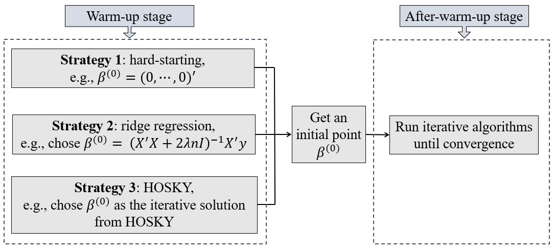
Under the above Lasso model, many iterative algorithms are proposed to minimize its objective function . Technically, these iterative algorithms are involved in two stages. The first stage is called the warm-up stage. In this stage, one decides the strategy to assign initial points. The simplest strategy is to use pre-specified vectors as initial points, say, a vector of all zeros. An alternative strategy is to use the solution from the ridge regression [3] as the initial points [4, 5]. In this paper, we propose one more option called HOSKY. The initial points generated by HOSKY, on the one hand, are more computationally efficient; on the other hand, accelerate the overall convergence rate. We skip its detailed description here and articulate its implementation later in Section 2. The second stage, which is right after the warm-up stage, is called the after-warm-up stage. In this stage, one runs a selected iterative algorithm with the initial point from the warm-up stage until convergence. The visualization of the correlation between these two stages is available in Fig. 1.
The objective of this paper is to develop a new strategy in the warm-up stage. The proposed strategy, on the one hand, is more computationally efficient than the existing strategies (see our comparison criteria in Section 1.2 and literature review in Section 1.3); one the other hand, helps to accelerate the calculation in the after-warm-up stage (see various numerical simulations in Section 4).
1.2 Criteria to Measure Computational Efficiency
In this section, we present the criteria to measure the computational efficiency in the warm-up stage, as well as the contribution of the warm-up stage to convergences.
First, we introduce the criterion to measure the computational efficiency in the warm-up stage. It is widely acknowledged that, different initial points might leads to different closeness to the optima . If one takes lots of computations to get an initial point, this initial point will tentatively converge to the optima shortly. Otherwise, if one takes limited computations to derive an initial point, one might end with slow convergence to the optima in the after-warm-up stage. To compare the computational efficiency of different warm-up strategies, we measure their total number of numerical operations to achieve a common warm-up precision . And this warm-up precision defines the closeness between and . The mathematical definition of this criterion is articulated in the following statement.
Criterion 1.1 (Criterion to measure the computational efficiency in the warm-up stage).
Suppose there are two strategies A and B in the warm-up stage. Assume both of them are iterative algorithms and give iterative solutions after iterations in the warm-up stage. We declare strategy A is more computationally efficient than B if A’s total number of numerical operations (such as plus, minus, multiplications and divisions) to achieve
| (2) |
is less than B’s total number of numerical operations to achieve Here is a pre-specified warm-up precision and commonly not set as tiny number close to 0, i.e., .
The above criterion indicates that the computational complexity is in terms of . And this correlation is usually adopted in the big notation. For example, if the computational complexity of a warm-up algorithm is , then it means that to achieve the warm-up precision, the number of numeric operations can be upper bounded by a constant multiplies . In theory, an algorithm is more computationally efficient than an algorithm. Moreover, an algorithm has an even lower order of complexity. Although the order of computational complexity gives an upper bound of the number of numerical operations to achieve the warm-up precision , it does not say anything about the average performance of the algorithm. It is possible that an algorithm with larger upper bounds performs better in some cases than an algorithm with lower upper bounds.
The aforementioned Criterion 1.1 compares two iterative algorithms in the warm-up stage. And it is not recommended to use Criterion 1.1 to compare an iterative algorithm with a closed-form strategy (like ridge regression). This is because, a closed-form strategy gives a fixed warm-up precision, which is independent of the warm-up precision : no matter how much changes, the total number of numerical operations to get the closed-form initial points is fixed. On the contrary, the iterative strategy depends on the warm-up precision : a smaller leads to a larger total number of numerical operations and vice versa.
In this paper, we call the total number of numerical operations to achieve the warm-up precision as order of computational complexity in the warm-up stage. In the remainder of this paper, we use it as our primary measure to compare different iterative algorithms. Besides, we also use running time to achieve the warm-up precision as our secondary measure in the numerical simulations in Section 4. The reason why we adopt the order of computational complexity as our primary measure is that it records the number of numerical operations (like plus and minus), which is independent of different computer platforms. While running time, though widely used, depends on different platforms. Consequently, the order of computational complexity provides a more reliable way for us to compare different algorithms.
Second, we introduce the criterion to measure the contribution of a warm-up stage to the overall convergence. Recall in Fig. 1 that, an iterative algorithm to solve Lasso can be cut into two stages: warm-up stage and after-warm-up stage. In the warm-up stage, one stops when the warm-up precision is achieved. And usually (e.g., ). In the after-warm-up stage, one stops when the after-warm-up precision is achieved. And this controls the overall convergence. Commonly we have (e.g., ).
To measure the contribution of different warm-up strategies to the overall convergence, one can use the following procedure.
-
•
Step 1: run different warm-up strategies until a common warm-up precision is achieved. This makes the initial points from different warm-up strategies share the same closeness to the optima . And the only difference lies in the number of numerical operations to arrive at .
-
•
Step 2: select an algorithm in the after-warm-up stage. The selected algorithm can minimize until convergence. Options of the algorithms in the after-warm-up stage are reviewed in Section 1.3.
-
•
Step 3: run the algorithm selected in Step 2 until a common after-warm-up precision is achieved.
-
•
Step 4: compare the total number of numerical operations (warm-up stage + after-warm-up stage).
The above procedure is summarized in the following proposition.
Criterion 1.2 (Criterion to measure the contribution of the warm-up stage to overall convergence).
Suppose there are two strategies A and B in the warm-up stage. Assume both of them are iterative algorithms and they both achieve a common warm-up precision in (2). With the initial points by strategies A and B available, one can run a selected algorithm in the after-warm-up stage, and minimize until a common after-warm-up precision is achieved. We declare strategy A contributes more to convergence than B if A’s total number of numerical operations (warm-up stage + after-warm-up-stage) is smaller than B.
As readers will see in the rest of the paper, both Criterion 1.1 and Criterion 1.2 are used in Section 3 and Section 4 to theoretically/numerically verify that the proposed HOSKY algorithm is more computationally efficient in the warm-up stage and also accelerates the convergence in the after-warm-up stage.
1.3 Literature Review
In this section, we present representative strategies in the warm-up stage, and also briefly review the representative algorithms in the after-warm-up stage.
In the warm-up stage, people can use different strategies to assign initial points. The first strategy is to set the initial points as a pre-specified vector. For example, one can set , where denotes the initial point. Then one can run a selected iterative algorithm to minimize until convergence. This strategy is adopted in many papers, like [6, 7], given its simplicity. The second strategy is to use the solution from ridge regression [3] as the initial points. Specifically, one can set as
| (3) |
This strategy is also preferred by many researchers like [4, 5] due to its closed-form propriety. To get the above closed-form solution, the major computation lies in the inverse of the matrix . As indicated by [8, 9, 10], the computational complexity to inverse a matrix is at least . In additional to solving (3) directly, one can also use the coordinate descent algorithm to get an iterative solution [11]. Since we will introduce this algorithm in the next paragraph, we skip its detailed description here. And more details can also be found in Appendix A.3.
In the after-warm-up stage, with the initial points from the warm-up stage, one can run a selected iterative algorithm until convergence. The representatives of these iterative algorithms are reviewed as follows. The first representative algorithm is the iterative shrinkage threshold algorithm (ISTA) proposed by [6]. It approximates the first term of , i.e., , by its second-order Taylor expansion. Then, they use its gradient, Hessian matrix, and soft-thresholding function to iteratively update the solution. The second representative algorithm is fast iterative shrinkage-thresholding algorithms (FISTA) proposed by [7], which is an accelerated version of ISTA. Compared with ISTA, FISTA takes advantage of the accelerated gradient descent (AGD) algorithm and uses the gradients at the previous two solutions to learn from the “history.” The third representative algorithm is the coordinate descent (CD) algorithm in [11]. Different from ISTA and FISTA, which updates their solution globally, CD utilizes the coordinate descent to update the solution. A R package named glmnet has fueled its adoption. The fourth representative algorithm is the smooth L1 algorithm (SL) in [12]. Compared with ISTA. FISTA, CD, which targets directly at the minimization of , SL aims to find a surrogate of . The surrogate function is
where . This surrogate function is twice differentiable by taking advantage of the non-negative projection operator of (seeing equations (2) and (3) in [13] for more details). Consequently, the EM algorithm [12] is used for the optimization. The fifth representative algorithm is the path-following (PF) algorithm in [14, 15, 16]. It begins with a large penalty parameter , which leads all the estimated coefficients to . Then it tries to identify a sequence of decreasing penalty parameter , such that when is between two kink points, the support set (the set of non-zero entries of estimated ) remains unchanged. Moreover, the estimated elementwisely is a linear function of . However, when one is over the kink point, the support is changed.
It is worth mentioning that, part of the algorithms in the after-warm-up stage can also be used in the warm-up stage. These algorithms are ISTA, FISTA, CD, and SL. For example, one can run 20 iterations in ISTA and input the ISTA’s solution as the initial point in the after-warm-up stage, where FISTA will run 1,000 iterations until convergences. Under this scenario, ISTA can be regarded as a warm-up strategy. In the remainder of this paper, we will not only compare HOSKY with representative warm-up strategies (like ridge regression), but we will also compare it with some after-warm-up algorithms (like ISTA, FISTA, CD, and SL) since they can be both applied in warm-up stage and after-warm-up stage.
1.4 Our Motivation and Contribution
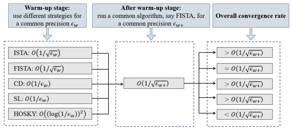
Our motivation to develop the HOSKY algorithm includes two. First, if one uses ridge regression to assign the initial point – which is frequently used – one will end up with at least numerical operations. Yet, in Lasso, usually, the number of covariates is much larger than the sample size , i.e., . So it is computationally expensive if one uses ridge regression to assign initial points. And this makes it desirable to develop a strategy with lower computational complexity. Second, if one uses a pre-specified vector like as the initial point– which is also frequently used – and runs a selected algorithm (say, FISTA) until convergence, the convergence rate is at best . This strategy, in the other words, can be regarded as using FISTA in both the warm-up stage and after-warm-up stage: in the warm-up stage, FISTA stops until is achieved; in the after-warm-up stage, FISTA stops when is achieved. Thus, the overall convergence rate is the exactly the convergence rate of FISTA, i.e., . However, if one can expedite the warm-up stage with convergence rate of , then the overall convergence is likely lower than . (See a visualization of our motivations in Fig. 2). Given the above two motivations, we develop the HOSKY algorithm, which accelerates the computation in the warm-up stage, and thus improves the overall convergence rate.
The main contribution of the proposed HOSKY algorithm is its provable lower order of computational complexity in the warm-up stage, compared with the existing algorithms introduced in Section 1.3. Specifically, to achieve a common warm-up precision in Criterion 1.1, HOSKY achieves a log-polynomial order of , while ISTA, FISTA, CD, SL have a polynomial order of (see Table 1). So, HOSKY has lower computational complexity than ISTA, FISTA, CD, and SL. For ridge regression, since it gives a closed-form solution, its computational complexity is independent of . For PF, we exclude it from the comparison, since it only works for a subset of the Lasso problem and there is no guarantee that its computational complexity is bounded. Another contribution of HOSKY is that, as reflected by various simulations in Section 4, with the speed-up on the warm-up stage, the computation in the after-warm-up stage can also be expedited. This demonstrates that our proposed HOSKY algorithm is beneficial to the final convergences, and thus indicates the importance of our work.
method1 ISTA2 FISTA3 CD4 SL5 HOSKY Order of complexity 1 Ridge regression is excluded since its complexity is not in terms of . 2,3,4,5 These methods are reviewed in Section 1.3.
The organization of the rest of the paper is articulated as follows. We develop our proposed HOSKY algorithm in Section 2. The related main theory is established in Section 3. Numerical examples are shown in Section 4. Some discussions are presented in Section 5. In A, we summarize some necessary technical details of these benchmark algorithms. A useful theorem on accelerated gradient descents is restated in B. All the technical proofs are relegated to C.
2 The Proposed Algorithm
The main idea of the HOSKY algorithm is articulated as follows. Instead of minimizing in (1) directly, we minimize a sequence of surrogate functions in a sequential manner. Specifically, we minimize first and then minimize , until we arrive at . And the length of the surrogate functions is decided by the pre-specified warm-up precision : a small is likely to lead a large value of and vice versa. A nice propriety of the sequence of the surrogate functions is that, it gets closer and closer to when , and we call it as a homotopy path. Additionally, when minimizing a given surrogate function for any , we applied the accelerated gradient descent (AGD) algorithm.
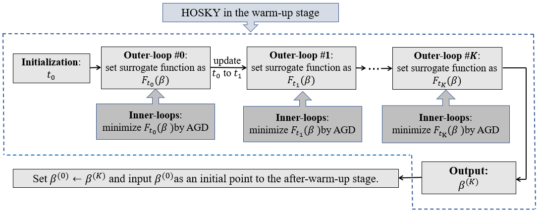
Technically, the above HOSKY algorithm involves two loops: in the outer-loop, we update to ; and in the inner-loop, we minimize by the AGD algorithm. By optimizing this sequence of surrogate functions, one can get an iterative estimator , which can be served as an initial point to minimize . The visualization of the two types of loops in HOSKY is available in Fig. 3.
To enable the above homotopy path idea, there are three technical blocks. The first block is the design of the surrogate function for any . The second block is the design of the hyper-parameters , which forms the outer-loops in HOSKY. The third block is the optimization strategies to minimize for any , which forms the inner-loops in HOSKY. In the remainder of this section, we will discuss these three blocks separately in Section 2.1, Section 2.2, and Section 2.3.
2.1 Design of Surrogate Functions
In this section, we discuss the design of the surrogate function of for a general hyper-parameter . In this paper, we design in the form of
| (4) |
where the surrogate function replaces the penalty into . Here where is the -th entry of and the function is
| (7) |
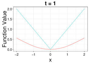
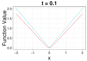
Here is a hyper-parameter controlling the closeness between and . And we will discuss the value of in Section 2.2. In Fig. 4, we display the curve of under different values of . It can be seen that, when gets smaller, become closer to the counterparts of the function .
For the above surrogate function and , they have three nice proprieties. The first nice property of is that it is quadratic near and almost linear outside. This property make the overall surrogate function both strongly convex and well conditioned. Consequently, a lower order of complexity becomes achievable when we minimize by the AGD algorithm. Specifically, one can prove a log-polynomial computational complexity for this algorithm at the warm-up stage. The second nice property of is that, if we decrease the value of , the surrogate function gets closer and closer to . This is exactly what happens in HOSKY: when the outer-loop index , we get a decreasing hyper-parameter sequence . Accordingly, the surrogate function sequence gets closer and closer to . The third nice propriety of is that, the difference between and can be bounded, as shown in Lemma 2.1.
 |
 |
 |
Lemma 2.1.
Suppose that from the beginning of our algorithm to the end of our algorithm, we have that for any and . Then for any , the surrogate function in equation (7) has the following property:
| (8) |
In the above lemma, viewing from the right-hand side of inequality (8), we find the surrogate function is always below . Besides, viewing from the left-hand side of inequality (8), we find shows that is not too below . This inequality guarantees the estimator of HOSKY is close to because their objective function is close, which can be used as initial points in the after-warm-up stage.
The motivations to design the surrogate function include two. First, we hope the surrogates are strongly convex and well-conditioned. If so, the gradient descent method (like the AGD algorithm) can achieve a very fast convergence rate. However, for the original objective function in Lasso, it is not strongly convex given the norm ( in our paper). Second, it is widely acknowledged that the quadratic function (such as ) can be easily proved to be strongly convex. Motivated by the aforementioned two facts, we try to replace by , which is quadratic near and almost linear outside. By making this replacement, the surrogates can be strongly convex. Yet, it is nontrivial to find a good surrogate function . We list the requirements of in Condition 2.2.
Condition 2.2.
Desirable conditions for function are in the following.
-
1.
When gets closer to 0, we have close to the absolute value function .
-
2.
Function has the second derivative with respective to .
-
3.
For fixed , function is quadratic on , here indicates that the left hand side (i.e., ) is the variable in the function in the right hand side (i.e., ). We follow this convention in the rest of this paper.
-
4.
Function is . Here is the set of all continuously differentiable functions.
Proof.
See C.2. ∎
We acknowledge that, the design of in equation (7) is not unique but needs to satisfy some special requirements. Generally speaking, we can assume that has the following format:
| (11) |
Then requirement in Condition 2.2 is equivalently transformed into:
-
1.
both and are .
-
2.
, , , so that .
Besides, we wish the second derivative of has the format of , where is a function of and is a constant. Accordingly, it is reasonable to suppose that . Combining all the requests above, one has
Since , we choose . Other choices of can be function or other functions, which makes as a constant when .
2.2 Design of Outer-loops
In this Section, we discuss the outer-loop of HOSKY. As indicated by Fig. 3, the objective in the -th outer-loop is to set the surrogate function as and then update the hyper-parameter from to . Since we already discuss the design of the surrogate function in Section 2.1, we will focus on the hyper-parameter in this section. Particularly, we will cover three parts: (1) the length of the hyper-parameters , (2) the initial value of the hyper-parameter , and (3) the updating rule from to for any .
Theoretically, the total number of outer-loops is decided by the pre-fixed warm-up precision , i.e.,
With the above , it is guaranteed that the difference between and is bounded by . And a small warm-up precision usually leads to a large number of outer-loops . However, in practice, one can always set as a pre-fixed positive number, say , without caring about the value of and . In this way, a larger value of tentatively leads to a smaller value of .
For the initial value of the hyper-parameter , a natural motivation is to keep it relatively small. This is because, with an unnecessarily large , one would end up with more outer-loops if one starts. Consequently, one gets more numerical operations, which leads to higher computational complexity. So a minimal value of is desired. In our proposed HOSKY algorithm, we design such minimal to ensure that when , the initial estimator is going to be bounded by entrywisely. Under this motivation, we design the minimal value of in equation (12) of Lemma 2.4.
Lemma 2.4.
Suppose in a Lasso problem, we have the response vector and a model matrix . For our proposed HOSKY algorithm, there exist a value that satisfies the following:
| (12) |
where When one chooses the aforementioned as the initial point in the proposed algorithm, one has for any , where denotes the -th entry in the vector .
Proof.
See C.1. ∎
For the updating rule from and for any , there is a closed-from correlation: Here is set to be a predetermined value. As one get , a decreasing sequence of forms, which makes the surrogate function become closer and closer to (recall Fig. 4). In practice, a small value of is preferred (say ), since we prefer can get close to gently.
2.3 Design of Inner-loops
In this section, we discuss the inner-loop in HOSKY. Recall in Fig. 3, the objective of the inner loop is to minimize by using the AGD algorithm, for any .
A key question in the inner-loop is to decide the number of AGD iterations, or the number of inner-loops. If one runs a large number of AGD iterations, the solution will be tentatively close to convergence. However, a large number of AGD iterations leads to high computational complexity. To save computation, we do not iterative the AGD algorithm until convergence, instead, we stop the AGD algorithm once a pre-specified inner-loop precision is achieved. Mathematically, in the -th outer-loop, one can stop the AGD algorithm after inner-loops, where is defined as
| (13) |
Here denotes the AGD solution in the -th inner-loop of the -th outer-loop, and we have This pre-specified inner-loop precision is set to control the convergence of the AGD algorithm is not very poor. In HOSKY, one can set it as
| (14) |
The justification of our choice of is elaborated in our proof, whose detailed derivation can be found in C.4. Please note that the above inner-loop precision is different from the warm-up precision and after-warm-up precision . Specifically, the warm-up precision decides the number of outer-loops, while the inner-loop precision decides the number of inner-loops in the -th outer-loop.
It is worth noting that, theoretically, our algorithm can achieve the order of complexity of in the warm-up stage. Yet, in practice, it may not be implementable. The matter of fact is that the stopping rule of the inner-loop requires knowing the value of , which is not possible. However, we may use some alternatives, such as stopping the inner-loop after a fixed number of inner-loops (say 100). By using this alternative, if one sets the number of inner-loops conservatively (for example, set as 200 while 100 is theoretically sufficient), then one will end with a computational complexity higher than . And this is the reason why we state the proposed HOSKY algorithm has a provable computational complexity of .
2.4 Summary of the Proposed HOSKY Algorithm
In this section, we summarize the proposed HOSKY algorithm, which has two layers of loops: the outer-loop and the inner-loop. The pseudo code to summarize the objective of these two types of loops is available in Algorithm 1, and a detailed implementation is available in Algorithm 2.
In outer-loops, we iterate the sequence of the surrogate functions defined in (4). The difference between and lies in the last item: it is in , while it is in . By iterating in outer-loops, it forms a homotopic path with getting closer and closer to as . And at the beginning of each outer-loop, it takes the stopping position from the previous outer-loop.
In inner-loops of the -th outer loop, we iteratively minimize in (4) by the AGD algorithm. Theoretically, one can save computations by stopping the AGD iterations earlier than convergence. The theoretical stopping rule is shown in (13): we only require AGD to minimize when a pre-specified AGD precision arrives. Yet in practice, this theoretical stopping rule is hard to exactly achieve given the unknown in (13). Thus, a conservative way in the inner-loop is to run a relatively large number of AGD iterations to ensure is achieved, though one might end with relatively higher computations.
The above ideas to develop HOSKY have two advantages. First, in the inner-loops, we can get a convergence rate of when minimizing by the AGD algorithm, since is differentiable and strongly convex. And this is the fastest convergence rate that can be achieved. Second, in the outer-loops, the homotopy path gets closer and closer to when . And this improved closeness helps to reduce the approximation error between to .
-
1.
: response vector;
-
2.
: model matrix;
-
3.
: the turning parameter trading-off the goodness-of-fit and the sparsity of the Lasso estimator;
-
4.
: total number of outer-loops;
-
5.
: total number of inner-loops at the -th outer loops .
-
1.
: response vector;
-
2.
: model matrix;
-
3.
: the turning parameter trading-off the goodness-of-fit and the sparsity of the Lasso estimator;
-
4.
: total number of outer-loops;
-
5.
: total number of inner-loops at the -th outer loops .
3 Order of Complexity of the HOSKY Algorithm
This section discusses the order of computational complexity of the proposed HOSKY algorithm. Recall that the order of computational complexity is defined as the number of numerical operations needed to achieve the warm-up precision in (2), and always comes in a big notation. Because our proposed HOSKY algorithm involves two layers of loops, the order of computational complexity is in the order of the product of (i) the number of inner-loops, (ii) the number of numerical operations in each inner-loop, (iii) the number of outer-loops. In the remainder of this section, we will discuss (i), (ii), and (iii), respectively.
First, the number of inner-loops can be found in Lemma 3.1.
Lemma 3.1 (Number of inner-loops).
Recall that a Lasso problem has a response vector and a model matrix . To minimize the Lasso objective function our proposed HOSKY algorithm minimizes in the -th outer-loop by the AGD algorithms. Instead of converging to the minimizer of , we apply an early stopping rule (13) with set as in (14). It is guaranteed that, under the condition of Lemma 2.1, one can achieve the inter-loop precision in (13) after inner-loops, where is a constant that does not depend on the value of .
Proof.
See C.3. ∎
Second, we notice the number of numerical operations in one inner-loop is of order . This is because the computation is dominated by the matrix multiplication of as shown in Line 2 in Algorithm 2.
Finally, the minimal number of outer-loops is summarized in Lemma 3.2.
Lemma 3.2 (Number of outer-loops).
Proof.
See C.4. ∎
With all the above blocks, we develop the main theory, i.e., the order of computational complexity to achieve the warm-up precision of our proposed HOSKY algorithm.
Theorem 3.3 (Main theory).
Proof.
See C.5. ∎
4 Numerical Examples
In this section, we compare the performance of HOSKY with three benchmarks through various numerical experiments. The selected three benchmarks are ridge regression, ISTA, and FISTA (reviewed in Section 1.3). Here we exclude CD and SL since they share the same order of computational complexity as ISTA. Additionally, we exclude PF given its possible unbounded computational complexity and its restriction for applications to general cases.
In this section, three numerical examples are shown. The first example handles image de-noising. Through this example, we will see the proposed HOSKY algorithm can deblur a noised image. Although the deblurred image is not completely clear – since HOSKY focuses on the warm-up stage with warm-up precision – but it serves as a good initial point for people to discriminate the major characters in the images at first glance. The second example compares the computational complexity of HOSKY with its benchmarks in the warm-up stage. In this example, we use sparse linear regression for illustration purposes. The third example investigates whether a good warm-up strategy expedites the convergences. And this example can be regarded as a sequel to the second example.
The selection of the tuning parameters is articulated as follows. In both ISTA and FISTA, we set the Lipschitz continuous gradient as the maximal eigenvalue of the matrix (see detailed implementation in Algorithm 3, 4). Additionally, in FISTA, we set and for any (see detailed implementation in Algorithm 4). In ridge regression, we calculate its closed-form solution as shown in (3), so there is no need to select turning parameters. In HOSKY, we select the turning parameters following Algorithm 2. Specifically, in -th outer iteration, we set the Lipschitz continuous gradient as the maximal eigenvalue of the Hessian matrix of . And the strongly convexity is set as the minimal eigenvalue of the Hessian matrix of . With both and available, we set and to be used in the inner-iterations. Note that users are welcome to calculate the above turning parameters by the line search method [18].
4.1 Simulation 1: Image De-nosing
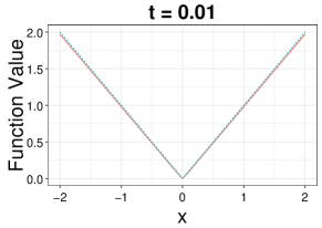
In this simulation, we compare our proposed HOSKY algorithm with ridge regression, ISTA, and FISTA in the application of image de-noising. The example image we investigated is a batman image. The image goes through a Gaussian blur of size and standard deviation followed by an additive zero-mean white Gaussian noise with standard deviation . The original and observed images are given in Fig. 5 (a) and (b), respectively.
For these experiments, we assume reflexive (Neumann) boundary conditions. We then test ridge regression, ISTA, FISTA, and HOSKY for solving problem (1), where represents the vectorized observed image, and with as the matrix representing the blur operator and as the inverse of a three-stage Haar wavelet transform. The regularization parameter is selected to be .
The de-noising results are summarized in Figure 5(c)-(f), where one can easily find that the image produced by HOSKY is of better quality than those created by its benchmarks. Besides, the computational complexity of HOSKY is lower than its benchmarks, as shown in Table 2. Though it is not exactly lower than FISTA, they are on the same scale. And the small difference might be caused by the hidden constant in the big notation.
 |
method ridge regression1 ISTA2 FISTA3 HOSKY Number of Numerical Operations 26,314,540 2,098,802 663,601 867,357 1,2,3 Ridge regression, ISTA, FISTA are introduced in Section 1.3.
4.2 Simulation 2: Compare Computational Complexity in the Warm-up Stage
In this section, we compare HOSKY with ridge regression, ISTA, FISTA under the scenario to estimate true parameters in the sparse linear regression models. The data generation mechanism is described as follows, which follows [11]. First, we generate Gaussian data with observations and covariates, with each predictor is associated with a random vector , and the model matrix is . Here we assume that the random vector follows the multivariate normal distribution with zero mean, variances being equal to , and identical population correlation , that is, the covariance matrix of has 1 on its diagonal and for its reminder entries. In this simulation, we set . The response values were generated by
| (15) |
For the value of , we discuss two scenarios:
-
•
Scenario 1: ;
-
•
Scenario 2: , where is the identity function, i.e., if , and otherwise.
Both scenarios are constructed to have alternating signs and to be exponentially decreasing. And the difference between these two scenarios lies in the sparsity in the second scenario, i.e., its when . This parameter setting assumes that most of the entries in are zero, which renders a case with sparse truth. Besides, is the white noise with satisfying the standard normal distribution . The quantity is chosen so that the signal-to-noise ratio is . The turning parameter is set to be . And in our simulation, we investigate two sets of values, i.e., and .
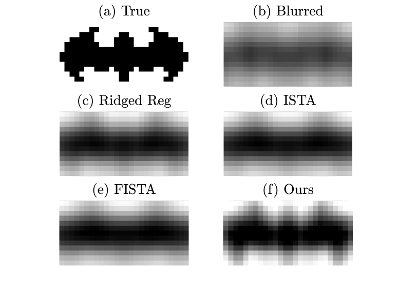
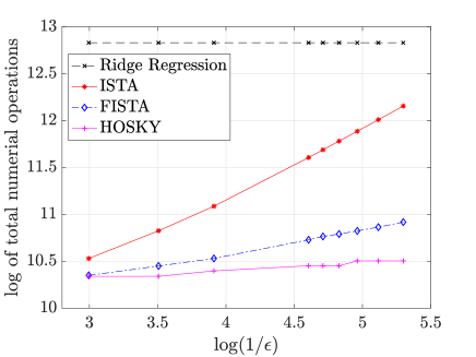
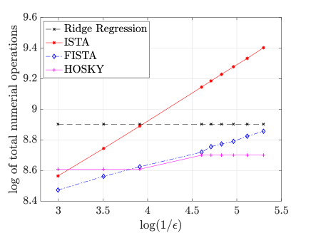
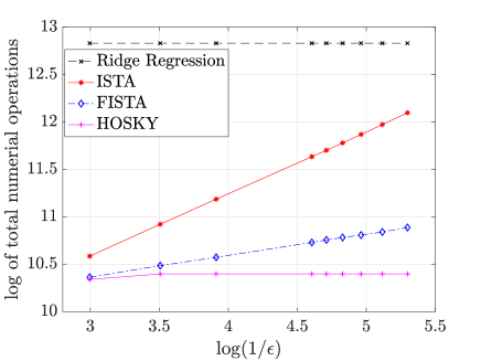
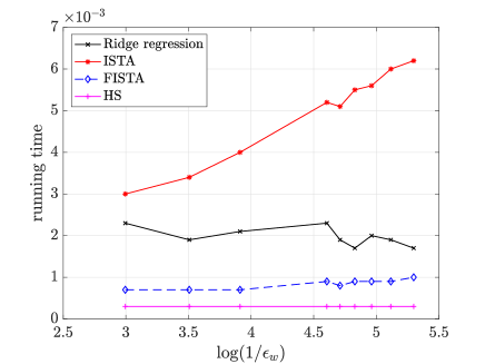
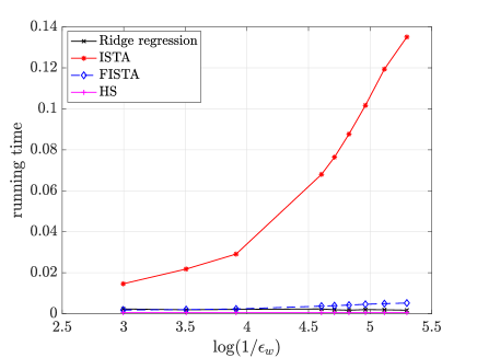
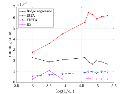
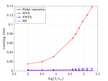
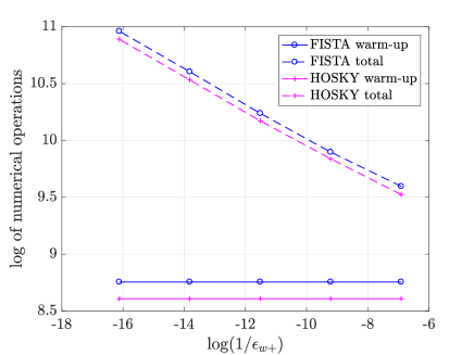
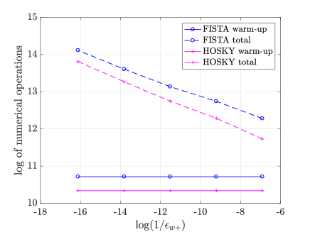
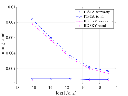
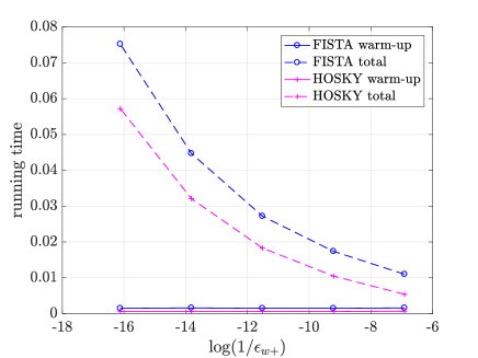
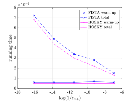
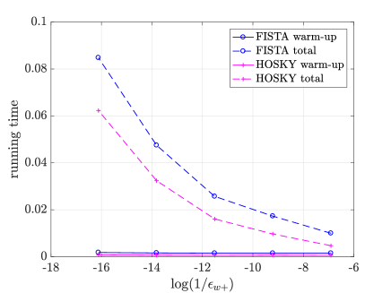
The simulation results are summarized in Table 3, Table 4 and visualized in Fig. 6, Fig. 7. We report the total number of numerical operations to achieve different values of the warm-up precision in Table 3 and Fig. 6, which is independent of the computation platform. Additionally, we report the running time in Table 4 and Fig. 7, which is based on a Macbook pro with 2.3 GHz Intel Core i5. In both Table 3 and 4, the values in cells are the number of operations/running time to achieve the different warm-up precision . In both Fig. 6, 7, the dark, red, blue, and pink lines represent the number of numerical operations/running time of ridge regression, ISTA, FISTA, and HOSKY, respectively. The x-axis is the and the y-axis is the logarithms of the number of numerical operations/ running time to achieve the corresponding warm-up precision .
From Table 3, 4 and Fig. 6, 7, we find there are some common properties shared among different methods. For example, iterative algorithms – like ISTA, FISTA, and HOSKY – take more numerical operations/running time to achieve a smaller value of . While for closed-form methods like ridge regression, its numbers of numerical operations are independent of .
From Table 3, 4 and Fig. 6, 7, we also find differences among different methods. Generally speaking, HOSKY has fewer numerical operations or less running time than its benchmarks. For example, under the first scenario with , HOSKY only requires operations. However, ridge regression, ISTA, and FISTA need , , and operations, respectively. And we also notice that when with large , the number of numerical operations of ISTA, FISTA, and HOSKY are very similar. This is because when is large, the hidden constant before the complexity ( for ISTA, for FISTA, and for HOSKY) are dominated.
Precision method Scenario 1 Ridge Regression ISTA FISTA HOSKY Scenario 1 Ridge Regression ISTA FISTA HOSKY Scenario 2: Ridge Regression ISTA FISTA HOSKY Scenario 2: Ridge Regression ISTA FISTA HOSKY 1 There is the parameters settings of our HOSKY algorithm: .
Precision method Scenario 1 Ridged Regression ISTA FISTA HOSKY Scenario 1 Ridged Regression ISTA FISTA HOSKY Scenario 2: Ridged Regression ISTA FISTA HOSKY Scenario 2: Ridged Regression ISTA FISTA HOSKY 1 There is the parameters settings of our HOSKY algorithm: . 2 The running time is based on a Macbook pro with 2.3 GHz Intel Core i5.
 |
 |
| (a) Scenario 1 () | (b) Scenario 1 () |
 |
 |
| (c) Scenario 2 () | (d) Scenario 2 () |
 |
 |
| (a) Scenario 1 () | (b) Scenario 1 () |
 |
 |
| (c) Scenario 2 () | (d) Scenario 2 () |
4.3 Simulation 3: Investigate if Good Warm-up Stages Expedite after-warm-up Stages
In this section, we investigate the contribution of the warm-up stage to convergence (the after-warm-up stage). Specifically, we will verify that the initial point assigned by HOSKY expedites the convergence in the after-warm-up stage. As indicated by both Simulation 1 and Simulation 2, among the benchmarks of HOSKY, FISTA performs the best. So in this section, we will use FISTA as a representative benchmark.
The simulation setting is the same as that we have in Section 4.2, and the comparison criterion follows Criterion 1.2. In the warm-up stage, we fix the warm-up precision as for both FISTA and HOSKY. In the after-warm-up stage, we run FISTA until the after-warm-up precision is achieved. For both the warm-up stage and after-warm-up stage, we will calculate the number of numerical operations, as well as the running time. To evaluate whether HOSKY expedites the after-warm-up stage, one can check the total number of numerical operations (warm-up + after-warm-up) to achieve the common after-warm-up precision . In addition to the total number of numerical operations, one can also compare the total running time.
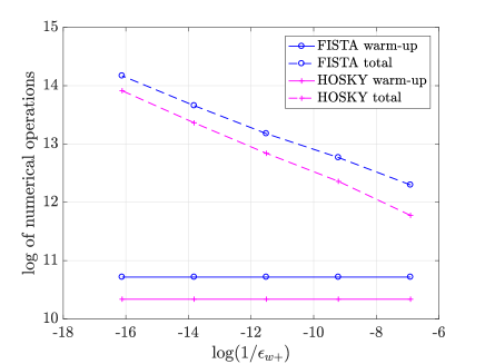
The simulation results are summarized in Table 5, Table 6 and visualized in Fig. 8, Fig. 9. We report the number of numerical operations in Table 5 and Fig. 8, which is independent of the platforms. Additionally, we report the running time in Table 6 and Fig. 9, which is based on a Macbook pro with 2.3 GHz Intel Core i5.
From the aforementioned two tables and two plots, one can draw two conclusions. First, to achieve the common warm-up precision , HOSKY requires less number of operations (or running time), compared with FISTA. To verify this conclusion, one can take a close look at Fig. 8 and Fig. 9. In these two plots, the pink solid line (HOSKY in the warm-up stage) is always below the blue solid line (FISTA in the warm-up stage). This conclusion is consistent with the conclusion we have in Section 4.2. Second, the initial points from HOSKY can expedite the calculation in the after-warm-up stage. For example, to achieve the common after-warm-up precision , if one uses the initial point from HOSKY, one only needs numerical operations (0.0006 seconds), while FISTA needs numerical operations (0.0015 seconds) in Scenario 1. The same conclusion can also be drawn from Fig. 8 and Fig. 9. In these two plots, the pink dash line (HOSKY in the after-warm-up stage) is always below the blue dash line (FISTA in the after-warm-up stage), for both the number of numerical operations and running time.
After-warm-up precision Method Stage Scenario 1 FISTA Warm-up After-warm-up Total % of warm-up HOSKY Warm-up After-warm-up Total % of warm-up Scenario 1 FISTA Warm-up After-warm-up Total % of warm-up HOSKY Warm-up After-warm-up Total % of warm-up Scenario 2 FISTA Warm-up After-warm-up Total % of warm-up HOSKY Warm-up After-warm-up Total % of warm-up Scenario 2 FISTA Warm-up After-warm-up Total % of warm-up HOSKY Warm-up After-warm-up Total % of warm-up 1 There is the parameters settings of our HOSKY algorithm: .
After-warm-up precision Method Stage Scenario 1 FISTA Warm-up After-warm-up Total % of warm-up HOSKY Warm-up After-warm-up Total % of warm-up Scenario 1 Pre-assigned value Warm-up After-warm-up Total % of warm-up HOSKY Warm-up After-warm-up Total % of warm-up Scenario 2 FISTA Warm-up After-warm-up Total % of warm-up HOSKY Warm-up After-warm-up Total % of warm-up Scenario 2 FISTA Warm-up After-warm-up Total % of warm-up HOSKY Warm-up After-warm-up Total % of warm-up 1 There is the parameters settings of our HOSKY algorithm: . 2 The running time is based on a Macbook pro with 2.3 GHz Intel Core i5.
 |
 |
| (a) Scenario 1 () | (b) Scenario 1 () |
 |
 |
| (c) Scenario 2 () | (d) Scenario 2 () |
 |
 |
| (a) Scenario 1 () | (b) Scenario 1 () |
 |
 |
| (c) Scenario 2 () | (d) Scenario 2 () |
5 Discussion
In our theoretical result, we required the presence of a constant , such that for all . Such a condition prevents the hyper-parameter from converging to zero. It will be interesting to study whether there is a way to relax this condition. In Section 5.1, we show that when the is chosen to be small enough, an early-stopped homotopic approach will find the support of the global solution, therefore, one can simply run the ordinary regression on this support set, without losing anything. In Section 5.2, we discuss other seemingly similar homotopic ideas and articulate the differences between theirs and the work that is presented in this paper.
5.1 Support Recovery and the Need for Hyper-parameter to Converge to Zero
In Theorem 3.1, we assume that there is a constant , such that for all . Such a condition prevents the hyper-parameter from converging to zero. Therefore, our result just applies to the warm-up stage of a homotopic approach to solving the Lasso problem. In this subsection, we show that under some standard conditions that have appeared in the literature, as long as we set to be small enough, the associated algorithm will find a solution with both small “prediction error” and small “estimation error.” The mathematical meaning of “prediction error” is
where for a general and defined in (7), and . And the mathematical meaning of “estimation error” in our paper is
In the remaining of this section, we will give two propositions, where we develop the conditions the a small prediction error and estimation error hold.
We begin with the prediction error, i.e., . In Proposition 5.1, we declare that there are no additional conditions needed to guarantee the small prediction error. That is, as long as we converge , our proposed algorithm can guarantee the prediction error goes to zero as well.
Proposition 5.1.
For our proposed algorithm, when , we have the perdition error where for a general and defined in (7). And .
Proof.
See C.6. ∎
After developing the prediction error, we now discuss the estimation error. A nice property of Lasso is that, it can potentially achieve the sparse estimation when , i.e., most of the entries in the Lasso estimator are zero, and only a few of them are non-zero. The index set of these non-zero entries are called support set, i.e., To show how Lasso can realize the sparse estimation, we take as an illustration example, where is the identity matrix. (More complicated model matrix can also be used, but here we use to create an example.) Then we have the linear regression model as
where is the response vector, and is the white noise. The Lasso estimator of the above linear regression model is It can be verified that
is the solution of the Lasso problem. Note that is sparse if has many components with small magnitudes. However, if we consider , instead of the penalty , we have
We can show that if and only if . This shows that is not guaranteed to be sparse.
Although is not sparse, we can still verify that has very small estimation error under some specific assumptions of the model matrix .
Proposition 5.2.
Suppose the model matrix in the Lasso problem has the following three properties:
-
1.
can be bounded by a constant, where with And is the Frobenius norm defined as , where is the th entry in matrix .
-
2.
can be bounded by a constant, where is the complement set of . And is the pseudo-inverse of matrix . The mathematical meaning of pseudo-inverse is that, suppose , which is the singular value decomposition (SVD) of . Then For the rectangular diagonal matrix , we get by taking the reciprocal of each non-zero element on the diagonal, leaving the zeros in place, and then transposing the matrix.
-
3.
, where returns the maximal absolute diagonal values of matrix , and returns the minimal absolute diagonal values of matrix . Matrix is the diagonal matrix in the SVD of matrix i.e., Matrix is the diagonal matrix of the SVD of the matrix i.e., .
Then we have when .
Proof.
See C.7. ∎
We notice that the above proposition requires a strong condition on the model matrix to achieve the support recovery. Releasing the conditions in the above proposition is an interesting future research topic.
5.2 Other Related Homotopic Ideas
It is worth noting that, in recent research, some researchers also realize the log-polynomial order of complexity (seeing [19, 20, 21, 22, 23]) in a framework similar to Lasso-algorithms. However, we would like to clarify that, there are some essential differences between our paper and these papers. First, the problem formulation in these papers is different from ours. The problem formulation these papers solve is that, they start at some initial objective problem, which is a Lasso-type objective function:
| (16) |
and then they gradually decrease the large until the target regularization is reached. When the is reached, the algorithm is stopped. However, this algorithmic solution is not optimal in (16). In other words, the solution of these papers is not exactly the Lasso solution. While in our paper, our objective function stays the same as (1) from the beginning to the end of our algorithm. Therefore, the solution we iteratively calculated is the minimizer of the Lasso problem in (1). In addition to the difference in the objective function, the assumptions between our algorithm and these papers are also different. Specifically, these papers require more additional assumptions than ours, such as the restricted isometry property (RIP), which is used to ensure that all solution path is sparse. Finally, through both our paper and these papers are called the “homotopic” method, the definition of the “homotopic” is different. Specifically, these papers use the homotopic path in the penalty parameter : they start from a very large and then shrinkage to the target . This type of method is also called “path following” in other papers, such as [15], [24], [25] and etc, instead of “homotopic path”. However, our paper uses the homotopic path in the penalty : we replace the regularization term with a surrogate function, and then by adjusting the parameters in the surrogates, to get the surrogate approximates more close to the original regularization term.
Acknowledgement
This project is partially supported by the Transdisciplinary Research Institute for Advancing Data Science (TRIAD), http://triad.gatech.edu, which is a part of the TRIPODS program at NSF and locates at Georgia Tech, enabled by the NSF grant CCF-1740776. The authors are also partially sponsored by NSF grants 1613152 and 2015363.
References
- [1] F. Santosa, W. W. Symes, Linear inversion of band-limited reflection seismograms, SIAM Journal on Scientific and Statistical Computing 7 (4) (1986) 1307–1330.
- [2] R. Tibshirani, Regression shrinkage and selection via the lasso, Journal of the Royal Statistical Society. Series B (Methodological) (1996) 267–288.
- [3] A. E. Hoerl, R. W. Kennard, Ridge regression: Biased estimation for nonorthogonal problems, Technometrics 12 (1) (1970) 55–67.
- [4] L. Melkumova, S. Y. Shatskikh, Comparing ridge and lasso estimators for data analysis, Procedia engineering 201 (2017) 746–755.
- [5] X. Sun, The Lasso and its implementation for neural networks., University of Toronto, 2000.
- [6] I. Daubechies, M. Defrise, C. De Mol, An iterative thresholding algorithm for linear inverse problems with a sparsity constraint, Communications on Pure and Applied Mathematics: A Journal Issued by the Courant Institute of Mathematical Sciences 57 (11) (2004) 1413–1457.
- [7] A. Beck, M. Teboulle, A fast iterative shrinkage-thresholding algorithm for linear inverse problems, SIAM journal on imaging sciences 2 (1) (2009) 183–202.
- [8] A. Tveit, On the complexity of matrix inversion, Mathematical Note (2003) 1.
- [9] Y. Zhao, X. Huo, A survey of numerical algorithms that can solve the lasso problems, Wiley Interdisciplinary Reviews: Computational Statistics (2022) e1602.
- [10] Y. Zhao, New progress in hot-spots detection, partial-differential-equation-based model identification and statistical computation, Ph.D. thesis, Georgia Institute of Technology (2021).
- [11] J. Friedman, T. Hastie, R. Tibshirani, Regularization paths for generalized linear models via coordinate descent, Journal of statistical software 33 (1) (2010) 1.
- [12] M. A. Figueiredo, Adaptive sparseness for supervised learning, IEEE transactions on pattern analysis and machine intelligence 25 (9) (2003) 1150–1159.
- [13] M. Schmidt, G. Fung, R. Rosales, Fast optimization methods for l1 regularization: A comparative study and two new approaches, in: European Conference on Machine Learning, Springer, 2007, pp. 286–297.
- [14] R. J. Tibshirani, J. Taylor, et al., The solution path of the generalized Lasso, The Annals of Statistics 39 (3) (2011) 1335–1371.
- [15] S. Rosset, J. Zhu, Piecewise linear regularized solution paths, The Annals of Statistics (2007) 1012–1030.
- [16] M. Y. Park, T. Hastie, L1-regularization path algorithm for generalized linear models, Journal of the Royal Statistical Society: Series B (Statistical Methodology) 69 (4) (2007) 659–677.
- [17] S. Bubeck, M. B. Cohen, Y. T. Lee, Y. Li, An homotopy method for regression provably beyond self-concordance and in input-sparsity time, in: Proceedings of the 50th Annual ACM SIGACT Symposium on Theory of Computing, ACM, 2018, pp. 1130–1137.
- [18] G. Lan, Lectures on optimization. methods for machine learning, H. Milton Stewart School of Industrial and Systems Engineering, Georgia Institute of Technology, Atlanta, GA.
- [19] L. Xiao, T. Zhang, A proximal-gradient homotopy method for the sparse least-squares problem, SIAM Journal on Optimization 23 (2) (2013) 1062–1091.
- [20] Q. Lin, L. Xiao, An adaptive accelerated proximal gradient method and its homotopy continuation for sparse optimization, in: International Conference on Machine Learning, 2014, pp. 73–81.
- [21] Z. Wang, H. Liu, T. Zhang, Optimal computational and statistical rates of convergence for sparse nonconvex learning problems, Annals of statistics 42 (6) (2014) 2164.
- [22] T. Zhao, H. Liu, T. Zhang, et al., Pathwise coordinate optimization for sparse learning: Algorithm and theory, The Annals of Statistics 46 (1) (2018) 180–218.
- [23] H. Pang, H. Liu, R. J. Vanderbei, T. Zhao, Parametric simplex method for sparse learning, in: Advances in Neural Information Processing Systems, 2017, pp. 188–197.
- [24] G. I. Allen, Automatic feature selection via weighted kernels and regularization, Journal of Computational and Graphical Statistics 22 (2) (2013) 284–299.
- [25] G. I. Allen, C. Peterson, M. Vannucci, M. Maletić-Savatić, Regularized partial least squares with an application to NMR spectroscopy, Statistical Analysis and Data Mining: The ASA Data Science Journal 6 (4) (2013) 302–314.
- [26] S. Mukherjee, C. S. Seelamantula, Convergence rate analysis of smoothed Lasso, in: Communication (NCC), 2016 Twenty Second National Conference on, IEEE, 2016, pp. 1–6.
- [27] S. Boyd, L. Vandenberghe, Numerical linear algebra background, 2010. http://www, seas. ucla. edu/-vandenbe/ee236b/lectures/num-lin-alg. pdf.
- [28] A. Beck, L. Tetruashvili, On the convergence of block coordinate descent type methods, SIAM journal on Optimization 23 (4) (2013) 2037–2060.
SUPPLEMENTARY MATERIAL
Appendix A Review of some State-of-the-art Algorithms
In this section, we will show the algorithm mechanism of these four representative we select, namely ISTA [6] in Section A.1, FISTA [7] in Section A.2, CD [11] in Section A.3, and SL [26] in Section A.4. For each algorithm, we show (i) their number of operations in a loop, (ii) the number of loops to meet the -precision in equation (2), (iii) and their according order of complexity.
A.1 Iterative Shrinkage-Thresholding Algorithms (ISTA)
ISTA aims at the minimization of a summation of two functions, , where the first function is continuous convex and the other function is smooth convex with a Lipschitz continuous gradient. Recall the definition of Lipschitz continuous gradient as follows:
If we let and with the Lipschitz continuous gradient taking the largest eigenvalue of matrix , noted as , then Lasso is a special case of ISTA.
The key point of ISTA lies in the updating rule from to , i.e., . It is realized by updating through the quadratic approximation function of at value :
| (17) |
Simple algebra shows that (ignoring constant terms in ), minimization of equation (17) is equivalent to the minimization problem in the following equation:
| (18) |
where the soft-thresholding function in equation (22) can be used to solve the problem in equation (18):
| (22) |
The summary of ISTA algorithm is presented in Algorithm 3.
It can be seen from line 4 in Algorithm 3 that the number of operations in one loop of ISTA is . This is because that the main computation of each loop in ISTA is the matrix multiplication in . Note that the matrix can be pre-calculated and saved, therefore, the order of computational complexity is [27].
In addition to the operations in each loop, we also develop the convergence analysis of ISTA in the following equation [7, Theorem 3.1]. To make it more clear, we list [7, Theorem 3.1] below with several changes of notation. The notations are changed to be consistent with the terminology that are used in this paper.
Therefore, to achieve the -precision, i.e., , at least loops are required, which leads to the order of complexity .
A.2 Fast Iterative Shrinkage-Thresholding Algorithms (FISTA)
Motivated by ISTA, [7] developed another algorithm called Fast Iterative Shrinkage-Thresholding Algorithms (FISTA). The main difference of ISTA and FISTA is that FISTA employs an auxiliary variable to update from to in the second-order Taylor expansion step (i.e., the one in equation (17)); More specifically, they have
| (24) |
where is a specific linear combination of the previous two estimator , in particular, we have . FISTA falls in the framework of Accelerate Gradient Descent(AGD), as it takes additional past information to utilize an extra gradient step via the auxiliary sequence , which is constructed by adding a “momentum” term that incorporates the effect of second-order changes. For completeness, the FISTA is shown in Algorithm 4.
Obviously, the main computational effort in both ISTA and FISTA remains the same, namely, in the soft-thresholding operation of line 4 in Algorithm 3 and 4. The number of operations in each loop of FISTA is still . Although for both ISTA and FISTA, they have the same number of operation in one loop, FISTA has improved convergence rate than ISTA, which is shown in the following theorem [7, Theorem 4.4].
Theorem A.2.
Consequently, FISTA has a faster convergence rate than ISTA, which improves from to . This is because that, to update from to , ISTA only considers , however, FISTA takes both and into account. To achieve the precision , at least loops are required, which leads to an order of complexity of .
A.3 Coordinate Descent (CD)
The updating rule in both ISTA and FISTA involve all coordinates simultaneously. In contrast, [11] proposed a Lasso-algorithm that cyclically chooses one coordinate at a time and performs a simple analytical update. Such an approach is called coordinate gradient descent.
The updating rule (from to ) in CD is that, it optimizes with respect to only the th entry of where the gradient at in the following equation is used for the updating process:
| (26) |
where is a vector of length , whose entries are all zero expect that the th entry is equal to . Imposing the gradient in equation (26) to be , we can solve for as follows:
where is the soft-thresholding function defined in equation (22). This algorithm has been implemented into the a R package, glmnet, and we summarize it in Algorithm 5.
After reviewing the algorithm of CD, we develop the order of complexity of CD. Firstly, the number of operations in each loop of CD is . It can be explained by the following two reasons. (i) While updating (line 5 in Algorithm 5), it costs operations because of . (ii) From line 4 in Algorithm 5, we can see that all entries of are updated one by one. Combining (i) and (ii), we can see that the number of operations need in one loop of CD is of the order .
The convergence rate of CD is derived as a corollary in [28, Corollary 3.8] and here we list the corollary as a theorem below. We changed several notations to adopt the terminology in this paper:
The above equation shows that, to achieve the precision -precision, at least
loops are required, which leads to an order of complexity of
As suggested by our reviewers, it is worth noting that CD is a generic algorithm, where both Lasso and ridge regression are two applications. So we also list its application in ridge regression below and its computational complexity is similar to the conclusion in Theorem A.3.
-
1.
The response vector with its -th entry denoted as ;
-
2.
The model matrix with its -th entry denoted as ;
-
3.
The penalty parameter ;
-
4.
The total number of iterations ;
-
5.
The soft -thresholding function
A.4 Smooth Lasso (SL)
The aforementioned Lasso-algorithms all aim exactly at minimizing the function . On the contrary, [26] used an approximate objective function to solve the Lasso. Their method is called a Smooth-Lasso (SL) algorithm. The main idea of SL is that it use a smooth function—— to approximate the penalty, and Accelerated Gradient Descent (AGD) algorithm is applied after the replacement. Therefore, the objective function of SL becomes . The pseudo code of SL is displayed in Algorithm 7.
For the computational effort, it mainly lies in the calculation of , where the is a vector of length , whose th entry is . Accordingly, the main computational effort of each loop of SL is the matrix multiplication in , which cost operations. On the other side, proved by [26], the approximation error of in SL is shown in equation (28).
So to achieve the -precision, SL needs , which results in the order of complexity .
A.5 Path Following Lasso-Algorithm
As mentioned in Section 1, the path following Lasso-algorithm has two drawbacks. First, it is not guaranteed to work in general cases. Second, there is no theoretical guarantee that the order of complexity of a path following Lasso-algorithm is low, considering that the maximum number of loops can be as large as , where is the number of predictors. In this section, we provide mathematical details to support the above two drawbacks. The structure of this section is described as follows. In Section A.5.1, we provide a counter example that the path following Lasso-algorithm is not workable, which represents a general category of design matrix and coefficient . In Section A.5.2, we provide mathematical details to support the second drawback of the path following Lasso-algorithm.
A.5.1 Details to Support the first Drawback of Path Following Lasso Algorithm
In this section, we provide a counter example that the path following Lasso-algorithm is not workable. This counter example represents a general category of design matrix and coefficient . We use the following counterexample to argue that a path following approach does not work in the most general setting.
Before representing the concrete counter example, let us discuss the key step in designing a path following Lasso-algorithm. For a general solution derived by path following Lasso-algorithm, i.e., , it is the minimizer of (1), so it must satisfy the first order condition of (1):
| (29) |
where and is a vector, whose th component is the sign function of :
If we divide the indices of into and its complements , then we can rewrite equation (29) as
where is the subvector of only contains elements whose indices are in and is the complement of . Besides, is the subset of , only contains the elements whose indices are in , and is the complement to . Matrix is the columns of whose indices are in , and is the complement of .
Suppose we are interested in parameter estimated under and , i.e., . Then must satisfy the following two system of equations:
| (30) |
| (31) |
From the above two system of equations, we have the following:
| (32) |
That is, if one decrease to , one must strictly follow (32).
Following the above key step in the path following Lasso-algorithm, we represent a counter example as follows. Suppose . The model matrix , where is the first two columns from a orthogonal matrix , and for , we have with . The response vector is generated by
If are very large number, say, 200, 100, and is not that large, say, 1. Then the following algorithm works as follows:
-
•
Loop 0: We start with , then we know that and .
-
•
Loop 1: When changes from to , from (29), we know that .
-
•
Loop 2: Similar to the first loop, when decrease to , we have .
-
•
Loop 3: This is where problem happens. From (32), we know that , we have
Since and , we have the right hand side of the above equation as a all-one vector, i.e, . To make the left hand side equals to , we can only take , which gives us .
However, from the data generalization, we know that the true support set is . Therefore, one will not be able to develop a path following algorithm to realize correct support set recovery. At least not in the sense of inserting one at a time to the support set. In the above example, since a path following approach can only visit three possible subsets, it won’t solve the Lasso problem in general.
A.5.2 Details to Support the Second Drawback of Path Following Lasso-Algorithm
In this section, we provide more technical details to support the second drawback of path following Lasso-Algorithm. Recall the main idea of path following Lasso-Algorithm is that, it begins with a large , which makes the estimated , and accordingly its support set (empty set). Then it tries to identify a sequence of the penalty parameter as follows:
such that for any , when we have the support of (which is a function of ) i.e., , remains unchanged. Moreover, within the interval , vector elementwisely is a linear function of . However, when one is over the kink point, the support is changed/enlarged, i.e., we have or even .
A point deserves attention is that, if , the total number of kink points is small, then the path following algorithm is efficient, i.e., it only requires numerical operations. In particular, if the size of supports are strictly increasing, i.e., we have
then we have , and accordingly the computational complexity can be bounded by . However, it turns out bounding the value of is an open question. In recent papers such as [14, 15], we can see that bounding is an open problem.
Appendix B An Important Theorem
Our proof will rely on a result on the number of steps in achieving certain accuracy in using the accelerate gradient descent (AGD) when the objective function is strongly convex. The result is the Theorem 3.7 in [18]. We represent the theorem here for readers’ convenience. We introduce some notations first. Suppose ones wants to minimize a convex function in a feasible closed convex set . We further assume that is a differentiable convex function with Lipschitz continuous gradients , i.e., , we have
where represents the gradient of function . Furthermore, we assume that is a strongly convex function, i.e., , there exist , such that we have
This type of function is called the -smooth and -strongly convex function. Recall that our objective is to solve the following problem:
In the following, we present one version of the accelerated gradient descent (AGD) algorithm. Given for , we set
| (33) | |||||
| (34) | |||||
| (35) |
for some , and . And here is the prox-function (or Bregman’s distance), i.e.,
with . By applying AGD as shown in (33)-(35), the following theorem presents an inequality that can be utilized to determine the number of loops when certain precision of a solution is given.
Theorem B.1.
Appendix C Proofs
C.1 Proof of a Lemma
The proof of Lemma 2.4 is as follows.
Proof.
In this proof, we will do two parts.
First, we will prove the existence of the initial point stated in (12). We know that
The above indicates that when is very large, the defined in (12) will exist.
Next, we will verify that, if is chosen as shown in (12), i.e,
we have . It can be verified that,
| (37) |
where is a special case of when is large enough to include all the coefficient into the interval . Utilizing the above fact that the minimizer in (37) when satisfies the condition that its coordinates are within , we have
Thus, if we choose as shown in (12), i.e.,
we can verify that , , i.e., . ∎
C.2 Proof of a Lemma
The Proof of Lemma 2.1 is as follows.
Proof.
Because is a even function, we only consider the positive in the remaining of the proof.
First, when , one has
which is a quadratic function with the axis of symmetry, being larger than . Therefore, one has
Then we discuss the scenario when , where
which is a decreasing function of variable . Therefore,
where we further have .
By the combination of two scenario ( and ), we prove the statement in equation (8). ∎
C.3 Proof of a Theorem
The proof of Theorem 3.1 can be found below.
Proof.
To begin with, we revisit some notations in linear algebra. For matrix , we use to indicate the th entry in matrix . Besides, its maximal/minimal eigenvalue is , respectively.
It is known that, the condition number of function is defined by the ratio between the maximal and minimal eigenvalue of its Hessian. Recall that, the th entry of the Hessian matrix of the surrogate function , noted as , is
Note that the Hessian matrix is diagonal and positive definite; therefore one can easily find its minimum and maximum eigenvalues. So the condition number of function , noted as , is
| (39) | |||||
| (42) |
Equation (39) is due to the definition of the condition number. Inequality (C.3) is because of the two fact. First, for the maximal eigenvalue of summation of two matrix , i.e., , is no more than summation of maximal eigenvalue separately, . Second, similar to the maximal eigenvalue, the minimal eigenvalue follows the similar rule that . The equality in (C.3) is due to the fact that matrix is diagonal with positive diagonal entries. The in (C.3) refers to
Inequality (42) is because that and we assume that throughout the algorithm, all elements in is bounded by .
By calling Theorem 3.7 in [18] (i.e., the theorem in B in this paper), we can prove the statement in Theorem 3.1. The details of the proof are listed as follows. Recall that we want to minimize for a fixed . From the previous analysis, we can find that is -smooth and -strongly convex, where and . Consequently, the condition number in the th outer-loop can be upper bounded by for any .
For a fixed , when applying AGD to minimize , our steps, which are line 2-2 in Algorithm 2, follows the AGD steps that are presented in (33)-(35), by setting According to (36) in Theorem B.1, if
| (43) |
then with a given . Here in (43), we have and function has been defined in B.
We then solve the inequality in (43) to get an explicit formula for the quantity . To achieve this goal, we simplify (43) first. Note that quantities and are defined via underlining in (43). It can be verified that This is because (recall the definition of in B) is a convex function, i.e., we have
Since if we have
then the inequality in (43) will be satisfied. By introducing simple linear algebra, the above inequality can be rewritten as
By taking logarithm of both sides, we have
which gives
| (44) |
Furthermore, we know for , so if
| (45) |
then the inequality in (44) holds. In summary, if we have (45), then we have .
Now we will show that, both and in (45) can be bounded by a constant that does not depend on (or equivalently, ). First, we prove that can be bound. This is essentially the argument that have been used in the step (42). Second, we prove that is also bounded. Because we have
Note that quantities , , and are defined via underlining in the above equation. It is evident that and are bounded. For , we have
because we set . Since is bounded above by a constant, quantity is bounded as well. By combining the above several block, we know is bounded.
In conclusion, after inner-loops, one is guaranteed to achieve the following precision
where and is a constant that does not depend on the value of (or ).
∎
C.4 Proof of a Theorem
The proof of Theorem 3.2 is as follows.
Proof.
We start by showing that, for any , one has
This is because of the following sequence of inequalities for any :
| (48) | |||||
| (50) | |||||
| (51) | |||||
| (52) | |||||
where inequality (48) is due to the left side hand of inequality (8), i.e., . And equation (48) is by plugging in the value of . Inequality (48) utilizes the inequality that and inequality . Inequality (C.4) uses inequality . Inequality (50) is because that we assume the precision in th inner-loop is . Equation (51) is owing to the fact that we set . Inequality (C.4) is due to the right hand side of inequality (8), i.e., . Inequality (52) is because is the minimizer of , so . Inequality (C.4) is because in Lemma 2.1.
Through the above series of equalities and inequalities, we know that
| (54) |
Besides, in the statement of the theorem, we have
which is equivalent to
So the right side of inequality (54) isn’t larger than . Thus, we prove that, when we have .
∎
C.5 Proof of a Theorem
The proof of Theorem 3.3 is as follows.
Proof.
The total number of numeric operations is determined by three factors, namely (1) the number of out-loops, (2) the number of inner-loops, and (3) the number of numeric operations in each inner-loops. We adopt the assumption that different basic operations can be treated equally. We have discussed (1) and (2) in Section 3, and we discuss (3) briefly here. The main computational cost of an inner-loop in our proposed algorithm lies in Line 2 of Algorithm 2, which is the matrix multiplication in . With matrix being pre-calculated and stored at the beginning of the execution, the calculation of requires operations.
Now we count the total number of numerical operations that are need in our proposed method to achieve the precision. We know that to achieve , we need at least (Theorem 3.2)
outer-loops. Furthermore, we know that the number inner-loop in an inner-loop is with a hidden constant which can be universally bounded, and the number of operations in each inner-loop is . Therefore, the total number of numerical operations to get the estimator with precision can be upper bounded by the following quantity:
where equality (C.5) is derived by plugging in that . To be more exactly, there is a hidden constant related to the big O notation in in equality (C.5), however, as mention in the proof of Theorem 3.1, this hidden constant can be bounded universally. So in equality (C.5), we omit this hidden constant. Inequality (C.5) is derived due to the inequality that for . Inequality (C.5) is derived due to the inequality that for . ∎
C.6 Proof of a Proposition
The proof of Proposition 5.1 is as follows.
Proof.
Because is the minimizer of , we can get its first-order condition as:
| (58) |
And because is the minimizer of , we can get its first-order condition as:
| (59) |
where is the gradient of . By subtracting (58) from (59), we have
By left multiplying on both sides of the above equation, we have
The above is equivalent to
Because is a convex function, we have
So we have
When , we have very close to , so we have ∎
C.7 Proof of a Proposition
The proof of Proposition 5.2 is as follows.
Proof.
From Proposition 5.1, we know that
when , where and The above can be written as
| (60) |
where is the support set of and . By left multiplying on both sides of (60), we have
| (61) |
By left multiplying on both sides of (60), we have
| (62) |
where is the pseudo-inverse of matrix . The mathematical meaning of pseudo-inverse is that, suppose , which is the singular value decomposition (SVD) of . Then For the rectangular diagonal matrix , we get by taking the reciprocal of each non-zero elements on the diagonal, leaving the zeros in place, and then transposing the matrix.
By reorganizing (61) and (62) into block matrix, we have
Through this system of equations, we can solve as
Because for a matrix and vector , we have we can bound as
Because we can further bound as
| (64) | |||||
For in (64), we have
where denotes the th row in matrix , and denotes . Because is bounded and , we have
For in (64), let’s start with a general eigenvalue of matrix , and we denote the eigenvalue of as . If we prove that all the eigenvalue of matrix is strictly larger than , than can be bounded. This is equivalent to prove that is positive semidefinite for any eigenvalue .
If we denote , then we notice that We will verify that is positive semidefinite under the conditions of Proposition 5.2. To verify it, we know that for any , we have
| (68) | |||||
| (74) | |||||
| (75) |
where , . For the last term in (75), we can apply SVD to , i.e., , then we have
where is the maximal absolute value in the diagonal entry of .
By plugging the above result into (75), we have
where is the maximal absolute diagonal value of matrix . Because we have , so the first term in (C.7) is greater than . Besides, because the minimal singular value of is larger than , i.e., and , the second term in (C.7) is also greater than . Thus, we prove that is a positive semidefinite matrix, whose eigenvalue would be strictly larger than . According, , which shares the same eigenvalue with also has eigenvalues strictly larger than . So we have bounded.
In conclusion, because is bounded, , and , we have
∎