Memorizing without overfitting:
Bias, variance, and interpolation in over-parameterized models

Abstract

The bias-variance trade-off is a central concept in supervised learning. In classical statistics, increasing the complexity of a model (e.g., number of parameters) reduces bias but also increases variance. Until recently, it was commonly believed that optimal performance is achieved at intermediate model complexities which strike a balance between bias and variance. Modern Deep Learning methods flout this dogma, achieving state-of-the-art performance using “over-parameterized models” where the number of fit parameters is large enough to perfectly fit the training data. As a result, understanding bias and variance in over-parameterized models has emerged as a fundamental problem in machine learning. Here, we use methods from statistical physics to derive analytic expressions for bias and variance in two minimal models of over-parameterization (linear regression and two-layer neural networks with nonlinear data distributions), allowing us to disentangle properties stemming from the model architecture and random sampling of data. In both models, increasing the number of fit parameters leads to a phase transition where the training error goes to zero and the test error diverges as a result of the variance (while the bias remains finite). Beyond this threshold, the test error of the two-layer neural network decreases due to a monotonic decrease in both the bias and variance in contrast with the classical bias-variance trade-off. We also show that in contrast with classical intuition, over-parameterized models can overfit even in the absence of noise and exhibit bias even if the student and teacher models match. We synthesize these results to construct a holistic understanding of generalization error and the bias-variance trade-off in over-parameterized models and relate our results to random matrix theory.

I Introduction

Machine Learning (ML) is one of the most exciting and fastest-growing areas of modern research and application. Over the last decade, we have witnessed incredible progress in our ability to learn statistical relationships from large data sets and make accurate predictions. Modern ML techniques have now made it possible to automate tasks such as speech recognition, language translation, and visual object recognition, with wide-ranging implications for fields such as genomics, physics, and even mathematics. These techniques – in particular the Deep Learning methods that underlie many of the most prominent recent advancements – are especially successful at tasks that can be recast as supervised learning problems Lecun et al. (2015). In supervised learning, the goal is to learn statistical relationships from labeled data (e.g., a collection of pictures labeled as containing a cat or not containing a cat). Common examples of supervised learning tasks include classification and regression.

A fundamental concept in supervised learning is the bias-variance trade-off. In general, the out-of-sample, generalization, or test error, of a statistical model can be decomposed into three sources: bias (errors resulting from erroneous assumptions which can hamper a statistical model’s ability to fully express the patterns hidden in the data), variance (errors arising from over-sensitivity to the particular choice of training set), and noise. This bias-variance decomposition provides a natural intuition for understanding how complex a model must be in order to make accurate predictions on unseen data. As model complexity (e.g., the number of fit parameters) increases, bias decreases as a result of the model becoming more expressive and better able to capture complicated statistical relationships in the underlying data distribution. However, a more complex model may also exhibit higher variance as it begins to overfit, becoming less constrained and therefore more sensitive to the quirks of the training set (e.g., noise) that do not generalize to other data sets. This trade-off is reflected in the generalization error in the form of a classical “U-shaped” curve: the test error first decreases with model complexity until it reaches a minimum before increasing dramatically as the model overfits the training data. For this reason, it was commonly believed until recently that optimal performance is achieved at intermediate model complexities which strike a balance between bias (underfitting) and variance (overfitting).

Modern Deep Learning methods defy this understanding, achieving state-of-the-art performance using “over-parameterized models” where the number of fit parameters is so large – often orders of magnitude larger than the number of data points Canziani et al. (2017) – that one would expect a model’s accuracy to be overwhelmed by overfitting. In fact, empirical experiments show that convolutional networks commonly used in image classification are so overly expressive that they can easily fit training data with randomized labels, or even images generated from random noise, with almost perfect accuracy Zhang et al. (2017). Despite the apparent risks of overfitting, these models seem to perform at least as well as, if not better than, traditional statistical models. As a result, modern best practices in Deep Learning recommend using highly over-parameterized models that are expressive enough to achieve zero error on the training data Mehta et al. (2019a).

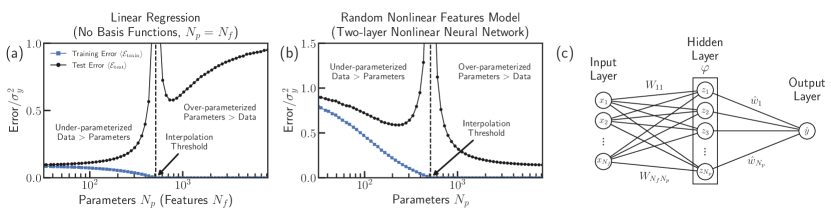
Figure 1: Double-descent phenomenon. (a)-(b) Examples of the average training error (blue squares) and test error (black circles) for two different models calculated via numerical simulations. In both models, the test error diverges when the training error reaches zero at the interpolation threshold, located where the number of parameters $N_{p}$ matches the number of points in the training data set $M$ (indicated by a black dashed vertical line). (a) In linear regression without basis functions, the number of features in the data $N_{f}$ matches the number of fit parameters $N_{p}$. (b) The random nonlinear features model (two-layer neural network where the parameters of the middle layer are random but fixed) decouples the number of features $N_{f}$ and the number of fit parameters $N_{p}$ by incorporating an additional “hidden layer” and transforms the data using a nonlinear activation function (e.g., ReLU), resulting in the canonical double-descent behavior. (c) Schematic of the model architecture for the random nonlinear features model. Numerical results are shown for a linear teacher model $y(\vec{\mathbf{x}})=\vec{\mathbf{x}}\cdot\vec{\boldsymbol{\beta}}+\varepsilon$, a signal-to-noise ratio of $\sigma_{\beta}^{2}\sigma_{X}^{2}/\sigma_{\varepsilon}^{2}=10$, and a small regularization parameter of $\lambda=10^{-6}$. The $y$-axes have been scaled by the variance of the training set labels $\sigma_{y}^{2}=\sigma_{\beta}^{2}\sigma_{X}^{2}+\sigma_{\varepsilon}^{2}$. Each point is averaged over at least $1000$ independent simulations trained on $M=512$ data points with small error bars indicating the error on the mean. In (b), there are less features than data points $N_{f}=M/4$. See Sec. II for precise definitions and Sec. S4 of Supplemental Material sup for additional simulation details.

Clearly, the classical picture provided by the bias-variance trade-off is incomplete. Classical statistics largely focuses on under-parameterized models which are simple enough that they have a nonzero training error. In contrast, Modern Deep Learning methods push model complexity past the interpolation threshold, the point at which the training error reaches zero Belkin et al. (2019); Geiger et al. (2019); Spigler et al. (2019); Mailman and Chakraborty (2011); Bahri et al. (2020). In the classical picture, approaching the interpolation threshold coincides with a large increase, or even divergence, in the test error via the variance. However, numerical experiments suggest that the predictive performance of over-parameterized models is better described by “double-descent” curves which extend the classic U-shape past the interpolation threshold to account for over-parameterized models with zero training error Belkin et al. (2019); Kobak [@hippopedoid] (2020); Loog et al. (2020). Surprisingly, if model complexity is increased past the interpolation threshold, the test error once again decreases, often resulting in over-parameterized models with even better out-of-sample performance than their under-parameterized counterparts [see Fig. 1(b)].

This double-descent behavior stands in stark contrast with the classical statistical intuition based on the bias-variance trade-off; both bias and variance appear to decrease past the interpolation threshold. Therefore, understanding this phenomenon requires generalizing the bias-variance decomposition to over-parameterized models. More broadly, explaining the unexpected success of over-parameterized models represents a fundamental problem in ML and modern statistics.

I.1 Relation to Previous Work

In recent years, many attempts have been made to understand the origins of this double-descent behavior via numerical and/or analytical approaches. While much of this work has relied on well constructed numerical experiments on complex Deep Learning models Zhang et al. (2017); Belkin et al. (2019); Spigler et al. (2019); Nakkiran et al. (2020), many theoretical studies have focused on a much simpler setting: the so-called “lazy training” regime. Previously, it was observed that in the limit of an infinitely wide network, the learning process appears to mimic that of an approximate kernel method in which the kernel used by the model to express the data – the Neural Tangent Kernel (NTK) – remains fixed Jacot et al. (2018); Lee et al. (2019). This stands in contrast to the so-called “feature training” regime in which the kernel evolves over time as the model learns the most informative way to express the relationships in the data Geiger et al. (2020).

Making use of the observation that the kernel remains approximately fixed in the lazy regime, many analytical studies have derived training and test errors for neural networks where the top layer is trained, but the middle layer(s) remained fixed, effectively reducing these models to linearized versions of regression or classificaiton with various types of nontrivial basis functions Adlam and Pennington (2020); Advani et al. (2020); Ba et al. (2020); Barbier et al. (2019); Bartlett et al. (2020); Belkin et al. (2020); Bibas et al. (2019); Deng et al. (2020); D’Ascoli et al. (2020a, b); Dereziński et al. (2020); Dhifallah and Lu (2020); Gerace et al. (2020); Hastie et al. (2019); Jacot et al. (2020); Kini and Thrampoulidis (2020); Lampinen and Ganguli (2019); Li et al. (2020); Liang and Rakhlin (2020); Liang et al. (2020); Liao et al. (2020); Lin and Dobriban (2021); Mitra (2019); Mei and Montanari (2021); Muthukumar et al. (2019); Nakkiran (2019); Xu and Hsu (2019); Yang et al. (2020). Furthermore, some of these studies have considered nonlinear data distributions Dhifallah and Lu (2020); Mei and Montanari (2021). Importantly, such studies have typically combined a fixed-kernel approach with specific choices of loss functions (e.g., mean-squared error) to guarantee convexity, while the loss landscapes of neural networks in practical settings are often highly non-convex Dauphin et al. (2014). Despite being limited to the lazy regime and convex loss landscapes, the closed-form solutions for the training and test error obtained for these models exhibit the double-descent phenomenon, demonstrating that many of the key features of more complex Deep Learning architectures can arise in much simpler settings.

A smaller subset of these studies have also attempted to extend these calculations to compute the bias-variance decomposition Adlam and Pennington (2020); Ba et al. (2020); D’Ascoli et al. (2020a, b); Dereziński et al. (2020); Hastie et al. (2019); Jacot et al. (2020); Li et al. (2020); Lin and Dobriban (2021); Mei and Montanari (2021); Nakkiran (2019); Yang et al. (2020). However, this literature is rife with qualitative and quantitative disagreements, and as a result, a consensus has not formed regarding many of the basic properties of bias and variance in over-parameterized models. Underlying these disagreements is the ubiquitous use of non-standard and varying definitions of bias and variance (see Sec. V.6 for an in-depth discussion).

For example, some studies consider a fixed design matrix for the training data set in the definitions of bias and variance, but not for the test set, resulting in an effective mismatch in their data distributions Adlam and Pennington (2020); Ba et al. (2020); Dereziński et al. (2020); Hastie et al. (2019); Jacot et al. (2020); Li et al. (2020); Mei and Montanari (2021). As a result, these studies do not even reproduce the classical bias-variance trade-off expected in the under-parameterized regime.

Meanwhile, other studies do not distinguish between sources of randomness stemming from the model architecture (e.g., due to initialization) and sampling of the training data set, inadvertently leading these analyses to derive the bias of ensemble models rather than the models actually under investigation Adlam and Pennington (2020); D’Ascoli et al. (2020a, b); Jacot et al. (2020); Lin and Dobriban (2021); Yang et al. (2020). Consequently, these studies have found that in the absence of regularization, the bias reaches a minimum at the interpolation threshold and then remains constant into the over-parameterized regime.

In fact, of these studies, closed-form expressions using the standard definitions of bias and variance have only been obtained for the simple case of linear regression without basis functions and a linear data distribution Nakkiran (2019). While this setting captures some qualitative aspects of the double-descent phenomenon [see Fig. 1(a)], it requires a one-to-one correspondence between features in the data and fit parameters and a perfect match between the data distribution and model architecture, making it difficult to understand, if and how these results generalize to more complicated statistical models.

In line with previous studies, in this work, we also focus on the lazy regime with a convex loss landscape, considering two different linear models that emulate many properties of more complicated neural network architectures (see next section). However, our approach differs in that we utilize the traditional definitions of bias and variance, allowing us to clear up much of the confusion surrounding the bias-variance decomposition in over-parameterized models. In this way, we connect Modern Deep Learning to the statistical literature of the last century and in doing so, gain proper intuition for the origins of the double-descent phenomenon.

I.2 Overview of Approach

In this work, we use methods from statistical physics to derive analytic results for bias and variance in the over-parameterized regime for two minimal model architectures. These models, whose behavior is depicted in Fig. 1, are linear regression (ridge regression without basis functions and in the limit where the regularization parameter goes to zero – often called “ridge-less regression” in the statistics and ML literature) and the random nonlinear features model (a two-layer neural network with an arbitrary nonlinear activation function where the top layer is trained and parameters for the intermediate layer are chosen to be random but fixed). We generate the data used to train both models using a non-linear “teacher model” where the labels are related to the features through a non-linear function (usually with additive noise). Using similar terminology, we often refer to the details of a model’s architecture as the “student model.” Crucially, the differences between the two models we consider allow us to disentangle the effects of model architecture on bias and variance versus effects arising from randomly sampling the underlying data distribution.

Linear regression is one of the simplest models in which the test error diverges at the interpolation threshold but then decreases in the over-parameterized regime [Fig. 1(a)]. Because this model uses the features in the data directly without modification (i.e., it lacks a hidden layer), it provides evidence that the process of randomly sampling the data itself plays an integral part in the double-descent phenomena. The random nonlinear features model [Figs. 1(b) and (c)] provides insight into the effects of filtering the features through an additional transformation, in effect, changing the way the model views the data. This disconnect between features and their representations in the model is crucial for understanding bias and variance in more complex over-parameterized models.

To treat these models analytically, we make use of the “zero-temperature cavity method” which has a long history in the physics of disordered systems and statistical learning theory Engel et al. (2001); Mézard and Parisi (2003); Ramezanali et al. (2015). In particular, our calculations follow the style of Ref. Mehta et al., 2019b and assume that the solutions can be described using a Replica-Symmetric Ansatz, which we confirm numerically. Our analytic results are exact in the thermodynamic limit where the number of data points $M$, the number of features in the data $N_{f}$, and the number of fit parameters (hidden features) $N_{p}$ all tend towards infinity. Crucially, when taking this limit, the ratios between these three quantities are assumed to be fixed and finite, allowing us to ask how varying these ratios and other model properties (such as linear versus nonlinear activation functions) affect generalization. We confirm that all our analytic expressions agree extremely well with numerical results, even for relatively small system sizes ($N_{f},N_{p},M\sim 10-1000$).

I.3 Summary of Major Results

Before proceeding further, we briefly summarize our major results:

• We derive analytic expressions for the test (generalization) error, training error, bias, and variance for both models using the zero-temperature cavity method.

• We show that both models exhibit a phase transition at an interpolation threshold to an interpolation regime where the training error is zero.

• In the under-parameterized regime, we find that the variance diverges as it approaches the interpolation threshold, leading to extremely large generalization error, while the bias either remains constant (linear regression) or decreases monotonically in a classical bias-variance trade-off (random nonlinear features model).

• In the over-parameterized regime, we find that the test error either decreases non-monotonically due to a decrease in variance and an increase in bias (linear regression) or decreases monotonically due to a monotonic decrease in both variance and bias, even in the absence of regularization (random nonlinear features model).

• We show that bias in over-parameterized models has two sources: error resulting from mismatches between the student and teacher models (i.e., the model is incapable of fully capturing the full data distribution) and incomplete sampling of the data’s feature space. We show that as a result of the latter case, one can have nonzero bias even if the student and teacher models are identical. We also show that bias decreases in the interpolation regime only if the number of features in the data remains fixed.

• We show that biased models can overfit even in the absence of noise. In other words, biased models can interpret signal as noise.

• We show that the zero-temperature susceptibilities that appear in our cavity calculations measure the sensitivity of a fitted model to small perturbations. We discuss how these susceptibilities can be used to identify phase transitions and are each related to different aspects of the double-descent phenomena.

• We combine these observations to provide a comprehensive intuitive explanation of the double-descent curves for test error observed in over-parameterized models, making connections to random matrix theory. In particular, we discuss how diverging test error stems from small eigenvalues in the Hessian, corresponding to poorly sampled directions in the space of input features for linear regression or the space of hidden features for the random nonlinear features model.

• We discuss why using the standard definitions of bias and variance are necessary to properly connect the double-descent phenomenon to the classical bias-variance trade-off.

I.4 Organization of Paper

In Sec. II, we start by providing the theoretical setup for both models and briefly summarize the methods we use to derive analytic expressions. In Sec. III, we provide precise definitions of bias and variance, taking great care to distinguish between different sources of randomness. In Sec. IV, we report our analytic results and compare them to numerical simulations. In Sec. V, we use these analytic expressions to understand how bias and variance generalize to over-parameterized models and also discuss the roles of the susceptibilities that arise as part of our cavity calculations. Finally, in Sec. VI, we conclude and discuss the implications of our results for modern ML methods.

II Theoretical Setup

II.1 Supervised Learning Task

In this work, we consider data points $(y,\vec{\mathbf{x}})$, each consisting of a continuous label $y$ paired with a set of $N_{f}$ continuous features $\vec{\mathbf{x}}$. To distinguish the features in the data from those in the model, we refer to $\vec{\mathbf{x}}$ as the “input features.” We frame the supervised learning task as follows: using the relationships learned from a training data set, construct a model to accurately predict the labels $y$ of new data points based on their input features $\vec{\mathbf{x}}$.

II.2 Data Distribution (Teacher Model)

We assume that the relationship between the input features and labels (the data distribution or teacher model) can be expressed as

$$y(\vec{\mathbf{x}}) =y^{*}(\vec{\mathbf{x}};\vec{\boldsymbol{\beta}})+\varepsilon$$ (1)

where $\varepsilon$ is the label noise and $y^{*}(\vec{\mathbf{x}};\vec{\boldsymbol{\beta}})$ is an unknown function representing the “true” labels. This function takes the features as arguments and combines them with a set of $N_{f}$ “ground truth” parameters $\vec{\boldsymbol{\beta}}$ which characterize the correlations between the features and labels.

We draw the input features for each data point independently and identically from a normal distribution with zero mean and variance $\sigma_{X}^{2}/N_{f}$. Normalizing the variance by $N_{f}$ ensures that the magnitude of each feature vector is independent of the number of features and that a proper thermodynamic limit exists. Note that in this work, we consider features that do not contain noise. We also choose each element of the ground truth parameters $\vec{\boldsymbol{\beta}}$ and the label noise $\varepsilon$ to be independent of the input features and mutually independent from one another, drawn from normal distributions with zero mean and variances $\sigma_{\beta}^{2}$ and $\sigma_{\varepsilon}^{2}$, respectively.

In this work, we restrict ourselves to a teacher model of the form

$$y^{*}(\vec{\mathbf{x}};\vec{\boldsymbol{\beta}})=\frac{\sigma_{\beta}\sigma_{X}}{\expectationvalue*{f^{\prime}}}f\quantity(\frac{\vec{\mathbf{x}}\cdot\vec{\boldsymbol{\beta}}}{\sigma_{X}\sigma_{\beta}})$$ (2)

where the function $f$ is an arbitrary nonlinear function and ${\expectationvalue*{f^{\prime}}=\frac{1}{\sqrt{2\pi}}\int_{-\infty}^{\infty}\differential he^{-\frac{h^{2}}{2}}f^{\prime}(h)}$ is a normalization constant chosen for convenience with prime notation used to indicate a derivative (see Sec. S1D of Supplemental Information sup ). We place a factor of $1/(\sigma_{X}\sigma_{\beta})$ inside the function $f$ so that its argument has unit variance, while the pre-factor $\sigma_{\beta}\sigma_{X}$ ensures that $y^{*}$ reduces to a linear teacher model ${y^{*}(\vec{\mathbf{x}})=\vec{\mathbf{x}}\cdot\vec{\boldsymbol{\beta}}}$ when $f(h)=h$. Furthermore, we assume both the labels and input features are centered so that $f$ has zero mean with respect to its argument. While the results we report hold for a general $f$ of this form, all figures show numerical simulations for a linear teacher model unless otherwise specified.

II.3 Model Architectures (Student Models)

We consider two different student models that we discuss in detail below: linear regression and the random nonlinear features model. A schematic of the network architecture for the latter model is depicted in Fig. 1(c). Both student models take the general form

$$\hat{y}(\vec{\mathbf{x}}) =\vec{\mathbf{z}}(\vec{\mathbf{x}})\cdot\hat{\mathbf{w}}.$$ (3)

where $\hat{\mathbf{w}}$ is a vector of fit parameters and $\vec{\mathbf{z}}(\vec{\mathbf{x}})$ is a vector of “hidden” features which each may depend on a combination of the input features $\vec{\mathbf{x}}$. The hidden features $\vec{\mathbf{z}}$ are effectively the representations of the data points from the perspective of the model.

Since we only fit the top layer of the network in both models, the number of fit parameters $N_{p}$ equals the number of hidden features, and Eq. (3) is equivalent to a linear model with basis functions. Despite its simplicity, we will show that this model reproduces much of the interesting behaviors observed in more complicated neural networks.

II.3.1 Linear Regression

For linear regression without basis functions [Fig. 1(a)], the representations of the features from the perspective of the model are simply the input features themselves so that $\vec{\mathbf{z}}(\vec{\mathbf{x}})=\vec{\mathbf{x}}$. In other words, the hidden and input features are identical, leading to exactly one fit parameter for each feature, $N_{p}=N_{f}$.

II.3.2 Random Nonlinear Features Model

In the random nonlinear features model [Fig. 1(b) and (c)], the hidden features for each data point are related to the input features via a random matrix $W$ of size $N_{f}\times N_{p}$ and a nonlinear activation function $\varphi$,

$$\vec{\mathbf{z}}(\vec{\mathbf{x}}) =\frac{1}{\expectationvalue*{\varphi^{\prime}}}\frac{\sigma_{W}\sigma_{X}}{\sqrt{N_{p}}}\varphi\quantity(\frac{\sqrt{N_{p}}}{\sigma_{W}\sigma_{X}}W^{T}\vec{\mathbf{x}}),$$ (4)

where $\varphi$ acts separately on each element of its input and ${\expectationvalue*{\varphi^{\prime}}=\frac{1}{\sqrt{2\pi}}\int_{-\infty}^{\infty}\differential he^{-\frac{h^{2}}{2}}\varphi^{\prime}(h)}$ is a normalization constant chosen for convenience (see Sec. S1D of Supplemental Information sup ). We take each element of $W$ to be independent and identically distributed, drawn from a normal distribution with zero mean and variance $\sigma_{W}^{2}/N_{p}$. The normalization by $N_{p}$ is chosen so that the magnitude of each hidden feature vector only depends on the ratio of the number of input features to parameters which we always take to be finite. We place a factor of $\sqrt{N_{p}}/(\sigma_{W}\sigma_{X})$ inside the activation function so that its argument has approximately unit variance, and a second pre-factor of $\sigma_{W}\sigma_{X}/\sqrt{N_{p}}$ in front of $\varphi$ to ensure that $\vec{\mathbf{z}}$ reduces to a linear model $\vec{\mathbf{z}}(\vec{\mathbf{x}})=W^{T}\vec{\mathbf{x}}$ when the activation function is linear [i.e., $\varphi(h)=h$]. We note that while this model is technically a linear model with a specific choice of basis functions, it is equivalent to a two-layer neural network where the weights of the middle layer are chosen to be random and only the top layer is trained. Although our analytic results hold for an arbitrary nonlinear activation function $\varphi$, all figures show results for ReLU activation where $\varphi(h)=\max(0,h)$.

II.4 Fitting Procedure

We train each model on a training data set consisting of $M$ data points, ${\mathcal{D}=\{(y_{a},\vec{\mathbf{x}}_{a})\}_{a=1}^{M}}$. For convenience, we organize the vectors of input features in the training set into an observation matrix $X$ of size $M\times N_{f}$ and define the length-$M$ vectors of training labels $\vec{\mathbf{y}}$, training label noise $\vec{\boldsymbol{\varepsilon}}$, and label predictions for the training set $\hat{\mathbf{y}}$. We also organize the vectors of hidden features evaluated on the input features of the training set, $\{\vec{\mathbf{z}}(\vec{\mathbf{x}}_{a})\}_{a=1}^{M}$, into the rows of a hidden feature matrix $Z$ of size $M\times N_{p}$.

Given a set of training data $\mathcal{D}$, we solve for the optimal values of the fit parameters $\hat{\mathbf{w}}$ by minimizing the standard loss function used for ridge regression,

$$L(\hat{\mathbf{w}};\mathcal{D}) =\frac{1}{2}\norm*{\Delta\vec{\mathbf{y}}}^{2}+\frac{\lambda}{2}\norm*{\hat{\mathbf{w}}}^{2},$$ (5)

where the notation $\norm*{\cdot}$ indicates an $L_{2}$ norm and ${\Delta\vec{\mathbf{y}}=\vec{\mathbf{y}}-\hat{\mathbf{y}}}$ is the vector of residual label errors for the training set. The first term is simply the mean squared error between the true labels and their predicted values, while the second term imposes standard $L_{2}$ regularization with regularization parameter $\lambda$. We will often work in the “ridge-less limit” where we take the limit $\lambda\rightarrow 0$.

II.5 Model Evaluation

To evaluate each model’s prediction accuracy, we measure the training and test (generalization) errors. We define the training error as the mean squared residual label error of the training data,

$$\mathcal{E}_{\mathrm{train}} =\frac{1}{M}\norm*{\Delta\vec{\mathbf{y}}}^{2}.$$ (6)

We define the interpolation threshold as the model complexity at which the training error becomes exactly zero (in the thermodynamic and ridge-less limits). Analogously, we define the test error as the mean squared error evaluated on a test data set, ${\mathcal{D}^{\prime}=\{(y_{a}^{\prime},\vec{\mathbf{x}}_{a}^{\prime})\}_{a=1}^{M^{\prime}}}$, composed of $M^{\prime}$ new data points drawn independently from the same data distribution as the training data,

$$\mathcal{E}_{\mathrm{test}} =\frac{1}{M^{\prime}}\norm*{\Delta\vec{\mathbf{y}}^{\prime}}^{2},$$ (7)

where $\Delta\vec{\mathbf{y}}^{\prime}=\vec{\mathbf{y}}^{\prime}-\hat{\mathbf{y}}^{\prime}$ is a length-$M^{\prime}$ vector of residual label errors between the vector of labels $\vec{\mathbf{y}}^{\prime}$ and their predicted values $\hat{\mathbf{y}}^{\prime}$ for the test set.

II.6 Exact Solutions

To solve for unique optimal solution, we set the gradient with respect to the fit parameters to zero, giving us a set of $N_{p}$ equations with $N_{p}$ unknowns,

$$0 =\partialderivative{L(\hat{\mathbf{w}})}{\hat{\mathbf{w}}}=-Z^{T}\Delta\vec{\mathbf{y}}+\lambda\hat{\mathbf{w}}.$$ (8)

Solving this set of equations results in a unique solution for the fit parameters,

$$\hat{\mathbf{w}} =\quantity[\lambda I_{N_{p}}+Z^{T}Z]^{-1}Z^{T}\vec{\mathbf{y}}.$$ (9)

For simplicity, we also take the ridge-less limit where $\lambda$ is infinitesimally small ($\lambda\rightarrow 0$). While our calculations do provide exact solutions for finite $\lambda$, the solutions in the limits of small $\lambda$ are much more insightful. In this limit, Eq. (9) and Eq. (3) approximate to

$$\hat{\mathbf{w}}\approx Z^{+}\vec{\mathbf{y}},\qquad\hat{y}(\vec{\mathbf{x}})\approx\vec{\mathbf{z}}(\vec{\mathbf{x}})\cdot Z^{+}\vec{\mathbf{y}}$$ (10)

where ⁺ denotes a Moore-Penrose inverse, or pseudoinverse.

II.7 Hessian Matrix

We note that the solution for the fit parameters in Eq. (9) depends on the matrix $Z^{T}Z$, which we refer to in the ridge-less limit as the Hessian matrix. The matrix $Z^{T}Z/M$ can be interpreted as an empirical covariance matrix of the hidden features sampled by the training set when the hidden features are centered. The authors of Ref. Advani et al. (2018) showed that for ridge regression, the divergence of the test error at the interpolation threshold can be naturally understood in terms of the spectrum of the Hessian. Inspired by this observation, we also explore the relationship between the eigenvalues of the Hessian and the double-descent phenomenon in our more general setting.

To do so, we reproduce the known eigenvalue distribution for the Hessian for both models. We note that in linear regression (no basis functions), the Hessian is simply a Wishart matrix whose eigenvalues follow the Marchenko-Pastur distribution Marčenko and Pastur (1967). The eigenvalue spectrum for the Hessian for the random nonlinear features model was explored in Ref. Pennington and Worah, 2019. For both models, we provide an alternative derivation of these spectra using the zero-temperature cavity method, allowing us to directly relate the eigenvalues of the Hessian matrix to the double-descent phenomenon.

II.8 Derivation of Closed-Form Solutions

While the expressions in the previous section are quite general, they hide much of the complexity of the problem and are difficult to analyze carefully. For this reason, we make use of the zero-temperature cavity method to find closed-form solutions for all quantities of interest. The zero-temperature cavity method has a long history in the physics of disordered systems and statistical learning theory and has been used to analyze the Hopfield model Mézard (2017) and more recently, compressed sensing Ramezanali et al. (2019); Barbier et al. (2019). The cavity method is an alternative to the more commonly used Replica Method or analyses based on Random Matrix Theory.

Like the Replica Method, finding closed-form solutions requires some additional assumptions. In particular, we assume that the solutions satisfy a Replica-Symmetric Ansatz (an assumption we confirm numerically by showing remarkable agreement between our analytic results and simulations). Furthermore, we work in the thermodynamic limit, where $N_{f},M,N_{p}\rightarrow\infty$ and keep terms to leading order in these quantities. Our results are exact under these assumptions.

To apply the zero-temperature cavity method, we start by defining the ratio of the number of input features to training data points $\alpha_{f}=N_{f}/M$ and the ratio of fit parameters to training data points $\alpha_{p}=N_{p}/M$. Next, we take the thermodynamic limit $N_{f},M,N_{p}\rightarrow\infty$, while keeping the ratios $\alpha_{f}$ and $\alpha_{p}$ finite. The essence of the cavity method is to expand the solutions of Eq. (8) with $M+1$ data points, $N_{f}+1$ features and $N_{p}+1$ parameters about the solutions where one quantity of each type has been removed: ${(M+1,N_{f}+1,N_{p}+1)\rightarrow(M,N_{f},N_{p})}$. These two solutions are then related using generalized susceptibilities. The result is a set of algebraic self-consistency equations that can be solved for the distributions of the removed quantities. The central limit theorem then allows us to approximate any quantity defined as a sum over a large number of random variables (e.g., the training and test errors) using just distributions for the removed quantities. Furthermore, using the procedure described in Ref. Cui et al. (2020), we use the susceptibilities resulting from the cavity method to reproduce the known closed-form solutions for the eigenvalues spectra of the Hessian matrices for both models. We refer the reader to the Supplemental Material sup for further details on these calculations.

III Bias-Variance Decomposition

The bias-variance decomposition separates test error into components stemming from three distinct sources: bias, variance, and noise. Informally, bias captures a model’s tendency to underfit, reflecting the erroneous assumptions made by a model that limit its ability to fully express the relationships underlying the data. On the other hand, variance captures a model’s tendency to overfit, capturing characteristics of the training set that are not a reflection of the data’s true relationships, but rather a by-product of random sampling (e.g., noise). As a result, a model with high variance may not generalize well to other data sets drawn from the same data distribution. Noise simply refers to an irreducible error inherent in generating a set of test data (i.e., the label noise in the test set).

Formally, bias represents the extent to which the label predictions $\hat{y}(\vec{\mathbf{x}})$ differs from the true function underlying the data distribution $y^{*}(\vec{\mathbf{x}})$ when evaluated on an arbitrary test data point $\vec{\mathbf{x}}$ and averaged over all possible training sets $\mathcal{D}$ Bishop (2006),

$$\mathrm{Bias}\quantity[\hat{y}(\vec{\mathbf{x}})] =\mathrm{E}_{\mathcal{D}}\quantity[\hat{y}(\vec{\mathbf{x}})]-y^{*}(\vec{\mathbf{x}}).$$ (11)

Likewise, variance formally measures the extent to which solutions of $\hat{y}(\vec{\mathbf{x}})$ for individual training sets $\mathcal{D}$ vary around the average Bishop (2006),

$$\mathrm{Var}\quantity[\hat{y}(\vec{\mathbf{x}})] =\mathrm{E}_{\mathcal{D}}\quantity[\hat{y}^{2}(\vec{\mathbf{x}})]-\mathrm{E}_{\mathcal{D}}\quantity[\hat{y}(\vec{\mathbf{x}})]^{2}.$$ (12)

Finally, the noise is simply the mean squared label noise associated with an arbitrary test data point $\vec{\mathbf{x}}$,

$$\mathrm{Noise} =\mathrm{E}\quantity[\varepsilon^{2}]=\sigma_{\varepsilon}^{2}.$$ (13)

The standard bias-variance decomposition relates these three quantities to the test error (averaged over all possible training sets $\mathcal{D}$). In addition, we must take into account the fact that the test error is evaluated on $M^{\prime}$ test data points, while the bias and variance only consider a single test point. Since each test point is drawn from the same distribution, averaging the test error over all possible test sets $\mathcal{D}^{\prime}$ is equivalent to averaging the bias and variance over the point $\vec{\mathbf{x}}$. This gives us the canonical bias-variance decomposition Bishop (2006),

$$\mathrm{E}_{\mathcal{D}^{\prime},\mathcal{D}}\quantity[\mathcal{E}_{\mathrm{test}}] =\mathrm{E}_{\vec{\mathbf{x}}}\quantity[\mathrm{Bias}^{2}[\hat{y}(\vec{\mathbf{x}})]]+\mathrm{E}_{\vec{\mathbf{x}}}\quantity[\mathrm{Var}[\hat{y}(\vec{\mathbf{x}})]]+\sigma_{\varepsilon}^{2}.$$ (14)

In this work, we also consider other sources of randomness (e.g., $\vec{\boldsymbol{\beta}}$ and $W$). To incorporate these random variables, we define the more general ensemble-averaged squared bias and variance, respectively, as

$$\begin{split}\expectationvalue*{\mathrm{Bias}^{2}[\hat{y}]}&=\mathrm{E}_{\vec{\boldsymbol{\beta}},W,\vec{\mathbf{x}}}\quantity[\mathrm{Bias}[\hat{y}(\vec{\mathbf{x}})]^{2}]\\ &=\mathrm{E}_{\vec{\boldsymbol{\beta}},W,\vec{\mathbf{x}}}\quantity[\quantity(\mathrm{E}_{X,\vec{\boldsymbol{\varepsilon}}}[\hat{y}(\vec{\mathbf{x}})]-y^{*}(\vec{\mathbf{x}}))^{2}]\end{split}$$ (15)

$$\begin{split}\expectationvalue*{\mathrm{Var}[\hat{y}]}&=\mathrm{E}_{\vec{\boldsymbol{\beta}},W,\vec{\mathbf{x}}}\quantity[\mathrm{Var}[\hat{y}(\vec{\mathbf{x}})]]\\ &=\mathrm{E}_{\vec{\boldsymbol{\beta}},W,\vec{\mathbf{x}}}\quantity[\mathrm{E}_{X,\vec{\boldsymbol{\varepsilon}}}[\hat{y}^{2}(\vec{\mathbf{x}})]-\mathrm{E}_{X,\vec{\boldsymbol{\varepsilon}}}[\hat{y}(\vec{\mathbf{x}})]^{2}]\end{split}$$ (16)

where we have explicitly included all random variables considered in this work. All analytic expressions we report are ensemble-averaged (denoted by angle brackets $\langle\cdot\rangle$) and utilize the ensemble-averaged bias-variance decomposition of the test error,

$$\expectationvalue{\mathcal{E}_{\mathrm{test}}} =\expectationvalue*{\mathrm{Bias}^{2}[\hat{y}]}+\expectationvalue*{\mathrm{Var}[\hat{y}]}+\sigma_{\varepsilon}^{2}.$$ (17)

By fixing any parameters that do not pertain to the random sampling process of the test or training data (in this case, $\vec{\boldsymbol{\beta}}$ and $W$), this formula properly reduces to the canonical bias-variance decomposition in Eq. (14).

IV Results

In this section, we provide analytic results for the training error, test error, bias, and variance, along with partial comparisons to numerical results. We limit ourselves to simply discussing major features of our closed-form solutions, deferring a discussion of the implications of these results to the next section. Analytic derivations and complete comparisons to numerical results are left to the Supplemental Material sup .

IV.1 General Solutions

We first report the forms of the solutions for arbitrary student and teacher models. We find that the training error, test error, bias, and variance take the general forms

$$\expectationvalue{\mathcal{E}_{\mathrm{train}}} =\expectationvalue*{\Delta y^{2}}$$ (18)

$$\expectationvalue{\mathcal{E}_{\mathrm{test}}} =\sigma_{X}^{2}\expectationvalue*{\Delta\beta^{2}}+\sigma_{\delta z}^{2}\expectationvalue*{\hat{w}}^{2}+\sigma_{\delta y^{*}}^{2}+\sigma_{\varepsilon}^{2}$$ (19)

$$\expectationvalue*{\mathrm{Bias}^{2}[\hat{y}]} =\sigma_{X}^{2}\expectationvalue*{\Delta\beta_{1}\Delta\beta_{2}}+\sigma_{\delta z}^{2}\expectationvalue*{\hat{w}_{1}\hat{w}_{2}}+\sigma_{\delta y^{*}}^{2}$$ (20)

$$\begin{split}\expectationvalue*{\mathrm{Var}[\hat{y}]}&=\sigma_{X}^{2}\quantity\big[\expectationvalue*{\Delta\beta^{2}}-\expectationvalue*{\Delta\beta_{1}\Delta\beta_{2}}]\\ &\qquad+\sigma_{\delta z}^{2}\quantity\big[\expectationvalue*{\hat{w}^{2}}-\expectationvalue*{\hat{w}_{1}\hat{w}_{2}}],\end{split}$$ (21)

which depend on five key ensemble-averaged quantities: $\expectationvalue*{\Delta y^{2}}$, $\expectationvalue*{\hat{w}^{2}}$, $\expectationvalue*{\Delta\beta^{2}}$, $\expectationvalue*{\hat{w}_{1}\hat{w}_{2}}$, and $\expectationvalue*{\Delta\beta_{1}\Delta\beta_{2}}$ (see Sec. S1E of Supplemental Material sup for detailed derivation). The first two quantities are the average of the squared training label errors $\expectationvalue*{\Delta y^{2}}$ and the average of the squared fit parameters $\expectationvalue*{\hat{w}^{2}}$. The third quantity $\expectationvalue*{\Delta\beta^{2}}$ measures a model’s accuracy in identifying the ground truth parameters $\vec{\boldsymbol{\beta}}$. To see this, we note that an estimate of the ground truth parameters for each model can be constructed from the fit parameters via the expression $\hat{\boldsymbol{\beta}}\equiv W\hat{\mathbf{w}}$, with residual parameter errors $\Delta\vec{\boldsymbol{\beta}}\equiv\vec{\boldsymbol{\beta}}-\hat{\boldsymbol{\beta}}$. Given these definitions, $\expectationvalue*{\Delta\beta^{2}}$ is then the average of the squared residual parameter errors. Finally, the quantities $\expectationvalue*{\hat{w}_{1}\hat{w}_{2}}$ and $\expectationvalue*{\Delta\beta_{1}\Delta\beta_{2}}$ measure the average covariances of a pair fit parameters or residual parameter errors, respectively, that have the same index but derive from models trained on different training sets drawn independently from the same data distribution.

In addition to these five ensemble averages, the above expressions also depend on the quantities $\sigma_{\delta y^{*}}^{2}$ and $\sigma_{\delta z}^{2}$ which characterize the degree of nonlinearity of the labels and hidden features, respectively. To define these quantities, we note that the nonlinear labels and hidden features considered in this work can each be decomposed into linear and nonlinear parts.

First, we decompose the true labels in Eq. (2) into two components that are statistically independent with respect to the distribution of input features, allowing us to express the teacher model as

$$y(\vec{\mathbf{x}})=\vec{\mathbf{x}}\cdot\vec{\boldsymbol{\beta}}+\delta y_{\mathrm{NL}}(\vec{\mathbf{x}})+\varepsilon.$$ (22)

The first term $\vec{\mathbf{x}}\cdot\vec{\boldsymbol{\beta}}$ captures the linear correlations between the input features $\vec{\mathbf{x}}$ and the true labels $y^{*}$ via the ground truth parameter $\vec{\boldsymbol{\beta}}$, while the second term $\delta y^{*}_{\mathrm{NL}}(\vec{\mathbf{x}})$ captures the nonlinear behavior of $y^{*}$ [defined as ${\delta y^{*}_{\mathrm{NL}}(\vec{\mathbf{x}})\equiv y^{*}(\vec{\mathbf{x}})-\vec{\mathbf{x}}\cdot\vec{\boldsymbol{\beta}}}$]. The nonlinear component has zero mean (since the labels are centered with zero mean) and we define its variance as $\sigma_{\delta y^{*}}^{2}$. Previously, this decomposition was implemented by noting that $\delta y^{*}_{\mathrm{NL}}(\vec{\mathbf{x}})$ behaves like an independent Gaussian process Dhifallah and Lu (2020); Mei and Montanari (2021). Here, we note that this approximation follows naturally in the thermodynamic limit from the relationship $\vec{\boldsymbol{\beta}}=\Sigma_{\vec{\mathbf{x}}}^{-1}\mathrm{Cov}_{\vec{\mathbf{x}}}[\vec{\mathbf{x}},y^{*}(\vec{\mathbf{x}})]$ where ${\Sigma_{\vec{\mathbf{x}}}\equiv\mathrm{Cov}_{\vec{\mathbf{x}}}[\vec{\mathbf{x}},\vec{\mathbf{x}}^{T}]}$ is the covariance matrix of the input features (see Sec. S1D of Supplemental Material sup ).

We also decompose the hidden features in Eq. (4) into three statistically independent components with respect to the distribution of input features,

$$\vec{\mathbf{z}}(\vec{\mathbf{x}})=\frac{\mu_{z}}{\sqrt{N_{p}}}\vec{\mathbf{1}}+W^{T}\vec{\mathbf{x}}+\delta\vec{\mathbf{z}}_{\mathrm{NL}}(\vec{\mathbf{x}}).$$ (23)

The first term $\mu_{Z}/\sqrt{N_{p}}\vec{\mathbf{1}}$ is the mean of each hidden feature where $\vec{\mathbf{1}}$ is a length-$N_{p}$ vector of ones. Analogously to the label decomposition, the second term $W^{T}\vec{\mathbf{x}}$ captures the linear correlations between the input features $\vec{\mathbf{x}}$ and the hidden features $\vec{\mathbf{z}}(\vec{\mathbf{x}})$ via the matrix of parameters $W$, while the third term $\delta\vec{\mathbf{z}}_{\mathrm{NL}}(\vec{\mathbf{x}})$ captures the remaining nonlinear behavior of $\vec{\mathbf{z}}(\vec{\mathbf{x}})$ [defined as ${\delta\vec{\mathbf{z}}_{\mathrm{NL}}(\vec{\mathbf{x}})\equiv\vec{\mathbf{z}}(\vec{\mathbf{x}})-\mu_{z}\vec{\mathbf{1}}/\sqrt{N_{p}}-W^{T}\vec{\mathbf{x}}}$]. The nonlinear component has zero mean and we define its total variance as $\sigma_{\delta z}^{2}$. Like the nonlinear teacher model, it was previously observed that the nonlinear component of the hidden features behaves like an independent Gaussian process Goldt et al. (2020), and this decomposition has since been used as a common trick to obtain closed-form solutions for nonlinear models. Here, we again note that this approximation follows naturally in the thermodynamic limit from the relationship $W=\Sigma_{\vec{\mathbf{x}}}^{-1}\mathrm{Cov}_{\vec{\mathbf{x}}}[\vec{\mathbf{x}},\vec{\mathbf{z}}(\vec{\mathbf{x}})^{T}]$ (see Sec. S1D of Supplemental Material sup ).

We find the variance of the nonlinear components of the labels and hidden features, respectively, to be

$$\sigma_{\delta y^{*}}^{2} =\sigma_{\beta}^{2}\sigma_{X}^{2}\Delta f, \Delta f =\frac{\expectationvalue*{f^{2}}-\expectationvalue*{f^{\prime}}^{2}}{\expectationvalue*{f^{\prime}}^{2}}$$ (24)

$$\sigma_{\delta z}^{2} =\sigma_{W}^{2}\sigma_{X}^{2}\Delta\varphi, \Delta\varphi =\frac{\expectationvalue*{\varphi^{2}}-\expectationvalue*{\varphi}^{2}-\expectationvalue*{\varphi^{\prime}}^{2}}{\expectationvalue*{\varphi^{\prime}}^{2}},$$ (25)

where the quantities $\expectationvalue*{f^{2}}$, $\expectationvalue*{f^{\prime}}$, $\expectationvalue*{\varphi^{2}}$, $\expectationvalue*{\varphi}$, $\expectationvalue*{\varphi^{\prime}}$ are integrals of the form

$$\expectationvalue*{g} =\frac{1}{\sqrt{2\pi}}\int\limits_{-\infty}^{\infty}\differential he^{-\frac{1}{2}h^{2}}g(h)$$ (26)

with derivatives indicated via prime notation [e.g., ${f^{\prime}=df(h)/dh}$]. The differences $\Delta f$ and $\Delta\varphi$ measure the ratio of the variances of each nonlinear component to its linear counterparts and go to zero in the linear limit. For ReLU activation, $\varphi(h)=\max(h,0)$, we find $\expectationvalue*{\varphi^{2}}=1/2$, $\expectationvalue*{\varphi}=1/\sqrt{2\pi}$, and $\expectationvalue*{\varphi^{\prime}}=1/2$, resulting in $\Delta\varphi=1-2/\pi$.

We derive Eqs. (19)-(21) by decomposing the labels and hidden features of the test data (see Sec. S1E in Supplemental Information sup ). As a result, we can identify what elements of the test data lead to each term in these expressions. We observe that terms proportional to $\sigma_{X}^{2}$ capture error arising from the linear components of the test data’s labels and hidden features. More precisely, these terms measure error due to the mismatch between the linear components of the test labels and a model’s predictions based solely on the linear components of the test data’s hidden features ${\vec{\mathbf{x}}\cdot\Delta\beta=\vec{\mathbf{x}}\cdot\vec{\boldsymbol{\beta}}-\vec{\mathbf{x}}\cdot W\hat{\mathbf{w}}}$. In contrast, terms proportional to $\sigma_{\delta y^{*}}^{2}$ and $\sigma_{\delta z}^{2}$ represent errors due to the nonlinear components of the test data’s labels and hidden features, respectively. Since the model is linear in the fit parameters, it cannot fully capture nonlinear relationships in the test data that deviate from those observed in the training set.

Finally, we note that the decomposition of the labels in Eq. (22) suggests that each key quantity, along with total train error, test error, bias, and variance, decompose into contributions from the different parts of the training labels. Since each term is statistically independent, the contribution of each is proportional to its respective variance, allowing us to simply read off the sources of each type of error from our analytic results. In particular, the linear and nonlinear components of the labels give rise to terms proportional to $\sigma_{\beta}^{2}\sigma_{X}^{2}$ and $\sigma_{\delta y^{*}}^{2}$, respectively, while the label noise gives rise to terms proportional to $\sigma_{\varepsilon}^{2}$.

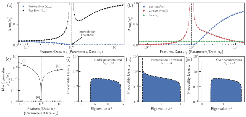
Figure 2: Linear Regression (No Basis Functions). Analytic solutions for the ensemble-averaged (a) training error (blue squares) and test error (black circles), and (b) bias-variance decomposition of test error with contributions from the squared bias (blue squares), variance (red squares), and test set label noise (green triangles), plotted as a function of $\alpha_{f}=N_{f}/M$ (or equivalently, $\alpha_{p}=N_{p}/M$). Analytic solutions are indicated as dashed lines with numerical results shown as points with small error bars indicating the error on the mean. In each panel, a black dashed vertical line marks the interpolation threshold $\alpha_{f}=1$. (c) Analytic solution for the minimum eigenvalue $\sigma_{\min}^{2}$ of the Hessian matrix $Z^{T}Z$. Examples of the eigenvalue distributions are shown (i) in the under-parameterized regime with $\alpha_{f}=1/8$, (ii) at the interpolation threshold, $\alpha_{f}=1$, and (iii) in the over-parameterized regime with $\alpha_{f}=8$. Analytic solutions for the distributions are depicted as black dashed curves with numerical results shown as blue histograms. See Sec. S4 of Supplemental Material sup for additional simulation details.

IV.2 Linear Regression

Here, we present results for linear regression (no basis functions). Generally, our solutions are most naturally expressed in terms of ${\alpha_{f}=N_{f}/M}$, the ratio of input features to training data points, and $\alpha_{p}=N_{p}/M$, the ratio of fit parameters to training data points. However, in this case, the input and hidden features coincide ($N_{f}=N_{p}$), so all expressions depend only on $\alpha_{f}$. The ensemble-averaged training error, test error, bias, and variance for linear regression are:

$$\expectationvalue{\mathcal{E}_{\mathrm{train}}} =\left\{\begin{array}[]{c}(\sigma_{\varepsilon}^{2}+\sigma_{\delta y^{*}}^{2})(1-\alpha_{f})\\ 0\end{array}\right. \begin{array}[]{l}\mbox{\quad if\quad}N_{f}<M\\ \mbox{\quad if\quad}N_{f}>M\end{array}$$ (31)

$$\expectationvalue{\mathcal{E}_{\mathrm{test}}} =\left\{\begin{array}[]{c}(\sigma_{\varepsilon}^{2}+\sigma_{\delta y^{*}}^{2})\frac{1}{(1-\alpha_{f})}\\ \sigma_{\beta}^{2}\sigma_{X}^{2}\frac{(\alpha_{f}-1)}{\alpha_{f}}+(\sigma_{\varepsilon}^{2}+\sigma_{\delta y^{*}}^{2})\frac{\alpha_{f}}{(\alpha_{f}-1)}\end{array}\right. \begin{array}[]{l}\mbox{\quad if\quad}N_{f}<M\\ \mbox{\quad if\quad}N_{f}>M\end{array}$$ (36)

$$\expectationvalue*{\mathrm{Bias}^{2}[\hat{y}]} =\left\{\begin{array}[]{c}\sigma_{\delta y^{*}}^{2}\\ \sigma_{\beta}^{2}\sigma_{X}^{2}\frac{(\alpha_{f}-1)^{2}}{\alpha_{f}^{2}}+\sigma_{\delta y^{*}}^{2}\end{array}\right. \begin{array}[]{l}\mbox{\quad if\quad}N_{f}<M\\ \mbox{\quad if\quad}N_{f}>M\end{array}$$ (41)

$$\expectationvalue*{\mathrm{Var}[\hat{y}]} =\left\{\begin{array}[]{c}(\sigma_{\varepsilon}^{2}+\sigma_{\delta y^{*}}^{2})\frac{\alpha_{f}}{(1-\alpha_{f})}\\ \sigma_{\beta}^{2}\sigma_{X}^{2}\frac{(\alpha_{f}-1)}{\alpha_{f}^{2}}+(\sigma_{\varepsilon}^{2}+\sigma_{\delta y^{*}}^{2})\frac{1}{(\alpha_{f}-1)}\end{array}\right. \begin{array}[]{l}\mbox{\quad if\quad}N_{f}<M\\ \mbox{\quad if\quad}N_{f}>M.\end{array}$$ (46)

In writing these expressions, we have taken the ridge-less limit, $\lambda\rightarrow 0$ (when a quantity is reported as zero, leading terms of order $\lambda^{2}$ are reported in Sec. S1F of the Supplemental Material sup ).

In Fig. 2(a), we plot the expressions for the training and test error in Eqs. (31) and (36) with comparisons to numerical results for a linear teacher model $\sigma_{\delta y^{*}}^{2}=0$. We find that the model’s behavior falls into two broad regimes, depending on whether $\alpha_{f}>1$ or $\alpha_{f}<1$ (or equivalently, $\alpha_{p}>1$ or $\alpha_{p}<1$). In Fig. 2(a), we observe that below $\alpha_{f}=1$, the training error is finite, decreasing monotonically as $\alpha_{f}$ increases until reaching zero at $\alpha_{f}=1$. Beyond this threshold, the addition of extra features/parameters has no effect and the training error remains pinned at zero. Thus, $\alpha_{f}=1$ corresponds to the interpolation threshold, separating the regions where the model has zero and nonzero training error, i.e., the under- and over-parameterized regimes. At the interpolation threshold, the test error diverges [Fig. 2(a)], indicative of a phase transition based on the divergence of the corresponding susceptibilities in the cavity equations (see Sec. V.5 and Sec. S1F of Supplemental Material sup ).

The bias and variance, reported in Eqs. (41) and (46), are plotted in Fig. 2(b). When $\alpha_{f}\leq 1$, the bias is zero for a linear teacher model. This can be understood by noting that the teacher and student models match in this case and there are more data points than parameters (i.e., we are working in a regime where intuitions for classical statistics apply). In this regime, the variance increases monotonically as $\alpha_{f}$ is increased, diverging at the interpolation threshold as the model succumbs to overfitting. However, when $\alpha_{f}>1$, the variance exhibits the opposite behavior, decreasing monotonically as $\alpha_{f}$ is increased. The bias, on the other hand, increases monotonically towards the limit $\sigma_{\beta}^{2}\sigma_{X}^{2}+\sigma_{\delta y^{*}}^{2}$ as $\alpha_{f}$ goes to infinity. Consequently, the test error in the over-parameterized regime is characterized by a surprising “inverted bias-variance trade-off” where the bias increases with model complexity while the variance decreases.

In the solutions for the training error, test error, and variance, we observe that the error due to the nonlinear label components (proportional to $\sigma_{\delta y^{*}}^{2}$) always appears as an additive component to the errors stemming from the label noise (proportional to $\sigma_{\varepsilon}^{2}$). However, unlike the label noise, the nonlinear label variance $\sigma_{\delta y^{*}}^{2}$ also appears in the bias as an additional constant irreducible term that arises as a result of attempting to fit a nonlinear data distribution with a model that is linear in the fit parameters.

Finally, in Fig. 2(c), we report the minimum nonzero eigenvalue $\sigma_{\min}^{2}$ of the Hessian matrix $Z^{T}Z$, with examples of the full eigenvalue spectrum shown in Figs. 2(i)-(iii). Since $Z^{T}Z=X^{T}X$ for our model of linear regression, the eigenvalue spectrum is simply the Marchenko-Pastur distribution (see Sec. S2A of Supplemental Material for derivation). Importantly, we find the interpolation threshold $\alpha_{f}=1$ coincides with the point at which $\sigma_{\min}^{2}$ goes to zero. In the under-parameterized regime, there is a finite gap in the eigenvalue spectrum, with no small eigenvalues. In the over-parameterized, there is also a finite gap, but instead between the bulk of the spectrum and a buildup of eigenvalues at exactly zero. We discuss the implications of these findings later in Sec. V.2.

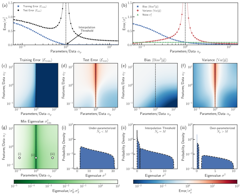
Figure 3: Random Nonlinear Features Model (Two-layer Neural Network). Analytic solutions for the ensemble-averaged (a) training error (blue squares) and test error (black circles), and (b) bias-variance decomposition of test error with contributions from the squared bias (blue squares), variance (red squares), and test set label noise (green triangles), plotted as a function of $\alpha_{p}=N_{p}/M$ for fixed $\alpha_{f}=N_{f}/M=1/4$. Analytic solutions are indicated as dashed lines with numerical results shown as points. Analytic solutions as a function of both $\alpha_{p}$ and $\alpha_{f}$ are also shown for the the ensemble-averaged (c) training error, (d) test error, (e) squared bias, and (f) variance. In all panels, a black dashed line marks the boundary between the under- and over-parameterized regimes at $\alpha_{p}=1$. (g) Analytic solution for the minimum eigenvalue $\sigma_{\min}^{2}$ of the Hessian matrix $Z^{T}Z$. Examples of the eigenvalue distributions are shown (i) in the under-parameterized regime with $\alpha_{p}=1/8$, (ii) at the interpolation threshold, $\alpha_{p}=1$, and (iii) in the over-parameterized regime with $\alpha_{p}=8$, all for $\alpha_{p}=1/4$. Analytic solutions for the distributions are shown as blacked dashed curves with numerical results shown as blue histograms. See Sec. S4 of Supplemental Material sup for additional simulation details.

IV.3 Random Nonlinear Features Model

Unlike the solutions for linear regression, the analytic expressions for the random nonlinear features model are not so simple, so we defer these expressions to the Appendix. In Fig. 3(a) and (b) we plot the training error, test error, bias, and variance as a function of $\alpha_{p}=N_{p}/M$ for fixed $\alpha_{f}<1$ (more data points $M$ than input features $N_{f}$), while in Figs. 3(c)-(f), we plot all quantities as a function of both $\alpha_{p}$ and $\alpha_{f}$. In all plots, we depict the special case of a linear teacher model $\sigma_{\delta y^{*}}^{2}=0$ and ReLU activation $\varphi(h)=\max(h,0)$. Analogously to linear regression, the nonlinear model has two distinct regimes separated by the line $\alpha_{p}=1$. In Fig. 3(c), we find that the training error is finite when $\alpha_{p}<1$ and goes to zero when $\alpha_{p}\geq 1$, marking the boundary $\alpha_{p}=1$ as the interpolation threshold. Fig. 3(d) shows that the test error diverges at each point along this boundary and no longer diverges when $\alpha_{f}=1$ as in the linear case [Fig. 2(a)]. However, we do still find that the divergence in the test error is associated with a phase transition indicated by diverging susceptibilities (see Sec. V.5 and Appendix).

In addition, the test error only displays a small qualitative difference between the regimes where $\alpha_{f}<1$ and $\alpha_{f}>1$. We find that the test error only shows a canonical double-descent behavior when $\alpha_{f}<1$ [Fig 3(d)]. As in linear regression, the variance [Fig. 3(f)], accounts for the divergence of the test error at the phase boundaries, while the bias [Fig. 3(e)] remains finite, decreasing monotonically for all $\alpha_{p}$. However, unlike linear regression, the bias of the nonlinear model never reaches zero, even for a linear teacher model. Furthermore, the closed-form solutions show that the nonlinear components of the labels $\sigma_{\delta y^{*}}^{2}$ contribute in the same way as in the two linear models, adding a small constant irreducible bias [Eq. (20)], along with an additive component to the label noise (see Appendix).

Finally, in Fig. 3(g), we report the minimum nonzero eigenvalue $\sigma_{\min}^{2}$ of the Hessian matrix $Z^{T}Z$ as a function of both $\alpha_{p}$ and $\alpha_{f}$ (see Sec. S2B of Supplemental Material for derivation of analytic results). We find that $\sigma_{\min}^{2}$ approaches zero along the entire interpolation boundary $\alpha_{p}=1$. In Figs. 3(i)-(iii), we show examples of the full eigenvalue spectrum for $\alpha_{f}<1$ for the under- and over-parameterized regimes, along with the interpolation threshold. We find that the spectrum in the under-parameterized regime displays a finite gap that goes to zero near the interpolation threshold. In the over-parameterized regime, we find that although the gap between the buildup of eigenvalues at zero and the nonzero eigenvalues is much smaller, it is still finite. Interestingly, we also find that additional gaps can appear in the eigenvalue distribution between sets of finite-valued eigenvalues, which likely reflects the fact that ReLU activation functions result in a large fraction of zero-valued entries in $Z$.

V Understanding bias and variance in over-parameterized models

Having presented our analytic results, we now discuss the implications of our calculations for understanding bias and variance in a more general setting. Our discussion emphasizes the qualitatively new phenomena that are present in over-parameterized models.

V.1 Two sources of bias: Imperfect models and incomplete exploration of features

Traditionally, bias is viewed as a symptom of a model making incorrect assumptions about the data distribution (a mismatch between the teacher and student models). However, our calculations show that this description of the origin of bias is incomplete. A striking feature of our results is that over-parameterized models can be biased even if our statistical models are expressive enough to fully capture all relationships underlying the data. In fact, linear regression shows us that one can have a nonzero bias even if the student and teacher models are identical [e.g., $f(h)=h$]. Even when the student and teacher model are the same, the bias is nonzero if there are more input features $N_{f}$ than data points $M$ [see $\alpha_{f}>1$ region of Fig. 2(b)].

To better understand this phenomenon, it is helpful to think of the input features as spanning an $N_{f}$-dimensional space. The training data can be embedded in this $N_{f}$-dimensional input feature space by considering the eigenvectors, or principal components, of the empirical covariance matrix of input features $X^{T}X/M$, with $X$ defined as the $M\times N_{f}$ design matrix whose rows correspond to training data points and columns to input features (see Sec. II). When there are more data points than input features ($M>N_{f}$), the training data will typically span the entire $N_{f}$-dimensional input feature space (i.e., the principal components of $X^{T}X$ generically span all of input feature space). In contrast, when there are fewer training data points than input features ($M<N_{f}$), the training data will typically span only a fraction of the entire input feature space (i.e., the principal components will span a subspace of the full $N_{f}$-dimensional input feature space). For this reason, when $M<N_{f}$ the model is “blind” to data that varies along these unsampled directions. Consequently, any predictions the model makes about these directions will reflect assumptions implicitly or explicitly built into the model rather than relationships learned from the training data set. This can result in a nonzero bias even when the teacher and student models are identical.

In the random nonlinear features model, the nonlinear activation function makes it impossible to perfectly represent the input features via the hidden features, even for a linear teacher model. While increasing the number of hidden features does reduce bias, the nonlinear model is never able to perfectly capture the linear nature of the data distribution and is always biased. Similarly, neither model is able to express the nonlinear components of the labels for a nonlinear teacher model, resulting in a constant, irreducible bias in both cases.

Finally, we wish to point out that, unlike some previous studies, we find that the bias never diverges Adlam and Pennington (2020); Ba et al. (2020); Mei and Montanari (2021), including at the interpolation transition, nor does it reach a minimum at the transition, remaining constant into the over-parameterized regime in the ridge-less limit Adlam and Pennington (2020); D’Ascoli et al. (2020a, b); Lin and Dobriban (2021). Instead, we find that the bias remains finite and decreases monotonically, even in the absence of regularization.

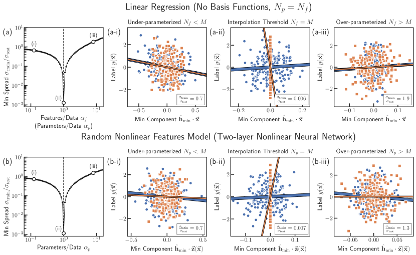
Figure 4: Poorly sampled directions in space of features lead to overfitting. Demonstrations of this phenomenon are shown for (a) linear regression and (b) the random nonlinear features model. Columns (i), (ii), and (iii) correspond to models which are under-parameterized, exactly at the interpolation threshold, or over-parameterized, respectively. In each example, the relationship between the labels and the projection of their associated input or hidden features onto the minimum principal component $\hat{\mathbf{h}}_{\min}$ of $Z^{T}Z$ is depicted for a set of training data (orange squares) and a test set (blue circles). Orange lines indicate the relationship learned by a model from the training set, while the expected relationship for an average test set is shown as a blue line. In the left-most column, the spread (standard deviation) of an average training set along the $x$-axis, $\sigma_{\mathrm{train}}^{2}=\sigma_{\min}^{2}/M$, is plotted relative to the spread that would be expected for an average test set, $\sigma_{\mathrm{test}}^{2}$, for simulated data as a function of $\alpha_{p}$. Smaller values are associated with lower prediction accuracy on out-of-sample data, coinciding with small eigenvalues in $Z^{T}Z$. All results are shown for a linear teacher model. See Supplemental Material sup for analytic derivations of learned and expected relationships and spreads along minimum principal components (Sec. S3), along with additional details of numerical simulations (Sec. S4).

V.2 Variance: Overfitting stems from poorly sampled direction in space of feature

Variance measures the tendency of a model to overfit, or attribute too much significance to, aspects of the training data that do not generalize to other data sets. Even when all data is drawn from the same distribution, the predictions of a trained model can vary depending on the details of each particular training set. More specifically, a model may exhibit high variance when a direction in feature space is present in the training data, but not sampled well enough to reflect its true nature in the underlying data distribution. When presented with new data that has a significant contribution along this under-sampled direction, the model is forced to extrapolate (often incorrectly) based on the little information it can glean from the training set.

In linear regression, the empirical variance along each principal direction is explicitly measured by its associated eigenvalue in the empirical covariance matrix $X^{T}X/M$. Generally, a model’s variance will be dominated by the most poorly sampled principal direction, or minimum component $\hat{\mathbf{h}}_{\min}$, corresponding to the smallest nonzero eigenvalue $\sigma_{\min}^{2}$ of $X^{T}X$. The projection of an arbitrary data point $\vec{\mathbf{x}}$ onto $\hat{\mathbf{h}}_{\min}$ can be found by taking a dot product, $\hat{\mathbf{h}}_{\min}\cdot\vec{\mathbf{x}}$. The observed variance of $\hat{\mathbf{h}}_{\min}\cdot\vec{\mathbf{x}}$ for a given training set is $\sigma^{2}_{\mathrm{train}}=\sigma_{\min}^{2}/M$. For comparison, we define the true, or expected, variance of $\hat{\mathbf{h}}_{\min}\cdot\vec{\mathbf{x}}$ for an average test set as $\sigma^{2}_{\mathrm{test}}$, representing data points drawn from the full data distribution (see Sec. S3 of Supplemental Material sup ).

The first row of Fig. 4 shows how observing a small variance along a particular direction sampled by the training data can lead to overfitting in linear regression. In Fig. 4(a), we plot the average ratio $\sigma_{\mathrm{train}}/\sigma_{\mathrm{test}}$ as a function of $\alpha_{f}$ for simulated data. In Figs. 4(a-i)-(a-iii), we then plot the labels $y$ versus $\hat{\mathbf{h}}_{\min}\cdot\vec{\mathbf{x}}$ for the training set (orange points) and an equally-sized test data set (blue points), representative of the full data distribution. In each panel, the relationship between the labels and $\hat{\mathbf{h}}_{\min}\cdot\vec{\mathbf{x}}$ as predicted by the model based on the training set is depicted as an orange line. For comparison, we also show the expected relationship for an average test set as a blue line, representing the true relationship underlying the data (see Sec. S3 of Supplemental Material sup for explicit formulas).

In Fig. 4(a-i), we see that when the model is under-parameterized ($N_{f}<M$), the spread of the training set along the minimum component is comparable to that of the test set ($\sigma_{\mathrm{train}}/\sigma_{\mathrm{test}}=0.7$). Because there are more data points than input features, many of the data points are likely to contain significant contributions from each direction, including the minimum component, corresponding to a finite gap in the corresponding eigenvalue distribution depicted in Fig. 2(c-i). As a result, the training set will provide the model with an accurate representation of the data distribution along this direction in feature space. In this case, we see that the model is able to closely approximate the true relationship in the data even in the presence of noise.

However, at the interpolation threshold when the number of input features equals the number of data points ($N_{f}=M$), Fig. 4(a-ii) shows that the spread of the training data points along the minimum component is very narrow compared to the test data ($\sigma_{\mathrm{train}}/\sigma_{\mathrm{test}}\approx 0.006$), while in Fig. 2(c-ii), we observe that the gap in the eigenvalue distribution disappears. In this case, the training set contains a very small, but insufficient, amount of information about the data distribution along this direction. This poor sampling causes the model to overfit the noise of the training set, resulting in a slope that is much larger than that of the true relationship. When presented with a new data point with a significant contribution along $\hat{\mathbf{h}}_{\min}$, the model will be forced to extrapolate beyond the narrow range of $\hat{\mathbf{h}}_{\min}\cdot\vec{\mathbf{x}}$ observed in the training set. This extrapolation will hamper the model’s ability to generalize, leading to inaccurate predictions that are highly dependent on the precise details of the noise sampled by the training set.

Surprisingly, we find in Fig. 4(a-iii) that further increasing the number of features so that the model becomes over-parameterized ($N_{f}>M$) actually increases the spread in the training data along the minimum component ($\sigma_{\mathrm{train}}/\sigma_{\mathrm{test}}\approx 1.9$), reducing the effects of overfitting. When there are more features than data points, each data point is likely to explore a never-before-seen combination of features. Naively, one would expect this to leave many of the directions poorly sampled. However, because the norm of each data point is approximately the same in the thermodynamic limit, the fact that each data point is different means that all are likely to make independent contributions of different sizes to the sampled directions, including $\hat{\mathbf{h}}_{\min}$. Even if this means only a single data point contributes to a particular component, this contribution must be of significant size for the data point to be independent of the rest. So while some directions are not represented in the training set at all, the ones that are present are typically well-represented by at least one – if not many – data points, providing a sufficient amount of signal (or spread) to reveal relationships in the underlying distribution. Consequently, the model is able to learn the true relationship between the labels and features, just as in the under-parameterized case. We observe this phenomenon directly in the eigenvalue distribution in Fig. 2(c-iii), with a buildup of eigenvalues at exactly zero corresponding to unsampled directions accompanied by a finite gap separating these eigenvalues from the rest of the distribution. This is the underlying reason that the variance decreases with model complexity beyond the interpolation threshold. A similar observation was made in Ref. Advani et al., 2020 in the context of ridge regression using methods from Random Matrix Theory.

In the second row of Fig. 4, we demonstrate that the same patterns also lead to overfitting in the random nonlinear features model, indicating that the intuition gained from linear regression translates directly to more complex settings. In this case, the model can be interpreted as indirectly sampling the data distribution via the empirical covariance matrix of hidden features $Z^{T}Z/M$. We calculate the minimum component $\hat{\mathbf{h}}_{\min}$ as the principal component of $Z^{T}Z$ with the smallest eigenvalue. In Figs. 4(b-i)-(b-iii), we plot the labels $y$ versus the projection of each data point’s hidden features $\vec{\mathbf{z}}$ onto this minimum component $\hat{\mathbf{h}}_{\min}\cdot\vec{\mathbf{z}}$, with the ratio $\sigma_{\mathrm{train}}/\sigma_{\mathrm{test}}$ shown in Fig. 4(b). In contrast to linear regression, we see that overfitting results from poorly sampling – or observing very limited spread along – a direction in the space of hidden features rather than input features. In the random nonlinear features model, overfitting is most pronounced when the number of hidden features matches the number of data points at the interpolation threshold ($N_{p}=M$), where the gap in the eigenvalue distribution at zero disappears [Fig. 3(g-ii)].

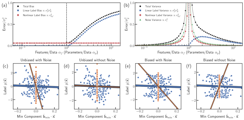
Figure 5: Biased models can interpret signal as noise. (a) The total bias (black circles) with contributions from the linear label components (blue squares) and nonlinear label components (red diamonds), and the (b) the total variance (black circles) with contributions from the linear label components (blue squares), nonlinear label components (red diamonds), and the label noise (green triangles) are shown for linear regression with a nonlinear teacher model $f(h)=\tanh(h)$ [see Eq. (2)]. Analytic solutions are indicated as dashed lines with numerical results shown as points. Contributions from the linear label components, nonlinear label components, and label noise are found by identifying terms in the analytic solutions proportional to $\sigma_{\beta}^{2}\sigma_{X}^{2}$, $\sigma_{\delta y^{*}}^{2}$, and $\sigma_{\varepsilon}^{2}$, respectively. Each source of bias acts as effective noise, giving rise to a corresponding source of variance. The effects of this phenomenon on the relationships learned by a linear regression model are depicted at the interpolation threshold for an unbiased model with linear data, $f(h)=h$, (c) with noise and (d) without noise, and for a biased model with nonlinear data, $f(h)=\tanh(h)$, (e) with noise and (f) without noise. In each example, the relationship between the labels and the projection of their associated input features onto the minimum principal component $\hat{\mathbf{h}}_{\min}$ of $X^{T}X$ is depicted for a set of training data (orange squares) and a test set (blue circles). Orange lines indicate the relationship learned by a model from the training set, while the expected relationship for an average test set is shown as a blue line. See Supplemental Material sup for analytic derivations of learned and expected relationships (Sec. S3), along with additional details of numerical simulations (Sec. S4).

V.3 Biased models can interpret signal as noise

Typically, variance is attributed to overfitting inconsistencies in the labels due to noise in the training set. Indeed, we observe that the contribution to the variance due to noise is nonzero in each model. Surprisingly, we also find that overfitting can occur in the absence of noise when a model is biased. In each model, we observe a direct correspondence between each source of bias and a source of variance. In other words, in the absence of noise, the variance is zero only when the bias is zero.

To illustrate this, in Figs. 5(a) and (b), we plot the contributions to the bias and variance, respectively, from the different statistically independent components of the labels in Eq. (22) for our model of linear regression with a nonlinear teacher model of the form $f(h)=\tanh(h)$ [see Eq. (2)]. In this case, note that our model can never fully represent the true data distribution and hence will always be biased. We find that both contributions to the bias from the linear (blue) and nonlinear (red) components of the training labels, proportional to $\sigma_{\beta}^{2}\sigma_{X}^{2}$ and $\sigma_{\delta y^{*}}^{2}$, respectively, in Eq. (41) (see Sec. IV.1), have a corresponding contribution to the variance for all values of $\alpha_{f}$ in Eq. (46). This suggests the following interpretation: a model with nonzero bias gives rise to variance by interpreting part of the training set’s signal $y^{*}$ as noise. In other words, a model which cannot fully express the relationships underlying the data distribution may inadvertently treat this unexpressed signal as noise.

We demonstrate this phenomena in Figs. 5(c)-(f) using our model of linear regression trained at the interpolation threshold ($N_{p}f=M$), where the only contribution to the bias stems from the nonlinear components of the training labels. In each panel, we plot the labels as a function of the projection of each data point’s input features onto the minimum principal component $\hat{\mathbf{h}}_{\min}\cdot\vec{\mathbf{x}}$ for a set of training data (orange) and a set of test data (blue). We then compare the resulting model (orange line) to the expected relationship for an average test set (blue line), representing the underlying relationship in the data distribution.

To confirm that bias is necessary for this phenomenon, Figs. 5(c) and (d) show simulations for a linear teacher model $f(h)=h$ with and without label noise. In this case, the student and teacher models match and the model is unbiased. As expected, we find that with label noise, the model overfits the training data and the resulting slope does not accurately reflect the true relationship underlying the data, while without label noise, the model is able to avoid overfitting and provides a good approximation of the true relationship

In Figs. 5(e) and (f), we performed the same simulations for a non-linear teacher model $f(h)=\tanh(h)$ with and without label noise. In this case, the student and teacher models do not match and the model is always biased. With label noise, the model overfits the training data. However, even in the absence of label noise, the model still overfits the training data. Collectively, our simulations indicate that even if the label noise is zero, any finite amount of bias can result in overfitting, especially if the training set severely undersamples the data along a particular direction in feature space.

We find that this observation holds for both models for every observed source of bias, including contributions stemming from the linear and nonlinear components of the labels (proportional to $\sigma_{\beta}^{2}\sigma_{X}^{2}$ and $\sigma_{\delta y^{*}}^{2}$, respectively) and the linear and nonlinear components of the hidden features in the test data (proportional to $\sigma_{X}^{2}$ and $\sigma_{\delta z}^{2}$, respectively, in Eq. (20) and (21)). As a result, in the absence of label noise, the test error can only diverge at an interpolation threshold when a model is biased. Finally, we note that this behavior also manifests in contributions to the training error in the under-parameterized regime for each model, with each source of bias corresponding to an additional source of training error below the interpolation threshold.

V.4 Interpolating is not the same as overfitting

Our results make clear that interpolation (zero training error) occurs independently from overfitting (poor generalization) in over-parameterized models. Interpolation occurs when the number of independent directions in the space of hidden features (or equivalently, input features in linear regression) sampled by the training set is sufficient to account for the variations in the labels. In both models, the interpolation threshold is located where the number of principal components (measured via the rank of $Z^{T}Z$) matches the number of data points. On the other hand, the test error diverges as a result of the variance diverging at the interpolation threshold. These larges variances result from poor sampling along directions in $Z^{T}Z$ (small eigenvalues), resulting in very little spread of data along these directions in the training set relative to the full distribution.

In under-parameterized models, interpolation and overfitting coincide. Increasing the number of fit parameters results in a greater number of sampled directions in the space of features, but makes it more likely to poorly sample any particular direction, resulting in large variance. The result is that the interpolation threshold always coincides with a divergence in the test error. In contrast, interpolation and overfitting occur independently in over-parameterized models. Once the interpolation threshold is reached, further increasing the number of fit parameters cannot improve the training error since it is already at a minimum. However, increasing the model complexity can reduce the effects of overfitting and decrease the variance by allowing for better sampling along the directions captured by the training set (Fig. 4). For this reason, increasing model complexity past the interpolation threshold can actually result in an increase in model performance without succumbing to overfitting.

V.5 Susceptibilities measure sensitivity to perturbations

Here, we discuss the roles of the susceptibilities that naturally arise as part of our cavity calculations. In many physical systems, susceptibilities are quantities of interest that measure the effects on a system due to small perturbations. In particular, the susceptibilities in our models each characterize a different type of perturbation and in doing so, a different aspect of the double-descent phenomenon. Setting the gradient equation in Eq. (8) equal to a small nonzero field $\vec{\boldsymbol{\eta}}$, such that $\partialderivative*{L}{\hat{\mathbf{w}}}=\vec{\boldsymbol{\eta}}$, each of the key susceptibilities in our derivations can be expressed as the trace of a corresponding susceptibility matrix,

$$\begin{gathered}\nu=\frac{1}{N_{p}}\Tr\partialderivative{\hat{\mathbf{w}}}{\vec{\boldsymbol{\eta}}},\qquad\chi=\frac{1}{M}\Tr\partialderivative{\Delta\vec{\mathbf{y}}}{\vec{\boldsymbol{\varepsilon}}}\\ \kappa=\frac{1}{N_{f}}\Tr\partialderivative{\Delta\vec{\boldsymbol{\beta}}}{\vec{\boldsymbol{\beta}}}.\end{gathered}$$ (47)

In Fig. 6, we plot each of these quantities as a function of $\alpha_{p}$ and $\alpha_{f}$ for the random nonlinear features model (see Appendix for analytic expressions).

The susceptibility $\nu$ measures perturbations to the fit parameters $\hat{\mathbf{w}}$ due to small changes in the gradient $\vec{\boldsymbol{\eta}}$. In the small $\lambda$ limit, we make the approximation $\nu\approx\lambda^{-1}\nu_{-1}+\nu_{0}$ and find that the coefficient of each term has a different interpretation. The first coefficient $\nu_{-1}$, shown in Fig. 6(a), characterizes over-parameterization, counting the fraction of fit parameters in excess of that needed to achieve zero training error. Since these degrees of freedom are effectively unconstrained in the small $\lambda$ limit, this term diverges as $\lambda$ approaches zero. The second coefficient $\nu_{0}$, shown in Fig. 6(b), characterizes over-fitting and diverges at the interpolation threshold in concert with the variance when $Z^{T}Z$ has a small eigenvalue. We note that $\nu$ is actually the trace of the inverse Hessian of the loss function in Eq. (5), or is equivalently the Green’s function, and can be used to extract the eigenvalue spectrum of the Hessian matrix Cui et al. (2020).

The second susceptibility $\chi$, shown in ig. 6(c), measures the sensitivity of the residual label errors of the training set $\Delta\vec{\mathbf{y}}$ to small changes in the label noise $\vec{\boldsymbol{\varepsilon}}$. We observe that $\chi$ goes to zero at the interpolation threshold and remains zero in the interpolation regime. Accordingly, $\chi$ characterizes interpolation by measuring the fractions of data points that would need to be removed from the training set to achieve zero training error.

Finally, $\kappa$, shown in ig. 6(d), measures the sensitivity of the residual parameter errors $\Delta\vec{\boldsymbol{\beta}}$ to small changes in the underlying ground truth parameters $\vec{\boldsymbol{\beta}}$. We observe that $\kappa$ decreases as the model becomes less biased, indicating that the model is better able to express the relationships underlying the data (the relationship of $\kappa$ to the bias is explored in more detail Ref. Rocks and Mehta (2021)).

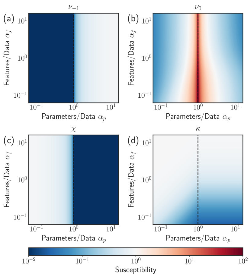
Figure 6: Susceptibilities for Random Nonlinear Features Model. Analytic solutions for three key susceptibilities as a function of $\alpha_{p}=N_{p}/M$ and $\alpha_{f}=N_{f}/M$. (a)-(b) The susceptibility $\nu$ measures the sensitivity of the fit parameters with respect to small perturbations in the gradient. In the small $\lambda$ limit, we make the approximation ${\nu\approx\lambda^{-1}\nu_{-1}+\nu_{0}}$. (a) The coefficient $\nu_{-1}$ characterizes over-parameterization, equal to the the fraction of fit parameters in excess of that needed to achieve zero training error. (b) The coefficient $\nu_{0}$ characterizes over-fitting, diverging at the interpolation threshold when $Z^{T}Z$ has a small eigenvalue. (c) The susceptibility $\chi$ measures the sensitivity of the residual label errors of the training set to small perturbations in the label noise. As a result, $\chi$ characterizes interpolation, equal to the fraction of data points that would need to be removed from the training set to achieve zero training error. (d) The susceptibility $\kappa$ measures the sensitivity of the residual parameter errors to small perturbations in the ground truth parameters. We observe that $\kappa$ decreases as a model becomes less biased, indicating that the model is better able to express the relationships underlying the data. In each panel, a black dashed line marks the boundary between the under- and over-parameterized regimes at $\alpha_{p}=1$.

V.6 Non-standard bias-variance decompositions lead to incorrect interpretations of double-descent

The analytical results for bias and variance for the random nonlinear features model extend the classical understanding of generalization into a modern setting. While the model exhibits a classical bias-variance trade-off in the under-parameterized regime, in the over-parameterized regime the test error decreases monotonically due to a monotonic reduction in both bias and variance, even in the absence of regularization. In other words, the benefits of over-parameterization are two-fold: it can reduce the likelihood of overfitting the training data, while simultaneously improving a model’s ability to capture trends hidden in the data.

The alternative and varying interpretations of the double-descent phenomenon found in previous studies are a direct result of the use of non-standard bias-variance decompositions, highlighting the importance of using the historical definitions when using these quantities to interpret double-descent. Much of this confusion can be attributed to the precise definition of what we call the sampling average in our definitions for bias and variance, which captures the randomness associated with sampling the training data $\mathcal{D}$. Previous studies have deviated from these standard definitions in two ways (see Sec. S6 of the Supporting Information sup for numerical comparisons of these alternatives with the standard definitions).

The first is the so-called fixed-design setting in which the design matrix $X$ is not included in the sampling average Adlam and Pennington (2020); Ba et al. (2020); Dereziński et al. (2020); Hastie et al. (2019); Jacot et al. (2020); Li et al. (2020); Mei and Montanari (2021). By holding the design matrix fixed for the training set, but not the test set, an effective mismatch arises between their respective data distributions, introducing an additional source of bias. As a result, one finds that the bias of the random nonlinear features model diverges at the transition, suggesting the model does not display a classical bias-variance trade-off in the under-parameterized regime, despite exhibiting a U-shaped test error Adlam and Pennington (2020); Ba et al. (2020); Mei and Montanari (2021).

In the second non-standard formulation, the random initialization of the hidden layer is included as part of the sampling average Adlam and Pennington (2020); D’Ascoli et al. (2020a, b); Jacot et al. (2020); Lin and Dobriban (2021); Yang et al. (2020). Consequently, the bias in this setting can be interpreted as measuring the bias of an ensemble model, ${\hat{y}_{\mathrm{ens}}(\vec{\mathbf{x}})=\mathrm{E}_{W}[\hat{y}(\vec{\mathbf{x}})]}$, composed of an average over all possible models with different matrices $W$, rather than the actual model under consideration. In this setting, the bias misses a contribution that would normally be incurred due to the reality that the model only utilizes a single instance of the matrix $W$, rather than averaging over the entire ensemble. In this setting, one finds that the bias of the random nonlinear features model decreases to a minimum at the interpolation threshold and then remains constant into the over-parameterized regime – paradoxically suggesting that the ability of a model to express complex relationships stops increasing once one reaches the interpolation transition Adlam and Pennington (2020); D’Ascoli et al. (2020a, b); Lin and Dobriban (2021).

In contrast to these two scenarios, we find that the bias of the nonlinear random features model monotonically decreases with the number of parameters in both the under- and over-parameterized regimes, suggesting that adding parameters while holding the number of input features fixed always increases the ability a model to capture trends in the data. This means that while there is a trade-off between bias and variance in the under-parameterized regime, this trade-off disappears in the over-parameterized regime where both bias and variance decrease as one adds fit parameters.

VI Conclusions

Understanding how the bias-variance trade-off manifests in over-parameterized models where the number of fit parameters far exceeds the number of data points is a fundamental problem in modern statistics and machine learning. Here, we have used the zero-temperature cavity method, a technique from statistical physics, to derive exact analytic expressions for the training error, test error, bias, and variance in the thermodynamic limit for two minimal model architectures: linear regression (no basis functions) and the random nonlinear features model (a two-layer neural network with nonlinear activation functions where only the top layer is trained). These analytic expressions, when combined with numerical simulations, help explain one of the most puzzling features of modern ML methods: the ability to generalize well while simultaneously achieving zero error on the training data.

We observe this phenomenon of “memorizing without overfitting” in both models. Importantly, our results show that this ability to generalize is not unique to modern ML methods such as those employed in Deep Learning; both models we consider here are convex. We also note that we do not employ commonly used methods such as stochastic gradient descent to train our models. Instead, we use a straightforward regularization procedure based on an $L_{2}$ penalty and even work in the limit where the strength of the regularization is sent to zero. This shows that the ability to generalize while achieving zero training error, sometimes referred to as interpolation, seems to be a generic property of even the simplest over-parameterized models such as linear regression and does not require any special training, regularization, or initialization methods.

Our results show that in stark contrast with the kinds of models considered in classical statistics, the variance of over-parameterized models reaches a maximum at the interpolation threshold (the model complexity at which one can achieve zero error on the training data set) and then surprisingly decreasing with model complexity beyond this threshold, giving rise to the double-descent phenomenon. These large variances at the interpolation threshold are directly tied to the existence of small eigenvalues in the Hessian matrix, which can be interpreted as a symptom of poor sampling of the data distribution by the training set when viewed by the model through the hidden features. In addition, over-parameterized models can introduce new sources of bias. Bias can arise not only from a mismatch between the model and the underlying data distribution, but also from training data sets that span only a subset of the data’s feature space. Over-parameterized models with bias can also mistake signal for noise, resulting in a nonzero variance even in the absence of noise. This shows that the properties over-parameterized models are governed by a subtle interplay between model architecture and random sampling of the data distribution via the training data set.

We note that our models are limited in two significant ways: (i) we focus on the “lazy regime” in which the kernel remains fixed during optimization and (ii) we consider convex loss landscapes containing unique solutions. In contrast, Deep Learning models in practical settings often exhibit highly non-convex loss landscapes and exist in the “feature regime” where their kernels evolve to better express the data. Many questions remain regarding the relationship between these two properties: how do neural networks learn “good” sets of features via their kernels and how do such choices relate to different local minima in the overall loss landscape? Recent work suggests that in this more complex setting, generalization error may be improved by looking for wider, more representative minima in the landscape Chaudhari et al. (2019); Baldassi et al. (2020); Pittorino et al. (2021). Understanding bias, variance, and generalization in the context of non-convex fitting functions and the relationship of these quantities to the width and local entropy of minima represents an important future area of investigation.

One possible direction for exploring these ideas may be to exploit the relationship between wide neural nets and Gaussian processes Jacot et al. (2018); Lee et al. (2019); Yaida (2020) and explore how the spectrum changes with the properties of various minima. Alternatively, one could apply our analytical approach to study fixed kernel methods in non-convex settings. For example, the perceptron exhibits a non-convex loss landscape by including negative constraint cutoffs and can be solved analytically by utilizing a Replica Symmetry Breaking ansatz Franz et al. (2017). In principle, it should be possible to extend these calculations to compute the bias-variance decomposition, eigenvalue spectrum, and susceptibilities with and without basis functions.

Finally, our analysis suggests that our conclusions may be tested directly in practical settings in two ways. First, it would be instructive to compute the eigenvalue spectra of the Hessian of Deep Learning models. It is known that the eigenvalue spectra of neural networks in the over-parameterized regime exhibit a gap with a large number of eigenvalues clustered around zero and the rest located in a nonzero bulk Sagun et al. (2018). However, there has not been a comprehensive study of how the spectrum evolves as one advances through the interpolation threshold. Second, it would be interesting to compute the relevant susceptibilities, such as those in Eq. (47). While we do not expect the susceptibilities of Deep Learning models to quantitatively match those computed here, we do expect them to follow the qualitative behavior exhibited in Fig. 6. These susceptibilities could be computed by utilizing their matrix forms (e.g., $\nu$ is the trace of the inverse Hessian), or by calculating the linear response directly via efficient differentiation techniques originally developed for computing gradients for meta-learning Finn et al. (2017). Examining such susceptibilities may also prove useful in understanding the nature of Deep Learning models in the feature regime and non-convex loss landscapes.

Appendix: Analytic Expressions for Random Nonlinear Features Model

For the random nonlinear features model, the solutions for the five averages used to express the solutions in Eqs. (18)-(21) are in turn related to a set of five scalar susceptibilities that are a natural result of the cavity method, $\nu$, $\chi$, $\kappa$, $\omega$, and $\phi$. Each of these susceptibilities is defined as the ensemble average of the trace of a different susceptibility matrix which measures the responses of quantities such as the residual label error, residual parameter error, fit parameter values, etc., to small perturbations (see Sec. V.5). Collectively, the ensemble-averaged quantities satisfy the equations

$$\expectationvalue*{\hat{w}_{1}\hat{w}_{2}} =\frac{\sigma_{\beta}^{2}}{\sigma_{W}^{2}}\frac{\sigma_{W}^{4}\frac{\alpha_{f}}{\alpha_{p}}\omega^{2}\nu^{2}}{\quantity(1-\sigma_{W}^{4}\frac{\alpha_{f}}{\alpha_{p}}\omega^{2}\nu^{2})}, \expectationvalue*{\Delta\beta_{1}\Delta\beta_{2}} =\sigma_{\beta}^{2}\frac{\kappa^{2}}{\quantity(1-\sigma_{W}^{4}\frac{\alpha_{f}}{\alpha_{p}}\omega^{2}\nu^{2})}.$$ (48)

The quantity $\expectationvalue*{\hat{u}^{2}}$ is the mean squared average of the length-$N_{f}$ vector quantity $\hat{\mathbf{u}}=X^{T}\Delta\vec{\mathbf{y}}$ obtained as a byproduct of the cavity derivation. The solutions for linear regression can be formulated similarly in terms of a pair of scalar susceptibilities that are analogous to $\chi$ and $\nu$ (see Sec. S1F of Supplemental Material sup ).

In each model, a subset of the scalar susceptibilities diverges wherever two different sets of solutions meet, indicating the existence of a second-order phase transition. For the random nonlinear features model, these susceptibilities are (to leading order in small $\lambda$)

$$\chi =\left\{\begin{array}[]{c}1-\alpha_{p}\\ \frac{\lambda}{2\sigma_{\delta z}^{2}}\frac{\alpha_{p}}{(\alpha_{p}-1)}\quantity[1-\quantity(1+\Delta\varphi)\alpha_{f}+\sqrt{\quantity[1-\quantity(1+\Delta\varphi)\alpha_{f}]^{2}+4\Delta\varphi\alpha_{f}}]\end{array}\right. \begin{array}[]{l}\mbox{\quad if\quad}N_{p}<M\\ \mbox{\quad if\quad}N_{p}>M\end{array}$$ (53)

$$\nu =\left\{\begin{array}[]{c}\frac{1}{2\sigma_{\delta z}^{2}}\frac{1}{(1-\alpha_{p})}\quantity[\alpha_{p}-\quantity(1+\Delta\varphi)\alpha_{f}+\sqrt{\quantity[\alpha_{p}-\quantity(1+\Delta\varphi)\alpha_{f}]^{2}+4\Delta\varphi\alpha_{f}\alpha_{p}}]\\ \frac{1}{\lambda}\frac{(\alpha_{p}-1)}{\alpha_{p}}++\frac{1}{2\sigma_{\delta z}^{2}}\frac{1}{(\alpha_{p}-1)}\quantity[1-\quantity(1+\Delta\varphi)\alpha_{f}+\sqrt{\quantity[1-\quantity(1+\Delta\varphi)\alpha_{f}]^{2}+4\Delta\varphi\alpha_{f}}]\end{array}\right. \begin{array}[]{l}\mbox{\quad if\quad}N_{p}<M\\ \mbox{\quad if\quad}N_{p}>M\end{array}$$ (58)

$$\kappa =\frac{1}{1+\sigma_{X}^{2}\sigma_{W}^{2}\alpha_{f}^{-1}\chi\nu}, \omega =\sigma_{X}^{2}\alpha_{f}^{-1}\chi\kappa, \phi =-\sigma_{W}^{2}\nu\kappa.$$ (59)

We plot these analytic forms for $\chi$, $\nu$ and $\kappa$ in Fig. 6.

References

- Lecun et al. (2015) Yann Lecun, Yoshua Bengio, and Geoffrey Hinton, “Deep learning,” Nature 521, 436–444 (2015).
- Canziani et al. (2017) Alfredo Canziani, Adam Paszke, and Eugenio Culurciello, “An Analysis of Deep Neural Network Models for Practical Applications,” (2017), arXiv:1605.07678 .
- Zhang et al. (2017) Chiyuan Zhang, Samy Bengio, Moritz Hardt, Benjamin Recht, and Oriol Vinyals, “Understanding Deep Learning Requires Re-thinking Generalization,” International Conference on Learning Representations (ICLR) (2017).
- Mehta et al. (2019a) Pankaj Mehta, Marin Bukov, Ching Hao Wang, Alexandre G.R. Day, Clint Richardson, Charles K. Fisher, and David J. Schwab, “A high-bias, low-variance introduction to Machine Learning for physicists,” Physics Reports 810, 1–124 (2019a).
- (5) “See supplemental material at [url] for complete analytic derivations and additional numerical results.” .
- Belkin et al. (2019) Mikhail Belkin, Daniel Hsu, Siyuan Ma, and Soumik Mandal, “Reconciling modern machine-learning practice and the classical bias–variance trade-off,” Proceedings of the National Academy of Sciences 116, 15849–15854 (2019).
- Geiger et al. (2019) Mario Geiger, Stefano Spigler, Stéphane D’Ascoli, Levent Sagun, Marco Baity-Jesi, Giulio Biroli, and Matthieu Wyart, “Jamming transition as a paradigm to understand the loss landscape of deep neural networks,” Physical Review E 100, 012115 (2019).
- Spigler et al. (2019) S. Spigler, M. Geiger, S D’Ascoli, L. Sagun, G. Biroli, and M. Wyart, “A jamming transition from under- to over-parametrization affects generalization in deep learning,” Journal of Physics A: Mathematical and Theoretical 52, 474001 (2019).
- Mailman and Chakraborty (2011) M Mailman and B Chakraborty, “A signature of a thermodynamic phase transition in jammed granular packings: growing correlations in force space,” Journal of Statistical Mechanics: Theory and Experiment 2011, L07002 (2011).
- Bahri et al. (2020) Yasaman Bahri, Jonathan Kadmon, Jeffrey Pennington, Sam S. Schoenholz, Jascha Sohl-Dickstein, and Surya Ganguli, “Statistical Mechanics of Deep Learning,” Annual Review of Condensed Matter Physics 11, 501–528 (2020).
- Kobak [@hippopedoid] (2020) Dmitry Kobak [@hippopedoid], “Twitter Thread: twitter.com/hippopedoid/status/1243229021921579010,” (2020).
- Loog et al. (2020) Marco Loog, Tom Viering, Alexander Mey, Jesse H. Krijthe, and David M. J. Tax, “A brief prehistory of double descent,” Proceedings of the National Academy of Sciences 117, 10625–10626 (2020).
- Nakkiran et al. (2020) Preetum Nakkiran, Gal Kaplun, Yamini Bansal, Tristan Yang, Boaz Barak, and Ilya Sutskever, “Deep Double Descent: Where Bigger Models and More Data Hurt,” International Conference on Learning Representations (ICLR) (2020).
- Jacot et al. (2018) Arthur Jacot, Franck Gabriel, and Clément Hongler, “Neural tangent kernel: Convergence and generalization in neural networks,” Advances in Neural Information Processing Systems (NeurIPS) 31 (2018).
- Lee et al. (2019) Jaehoon Lee, Lechao Xiao, Samuel S. Schoenholz, Yasaman Bahri Roman Novak, Jascha Sohl-Dickstein, and Jeffrey Pennington, “Wide neural networks of any depth evolve as linear models under gradient descent,” Advances in Neural Information Processing Systems (NeurIPS) 32 (2019).
- Geiger et al. (2020) Mario Geiger, Stefano Spigler, Arthur Jacot, and Matthieu Wyart, “Disentangling feature and lazy training in deep neural networks,” Journal of Statistical Mechanics: Theory and Experiment 2020, 113301 (2020).
- Adlam and Pennington (2020) Ben Adlam and Jeffrey Pennington, “Understanding double descent requires a fine-grained bias-variance decomposition,” Advances in Neural Information Processing Systems (NeurIPS) 33, 11022–11032 (2020).
- Advani et al. (2020) Madhu S. Advani, Andrew M. Saxe, and Haim Sompolinsky, “High-dimensional dynamics of generalization error in neural networks,” Neural Networks 132, 428–446 (2020).
- Ba et al. (2020) Jimmy Ba, Murat Erdogdu, Taiji Suzuki, Denny Wu, and Tianzong Zhang, “Generalization of Two-layer Neural Networks: An Asymptotic Viewpoint,” International Conference on Learning Representations (ICLR) (2020).
- Barbier et al. (2019) Jean Barbier, Florent Krzakala, Nicolas Macris, Léo Miolane, and Lenka Zdeborová, “Optimal errors and phase transitions in high-dimensional generalized linear models,” Proceedings of the National Academy of Sciences 116, 5451–5460 (2019).
- Bartlett et al. (2020) Peter L. Bartlett, Philip M. Long, Gábor Lugosi, and Alexander Tsigler, “Benign overfitting in linear regression,” Proceedings of the National Academy of Sciences 117, 30063–30070 (2020).
- Belkin et al. (2020) Mikhail Belkin, Daniel Hsu, and Ji Xu, “Two Models of Double Descent for Weak Features,” SIAM Journal on Mathematics of Data Science 2, 1167–1180 (2020).
- Bibas et al. (2019) Koby Bibas, Yaniv Fogel, and Meir Feder, “A New Look at an Old Problem: A Universal Learning Approach to Linear Regression,” IEEE International Symposium on Information Theory (ISIT) , 2304–2308 (2019).
- Deng et al. (2020) Zeyu Deng, Abla Kammoun, and Christos Thrampoulidis, “A Model of Double Descent for High-Dimensional Logistic Regression,” IEEE International Conference on Acoustics, Speech and Signal Processing (ICASSP) , 4267–4271 (2020).
- D’Ascoli et al. (2020a) Stéphane D’Ascoli, Levent Sagun, and Giulio Biroli, “Triple descent and the two kinds of overfitting: Where & why do they appear?” Advances in Neural Information Processing Systems (NeurIPS) 33 (2020a).
- D’Ascoli et al. (2020b) Stéphane D’Ascoli, Maria Refinetti, Giulio Biroli, and Florent Krzakala, “Double Trouble in Double Descent: Bias and Variance(s) in the Lazy Regime,” Proceedings of the 37th International Conference on Machine Learning (ICML) PMLR, 119, 2280–2290 (2020b).
- Dereziński et al. (2020) Michał Dereziński, Feynman Liang, and Michael W. Mahoney, “Exact expressions for double descent and implicit regularization via surrogate random design,” Advances in Neural Information Processing Systems (NeurIPS) 33, 5152–5164 (2020).
- Dhifallah and Lu (2020) Oussama Dhifallah and Yue M. Lu, “A Precise Performance Analysis of Learning with Random Features,” (2020), arXiv:2008.11904 .
- Gerace et al. (2020) Federica Gerace, Bruno Loureiro, Florent Krzakala, Marc Mézard, and Lenka Zdeborová, “Generalisation error in learning with random features and the hidden manifold model,” Proceedings of the 37th International Conference on Machine Learning (ICML) PMLR, 119, 3452–3462 (2020).
- Hastie et al. (2019) Trevor Hastie, Andrea Montanari, Saharon Rosset, and Ryan J. Tibshirani, “Surprises in High-Dimensional Ridgeless Least Squares Interpolation,” (2019), arXiv:1903.08560 .
- Jacot et al. (2020) Arthur Jacot, Berfin Şimşek, Francesco Spadaro, Clément Hongler, and Franck Gabriel, “Implicit regularization of random feature models,” Proceedings of the 37th International Conference on Machine Learning (ICML) PMLR, 119, 4631–4640 (2020).
- Kini and Thrampoulidis (2020) Ganesh Ramachandra Kini and Christos Thrampoulidis, “Analytic Study of Double Descent in Binary Classification: The Impact of Loss,” IEEE International Symposium on Information Theory (ISIT) , 2527–2532 (2020).
- Lampinen and Ganguli (2019) Andrew K. Lampinen and Surya Ganguli, “An analytic theory of generalization dynamics and transfer learning in deep linear networks,” International Conference on Learning Representations (ICLR) (2019).
- Li et al. (2020) Zhu Li, Weijie J. Su, and Dino Sejdinovic, “Benign overfitting and noisy features,” (2020), arXiv:2008.02901 .
- Liang and Rakhlin (2020) Tengyuan Liang and Alexander Rakhlin, “Just interpolate: Kernel “Ridgeless” regression can generalize,” Annals of Statistics 48, 1329–1347 (2020).
- Liang et al. (2020) Tengyuan Liang, Alexander Rakhlin, and Xiyu Zhai, “On the Multiple Descent of Minimum-Norm Interpolants and Restricted Lower Isometry of Kernels,” Proceedings of Thirty Third Conference on Learning Theory PMLR, 125, 2683–2711 (2020).
- Liao et al. (2020) Zhenyu Liao, Romain Couillet, and Michael W Mahoney, “A random matrix analysis of random Fourier features: beyond the Gaussian kernel, a precise phase transition, and the corresponding double descent,” Advances in Neural Information Processing Systems (NeurIPS) 33 (2020).
- Lin and Dobriban (2021) Licong Lin and Edgar Dobriban, “What causes the test error? Going beyond bias-variance via ANOVA,” Journal of Machine Learning Research 22, 1–82 (2021).
- Mitra (2019) Partha P Mitra, “Understanding overfitting peaks in generalization error: Analytical risk curves for and penalized interpolation,” (2019), arXiv:1906.03667 .
- Mei and Montanari (2021) Song Mei and Andrea Montanari, “The Generalization Error of Random Features Regression: Precise Asymptotics and the Double Descent Curve,” Communications on Pure and Applied Mathematics (2021), 10.1002/cpa.22008.
- Muthukumar et al. (2019) Vidya Muthukumar, Kailas Vodrahalli, and Anant Sahai, “Harmless interpolation of noisy data in regression,” IEEE International Symposium on Information Theory (ISIT) , 2299–2303 (2019).
- Nakkiran (2019) Preetum Nakkiran, “More Data Can Hurt for Linear Regression: Sample-wise Double Descent,” (2019), arXiv:1912.07242 .
- Xu and Hsu (2019) Ji Xu and Daniel Hsu, “On the number of variables to use in principal component regression,” Advances in Neural Information Processing Systems (NeurIPS) 32 (2019).
- Yang et al. (2020) Zitong Yang, Yaodong Yu, Chong You, Jacob Steinhardt, and Yi Ma, “Rethinking Bias-Variance Trade-off for Generalization of Neural Networks,” Proceedings of the 37th International Conference on Machine Learning (ICML) PMLR, 119, 10767–10777 (2020).
- Dauphin et al. (2014) Yann N. Dauphin, Razvan Pascanu, Caglar Gulcehre, Kyunghyun Cho, Surya Ganguli, and Yoshua Bengio, “Identifying and attacking the saddle point problem in high-dimensional non-convex optimization,” Advances in Neural Information Processing Systems (NeurIPS) 27 (2014).
- Engel et al. (2001) A Engel, C den Broeck, and C Broeck, Statistical Mechanics of Learning, Statistical Mechanics of Learning (Cambridge University Press, 2001).
- Mézard and Parisi (2003) Marc Mézard and Giorgio Parisi, “The Cavity Method at Zero Temperature,” Journal of Statistical Physics 111, 1–34 (2003).
- Ramezanali et al. (2015) Mohammad Ramezanali, Partha P. Mitra, and Anirvan M. Sengupta, “The cavity method for analysis of large-scale penalized regression,” (2015), arXiv:1501.03194 .
- Mehta et al. (2019b) Pankaj Mehta, Wenping Cui, Ching-Hao Wang, and Robert Marsland, “Constrained optimization as ecological dynamics with applications to random quadratic programming in high dimensions,” Physical Review E 99, 052111 (2019b).
- Advani et al. (2018) Madhu Advani, Guy Bunin, and Pankaj Mehta, “Statistical physics of community ecology: a cavity solution to MacArthur’s consumer resource model,” Journal of Statistical Mechanics: Theory and Experiment 2018, 033406 (2018).
- Marčenko and Pastur (1967) Vladimir Alexandrovich Marčenko and Leonid Andreevich Pastur, “Distribution of eigenvalues for some sets of random matrices,” Mathematics of the USSR-Sbornik 1, 457–483 (1967).
- Pennington and Worah (2019) Jeffrey Pennington and Pratik Worah, “Nonlinear random matrix theory for deep learning,” Journal of Statistical Mechanics: Theory and Experiment 2019, 124005 (2019).
- Mézard (2017) Marc Mézard, “Mean-field message-passing equations in the Hopfield model and its generalizations,” Physical Review E 95, 022117 (2017).
- Ramezanali et al. (2019) Mohammad Ramezanali, Partha P. Mitra, and Anirvan M. Sengupta, “Critical Behavior and Universality Classes for an Algorithmic Phase Transition in Sparse Reconstruction,” Journal of Statistical Physics 175, 764–788 (2019).
- Cui et al. (2020) Wenping Cui, Jason W. Rocks, and Pankaj Mehta, “The perturbative resolvent method: Spectral densities of random matrix ensembles via perturbation theory,” (2020), arXiv:2012.00663 .
- Bishop (2006) Christopher M. Bishop, Pattern Recognition and Machine Learning (Springer, 2006).
- Goldt et al. (2020) Sebastian Goldt, Marc Mézard, Florent Krzakala, and Lenka Zdeborová, “Modeling the Influence of Data Structure on Learning in Neural Networks: The Hidden Manifold Model,” Physical Review X 10, 041044 (2020).
- Rocks and Mehta (2021) Jason W. Rocks and Pankaj Mehta, “The Geometry of Over-parameterized Regression and Adversarial Perturbations,” (2021), arXiv:2103.14108 .
- Chaudhari et al. (2019) Pratik Chaudhari, Anna Choromanska, Stefano Soatto, Yann LeCun, Carlo Baldassi, Christian Borgs, Jennifer Chayes, Levent Sagun, and Riccardo Zecchina, “Entropy-SGD: biasing gradient descent into wide valleys,” Journal of Statistical Mechanics: Theory and Experiment 2019, 124018 (2019).
- Baldassi et al. (2020) Carlo Baldassi, Enrico M. Malatesta, Matteo Negri, and Riccardo Zecchina, “Wide flat minima and optimal generalization in classifying high-dimensional Gaussian mixtures,” Journal of Statistical Mechanics: Theory and Experiment 2020, 124012 (2020).
- Pittorino et al. (2021) Fabrizio Pittorino, Carlo Lucibello, Christoph Feinauer, Enrico M. Malatesta, Gabriele Perugini, Carlo Baldassi, Matteo Negri, Elizaveta Demyanenko, and Riccardo Zecchina, “Entropic gradient descent algorithms and wide flat minima,” International Conference on Learning Representations (ICLR) (2021).
- Yaida (2020) Sho Yaida, “Non-Gaussian processes and neural networks at finite widths,” Proceedings of The First Mathematical and Scientific Machine Learning Conference PMLR, 107, 165–192 (2020).
- Franz et al. (2017) Silvio Franz, Giorgio Parisi, Maksim Sevelev, Pierfrancesco Urbani, and Francesco Zamponi, “Universality of the SAT-UNSAT (jamming) threshold in non-convex continuous constraint satisfaction problems,” SciPost Physics 2, 019 (2017).
- Sagun et al. (2018) Levent Sagun, Utku Evci, V. U˘gur Güney, Yann Dauphin, and Léon Bottou, “Empirical analysis of the hessian of over-parametrized neural networks,” (2018), arXiv:1706.04454 .
- Finn et al. (2017) Chelsea Finn, Pieter Abbeel, and Sergey Levine, “Model-agnostic meta-learning for fast adaptation of deep networks,” Proceedings of the 34th International Conference on Machine Learning (ICML) PMLR, 70, 1126—-1135 (2017).