Probing Oscillons of Ultra-Light Axion-like Particle by 21cm Forest

Abstract

Ultra-Light Axion-like Particle (ULAP) is motivated as one of the solutions to the small scale problems in astrophysics. When such a scalar particle oscillates with an $\mathcal{O}(1)$ amplitude in a potential shallower than quadratic, it can form a localized dense object, oscillon. Because of its longevity due to the approximate conservation of the adiabatic invariant, it can survive up to the recent universe as redshift $z\sim\mathcal{O}(10)$. The scale affected by these oscillons is determined by the ULAP mass $m$ and detectable by observations of 21cm line. In this paper, we examine the possibility to detect ULAP by 21cm line and find that the oscillon can enhance the signals of 21cm line observations when $m\lesssim 10^{-19}\ {\rm eV}$ and the fraction of ULAP to dark matter is much larger than $10^{-2}$ depending on the form of the potential.

1 Introduction

The nature of dark matter that dominates the matter energy density of the universe remains a huge mystery, though various observational results suggest its existence [1, 2, 3]. Thanks to the relentless efforts for cosmological observations over the past decades, particularly the observations of cosmic microwave background (CMB), cosmological constant and cold dark matter ($\Lambda$CDM) model with inflation is revealed to be the most promising [4, 5, 6] among many cosmological models on large scales.

However, looking into the small scales around $\lesssim 1{\rm Mpc}$, numerical simulations based on the $\Lambda$CDM model confronts three astrophysical problems, missing satellite problem (e.g. [7]), core cusp problem (e.g. [8]), and too big to fail problem (e.g. [9]) (see also Ref. [10] for a review). Because all these problems arise from the over-density at small scales, scientists are struggling to construct the dark matter model that suppresses the small scale structure while behaves like cold dark matter at large scales.

Ultra-Light Axion-like Particle (ULAP) originated from the spontaneous symmetry breaking of string theory [11] is one of the fascinating particles that can solve such small scale problems. For example, considering the mass with $m\simeq 10^{-22}\ {\rm eV}$, the de Broglie wavelength of ULAP is about $\sim$ kpc which is the typical scale of the galactic center. Smoothing out the central over density by the quantum pressure, the core cusp problem can be solved [12, 13].

Generally, ULAP is assumed to be coherently oscillating around the universe. However, there is a possibility that this scalar particle exists in the form of a localized dense object, oscillon [14, 15, 16] (See [17, 18, 19] for earlier study of the formation.). The necessary condition for oscillon formation is just the potential shallower than quadratic. The lifetime of oscillons is estimated as

$$\tau\sim 2\ {\rm Gyr}\left(\frac{10^{-22}\ {\rm eV}}{m}\right)\left(\frac{\Gamma/m}{10^{-10}}\right)^{-1}.$$ (1.1)

where $\Gamma$ is the decay rate of the oscillon which can be analytically calculated [20, 21]. Thus, if $\Gamma/m\lesssim 10^{-11}$, the produced oscillons can exist even in the current universe. The lifetime of oscillon is quite long in general because of the approximate conservation of the adiabatic charge [22, 23, 24] while it also depends on the shape of the potential. In the pure natural type potential, for example, it is proved that the resultant oscillons are quite long-lived [25, 26]. In this case, we can take advantage of the high density of oscillons to detect the clue to ULAP.

The oscillon formation affects fluctuations with comoving scale $m/\sqrt{10}\lesssim k/a\lesssim m$, that is,

$$15\ {\rm Mpc^{-1}}\left(\frac{m}{10^{-22}\ {\rm eV}}\right)^{1/2}\lesssim k\lesssim 50\ {\rm Mpc^{-1}}\left(\frac{m}{10^{-22}\ {\rm eV}}\right)^{1/2},$$ (1.2)

where the upper bound is roughly determined by the typical distance between oscillons, and the lower bound is by the horizon scale at oscillon formation. This is because the typical oscillon distance is the same as the wavenumber of the parametric resonance $\sim m$, and oscillons are generally produced when the scale factor $a$ becomes $\mathcal{O}(10)$ times larger than the initial value determined by the condition $H\simeq m$.

One of the methods to explore this scale is the 21cm line, which is produced by the hyperfine splitting by the interaction between the electron and proton spins [27]. Generally, the 21cm line is adopted as the useful tracer of the recent billion years of the universe because neutral hydrogen is ubiquitous in the early universe after the recombination, amounting to $\sim 75$% of the gas present in the intergalactic medium (IGM).

If there are luminous radio rich sources such as radio quasars and gamma-ray bursts (GRBs), the emitted continuum spectrum is consecutively absorbed by the neutral hydrogen; this absorption mechanism is called 21cm forest [28, 29] in analogy to the Lyman-$\alpha$ forest. The absorption could be the most efficient when the emission spectrum goes through the neutral hydrogen-rich region. Such regions during the epoch of reionization and beyond are called mini-halos characterized by the virial temperature smaller than $10^{4}\ {\rm K}$ [30]. Because under this temperature the metal-free cooling necessary for the star formation becomes ineffective and the amount of resultant X-rays is reduced, plenty of neutral hydrogen remains in mini-halos.

In this paper, we focus on the detection of ULAP by 21cm forest when some or all of ULAP is in the form of oscillon. In the previous researches [31, 32], the contribution of ULAP to the 21cm forest is discussed, but the possibility of ULAP oscillon formation has never been considered. Here, we assume that dark matter of the universe is consist of unknown cold dark matter, homogeneous ULAP, and ULAP oscillons,

$$\Omega_{{\rm DM}} =\Omega_{{\rm CDM}}+\Omega_{{\rm ULAP}},$$ (1.3)

$$=\Omega_{{\rm CDM}}+\left(\Omega_{{\rm homo}}+\Omega_{{\rm osc}}\right).$$ (1.4)

For later use, we define the fraction of ULAP to cold dark matter $f_{{\rm ULAP}}$ as

$$\Omega_{{\rm ULAP}}\equiv f_{{\rm ULAP}}\Omega_{{\rm DM}}.$$ (1.5)

The organization of this paper is as follows. In Sec. 2, we analytically derive the matter power spectrum under the situation where the ULAP oscillons are present in the universe following Ref. [33]. In Sec. 3, we calculate the abundance of the 21cm absorption lines. Finally, in Sec. 4 and Sec. 5 we discuss and conclude the result. All cosmological parameters in this paper are extracted from the result of Planck 2018 [6].

2 Matter Power Spectrum

In this section, we briefly explain the matter power spectrum of the dark matter consist of unknown cold dark matter, homogeneous ULAP, and ULAP oscillons following Ref. [33]. The details of the derivation are written in Appendix A and Ref. [33].

The matter power spectrum $P(k)$ is decomposed as

$$P(k,t) =P_{{\rm CDM}}(k,t)+P_{{\rm ULAP}}(k,t),$$ (2.1)

$$=P_{{\rm CDM}}(k,t)+\left[P_{{\rm homo}}(k,t)+P_{{\rm osc}}(k,t)\right].$$ (2.2)

where $P_{{\rm homo}}(k,t)$ and $P_{{\rm osc}}(k,t)$ show the matter power spectra of homogeneous ULAP and ULAP oscillons, respectively and we assumed that the homogeneous part and the oscillon part are not correlated. We calculate $P_{{\rm{\rm CDM}}}(k,t)+P_{{\rm homo}}(k,t)$ from the AxionCAMB code [34] which is originated from the public Boltzmann code CAMB [35, 36]. Because homogeneous ULAP suppresses the small scale structure, the matter power spectrum is also suppressed as $P_{\rm CDM}+P_{\rm homo}<P_{\Lambda{\rm CDM}}$, which generally reduces the number of 21cm absoptions.

2.1 ULAP Model

As the ULAP potential, we choose the monodromy type potential [37, 38, 39]

$$V(\phi)=\frac{m^{2}F^{2}}{2p}\left[1-\left(1+\frac{\phi^{2}}{F^{2}}\right)^{-p}\right].$$ (2.3)

When $p>-1$, the oscillon formation is confirmed in Ref. [26]. It is also confirmed both analytically and numerically that the produced oscillons live very long [25, 20, 21]. In this paper, we take $p=-3/4$, for instance.

2.2 Oscillon Matter Power Spectrum

The analytical formula of the oscillon power spectrum has been developed in Ref [33] when the positions of produced oscillons are not correlated. See Ref. [33] and Appendix A for details of the derivation. Defining the energy ratio of oscillons to ULAP $r_{\rm osc}(t)$ as

$$r_{\rm osc}(t)\equiv\frac{\Omega_{\rm osc}}{\Omega_{\rm ULAP}},$$ (2.4)

and neglecting the oscillon size ($k/a\ll m$), the power spectrum at the oscillon formation time $t_{f}$ is written as

$$P_{\rm osc}\left(k,t_{f}\right)=\frac{\left(r_{\rm osc}(t)f_{\rm ULAP}\right)^{2}}{n_{\rm osc}a^{3}}\left(\frac{\Omega_{\rm DM}}{\Omega_{m}}\right)^{2}\frac{\langle M_{\rm osc}^{2}\rangle}{\langle M_{\rm osc}\rangle^{2}}\left[1-\left(\frac{2}{kL_{s}}\right)^{2}\sin^{2}\frac{kL_{s}}{2}\right],$$ (2.5)

where the bracket $\langle\rangle$ represents the ensemble average over oscillons, $M_{\rm osc}$ is the total energy of a oscillon, and $n_{\rm osc}$ is the physical number density of oscillons. $P_{\rm osc}$ is obtained by multiplying the Poisson power spectrum $1/(n_{\text{osc}}a^{3})$ by the energy fraction of oscillons, the squared average of the oscillon mass $\langle M_{\rm osc}^{2}\rangle/\langle M_{\rm osc}\rangle^{2}$, and a suppression term. The suppression is effective on scales larger than the horizon at the oscillon formation due to energy conservation. Eq. (2.5) includes this suppression factor with $L_{s}$ being the cut-off scale [33].

Taking into account the time evolution after the oscillon formation, this power spectrum is affected by two effects: the partial decay of the oscillons and the gravitational growth of the isocurvature fluctuations.

First, let us consider the decay process of the produced oscillons. Because oscillons are getting smaller by emitting the self-radiation, the oscillon distribution also evolves. Following Refs. [20, 21], we can analytically calculate the oscillon decay rate $\Gamma$

$$\Gamma\equiv\frac{1}{M_{\rm osc}}\left|\frac{dM_{\rm osc}}{dt}\right|.$$ (2.6)

as shown in Fig. 1.

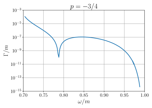
Figure 1: The decay rate of the oscillon for $p=-3/4$. The horizontal axis $\omega$ shows the oscillation frequency of the scalar field.

Using this decay rate, we can evolve the oscillon distribution from the formation time. The simulation result and the evolved distributions are shown in Fig 2. Please see Appendix B for the details of the simulation.

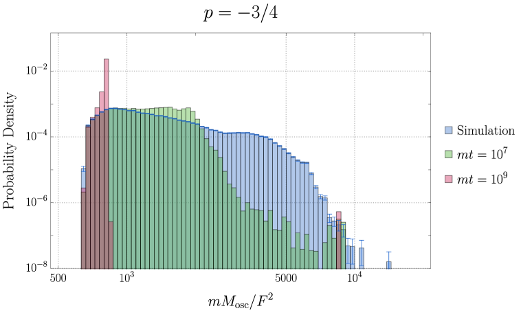
Figure 2: The probability density of the oscillon mass distribution derived from the lattice simulation which contains $\sim 10^{5}$ oscillons. The horizontal axis is normalized by the ULAP mass $m$ and the decay constant of ULAP $F$. The yellow region shows the oscillon distribution at the formation time, and the blue and green region show the distribution at $mt=10^{7}$ and $mt=10^{9}$, respectively. The width of the $i$-th bin is $\Delta x_{i}\equiv 10^{14/5}\left(10^{(i+1)/50}-10^{i/50}\right)$ and statistical error of the simulation result is given by $\sqrt{N_{i}}/(N_{\rm osc}\Delta x_{i})$ where $N_{i}$ is the number of data in the $i$-th bin and $N_{\rm osc}$ is the total number of data.

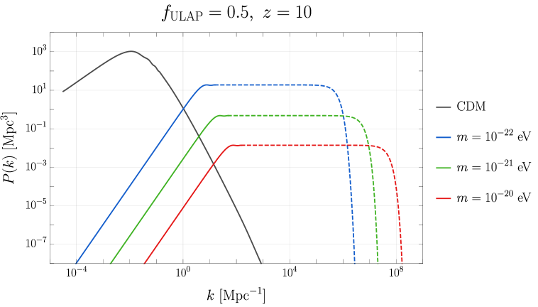
Figure 3: The matter power spectrum of oscillons when $f_{\rm ULAP}=0.5$ at $z=10$. The blue, green, and red lines show the oscillon matter power spectrum of $m=10^{-22}\ {\rm eV},\ m=10^{-21}\ {\rm eV},$ and $m=10^{-20}\ {\rm eV}$ respectively. We truncated the matter power spectrum at the point where the oscillon number equals to $10$ because the fluctuation of a single oscillon is non-linear. These regions are plotted as dashed lines. Note that the exponential cutoff on the right side of the figure $k/a\sim m$ is because of the radius of a oscillon [33]. We also plotted the matter power spectrum of $\Lambda$CDM model as the black line for comparison.

The second is the growth of the fluctuations in the radiation and matter dominated era. In the parameter region of ULAP mass $m\gtrsim 10^{-28}\ {\rm eV}$ where we are interested, oscillons are produced in the radiation dominated era. The fluctuations linearly grow after the matter-radiation equality and the oscillon power spectrum in the matter dominated era ($t>t_{{\rm eq}}$) is

$$P_{\rm osc}(k,t)=\left(\frac{3}{2}\frac{a}{a_{{\rm eq}}}\right)^{2}P_{\rm osc}(k,t_{f}).$$ (2.7)

where $a_{\rm eq}\simeq 1/3400$ is the scale factor at the matter-radiation equality.

Considering these two effects, the oscillon matter power spectrum at $z=10$ is calculated as shown in Fig. 3. In the figure, we also take into account the non-linearity of the energy density of oscillons. The linear matter power spectrum must be truncated at least below the scale where the oscillon number is smaller than $2$ because the fluctuation is non-linear in that scale. Thus, we cut off the power spectrum on the scale $k_{\rm cut}$ where the number of oscillons equals to $10$ as $n_{\rm osc}(2\pi/k_{\rm cut})^{3}=10$, for instance. These lines are shown as dotted lines in Fig. 3.

3 Abundance of 21cm Absorption Lines

In this section, we calculate the abundance of 21cm absorption lines when mini-halos contains ULAP oscillons. The procedure of this section follows Refs. [29, 40, 31, 32].

3.1 Mini-Halo Profile

To calculate the 21cm line absorption abundance, it is important to estimate the abundance of the neutral hydrogen which absorbs the photon of background light sources. In this subsection, we propose a decent assumption of the matter distribution inside halos to derive the neutral hydrogen distribution.

3.1.1 Dark Matter Halo Profile

The dark matter halo profile at the low redshift is well described by the Navarro, Frenk, and White (NFW) profile [41, 42],

$$\rho_{DM}(r)=\frac{\rho_{DM0}}{r/r_{s}\left(1+r/r_{s}\right)^{2}}\equiv\frac{\rho_{DM0}}{xy\left(1+xy\right)^{2}}.$$ (3.1)

where $r_{s}$ is the scale papameter, $x,y$ are defined as $x\equiv r/r_{\rm vir},\ y\equiv r_{\rm vir}/r_{s}$, and $r_{\rm vir}$ is the virial radius. $y$ is often called the concentration paramter and fitted in Ref. [43] as

$$y=\frac{14.8}{1+z}\left(\frac{M}{1.3\times 10^{13}h^{-1}M_{\odot}}\right)^{-0.14},$$ (3.2)

where we set $M$ as the virial mass, $M_{\odot}=1.33\times 10^{33}\ {\rm kg}$ is the solar mass, and $h=0.68$ is the normalized Hubble parameter.

The virial radius $r_{\rm vir}$ is calculated by the spherical collapse model [45], which derives

$$r_{\rm vir} =\left(\frac{M}{\frac{4\pi}{3}\rho_{m}(z)\Delta}\right)^{1/3},$$ (3.3)

$$=0.53\ {\rm kpc}\left(\frac{M}{10^{8}h^{-1}M_{\odot}}\right)^{1/3}\left(\frac{\Omega_{m0}}{\Omega_{m}}\frac{\Delta}{18\pi^{2}}\right)^{-1/3}\left(\frac{1+z}{10}\right)^{-1}.$$ (3.4)

where $\Delta\equiv 18\pi^{2}+82d-39d^{2}$, and $d\equiv\Omega_{m}(z)-1$. $\rho_{m}(z)$ is the matter energy density at the redshift $z$ and $\Omega_{m}(z)=\rho_{m}(z)/\rho_{c}(z)$ where $\rho_{c}(z)$ is the critical energy density at the redshift $z$. From the above relations, the central energy density $\rho_{DM0}$ is determined as

$$\rho_{DM0}=\frac{M}{\int_{0}^{r_{\rm vir}}\left[r/r_{s}\left(1+r/r_{s}\right)^{2}\right]^{-1}d^{3}r}.$$ (3.5)

3.1.2 Gas Profile

For simplicity, we make two assumptions on the gas within halos.

• Isothermal: The gas within halos is isothermal because it is virialized. Defining the virial temperature as $\langle K\rangle=(3/2)k_{B}T_{\rm vir}$ where $\langle K\rangle$ is the time-averaged kinetic energy per particle of the system, the virial theorem leads to

  $$T_{\rm vir}\simeq\frac{\mu}{2k_{B}}\frac{GM}{r_{\rm vir}}.$$ (3.6)

  Here $k_{B}$ is the Boltzmann constant and $\mu=1.22m_{p}$ is the mean molecular weight of the gas [30].

• In hydrostatic equilibrium: At the distance $r$ from the origin, the gas pressure $P(r)$ and the gravitational force are balanced [46].

  $$\frac{dP(r)}{dr}=-\frac{GM(r)}{r^{2}}\rho_{g}(r),$$ (3.7)

  where $\rho_{g}(r)$ shows the gas profile. The gas pressure is easily calculated from the equation of state as

  $$P(r)=\frac{\rho_{g}(r)}{\mu}k_{B}T_{\rm vir}.$$ (3.8)

  From the above two assumptions, the gas profile $\rho_{g}(r)$ is

  $$\rho_{g}(r)=\rho_{g0}\exp\left[-\frac{\mu}{2k_{B}T_{\rm vir}}\left(v_{{\rm esc}}(0)^{2}-v_{{\rm esc}}(r)^{2}\right)\right],$$ (3.9)

  where

  $$v_{{\rm esc}}(r)^{2}=2\int_{r}^{\infty}\frac{GM(\tilde{r})}{\tilde{r}^{2}}d\tilde{r}=\frac{2GM}{r_{\rm vir}}\frac{\log(1+xy)}{x\left[\log(1+y)-\frac{y}{1+y}\right]}.$$ (3.10)

The normalization of the gas profile $\rho_{g0}$ is determined by the ratio of the baryon energy density $\Omega_{b}$ and matter energy density $\Omega_{m}$ as

$$\frac{M_{g}}{M}=\frac{\Omega_{b}}{\Omega_{m}},\quad\Leftrightarrow\quad\rho_{g0}=\frac{\Delta}{3}\frac{y^{3}e^{A}}{\int_{0}^{y}(1+t)^{A/t}t^{2}dt}\frac{\Omega_{b}}{\Omega_{m}}\rho_{m}(z),$$ (3.11)

where

$$A\equiv\frac{3y}{\log(1+y)-y/(1+y)}.$$ (3.12)

From all above calculations, the number deinsty profile of the neutral hydrogen is derived as

$$n_{HI}(r)=0.74\times\frac{\rho_{g}(r)}{m_{p}}.$$ (3.13)

3.2 Halo Mass Function

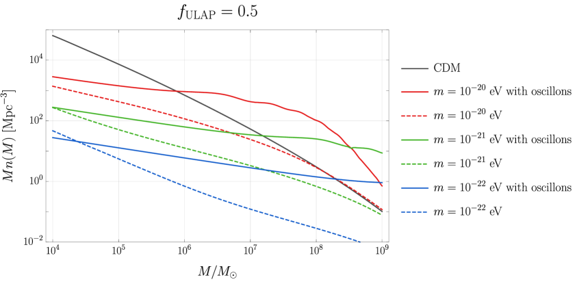
Figure 4: The halo-mass function when $f_{\rm ULAP}=0.5$. The red, green, and blue lines show the result of $m=10^{-20}\ {\rm eV},\ m=10^{-21}\ {\rm eV},$ and $m=10^{-22}\ {\rm eV}$. The solid and dashed lines show the halo mass function with ULAP oscillons and without ULAP oscillon respectively. We also plotted the halo-mass function of $\Lambda$CDM model as the black line for comparison.

In this paper, we use the Press-Schechter formalism [47] to calculate the halo-mass function. Although the Sheth-Tormen mass function [48] is more precise in a low redshift, the situation is currently unclear for $z\sim 10$. Thus, we use the Press-Schechter formalism in this work and review it below.

First, we define the coarse-grained fluctuation as

$$\delta_{{\rm cg}}(\bm{x},R)\equiv\int d^{3}x\delta(\bm{x})W(\bm{x},R),$$ (3.14)

where we use the real space top-hat function as the window function $W(\bm{x},R)$ in this paper. Assuming that the energy density fraction follows the Gaussian distribution, the probability that we can find the over-dense region where $\delta_{{\rm cg}}>\delta_{c}\simeq 1.686$ in the linear perturbation theory is

$$P(>\delta_{c})=\frac{1}{\sqrt{2\pi}\sigma(R)}\int_{\delta_{c}}^{\infty}\exp\left(-\frac{\delta_{{\rm cg}}^{2}}{2\sigma(R)^{2}}\right)d\delta_{cg},$$ (3.15)

where $\sigma(R)$ is the coarse-grained variance and

$$\sigma(R)^{2} \equiv\langle\delta_{cg}^{2}(\bm{x},R)\rangle=\int P(k)\left|W(kR)\right|^{2}d^{3}k.$$ (3.16)

We substitute the matter power spectrum derived in Sec. 2 for $P(k)$. Because the coarse-grained comoving radius $R$ is related to the halo mass $M$ as

$$M=\frac{4\pi R^{3}}{3}\rho_{m0},$$ (3.17)

we can take $\sigma$ as the function of $M$ instead of $R$. Then, the comoving number density of halos with the mass $M$ is calculated from the Press-Schechter formalism as

$$n(M,z)dM =2\frac{\rho_{m0}}{M}\frac{\partial P(>\delta_{c})}{\partial M}dM,$$ (3.18)

$$=\sqrt{\frac{2}{\pi}}\frac{\rho_{m0}}{M}\frac{\delta_{c}}{\sigma(M)^{2}}\exp\left(-\frac{\delta_{c}^{2}}{2\sigma(M)^{2}}\right)\left|\frac{\partial\sigma(M)}{\partial M}\right|dM.$$ (3.19)

The calculation results are shown in Fig. 4. When ULAP without oscillons exists as dark matter, the number of halos is suppressed compared to the CDM case because of the quantum pressure of ULAP as shown in dashed lines. On the other hand, the solid lines which exhibit the halo-mass function with ULAP oscillons are always larger than the corresponding dashed lines, because of the amplification of the matter power spectrum by ULAP oscillons. They are even larger than that of the CDM case depending on the ULAP mass.

3.3 Spin Temperature

The common way to describe the number density ratio between the excited state $n_{1}$ and the ground state $n_{0}$ is the spin temperature $T_{s}$ [49]. Assuming that the neutral hydrogen follows the Boltzmann distribution, the spin temperature is defined as

$$\frac{n_{1}}{n_{0}} \equiv\frac{g_{1}}{g_{0}}\exp\left(-\frac{E_{10}}{k_{B}T_{s}}\right)\equiv 3\exp\left(-\frac{T_{*}}{T_{s}}\right),$$ (3.20)

where $g_{1}=3,\ g_{0}=1$ are the degrees of freedom of the excited state and the ground state respectively, and $T_{*}\equiv E_{10}/k_{B}\simeq 68\ {\rm mK}$.

In the two-level system of neutral hydrogen, there are three processes we should take into account, spontaneous emission, excitation, and stimulated emission. The rate of the spontaneous emission is calculated as $A_{10}=2.85\times 10^{-15}\ {\rm s}^{-1}$ and the rate of the other two processes depends on the details of the three interactions below.

• CMB

  Neutral hydrogens are excited or deexcited by the interaction with the CMB photons. Here, we define the transition rates for the excitation and stimulated emission as $B_{01}(\nu)\rho_{{\rm CMB}}(\nu)$ and $B_{10}(\nu)\rho_{{\rm CMB}}(\nu)$, respectively. Here, $\rho_{{\rm CMB}}(\nu)$ obeys the Planck distribution.

• Collisions

  Collisions of neutral hydrogens affect the spin temperature by swapping the electron spin. There are two main processes in this collision interaction: $H-H$ and $H-e$ collisions. Suppose that the deexcitation rate is defined as $C_{10}$, the transition rate is decomposed into two parts,

  $$C_{10}=n_{HI}\kappa_{10}^{HH}+n_{e}\kappa_{10}^{eH},$$ (3.21)

  where $\kappa_{10}^{HH},\ \kappa_{10}^{eH}$ are the deexcitation rates of $H-H$ and $H-e$ collisions respectively [50, 51] and $n_{HI},\ n_{e}$ are the number densities of the neutral hydrogen and electron respectively. Because we consider the universe where the reionization is not still effective, the fraction of free electrons is small and we can safely ignore the effect of the $H-e$ collision. Thus, we assume that almost all gases are consist of neutral hydrogen, that is, $C_{10}\simeq n_{HI}\kappa_{10}^{HH}$. We also define the excitation rate as $C_{01}$.

• Lyman-$\alpha$ photons

  Lyman-$\alpha$ photons also affect the state of the neutral hydrogen by the transition via Lyman-$\alpha$ energy level, called Wouthuysen–Field effect. Let us define the excitation and deexcitation rates as $P_{01}$ and $P_{10}$, respectively. The Lyman-$\alpha$ photons are mainly created from stars, but the star formation process within $z\lesssim 30$ strongly depends on the astrophysics and contains uncertainties. Thus, we ignore the Lyman-$\alpha$ contribution for just simplicity in this paper.

In a similar way to the spin temperature, we introduce the gas kinetic temperature $T_{K}$ and the color temperature $T_{c}$ as

$$\frac{C_{01}}{C_{10}} =3\exp\left(-\frac{T_{*}}{T_{K}}\right),\quad\frac{P_{01}}{P_{10}}=3\exp\left(-\frac{T_{*}}{T_{c}}\right).$$ (3.22)

When all these three processes are in equilibrium, assuming $T_{*}\ll T_{K},T_{C},T_{\gamma}$ the spin temperature is written as

$$T_{S}^{-1}\simeq\frac{T_{\gamma}^{-1}+x_{c}T_{K}^{-1}+x_{\alpha}T_{\alpha}^{-1}}{1+x_{c}+x_{\alpha}}\simeq\frac{T_{\gamma}^{-1}+x_{c}T_{\rm vir}^{-1}}{1+x_{c}},$$ (3.23)

where

$$x_{c}\equiv\frac{C_{10}}{A_{10}}\frac{T_{*}}{T_{\gamma}},\quad x_{\alpha}\equiv\frac{P_{10}}{A_{10}}\frac{T_{*}}{T_{\gamma}},$$ (3.24)

and $T_{\gamma}(z)=2.73(1+z)\ {\rm K}$ is the CMB photon temperature. We have used the fact that the gas temperature $T_{K}$ is well described by the virial temperature $T_{\rm vir}$ when the reionization is not complete. As we mentioned, we ignore the contribution from Lyman-$\alpha$ photons, that is, $x_{\alpha}=0$.

3.4 Optical Depth

The optical depth is obtained by the integration of the absorption coefficient over the entire distance as

$$\tau(\nu,M,\alpha) =\frac{3hc^{2}A_{10}}{32\pi k_{B}\nu_{10}}\int_{-R_{max}}^{R_{max}}\frac{n_{HI}(r)}{T_{S}(r)}\phi(\nu)dR,$$ (3.25)

where $\alpha$ is the impact parameter, $h$ is Planck constant, $\nu_{10}=1420\ {\rm MHz}$, $c$ is the speed of light, $R=\sqrt{r^{2}-\alpha^{2}}$ is the coordinate along the line of sight, and

$$\phi(\nu)=\frac{c}{\sqrt{\pi}b}\exp\left[-\frac{c^{2}\left(\nu^{2}/\nu_{10}^{2}-1\right)}{b^{2}}\right],\quad\left(b\equiv\frac{2k_{B}T_{\rm vir}}{m_{p}}\right)$$ (3.26)

is the line profile function. Here we only consider the Doppler broadening effect due to the thermal dispersion of the neutral hydrogen.

3.5 Abundance of 21cm Absorbers

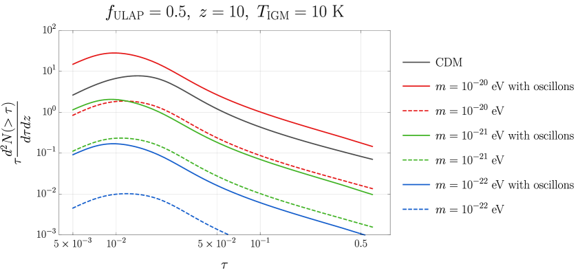
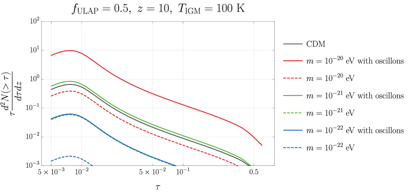
Figure 5: The adundance of 21cm absorbers. The upper and lower figures show the case of $T_{\rm IGM}=10\ {\rm K},100\ {\rm K}$ respectively. The horizontal axis shows the optical depth and the vertical axis does abundance of the number of systems intersected with the optical depth $\tau$ per redshift interval. The red, green, and blue lines show the result of $m=10^{-20}\ {\rm eV},\ m=10^{-21}\ {\rm eV},$ and $m=10^{-22}\ {\rm eV}$. and the solid and dashed lines show the halo mass function with ULAP oscillons and without ULAP oscillon respectively. We also plotted the result of $\Lambda$CDM model as the black line for comparison.

From the above relations, we can derive the number of systems intersected with the optical depth greater than $\tau$ per redshift interval as

$$\frac{dN(>\tau)}{dz}=(1+z)^{2}\frac{dr}{dz}\int_{M_{\rm min}}^{M_{\rm max}}n(M,z)\pi\alpha(\tau)^{2}dM,$$ (3.27)

where $dr/dz=c/H(z)$ is the comoving line element and $\alpha(\tau)$ shows the maximum physical radius where the optical depth exceeds $\tau$. As the halo mass function, we will use the matter power spectrum derived in Sec. 2.

The upper and lower bounds of the integration have a great effect on the abundance. The minimum mass of the minihalo $M_{\rm min}$ should be determined by the Jeans scale of IGM, which leads to

$$M_{\rm min}=\frac{4\pi\rho_{m}(z)}{3}\left(\frac{5\pi k_{B}T_{\rm IGM}}{3G\mu\rho_{m}(z)}\right)^{3/2}\simeq 3.58\times 10^{5}h^{-1}M_{\odot}\left(\frac{T_{\rm IGM}/K}{1+z}\right)^{3/2}.$$ (3.28)

where $T_{\rm IGM}$ is the IGM temperature. The IGM temperature around $z\sim 10$ is still unclear because of the uncertainties of the astrophysics. In this paper, we choose $T_{\rm IGM}=10\ {\rm K},100\ {\rm K}$ which avoid recent constraints on $T_{\rm IGM}$ [52, 53].

The maximum mass $M_{\rm max}$ is determined by the condition

$$T_{\rm vir}\left(M\right)\apprle 10^{4}\ {\rm K}.$$ (3.29)

Below this temperature, the star formation becomes inefficient because of the weakness of the metal-free gas cooling [48, 55]. The corresponding mini-halo mass is about $3\times 10^{7}M_{\odot}$.

The result of the calculation is shown in Fig. 5. All dashed lines (ALP without oscillons) are smaller than the CDM case because the number of mini-halos is suppressed by homogeneous ULAP as mentioned in Sec. 2. On the other hand, the solid lines (ALP with oscillons) are larger than the dashed lines due to the enhanced number of mini-halos with $10^{6}M_{\odot}\lesssim M\lesssim 10^{7}M_{\odot}$. Because the number of intersections is smaller than $1$ when $m\lesssim 10^{-21}\text{eV}$ even for ULAP oscillons with $T_{\rm IGM}=10\ {\rm K}$, it could be difficult to observe the difference of the 21cm absorption lines in this range. The range becomes smaller when the IGM temperature is larger as shown in the lower figure of Fig. 5, but this result still contains various uncertainties in $T_{\rm IGM}$ and the mini-halo profile. Thus, we should wait for observational and theoretical progress for more precise estimation.

4 Discussion

Detectability

We plotted the parameter region of ULAP that can be detectable by 21cm forest in Fig. 6. We have considered the following constraints in the figure.

• ULAP abundance: Because the energy density at the oscillon formation is determined by the lattice simulation, we can constrain the ULAP parameters by requiring $f_{\rm ULAP}<1$, which excludes the blue region in Fig. 6. Note that this constraint would be changed depending on the initial value of the ULAP. It would be stricter when the initial amplitude becomes larger than our simulation value $\phi_{i}/F=12\pi$, and vice versa.

• Oscillon lifetime: The produced oscillons must live up to the observation time ($z=10$ in this paper) because the density fluctuation may be smeared out after the oscillon decay due to the self-radiation. This constraint for $p=-3/4$ is shown as the red region in Fig. 6.

• Observations of matter power spectrum: The matter power spectrum on the large scale $k\lesssim\mathcal{O}(1)\ {\rm Mpc^{-1}}$ is precisely determined by many observations, such as Planck [6], DES [5], and SDSS [56, 57]. Thus, we constrain the ULAP parameters by the condition $P_{\rm osc}(1/{\rm Mpc})>P_{\rm\Lambda CDM}(1/{\rm Mpc})$ as the green region in Fig. 6. We did not include the Lyman-$\alpha$ constraint discussed in Refs. [58, 59] here because it is not obvious whether the produced oscillons affect the result of their simulations.

• The amplitude of the oscillon matter power spectrum: To detect the difference between the ULAP oscillon and the ordinary $\Lambda$CDM, the amplitude of the oscillon matter power spectrum must be at least larger than that of $\Lambda$CDM model. Thus, the region $P_{\rm osc}(k_{\rm cut})<P_{\Lambda{\rm CDM}}(k_{\rm cut})$ is conservatively excluded where $k_{\rm cut}$ is the cut-off wavenumber mentioned in Sec. 2. This constraint is shown as the orange region in Fig. 6 and we find that ULAP is detectable if $f_{\rm ULAP}\gg 10^{-2}$.

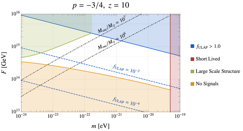
Figure 6: The detectable parameter region by 21cm forest with ULAP oscillons. The horizontal and vertical axis show the ULAP mass and the ULAP decay constant, respectively. The blue region is excluded because the ULAP abundance $f_{\rm ULAP}$ is larger than $1$ when the initial amplitude of ULAP is $\phi_{i}/F=12\pi$. The red region shows the case that the lifetime of produced oscillons for $p=-3/4$ is smaller than the cosmic time at $z=10$. The green region is excluded by the condition $P_{\rm osc}(1/{\rm Mpc})>P_{\Lambda{\rm CDM}}(1/{\rm Mpc})$ because the matter power spectrum on the large scale $\lesssim\mathcal{O}(1)\ {\rm Mpc}^{-1}$ is constrained by observations. The orange region is excluded by $P_{\rm osc}(k_{\rm cut})<P_{\Lambda{\rm CDM}}(k_{\rm cut})$ where $k_{\rm cut}$ is the cut-off wavenumber determined by the number of oscillon as mentioned in Sec. 2.

Mini-halo profile

When $p=-3/4$, the average oscillon mass at $z=10$ is

$$M_{\rm osc}\sim 6\times 10^{6}M_{\odot}\left(\frac{F}{10^{15}\ {\rm GeV}}\right)^{2}\left(\frac{10^{-22}\ {\rm eV}}{m}\right).$$ (4.1)

while the interested mini-halo mass range is $10^{6}M_{\odot}\lesssim M\lesssim 10^{7}M_{\odot}$. The contours of the constant oscillon mass $10^{6}M_{\odot}$ and $10^{7}M_{\odot}$ are plotted in Fig. 6 as black dotted lines. Between these lines, the NFW profile may not describe the internal structure of the mini-halo well because the mini-halo mass is almost the same as the produced oscillon mass. In this case, the mini-halo profile becomes more centered by oscillons, which results in more absorption abundance near the mini-halo center. However, it is unclear whether oscillons are disrupted by the gravitational force in the matter dominated era. Thus, we used the NFW profile here and we will work on the gravitational stability of oscillons in future work.

Finally, we briefly comment on the existence of radio-loud sources in $z\gtrsim 10$ required for 21cm forest observations. Recently, the radio loud sources around $z\sim 6$ with a flux $\gtrsim\mathcal{O}(10)\ {\rm mJy}$ sufficient for Square Kilometer Array (SKA) observations [60] have been confirmed [61, 62] and a simple estimation indicates $10^{4}\sim 10^{5}$ quasars around $z\simeq 10$ in the whole sky per redshift interval [63, 31, 32]. Besides, Population (Pop) III stars have been proposed to produce GRBs [64, 65, 66, 67], which could be unique sources in the high-redshift universe. These possibilities support the importance of studies on the 21cm forest.

5 Conclusion

In this paper, we calculated the abundance of 21cm absorption lines when ULAP partially exists in the form of oscillons. Because the structure on a scale determined by ULAP mass is significantly affected by oscillons, the abundance of 21cm absorption lines is also changed. We found that the matter power spectrum can be affected when the ULAP mass is $m\lesssim 10^{-19}\ {\rm eV}$ and the ULAP fraction is $f_{\rm ULAP}\gg 10^{-2}$. This result is applicable to all ULAP models which produce long-lived oscillons.

Unlike the previous researches, because the Poisson-like power spectrum is cut off by the energy conservation on large scale, we can focus on the phenomenologically interesting region $m\sim 10^{-22}\ {\rm eV}$ in this case. Besides, because the oscillons produce large fluctuations on a certain scale, ULAP can be detectable even if $f_{\rm ULAP}$ is smaller than $1$.

In this paper, we only focus on oscillons that survive at the observation time $z=10$. However, the relativistic ULAP emitted by the complete decay of oscillons smears out the structure of the horizon scale like warm dark matter, which may give us another constraint on ULAP to consider. This problem remains as future work.

Appendix A Oscillon Matter Power Spectrum

In this appendix, we briefly introduce the analytical formula of the oscillon matter power spectrum at oscillon formation Eq. (2.5). For simplicity, we will ignore the size of oscillons and treat them as a point-like mass. Thus, the derivation below is independent of the oscillon profile.

Let us consider a box with a comoving volume $V$ in which the number of oscillons with mass $M_{i}$ is represented by $N_{i}$. When the positions of oscillons are not correlated, $N_{i}$ follows the Poisson distribution, i.e.

$$\Braket{(N_{i}-\braket{N_{i}})(N_{j}-\braket{N_{j}})}_{N}=\braket{N_{i}}_{N}\delta_{ij},$$ (A.1)

where $\langle\rangle_{N}$ is statistical average over $N_{i}$. Given that the density contrast is represented by

$$\delta=\frac{\sum_{i}N_{i}M_{i}-\braket{\sum_{i}N_{i}M_{i}}_{N}}{\braket{\sum_{i}N_{i}M_{i}}_{N}},$$ (A.2)

and the physical number density of oscillons is

$$n_{\rm osc}=\frac{\sum_{i}\braket{N_{i}}_{N}}{a^{3}V},$$ (A.3)

the oscillon power spectrum at $k=2\pi V^{-1/3}$ is derived as

$$P_{\rm osc}(\bm{k}) =V\braket{\delta^{2}}_{N}$$ (A.4)

$$=V\frac{1}{\braket{\sum_{i}N_{i}M_{i}}_{N}^{2}}\sum_{i,j}M_{i}M_{j}\Braket{(N_{i}-\braket{N_{i}})(N_{j}-\braket{N_{j}})}_{N}$$ (A.5)

$$=V\frac{1}{\braket{\sum_{i}N_{i}M_{i}}_{N}^{2}}\sum_{i}M_{i}^{2}\braket{N_{i}}_{N}$$ (A.6)

$$=\frac{1}{n_{\rm osc}a^{3}}\frac{\Braket{M^{2}}}{\braket{M}^{2}}$$ (A.7)

where we have defined the average of the oscillon mass and squared oscillon mass as

$$\braket{M}\equiv\frac{\sum_{i}M_{i}\braket{N_{i}}_{N}}{\sum_{i}\braket{N_{i}}_{N}},\quad\Braket{M^{2}}\equiv\frac{\sum_{i}M_{i}^{2}\braket{N_{i}}_{N}}{\sum_{i}\braket{N_{i}}_{N}}.$$ (A.8)

Note that the statistical average over $N_{i}$ is substituted by the simulation result in this paper.

In the above calculation, we have assumed that each oscillon number $N_{i}$ follows the Poisson distribution, but the energy conservation constrains it when the box size $V$ is larger than the scale of the energy transfer at oscillon formation. Suppose the scale as $L_{s}$, the power spectrum is obtained with the suppression factor [33] as

$$P_{\rm osc}(\bm{k}) =\frac{1}{n_{\rm osc}a^{3}}\frac{\Braket{M^{2}}}{\braket{M}^{2}}K(kL_{s}),$$ (A.9)

$$K(x) =\left[1-\left(\frac{2}{x}\right)^{2}\sin^{2}\left(\frac{x}{2}\right)\right],$$ (A.10)

which corresponds to Eq. (2.5) except for the overall factor related to the energy fraction.

Appendix B Simulation Setup

Table 1: Simulation parameters.

$p$	$-3/4$
Box size $L$	$32$
Grid size $N$	$1024^{3}$
Time	$1-81$
Time step	$8\times 10^{-3}$

In the simulation, the units of the field, the conformal time, and the space, etc. are taken to be $F$ and $m^{-1}$, that is,

$$\bar{\phi}\equiv\frac{\phi}{F},\ \ \bar{\tau}\equiv m\tau,\ \ \bar{x}\equiv mx,\ \ \dots\ {\rm etc}.$$ (B.1)

where the overline denotes the dimensionless program variables and $\tau$ is the conformal time.

As the initial condition, we take the initial Hubble parameter as $H_{i}=1/2t=m$ because ULAP starts to oscillate in the radiation dominated universe. The initial scale factor is set to be unity $a_{i}=1$, related to the conformal time as $a=\bar{\tau}$. The initial field value and its derivative are set as

$$\bar{\phi}_{i}(\bm{x})=12\pi(1+\zeta(\bm{x})),\quad\bar{\phi}_{i}(\bm{x})^{\prime}=0,$$ (B.2)

where dash represents the derivative with $\bar{\tau}$ and $\zeta(\bm{x})$ is the initial noise defined by the scale-free power spectrum

$$\langle\xi_{\bm{k}}\xi_{\bm{k}^{\prime}}\rangle=(2\pi)^{3}\delta^{3}(\bm{k}-\bm{k}^{\prime})\frac{2\pi^{2}}{k^{3}}\mathcal{P}_{\xi},$$ (B.3)

with a small constant $\mathcal{P}_{\xi}=2.1\times 10^{-9}$ as a reference value. Other simulation parameters are shown in Table 1.

We utilize our lattice simulation code used in Refs. [20, 24, 26], in which the time evolution is calculated by the fourth-order symplectic integration scheme and the spatial derivatives are calculated by the fourth-order central difference scheme. We impose the periodic boundary condition on the boundary.

References

- [1] K. Begeman, A. Broeils and R. Sanders, Extended rotation curves of spiral galaxies: Dark haloes and modified dynamics, Mon. Not. Roy. Astron. Soc. 249 (1991) 523.
- [2] M. Mateo, Dwarf galaxies of the Local Group, Ann. Rev. Astron. Astrophys. 36 (1998) 435–506, [astro-ph/9810070].
- [3] L. Koopmans and T. Treu, The structure and dynamics of luminous and dark matter in the early-type lens galaxy of 0047-281 at z=0.485, Astrophys. J. 583 (2003) 606–615, [astro-ph/0205281].
- [4] WMAP collaboration, G. Hinshaw et al., Nine-Year Wilkinson Microwave Anisotropy Probe (WMAP) Observations: Cosmological Parameter Results, Astrophys. J. Suppl. 208 (2013) 19, [1212.5226].
- [5] DES collaboration, T. Abbott et al., Dark Energy Survey year 1 results: Cosmological constraints from galaxy clustering and weak lensing, Phys. Rev. D 98 (2018) 043526, [1708.01530].
- [6] Planck collaboration, N. Aghanim et al., Planck 2018 results. VI. Cosmological parameters, 1807.06209.
- [7] B. Moore, S. Ghigna, F. Governato, G. Lake, T. R. Quinn, J. Stadel et al., Dark matter substructure within galactic halos, Astrophys. J. Lett. 524 (1999) L19–L22, [astro-ph/9907411].
- [8] W. de Blok, The Core-Cusp Problem, Adv. Astron. 2010 (2010) 789293, [0910.3538].
- [9] M. Boylan-Kolchin, J. S. Bullock and M. Kaplinghat, The Milky Way’s bright satellites as an apparent failure of LCDM, Mon. Not. Roy. Astron. Soc. 422 (2012) 1203–1218, [1111.2048].
- [10] J. S. Bullock and M. Boylan-Kolchin, Small-Scale Challenges to the CDM Paradigm, Ann. Rev. Astron. Astrophys. 55 (2017) 343–387, [1707.04256].
- [11] P. Svrcek and E. Witten, Axions In String Theory, JHEP 06 (2006) 051, [hep-th/0605206].
- [12] W. Hu, R. Barkana and A. Gruzinov, Cold and fuzzy dark matter, Phys. Rev. Lett. 85 (2000) 1158–1161, [astro-ph/0003365].
- [13] L. Hui, J. P. Ostriker, S. Tremaine and E. Witten, Ultralight scalars as cosmological dark matter, Phys. Rev. D 95 (2017) 043541, [1610.08297].
- [14] I. L. Bogolyubsky and V. G. Makhankov, Lifetime of Pulsating Solitons in Some Classical Models, Pisma Zh. Eksp. Teor. Fiz. 24 (1976) 15–18.
- [15] M. Gleiser, Pseudostable bubbles, Phys. Rev. D49 (1994) 2978–2981, [hep-ph/9308279].
- [16] E. J. Copeland, M. Gleiser and H. R. Muller, Oscillons: Resonant configurations during bubble collapse, Phys. Rev. D52 (1995) 1920–1933, [hep-ph/9503217].
- [17] M. A. Amin, R. Easther, H. Finkel, R. Flauger and M. P. Hertzberg, Oscillons After Inflation, Phys. Rev. Lett. 108 (2012) 241302, [1106.3335].
- [18] M. A. Amin, R. Easther and H. Finkel, Inflaton Fragmentation and Oscillon Formation in Three Dimensions, JCAP 12 (2010) 001, [1009.2505].
- [19] M. A. Amin and P. Mocz, Formation, gravitational clustering, and interactions of nonrelativistic solitons in an expanding universe, Phys. Rev. D 100 (2019) 063507, [1902.07261].
- [20] M. Ibe, M. Kawasaki, W. Nakano and E. Sonomoto, Decay of I-ball/Oscillon in Classical Field Theory, JHEP 04 (2019) 030, [1901.06130].
- [21] H.-Y. Zhang, M. A. Amin, E. J. Copeland, P. M. Saffin and K. D. Lozanov, Classical Decay Rates of Oscillons, JCAP 07 (2020) 055, [2004.01202].
- [22] S. Kasuya, M. Kawasaki and F. Takahashi, I-balls, Phys. Lett. B559 (2003) 99–106, [hep-ph/0209358].
- [23] M. Kawasaki, F. Takahashi and N. Takeda, Adiabatic Invariance of Oscillons/I-balls, Phys. Rev. D92 (2015) 105024, [1508.01028].
- [24] M. Ibe, M. Kawasaki, W. Nakano and E. Sonomoto, Fragileness of Exact I-ball/Oscillon, Phys. Rev. D 100 (2020) 125021, [1908.11103].
- [25] J. Ollé, O. Pujolàs and F. Rompineve, Oscillons and Dark Matter, JCAP 02 (2020) 006, [1906.06352].
- [26] M. Kawasaki, W. Nakano and E. Sonomoto, Oscillon of Ultra-Light Axion-like Particle, JCAP 01 (2020) 047, [1909.10805].
- [27] P. Madau, A. Meiksin and M. J. Rees, 21-CM tomography of the intergalactic medium at high redshift, Astrophys. J. 475 (1997) 429, [astro-ph/9608010].
- [28] C. Carilli, N. Y. Gnedin and F. Owen, Hi 21cm absorption beyond the epoch of re-ionization, Astrophys. J. 577 (2002) 22–30, [astro-ph/0205169].
- [29] S. Furlanetto and A. Loeb, The 21 cm forest: Radio absorption spectra as a probe of the intergalactic medium before reionization, Astrophys. J. 579 (2002) 1–9, [astro-ph/0206308].
- [30] R. Barkana and A. Loeb, In the beginning: The First sources of light and the reionization of the Universe, Phys. Rept. 349 (2001) 125–238, [astro-ph/0010468].
- [31] H. Shimabukuro, K. Ichiki and K. Kadota, Constraining the nature of ultra light dark matter particles with the 21 cm forest, Phys. Rev. D 101 (2020) 043516, [1910.06011].
- [32] H. Shimabukuro, K. Ichiki and K. Kadota, 21 cm forest probes on axion dark matter in postinflationary Peccei-Quinn symmetry breaking scenarios, Phys. Rev. D 102 (2020) 023522, [2005.05589].
- [33] M. Kawasaki, W. Nakano, H. Nakatsuka and E. Sonomoto, Oscillons of Axion-Like Particle: Mass distribution and power spectrum, 2010.09311.
- [34] R. Hlozek, D. Grin, D. J. E. Marsh and P. G. Ferreira, A search for ultralight axions using precision cosmological data, Phys. Rev. D 91 (2015) 103512, [1410.2896].
- [35] A. Lewis, A. Challinor and A. Lasenby, Efficient computation of CMB anisotropies in closed FRW models, Astrophys. J. 538 (2000) 473–476, [astro-ph/9911177].
- [36] C. Howlett, A. Lewis, A. Hall and A. Challinor, Cmb power spectrum parameter degeneracies in the era of precision cosmology, Journal of Cosmology and Astroparticle Physics 2012 (2012) 027.
- [37] E. Silverstein and A. Westphal, Monodromy in the CMB: Gravity Waves and String Inflation, Phys. Rev. D78 (2008) 106003, [0803.3085].
- [38] L. McAllister, E. Silverstein and A. Westphal, Gravity Waves and Linear Inflation from Axion Monodromy, Phys. Rev. D82 (2010) 046003, [0808.0706].
- [39] Y. Nomura, T. Watari and M. Yamazaki, Pure Natural Inflation, Phys. Lett. B776 (2018) 227–230, [1706.08522].
- [40] H. Shimabukuro, K. Ichiki, S. Inoue and S. Yokoyama, Probing small-scale cosmological fluctuations with the 21 cm forest: Effects of neutrino mass, running spectral index, and warm dark matter, Phys. Rev. D 90 (2014) 083003, [1403.1605].
- [41] J. F. Navarro, C. S. Frenk and S. D. White, A Universal density profile from hierarchical clustering, Astrophys. J. 490 (1997) 493–508, [astro-ph/9611107].
- [42] J. F. Hennawi, N. Dalal, P. Bode and J. P. Ostriker, Characterizing the cluster lens population, Astrophys. J. 654 (2007) 714–730, [astro-ph/0506171].
- [43] J. M. Comerford and P. Natarajan, The Observed Concentration-Mass Relation for Galaxy Clusters, Mon. Not. Roy. Astron. Soc. 379 (2007) 190–200, [astro-ph/0703126].
- [44] J. S. Bullock, T. S. Kolatt, Y. Sigad, R. S. Somerville, A. V. Kravtsov, A. A. Klypin et al., Profiles of dark haloes. Evolution, scatter, and environment, Mon. Not. Roy. Astron. Soc. 321 (2001) 559–575, [astro-ph/9908159].
- [45] A. Cooray and R. K. Sheth, Halo Models of Large Scale Structure, Phys. Rept. 372 (2002) 1–129, [astro-ph/0206508].
- [46] N. Makino, S. Sasaki and Y. Suto, X-ray gas density profile of clusters of galaxies from the universal dark matter halo, Astrophys. J. 497 (1998) 555, [astro-ph/9710344].
- [47] W. H. Press and P. Schechter, Formation of galaxies and clusters of galaxies by selfsimilar gravitational condensation, Astrophys. J. 187 (1974) 425–438.
- [48] R. K. Sheth and G. Tormen, Large scale bias and the peak background split, Mon. Not. Roy. Astron. Soc. 308 (1999) 119, [astro-ph/9901122].
- [49] G. B. Field, Excitation of the hydrogen 21-cm line, Proceedings of the IRE 46 (1958) 240–250.
- [50] B. Zygelman, Hyperfine level–changing collisions of hydrogen atoms and tomography of the dark age universe, The Astrophysical Journal 622 (apr, 2005) 1356–1362.
- [51] S. Furlanetto, S. Oh and F. Briggs, Cosmology at Low Frequencies: The 21 cm Transition and the High-Redshift Universe, Phys. Rept. 433 (2006) 181–301, [astro-ph/0608032].
- [52] B. Greig et al., Interpreting LOFAR 21-cm signal upper limits at z~9.1 in the context of high-z galaxy and reionisation observations, 2006.03203.
- [53] B. Greig, C. M. Trott, N. Barry, S. J. Mutch, B. Pindor, R. L. Webster et al., Exploring reionisation and high-z galaxy observables with recent multi-redshift MWA upper limits on the 21-cm signal, 2008.02639.
- [54] P. Madau and M. Kuhlen, The dawn of galaxies, in Multiwavelength Mapping of Galaxy Evolution, ESO Astrophysics Symposia European Southern Observatory, pp. 1–11, 2005, astro-ph/0303584, DOI.
- [55] I. T. Iliev, P. R. Shapiro, A. Ferrara and H. Martel, On the direct detectability of the cosmic dark ages: 21-cm emission from minihalos, Astrophys. J. 572 (2002) 123, [astro-ph/0202410].
- [56] B. M. R. et al., Sloan Digital Sky Survey IV: Mapping the Milky Way, Nearby Galaxies, and the Distant Universe, The Astronomical Journal 154 (July, 2017) 28, [1703.00052].
- [57] B. Abolfathi et al., The fourteenth data release of the sloan digital sky survey: First spectroscopic data from the extended baryon oscillation spectroscopic survey and from the second phase of the apache point observatory galactic evolution experiment, The Astrophysical Journal Supplement Series 235 (Apr., 2018) 42, [1707.09322].
- [58] V. Iršič, M. Viel, M. G. Haehnelt, J. S. Bolton and G. D. Becker, First constraints on fuzzy dark matter from Lyman- forest data and hydrodynamical simulations, Phys. Rev. Lett. 119 (2017) 031302, [1703.04683].
- [59] T. Kobayashi, R. Murgia, A. De Simone, V. Iršič and M. Viel, Lyman- constraints on ultralight scalar dark matter: Implications for the early and late universe, Phys. Rev. D 96 (2017) 123514, [1708.00015].
- [60] S. Furlanetto, The 21 Centimeter Forest, Mon. Not. Roy. Astron. Soc. 370 (2006) 1867–1875, [astro-ph/0604223].
- [61] E. Bañados, C. Carilli, F. Walter, E. Momjian, R. Decarli, E. P. Farina et al., A powerful radio-loud quasar at the end of cosmic reionization, The Astrophysical Journal 861 (Jul, 2018) L14.
- [62] S. Belladitta et al., The first blazar observed at z 6, Astron. Astrophys. 635 (2020) L7, [2002.05178].
- [63] Y. Xu, X. Chen, Z. Fan, H. Trac and R. Cen, THE 21 cm FOREST AS a PROBE OF THE REIONIZATION AND THE TEMPERATURE OF THE INTERGALACTIC MEDIUM, The Astrophysical Journal 704 (oct, 2009) 1396–1404.
- [64] S. S. Komissarov and M. V. Barkov, Supercollapsars and their X-ray bursts, Monthly Notices of the Royal Astronomical Society: Letters 402 (02, 2010) L25–L29, [https://academic.oup.com/mnrasl/article-pdf/402/1/L25/4894965/402-1-L25.pdf].
- [65] K. Toma, T. Sakamoto and a. Mészáros, Population iii gamma-ray burst afterglows: Constraints on stellar masses and external medium densities, The Astrophysical Journal 731 (04, 2011) 127.
- [66] P. Meszaros and M. Rees, Population III Gamma Ray Bursts, Astrophys. J. 715 (2010) 967–971, [1004.2056].
- [67] Y. Suwa and K. Ioka, Can Gamma-Ray Burst Jets Break Out the First Stars?, Astrophys. J. 726 (2011) 107, [1009.6001].