A measure concentration effect for matrices of high, higher, and even higher dimension

Abstract

Let $n>m$, and let $A$ be an $(m\times n)$-matrix of full rank. Then obviously the estimate $\|Ax\|\leq\|A\|\|x\|$ holds for the euclidean norm of $x$ and $Ax$ and the spectral norm as the assigned matrix norm. We study the sets of all $x$ for which, for fixed $\delta<1$, conversely $\|Ax\|\geq\delta\,\|A\|\|x\|$ holds. It turns out that these sets fill, in the high-dimensional case, almost the complete space once $\delta$ falls below a bound that depends on the extremal singular values of $A$ and on the ratio of the dimensions. This effect has much to do with the random projection theorem, which plays an important role in the data sciences. As a byproduct, we calculate the probabilities this theorem deals with exactly.

15A99, 15B52, 60B20

1 Introduction

Let $n>m$ and let $A$ be a real $(m\times n)$-matrix of rank $m$. The kernel of such a matrix has the dimension $n-m$ and hence can, in dependence of the dimensions, be a large subspace of the $\mathbb{R}^{n}$. Nevertheless, the set of all $x$ for which

(1) $$\|Ax\|\geq\delta\,\|A\|\|x\|$$

holds fills, in the high-dimensional case, often almost the complete $\mathbb{R}^{n}$ once $\delta$ falls below a certain bound; the involved norms are here and throughout the paper the euclidean norm on the $\mathbb{R}^{m}$ and the $\mathbb{R}^{n}$ and the assigned spectral norm of matrices. Let $\chi$ be the characteristic function of the set of all $x$ for which $\|Ax\|<\delta\,\|A\|\|x\|$ holds, and let $\nu_{n}$ be the volume of the unit ball in $\mathbb{R}^{n}$. The normed area measure

(2) $$\frac{1}{n\nu_{n}}\int_{S^{n-1}}\!\chi(\eta)\,\mathrm{d}\eta$$

of the subset of the unit sphere on which the condition (1) is violated takes in such cases an extremely small value, which conversely again means that (1) holds on an overwhelmingly large part of the unit sphere and with that of the full space. The aim of the present paper is to study this phenomenon in dependence of characteristic quantities like the ratio of the dimensions $m$ and $n$ and the extremal singular values of the matrices qualitatively and, as far as possible, also quantitatively.

The described effect is best understood for orthogonal projections. For matrices of this kind, this observation is a direct consequence of the random projection theorem (see Lemma 5.3.2 in [13], for example), which is in close connection with the Johnson–Lindenstrauss theorem [6]. The random projection theorem deals with orthogonal projections from the $\mathbb{R}^{n}$ onto random subspaces of lower dimension $m$, but equally one can consider orthogonal projections $Px$ of random vectors $x$ to the $\mathbb{R}^{m}$. The theorem states that with probability greater than $1-2\exp(-c\,\varepsilon^{2}m)$

(3) $$(1-\varepsilon)\sqrt{\frac{m}{n}}\,\|x\|\leq\|Px\|\leq(1+\varepsilon)\sqrt{\frac{m}{n}}\,\|x\|$$

holds for all $x$ on the unit sphere and thereby also in the full space. The random projection theorem is a manifestation of the concentration of measure phenomenon, which plays a fundamental role in the analysis of very many problems in high space dimensions and became a backbone of high-dimensional probability theory and modern data science. The interest in the concentration of measure phenomenon arose in the early 1970s in the study of the asymptotic theory of Banach spaces. Classical texts are [7] and [8]. An up-to-date exposition containing a lot of information on random vectors and matrices is [13]. In the present article, we carefully reconsider the random projection theorem. Among other things, we calculate the normed area measure (2) for projection matrices of the described kind for even-numbered differences of the two dimensions exactly and derive a very sharp inclusion for the odd-numbered case. The results for these projection matrices serve as a basis for the examination of general matrices in dependence of their singular values.

One might ask what is known about these. The simple answer is that this depends on the class of matrices one considers. Graph theory [1], [2] is an important source of information. There is an extensive literature about the extremal singular values of random matrices with independent, identically distributed entries. An early breakthrough was Edelman’s thesis [3]. Other significant contributions are [11], [12], and, very recently, [9]. Random matrices play an important role in fields like compressed sensing [4] and all sorts of data acquisition and compression techniques. Our interest in the problem originates from the attempt [14] to extend the applicability of modern tensor product methods [5] to more general problem classes. Assume that we are looking for the solution $u:\mathbb{R}^{m}\to\mathbb{R}$ of the Laplace-like equation

(4) $$-\Delta u+\mu u=f$$

that vanishes at infinity, where $\mu>0$ is constant and the right-hand side $f$ is, for instance, a product of functions depending only on a single component of $x$ or on the difference of two such components. The question is how well such structures are reflected in the solution of the equation.

Let us assume that the right-hand side is of the form $f(x)=F(Tx)$, with a function $F:\mathbb{R}^{n}\to\mathbb{R}$, $n>m$, with an integrable Fourier transform and with $T$ a matrix of full rank that is determined by the structure of the underlying problem. As shown in [14], the solution is then the trace $u(x)=U(Tx)$ of the function

(5) $$U(y)=\Big{(}\frac{1}{\sqrt{2\pi}}\Big{)}^{n}\!\int\frac{1}{\mu+\|T^{t}\omega\|^{2}}\,\widehat{F}(\omega)\,\mathrm{e}^{\,\mathrm{i}\,\omega\cdot y}\,\mathrm{d}\omega.$$

The function (5) is in the domain of the operator $\mathcal{L}$ given by

(6) $$(\mathcal{L}U)(y)=\Big{(}\frac{1}{\sqrt{2\pi}}\Big{)}^{n}\!\int\big{(}\mu+\|T^{t}\omega\|^{2}\big{)}\widehat{U}(\omega)\,\mathrm{e}^{\,\mathrm{i}\,\omega\cdot y}\,\mathrm{d}\omega$$

and solves by definition the degenerate second-order elliptic equation $\mathcal{L}U=F$. It can be calculated approximately by means of the iteration

(7) $$U_{k+1}=(I-\alpha\mathcal{L})U_{k}+\alpha F,$$

where the operator $\alpha$ is given by

(8) $$(\alpha F)(y)=\Big{(}\frac{1}{\sqrt{2\pi}}\Big{)}^{n}\!\int\frac{1}{\mu+\|T^{t}\|^{2}\|\omega\|^{2}}\,\widehat{F}(\omega)\,\mathrm{e}^{\,\mathrm{i}\,\omega\cdot y}\,\mathrm{d}\omega.$$

Provided that $\|T^{t}\omega\|\geq\delta\,\|T^{t}\|\|\omega\|$ holds on the support of $\widehat{F}$, the $L_{1}$-norm of the Fourier transform of the error is in every iteration step reduced by the factor $1-\delta^{2}$, or by more than the factor $1-\delta$ with polynomial acceleration. If this condition is only violated on a very small set, the additional error can in general be neglected without hard conditions to $\widehat{F}$ or $F$ itself. The idea is to approximate the kernel in (8) by a linear combination of Gauss functions. If $F$ is as in the example above the product of lower-dimensional functions depending only on small groups of components of $Tx$, the iterates are then composed of functions of the same type.

2 Reformulations as volume integrals and first estimates

The surface integrals (2) are not easily accessible and are difficult to calculate and estimate. We reformulate them therefore at first as volume integrals and draw some first conclusions from these representations. The starting point is the decomposition

(1) $$\int_{\mathbb{R}^{n}}f(x)\,\mathrm{d}x\,=\int_{S^{n-1}}\left(\int_{0}^{\infty}\!f(r\eta)r^{n-1}\,\mathrm{d}r\right)\!\,\mathrm{d}\eta$$

of the integrals of functions in $L_{1}$ into an inner radial and an outer angular part. Inserting the characteristic function of the unit ball, one recognizes that the area of the $n$-dimensional unit sphere is $n\nu_{n}$, with $\nu_{n}$ the volume of the unit ball. If $f$ is rotationally symmetric, $f(r\eta)=f(re)$ holds for every $\eta\in S^{n-1}$ and every fixed, arbitrarily given unit vector $e$. In this case, (1) reduces therefore to

(2) $$\int f(x)\,\mathrm{d}x\,=n\nu_{n}\int_{0}^{\infty}\!f(re)r^{n-1}\,\mathrm{d}r.$$

The volume measure on the $\mathbb{R}^{n}$ will in the following be denoted by $\lambda$.

Lemma 2.1.

Let $A$ be an arbitrary matrix of dimension $m\times n$, $m<n$, let $\chi$ be the characteristic function of the set of all $x\in\mathbb{R}^{n}$ for which $\|Ax\|<\delta\,\|A\|\|x\|$ holds, and let $W:\mathbb{R}^{n}\to\mathbb{R}$ be a rotationally symmetric function with integral

(3) $$\int W(x)\,\mathrm{d}x\,=\,1.$$

The weighted surface integral (2) then takes the value

(4) $$\int\chi(x)W(x)\,\mathrm{d}x.$$

Proof 2.2.

Let $e$ be a given unit vector. For $\eta\in S^{n-1}$ and $r>0$ then $\chi(r\eta)=\chi(\eta)$ and $W(r\eta)=W(re)$ holds and the integral (4) can by (1) be written as

$$\int\chi(x)W(x)\,\mathrm{d}x\,=\int_{S^{n-1}}\chi(\eta)\left(\int_{0}^{\infty}\!W(re)r^{n-1}\,\mathrm{d}r\right)\!\,\mathrm{d}\eta.$$

Because the inner integral takes by (2) and (3) the value

$$\int_{0}^{\infty}\!W(re)r^{n-1}\,\mathrm{d}r=\frac{1}{n\nu_{n}},$$

this proves the proposition.

An obvious choice for the weight function $W$, which will later still play an important role and will be used at several places, is the normed Gauss function

(5) $$W(x)=\Big{(}\frac{1}{\sqrt{\pi}}\Big{)}^{n}\exp\big{(}-\|x\|^{2}\big{)}.$$

Another possible choice is the characteristic function of the ball of radius $R$ around the origin divided by the volume of this ball. It leads to the following lemma.

Lemma 2.3.

Let $A$ be a matrix of dimension $m\times n$, $m<n$, and let $\lambda$ be the volume measure on the $\mathbb{R}^{n}$. The weighted integral (2) over the surface of the unit ball is then independent of the radius $R$ equal to the volume ratio

(6) $$\frac{\lambda\big{(}\big{\{}x\,\big{|}\,\|Ax\|<\delta\,\|A\|\|x\|,\,\|x\|\leq R\big{\}}\big{)}}{\lambda\big{(}\big{\{}x\,\big{|}\,\|x\|\leq R\big{\}}\big{)}}.$$

Because the euclidean length of a vector and the volume of a set are invariant to orthogonal transformations, the surface ratio (2) and the volume ratio (6) as well depend only on the singular values of the matrix under consideration.

Lemma 2.4.

Let $A$ be a matrix of dimension $m\times n$, $m<n$, with singular value decomposition $A=U\Sigma V^{t}$. The volume ratios (6) are then equal to the volume ratios

(7) $$\frac{\lambda\big{(}\big{\{}x\,\big{|}\,\|\Sigma x\|<\delta\,\|\Sigma\|\|x\|,\,\|x\|\leq R\big{\}}\big{)}}{\lambda\big{(}\big{\{}x\,\big{|}\,\|x\|\leq R\big{\}}\big{)}};$$

that is, they depend exclusively on the singular values of the matrix $A$.

Proof 2.5.

As the multiplication with the orthogonal matrices $U$ and $V^{t}$, respectively, does not change the euclidean norm of a vector, the set of all $x\in\mathbb{R}^{n}$ for which

$$\|Ax\|<\delta\,\|A\|\|x\|,\quad\|x\|\leq R,$$

holds coincides with the set of all $x$ for which we have

$$\|\Sigma V^{t}x\|<\delta\,\|\Sigma\|\|V^{t}x\|,\quad\|V^{t}x\|\leq R.$$

As the volume is invariant to orthogonal transformations, the proposition follows.

Orthogonal projections, or in other words matrices with one as the only singular value, represent one of the few cases for which the volume ratios (6) can be more or less explicitly calculated. Orthogonal projections are of particular importance and will, as said, serve as the anchor for many of our estimates. Again, it suffices to consider the corresponding diagonal matrices $\Sigma$, denoted in the following by $P$.

Theorem 2.6.

Let $P$ be the $(m\times n)$-matrix that extracts from a vector in $\mathbb{R}^{n}$ its first $m$ components. For $0\leq\delta<1$ and all radii $R>0$, then

(8) $$\frac{\lambda\big{(}\big{\{}x\,\big{|}\,\|Px\|<\delta\,\|x\|,\,\|x\|\leq R\big{\}}\big{)}}{\lambda\big{(}\big{\{}x\,\big{|}\,\|x\|\leq R\big{\}}\big{)}}=\psi\bigg{(}\frac{\delta}{\sqrt{1-\delta^{2}}}\bigg{)}$$

holds, where the function $\psi$ is defined by the integral expression

(9) $$\psi(\varepsilon)=\frac{2\,\Gamma(n/2)}{\Gamma(m/2)\Gamma((n-m)/2)}\int_{0}^{\varepsilon}\frac{t^{m-1}}{(1+t^{2})^{n/2}}\,\mathrm{d}t.$$

Proof 2.7.

Differing from the notation in the theorem but consistent within the proof, we split the vectors in $\mathbb{R}^{n}$ into parts $x\in\mathbb{R}^{m}$ and $y\in\mathbb{R}^{n-m}$. The set whose volume has to be calculated consists then of the points in the given ball for which

$$\|x\|<\delta\,\Big{\|}\Big{(}\,\begin{matrix}x\\ y\end{matrix}\,\Big{)}\Big{\|}$$

or, resolved for the norm of the component $x\in\mathbb{R}^{m}$,

$$\|x\|<\varepsilon\,\|y\|,\quad\varepsilon=\frac{\delta}{\sqrt{1-\delta^{2}}},$$

holds. For homogeneity reasons, that is, by Lemma 2.3, we can restrict ourselves to the ball of radius $R=1$. The volume can then be expressed as double integral

$$\int\bigg{(}\int H\big{(}\varepsilon\|y\|-\|x\|\big{)}\chi\big{(}\|x\|^{2}+\|y\|^{2}\big{)}\,\mathrm{d}x\bigg{)}\,\mathrm{d}y,$$

where $H(t)=0$ for $t\leq 0$, $H(t)=1$ for $t>0$, $\chi(t)=1$ for $t\leq 1$, and $\chi(t)=0$ for arguments $t>1$. In terms of polar coordinates, that is, by (2), it reads as

$$(n-m)\nu_{n-m}\int_{0}^{\infty}\bigg{(}m\nu_{m}\int_{0}^{\varepsilon s}\chi\big{(}r^{2}+s^{2}\big{)}r^{m-1}\,\mathrm{d}r\bigg{)}s^{n-m-1}\,\mathrm{d}s,$$

with $\nu_{d}$ the volume of the $d$-dimensional unit ball. Substituting $t=r/s$ in the inner integral, the upper bound becomes independent of $s$ and the integral can be written as

$$(n-m)\nu_{n-m}\int_{0}^{\infty}\bigg{(}m\nu_{m}\,s^{m}\!\int_{0}^{\varepsilon}\chi\big{(}s^{2}(1+t^{2})\big{)}t^{m-1}\,\mathrm{d}t\bigg{)}s^{n-m-1}\,\mathrm{d}s,$$

and interchanging the order of integration, it attains finally the value

$$\frac{(n-m)\nu_{n-m}\,m\nu_{m}}{n}\int_{0}^{\varepsilon}\frac{t^{m-1}}{(1+t^{2})^{n/2}}\,\mathrm{d}t.$$

Dividing this by the volume $\nu_{n}$ of the unit ball itself and remembering that

$$\nu_{d}=\frac{2}{d}\,\frac{\pi^{d/2}}{\Gamma(d/2)},$$

this completes the proof of the theorem.

The following lemma describes the dependence of the volume ratio (8) on the dimensions $m$ and $n$. In conjunction with Theorem 3.3 below it can be used to enclose the volume ratio from both sides for uneven differences of the dimensions.

Lemma 2.8.

The volume ratio (8) decreases, for $n$ kept fixed, when $m$ increases, and it increases, for $m$ kept fixed, when $n$ increases.

Proof 2.9.

The set in the numerator on the left-hand side of (8) gets smaller when $m$ gets larger. This proves the first proposition. The argumentation for increasing dimension $n$ is more involved. It is based on the representation from Lemma 2.1 with the weight function (5). For $x\in\mathbb{R}^{n}$ and $y\in\mathbb{R}^{p}$, let

$$\chi(x,y)=\begin{cases}\,1,&\text{if $\|Px\|^{2}<\delta^{2}\big{(}\|x\|^{2}+\|y\|^{2}\big{)}$}\\ \,0,&\text{otherwise}.\end{cases}$$

By Lemma 2.1, the volume ratio (8) can then be written as the integral

$$\Big{(}\frac{1}{\sqrt{\pi}}\Big{)}^{n}\!\int\chi(x,0)\exp\big{(}-\|x\|^{2}\big{)}\,\mathrm{d}x$$

over the $\mathbb{R}^{n}$. This integral takes by Fubini’s theorem the same value as the integral

$$\Big{(}\frac{1}{\sqrt{\pi}}\Big{)}^{n+p}\!\int\chi(x,0)\exp\big{(}-\big{(}\|x\|^{2}+\|y\|^{2}\big{)}\big{)}\,\mathrm{d}(x,y)$$

over the $\mathbb{R}^{n}\times\mathbb{R}^{p}$ and can be estimated from above by the integral

$$\Big{(}\frac{1}{\sqrt{\pi}}\Big{)}^{n+p}\!\int\chi(x,y)\exp\big{(}-\big{(}\|x\|^{2}+\|y\|^{2}\big{)}\big{)}\,\mathrm{d}(x,y).$$

This integral takes by Lemma 2.1 the same value as the volume ratio (8) , with the original dimension $m$, but with the dimension $n$ now replaced by $n^{\prime}=n+p$.

The volume ratios (6) can be bounded from both sides in terms of the, as we will see, more or less explicitly known volumes ratios (8), i.e., of the function (9).

Theorem 2.10.

Let $n>m$, let $A$ be an $(m\times n)$-matrix of full rank, and let $\kappa$ be the condition number of $A$, the ratio of its maximum to its minimum singular value. If $\kappa\delta$ is less than one, then for all radii $R>0$ the upper estimate

(10) $$\frac{\lambda\big{(}\big{\{}x\,\big{|}\,\|Ax\|<\delta\,\|A\|\|x\|,\,\|x\|\leq R\big{\}}\big{)}}{\lambda\big{(}\big{\{}x\,\big{|}\,\|x\|\leq R\big{\}}\big{)}}\leq\psi\bigg{(}\frac{\kappa\delta}{\sqrt{1-\kappa^{2}\delta^{2}}}\bigg{)}$$

holds, where $\psi$ is the function (9). Without further conditions to $\delta<1$, conversely

(11) $$\frac{\lambda\big{(}\big{\{}x\,\big{|}\,\|Ax\|<\delta\,\|A\|\|x\|,\,\|x\|\leq R\big{\}}\big{)}}{\lambda\big{(}\big{\{}x\,\big{|}\,\|x\|\leq R\big{\}}\big{)}}\geq\psi\bigg{(}\frac{\delta}{\sqrt{1-\delta^{2}}}\bigg{)}.$$

holds. For orthogonal projections, that is, if $\kappa=1$, in both cases equality holds.

Proof 2.11.

We can restrict ourselves in the proof to the diagonal matrices $\Sigma$ from Lemma 2.4. The proposition follows then rather immediately from the inequalities

$$\sigma_{1}\|Px\|\leq\|\Sigma x\|\leq\sigma_{m}\|Px\|$$

and the fact that $\|\Sigma\|=\sigma_{m}$ comparing the corresponding volumes.

Undoubtedly, (10) and (11) are despite their generality in many cases rather poor estimates because they largely ignore the underlying geometry. If the singular values $\sigma_{1}\leq\sigma_{2}\leq\cdots\leq\sigma_{m}$ of the matrix $A$ cluster around $\sigma_{m}>0$ or are, up to very few, even equal to $\sigma_{m}$, the following lemma opens a way out and provides a remedy.

Lemma 2.12.

Let $\sigma_{k}=\sigma_{m}$ for all $k>m_{0}$ and let $P^{\prime}$ be the matrix that extracts from a vector $x\in\mathbb{R}^{n}$ its components $x_{k}$, $m_{0}<k\leq m$. The volume ratio (6) is then less than or at most equal to the volume ratio

(12) $$\frac{\lambda\big{(}\big{\{}x\,\big{|}\,\|P^{\prime}x\|<\delta\,\|x\|,\,\|x\|\leq R\big{\}}\big{)}}{\lambda\big{(}\big{\{}x\,\big{|}\,\|x\|\leq R\big{\}}\big{)}}.$$

Proof 2.13.

This follows by Lemma 2.4 from $\sigma_{m}\|P^{\prime}x\|\leq\|\Sigma x\|$ and $\|\Sigma\|=\sigma_{m}$.

The volume ratio (12) possesses then a representation like that in Theorem 2.6, where $m^{\prime}=m-m_{0}$ replaces the dimension $m$. But above all the potentially disastrous influence of the condition number vanishes. As indicated, the argumentation can be generalized to the case that the ratio $\kappa^{\prime}=\sigma_{m}/\sigma_{k}$ is small in comparison to $\kappa$ for an index $k=m_{0}+1$ that is small in comparison to $m$.

The example that we have here in mind arises in connection with the iterative solution of high-dimensional elliptic partial differential equations as sketched in the introduction. The dimensions of the matrices $A=T^{t}$ under consideration are

(13) $$m=3\times N,\quad n=3\times\frac{N(N+1)}{2}.$$

The vectors $x$ in $\mathbb{R}^{m}$ and $\mathbb{R}^{n}$, respectively, are partitioned into subvectors $x_{i}\in\mathbb{R}^{3}$. The matrices $T$ map the parts $x_{i}$ of $x\in\mathbb{R}^{m}$ first to themselves and then to the differences $x_{i}-x_{j}$, $i<j$. If one thinks of the Schrödinger equation, the $x_{i}$ are associated with the positions of $N$ electrons or other particles. The structure of $T$ reflects then that approximate solutions are sought that are composed of products of orbitals, depending only on a single component $x_{i}$, and of geminals, functions of the differences $x_{i}-x_{j}$. The euclidean norm of the vector $Tx\in\mathbb{R}^{n}$ is given by

(14) $$\|Tx\|^{2}=\sum_{i=1}^{N}\|x_{i}\|^{2}+\frac{1}{2}\sum_{i=1}^{N}\sum_{j=1}^{N}\|x_{i}-x_{j}\|^{2}$$

or, after rearrangement, with the rank three map $T_{0}x=x_{1}+x_{2}+\cdots+x_{m}$ by

(15) $$\|Tx\|^{2}=(N+1)\|x\|^{2}-\|T_{0}x\|^{2}.$$

The square matrix $T^{t}T$ therefore has the eigenvalues $1$ and $N+1$ and only the first three singular values of the matrix $T^{t}$ differ from the last one. If only some of the differences $x_{i}-x_{j}$ are taken into account, the minimum singular value of the resulting matrix remains $\sigma_{1}=1$ and the maximum singular value and the ratio of the dimensions as well can be bounded in terms of the degrees of the vertices of the underlying graph [14]. The spectral theory of graphs is itself a large field [1], [2] of great importance and has numerous applications.

3 Exact representations for orthogonal projections

One of the primary aims of this paper is a detailed study of the volume ratio (8),

(1) $$\psi\bigg{(}\frac{\delta}{\sqrt{1-\delta^{2}}}\bigg{)},\quad 0\leq\delta<1,$$

and of its limit behavior when the dimensions tend to infinity. The starting point is at first an integral representation of this expression, which can also serve as a basis for its approximate calculation via a quadrature formula.

Theorem 3.1.

The expression (1) possesses for $0\leq\delta<1$ the representation

(2) $$\psi\bigg{(}\frac{\delta}{\sqrt{1-\delta^{2}}}\bigg{)}=\frac{2\,\Gamma(n/2)}{\Gamma(m/2)\Gamma((n-m)/2)}\,\int_{0}^{\delta}(1-t^{2})^{\alpha}t^{m-1}\,\mathrm{d}t,$$

where the exponent $\alpha\geq-1/2$ is given by

(3) $$\alpha=\frac{n-m-2}{2}$$

and takes nonnegative values for dimensions $n\geq m+2$.

Proof 3.2.

For abbreviation, we introduce the function

$$f(\delta)=g\bigg{(}\frac{\delta}{\sqrt{1-\delta^{2}}}\bigg{)},\quad g(\varepsilon)=\int_{0}^{\varepsilon}\frac{t^{m-1}}{(1+t^{2})^{n/2}}\,\mathrm{d}t,$$

on the interval $0\leq\delta<1$. Its derivative is the continuous function

$$f^{\prime}(\delta)=(1-\delta^{2})^{\alpha}\delta^{m-1}.$$

Because $f(0)=0$, it possesses therefore the representation

$$f(\delta)=\int_{0}^{\delta}(1-t^{2})^{\alpha}t^{m-1}\,\mathrm{d}t.$$

This already proves the proposition.

The integral (2) can by means of the substitution $t=\sin\varphi$ be transformed into an integral over a trigonometric polynomial and can thus be calculated in terms of elementary functions. This does, however, not help too much because of the inevitably arising cancellation effects as soon as one tries to evaluate the result numerically. Such problems can be avoided if $\alpha$ is an integer, that is, if $m$ and $n$ are both even or both odd. The volume ratio (1) is then a polynomial in $\delta$ that is composed of positive terms, which can as such be summed up in a numerically stable way.

Theorem 3.3.

If the difference $n-m$ of the dimensions is even, the function

(4) $$\psi\bigg{(}\frac{\delta}{\sqrt{1-\delta^{2}}}\bigg{)}=\;\sum_{j=0}^{k}\,\frac{\Gamma(k+l+1)}{\Gamma(k-j+1)\Gamma(l+j+1)}\,(1-\delta^{2})^{k-j}\,\delta^{2(l+j)}$$

is a polynomial of degree $n-2$ in $\delta$, where $k$ and $l$ are given by

(5) $$k=\frac{n-m-2}{2},\quad l=\frac{m}{2}.$$

Proof 3.4.

Let $\nu<k+1$ be a nonnegative integer and set for $j=0,\ldots,\nu$

$$a_{j}=\frac{\Gamma(k+1)\Gamma(l)}{2\,\Gamma(k-j+1)\Gamma(l+j+1)}.$$

Because of $2la_{0}=1$ and $(l+j)a_{j}-(k-j+1)a_{j-1}=\,0$ for $j=1,\ldots,\nu$, then

$$\frac{\mathrm{d}}{\mathrm{d}t}\,\bigg{\{}\sum_{j=0}^{\nu}a_{j}\,(1-t^{2})^{k-j}\,t^{2(l+j)}\bigg{\}}=\,(1-t^{2})^{k}\,t^{2l-1}+R_{\nu}(t)$$

holds on the set of all $t$ between $-1$ and $1$, where the remainder is given by

$$R_{\nu}(t)=2\,(\nu-k)\,a_{\nu}\,(1-t^{2})^{k-\nu-1}\,t^{2(l+\nu)+1}.$$

If $k$ is, as in the present case, itself an integer and $\nu=k$ is chosen, this remainder vanishes. As the function possesses, in terms of the given $k$ and $l$, the representation

$$\psi\bigg{(}\frac{\delta}{\sqrt{1-\delta^{2}}}\bigg{)}=\;\frac{2\,\Gamma(k+l+1)}{\Gamma(k+1)\Gamma(l)}\,\int_{0}^{\delta}(1-t^{2})^{k}\,t^{2l-1}\,\mathrm{d}t,$$

its derivative and that of the right-hand side of (4) thus coincide. As both sides of this equation take at $\delta=0$ the value zero, this proves the proposition.

For $m=128$ and $n=256$, for example, the function (4) takes for $\delta\leq 1/4$ values less than $1.90\cdot 10^{-42}$, and even for $\delta\leq 1/2$ still values less than $6.95\cdot 10^{-10}$. For $m=1024$ and $n=2048$, these values fall to $2.68\cdot 10^{-66}$ and $3.54\cdot 10^{-325}$, that is, de facto to zero. This clearly demonstrates the announced effect.

The coefficients in (4) are rational numbers. They can be calculated recursively starting from the last one, which takes independent of $m$ and $n$ or $k$ and $l$ the value one. Things become particularly simple when $m$ and $n$ are both even and $k$ and $l$ are then both integers. The representation (4) then turns into the sum

(6) $$\psi\bigg{(}\frac{\delta}{\sqrt{1-\delta^{2}}}\bigg{)}=\;\sum_{j=l}^{k+l}\,\binom{k+l\,}{j}(1-\delta^{2})^{k+l-j}\,\delta^{2j}$$

of Bernstein polynomials of order $k+l=n/2-1$ in the variable $\delta^{2}$. One can even go a step further. Let $\chi$ be a step function with values $\chi(t)=0$ for $t<m/n$ and $\chi(t)=1$ for $t>m/n$. The representation can then be considered as the approximation

(7) $$\psi\bigg{(}\frac{\delta}{\sqrt{1-\delta^{2}}}\bigg{)}=\;\sum_{j=0}^{k+l}\,\chi\bigg{(}\frac{j}{k+l}\bigg{)}\binom{k+l\,}{j}(1-\delta^{2})^{k+l-j}\,\delta^{2j}$$

of $\chi$ by the Bernstein polynomial of order $n/2-1$ in the variable $\delta^{2}$. If the ratio of $m$ and $n$ is kept fixed, these polynomials tend at all points $\delta$ less than

(8) $$\delta_{0}=\sqrt{\frac{m}{n}}$$

to zero and at all points $\delta>\delta_{0}$ to one. The convergence is even uniform outside every open neighborhood of jump position $\delta_{0}$. This follows from the theory of Bernstein polynomials [10], but also from the considerations in the next section and is from the random projection theorem a known fact. Figure 1 reflects this behavior.

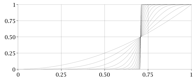
Figure 1: The volume ratio (8) as function of $0\leq\delta<1$ for $m=2^{k}$, $k=1,\ldots,16$, and $n=2m$

If the difference $n-m$ of the dimensions is odd, the arguments from the proof of Theorem 3.3 lead to a representation with an integral remainder that can, however, in the given context almost always be neglected.

Theorem 3.5.

If the difference $n-m\geq 3$ of the two dimensions is odd, if the quantities $k$ and $l$ are defined as in the previous theorem, and if $\nu=k-1/2$ is set,

(9) $$\psi\bigg{(}\frac{\delta}{\sqrt{1-\delta^{2}}}\bigg{)}=\;\sum_{j=0}^{\nu}\,\frac{\Gamma(k+l+1)}{\Gamma(k-j+1)\Gamma(l+j+1)}\,(1-\delta^{2})^{k-j}\,\delta^{2(l+j)}+\Delta(\delta)$$

holds, where the remainder possesses the integral representation

(10) $$\Delta(\delta)=\frac{2}{\sqrt{\pi}}\frac{\Gamma(n/2)}{\Gamma((n-1)/2)}\int_{0}^{\delta}\frac{t^{n-2}}{\sqrt{1-t^{2}}}\,\mathrm{d}t$$

and satisfies the estimate $0\leq\Delta(\delta)\leq\delta^{n-1}$ on its interval of definition.

Proof 3.6.

By a simple substitution one obtains

$$\frac{\Delta(\delta)}{\delta^{n-1}}=\frac{2}{\sqrt{\pi}}\frac{\Gamma(n/2)}{\Gamma((n-1)/2)}\int_{0}^{1}\frac{t^{n-2}}{\sqrt{1-\delta^{2}t^{2}}}\,\mathrm{d}t\leq\Delta(1).$$

Because of $\Delta(1)=1$, the estimate $\Delta(\delta)\leq\delta^{n-1}$ follows.

4 On the limit behavior for high space dimensions

In this section, we derive bounds for the area ratios (2) and the volume ratios (6), respectively, with the aim to understand their behavior when the dimensions tend to infinity. The starting point is a result on general matrices. Its proof is based on the Markov inequality and once again on the separability of Gauss functions.

Theorem 4.1.

Let $0<\sigma_{1}\leq\sigma_{2}\leq\cdots\leq\sigma_{m}$ be the singular values of the matrix $A$ under consideration. The volume ratio (6) can then be estimated as

(1) $$\frac{\lambda\big{(}\big{\{}x\,\big{|}\,\|Ax\|<\delta\,\|A\|\|x\|,\,\|x\|\leq R\big{\}}\big{)}}{\lambda\big{(}\big{\{}x\,\big{|}\,\|x\|\leq R\big{\}}\big{)}}\leq\min_{t}X(t)$$

by the minimum of the strictly convex function

(2) $$X(t)=\bigg{(}\,\prod_{k=1}^{m}\frac{1}{1-\delta^{2}\sigma_{m}^{2}\,t+\sigma_{k}^{2}\,t}\bigg{)}^{1/2}\bigg{(}\frac{1}{1-\delta^{2}\sigma_{m}^{2}\,t}\bigg{)}^{(n-m)/2}$$

over its interval $0\leq t<1/(\delta^{2}\sigma_{m}^{2})$ of definition.

Proof 4.2.

We can restrict ourselves by Lemma 2.4 as before again to the diagonal matrix $\Sigma$ with the entries $\sigma_{1},\ldots,\sigma_{m}$. The characteristic function $\chi$ of the set of all $x$ for which $\|\Sigma x\|<\delta\,\|\Sigma\|\|x\|$ holds satisfies, for any $t>0$, the crucial estimate

$$\chi(x)<\exp\big{(}\,t\,\big{(}\delta^{2}\|\Sigma\|^{2}\|x\|^{2}-\|\Sigma x\|^{2}\big{)}\big{)}$$

by a product of univariate functions. By Lemma 2.1, the subsequent remark, and Lemma 2.3, the volume ratio (7) can therefore be estimated by the integral

$$\Big{(}\frac{1}{\sqrt{\pi}}\Big{)}^{n}\!\int\exp\big{(}\,t\,\big{(}\delta^{2}\|\Sigma\|^{2}\|x\|^{2}-\|\Sigma x\|^{2}\big{)}\big{)}\exp\big{(}-\|x\|^{2}\big{)}\,\mathrm{d}x$$

that remains finite for all $t$ in the given interval. It splits into a product of one-dimensional integrals and takes, for given $t$, the value $X(t)$. All even-order order derivatives of the function $X(t)$ are greater than zero, as follows by differentiation under the integral sign. The function is therefore, in particular, strictly convex.

Because the second-order derivative of $X(t)$ is greater than zero and $X^{\prime}(t)$ tends to infinity as $t$ approaches the right endpoint of the interval, the first-order derivative of the function $X(t)$ possesses a then also unique zero $t^{*}>0$ if and only if

(3) $$X^{\prime}(0)=\frac{n}{2}\,\delta^{2}\sigma_{m}^{2}-\frac{1}{2}\sum_{k=1}^{m}\sigma_{k}^{2}$$

is less than zero, or equivalently if $\delta$ satisfies the condition

(4) $$\bar{\kappa}\delta<\sqrt{\frac{m}{n}},\quad\frac{1}{\bar{\kappa}^{2}}=\frac{1}{m}\sum_{k=1}^{m}\Big{(}\frac{\sigma_{k}}{\sigma_{m}}\Big{)}^{2}.$$

The strictly convex function $X(t)$ attains then and only then its minimum at a point in the interior of the interval and there then takes a value less than $X(0)=1$. Otherwise, the estimate (1) is worthless and $X(t)\geq 1$ for all $t$ in the interval.

The minimum of the function (2) can in general only be calculated numerically, say by some variant of Newton’s method, and cannot be given in closed form. It is, however, comparatively simple to estimate this minimum from above and below.

Lemma 4.3.

Let $\kappa=\sigma_{m}/\sigma_{1}$ again be the condition number of the matrix and let $\xi$ be the square root of the dimension ratio $m/n$. If $\kappa\delta<\xi$, then the estimate

(5) $$\min_{t}X(t)\leq\bigg{(}\,\frac{\kappa\delta}{\xi}\,\bigg{(}\frac{1-\kappa^{2}\delta^{2}}{1-\xi^{2}}\bigg{)}^{\gamma}\;\bigg{)}^{m},\quad\gamma=\frac{1-\xi^{2}}{2\xi^{2}},$$

holds for the minimum of the function (2). Under the for condition numbers $\kappa>1$ weaker condition (4), conversely the lower estimate

(6) $$\min_{t}X(t)\geq\bigg{(}\,\frac{\bar{\kappa}\delta}{\xi}\,\bigg{(}\frac{1-\bar{\kappa}^{2}\delta^{2}}{1-\xi^{2}}\bigg{)}^{\gamma}\;\bigg{)}^{m}$$

holds. For orthogonal projections, in both cases equality holds and it is

(7) $$\min_{t}X(t)=\bigg{(}\,\frac{\delta}{\xi}\,\bigg{(}\frac{1-\delta^{2}}{1-\xi^{2}}\bigg{)}^{\gamma}\;\bigg{)}^{m}.$$

Proof 4.4.

The function (2) reads in the case of orthogonal projections, that is, if all singular values of the matrix take the value $\sigma_{k}=1$, as

$$X(t)=\bigg{(}\frac{1}{1-\delta^{2}t+t}\bigg{)}^{m/2}\bigg{(}\frac{1}{1-\delta^{2}t}\bigg{)}^{(n-m)/2}.$$

It attains its minimum at the point

$$t=\frac{\xi^{2}-\delta^{2}}{(1-\delta^{2})\delta^{2}}$$

in its interval $0<t<1/\delta^{2}$ of definition and takes there the value (7). In the general case, the function (2) satisfies, because of $\sigma_{1}\leq\sigma_{k}$, the estimate

$$X(t)\,\leq\,\bigg{(}\frac{1}{1-\delta^{2}\sigma_{m}^{2}\,t+\sigma_{1}^{2}\,t}\bigg{)}^{m/2}\bigg{(}\frac{1}{1-\delta^{2}\sigma_{m}^{2}\,t}\bigg{)}^{(n-m)/2}.$$

The upper estimate (5) thus follows minimizing the right-hand side as above as a function of $t^{\prime}=\sigma_{1}^{2}\,t$. The proof of the lower estimate is a little bit more involved. Since the geometric mean can be estimated by the arithmetic mean,

$$\bigg{(}\,\prod_{k=1}^{m}\big{(}1-\delta^{2}\sigma_{m}^{2}\,t+\sigma_{k}^{2}\,t\big{)}\bigg{)}^{1/m}\!\leq\;\frac{1}{m}\sum_{k=1}^{m}\big{(}1-\delta^{2}\sigma_{m}^{2}\,t+\sigma_{k}^{2}\,t\big{)}$$

holds. By the definition (4) of $\bar{\kappa}$, this leads to the estimate

$$X(t)\,\geq\,\bigg{(}\frac{1}{1-\delta^{2}\sigma_{m}^{2}\,t+\bar{\kappa}^{-2}\sigma_{m}^{2}\,t}\bigg{)}^{m/2}\bigg{(}\frac{1}{1-\delta^{2}\sigma_{m}^{2}\,t}\bigg{)}^{(n-m)/2}.$$

Minimizing the right-hand side as a function of $t^{\prime}=\bar{\kappa}^{-2}\sigma_{m}^{2}\,t$, one gets (6).

The question is how tight the derived inclusion for the minimum of the function (2) is in nontrivial cases, for condition numbers $\kappa>1$. The answer is that there is practically no room for improvement without additional conditions to the singular values. Consider a sequence of matrices with fixed dimension ratios $\xi^{2}=m/n$ and fixed condition number $\kappa$ and let $\kappa\delta<\xi$. Assume that $\bar{\kappa}$ tends to $\kappa$ as $m$ goes to infinity. This is, for example, the case if $\sigma_{k}=\sigma_{1}$ for $k=1,\ldots,m-1$. The rates

(8) $$\frac{\bar{\kappa}\delta}{\xi}\,\bigg{(}\frac{1-\bar{\kappa}^{2}\delta^{2}}{1-\xi^{2}}\bigg{)}^{\gamma},\quad\frac{\kappa\delta}{\xi}\,\bigg{(}\frac{1-\kappa^{2}\delta^{2}}{1-\xi^{2}}\bigg{)}^{\gamma}$$

then approach each other arbitrarily as $m$ goes to infinity. If additionally

(9) $$\bar{\kappa}=\kappa-\frac{\kappa_{1}}{m}+o\Big{(}\frac{1}{m}\Big{)}$$

holds with some positive constant $\kappa_{1}$, the ratio of the two bounds enclosing the minimum of the function (2) tends to a limit value greater than zero.

The bound (5) can be simplified, and the minimum of the function (2) be further estimated in terms of the function

(10) $$\phi(\vartheta)=\vartheta\,\exp\bigg{(}\frac{1-\vartheta^{2}}{2}\bigg{)},$$

which increases on the interval $0\leq\vartheta\leq 1$ strictly, attains at the point $\vartheta=1$ its maximum value one, and decreases from there again strictly.

Lemma 4.5.

As long as $\kappa\delta$ is less than the square root $\xi$ of $m/n$, one has

(11) $$\min_{t}X(t)\leq\phi\bigg{(}\frac{\kappa\delta}{\xi}\bigg{)}^{m}.$$

Proof 4.6.

Set $\kappa\delta/\xi=\vartheta$ for abbreviation. The logarithm

$$\ln\bigg{(}\bigg{(}\frac{1-\kappa^{2}\delta^{2}}{1-\xi^{2}}\bigg{)}^{\gamma}\;\bigg{)}=\,\frac{1-\xi^{2}}{2\xi^{2}}\,\ln\bigg{(}\frac{1-\vartheta^{2}\xi^{2}}{1-\xi^{2}}\bigg{)}$$

then possesses, because of $\vartheta^{2}\xi^{2}<1$ and $\xi^{2}<1$, the power series expansion

$$\frac{1-\vartheta^{2}}{2}-\frac{1}{2}\,\sum_{k=1}^{\infty}\bigg{(}\frac{1-\vartheta^{2k}}{k}-\,\frac{1-\vartheta^{2k+2}}{k+1}\bigg{)}\xi^{2k}.$$

Because the series coefficients are for all $\vartheta\geq 0$ greater than or equal to zero and, by the way, polynomial multiples of $(1-\vartheta^{2})^{2}$, the proposition follows from (5).

In the following, we will use the estimate (11) for the minimum of the function given by (2). The next theorem is then a trivial conclusion from Theorem 4.1.

Theorem 4.7.

Let $n>m$, let $A$ be an $(m\times n)$-matrix of full rank $m$, let $\kappa$ be the condition number of $A$, and let $\xi$ be the square root of the dimension ratio $m/n$. If $\kappa\delta$ is less than $\xi$, then for all radii $R>0$ one has

(12) $$\frac{\lambda\big{(}\big{\{}x\,\big{|}\,\|Ax\|<\delta\,\|A\|\|x\|,\,\|x\|\leq R\big{\}}\big{)}}{\lambda\big{(}\big{\{}x\,\big{|}\,\|x\|\leq R\big{\}}\big{)}}\leq\phi\bigg{(}\frac{\kappa\delta}{\xi}\bigg{)}^{m}.$$

Consider a sequence of matrices with dimension ratios $m/n\geq\delta_{0}^{2}$ and condition numbers $\kappa\leq\kappa_{0}$. The volume ratios (6) tend then for $\kappa_{0}\delta<\delta_{0}$ not slower than

(13) $$\sim\,\phi\bigg{(}\frac{\kappa_{0}\delta}{\delta_{0}}\bigg{)}^{m}$$

to zero as the dimensions go to infinity. Under suitable conditions to the singular values, considerable improvements are possible. In extreme cases, such as in Lemma 2.12, the volume ratios (6) can essentially be estimated as those for orthogonal projections and the potentially devastating influence of the condition number vanishes.

Theorem 4.8.

Let $n>m$ and let $A$ be a nonvanishing $(m\times n)$-matrix with singular values $\sigma_{k}=\sigma_{m}$ for $k>m_{0}$. If one sets $m^{\prime}=m-m_{0}$ and $\xi^{\prime}$ is the square root of $m^{\prime}/n$, the volume ratio (6) satisfies then for $0\leq\delta<\xi^{\prime}$ the estimate

(14) $$\frac{\lambda\big{(}\big{\{}x\,\big{|}\,\|Ax\|<\delta\,\|A\|\|x\|,\,\|x\|\leq R\big{\}}\big{)}}{\lambda\big{(}\big{\{}x\,\big{|}\,\|x\|\leq R\big{\}}\big{)}}\leq\phi\bigg{(}\frac{\delta}{\xi^{\prime}}\bigg{)}^{m^{\prime}}.$$

The proof results from Lemma 2.12, Theorem 4.1, and Lemma 4.5.

Theorem 4.7 possesses a counterpart that deals with values $\delta$ greater than the square root of the ratio of the dimensions $m$ and $n$.

Theorem 4.9.

Let $A$ be a nonvanishing $(m\times n)$-matrix and let $\xi$ be the square root of the dimension ratio $m/n$. For $\xi<\delta\leq 1$ then one has

(15) $$\frac{\lambda\big{(}\big{\{}x\,\big{|}\,\|Ax\|\geq\delta\,\|A\|\|x\|,\,\|x\|\leq R\big{\}}\big{)}}{\lambda\big{(}\big{\{}x\,\big{|}\,\|x\|\leq R\big{\}}\big{)}}\leq\phi\bigg{(}\frac{\delta}{\xi}\bigg{)}^{m}.$$

Proof 4.10.

We can restrict ourselves again to diagonal matrices $A=\Sigma$. Let $P$ be the matrix that extracts from a vector in $\mathbb{R}^{n}$ its first $m$ components. As $\|\Sigma x\|\leq\|\Sigma\|\|Px\|$ and $\|\Sigma\|>0$, the given volume ratio can then be estimated by the volume ratio

$$\frac{\lambda\big{(}\big{\{}x\,\big{|}\,\|Px\|\geq\delta\,\|x\|,\,\|x\|\leq R\big{\}}\big{)}}{\lambda\big{(}\big{\{}x\,\big{|}\,\|x\|\leq R\big{\}}\big{)}}.$$

As in the proof of Theorem 4.1, we can estimate this volume ratio for sufficiently small positive values $t$ by the integral

$$\Big{(}\frac{1}{\sqrt{\pi}}\Big{)}^{n}\!\int\exp\big{(}\,t\,\big{(}\|Px\|^{2}-\delta^{2}\|x\|^{2}\big{)}\big{)}\exp\big{(}-\|x\|^{2}\big{)}\,\mathrm{d}x.$$

This integral splits into a product of one-dimensional integrals and takes the value

$$\bigg{(}\frac{1}{1+\delta^{2}t-t}\bigg{)}^{m/2}\bigg{(}\frac{1}{1+\delta^{2}t}\bigg{)}^{(n-m)/2},$$

which attains, for $\delta<1$, on the interval $0<t<1/(1-\delta^{2})$ its minimum at

$$t=\frac{\delta^{2}-\xi^{2}}{(1-\delta^{2})\delta^{2}}.$$

It takes at this point $t$ again the value

$$\bigg{(}\,\frac{\delta}{\xi}\,\bigg{(}\frac{1-\delta^{2}}{1-\xi^{2}}\bigg{)}^{\gamma}\;\bigg{)}^{m},\quad\gamma=\frac{1-\xi^{2}}{2\xi^{2}}.$$

This leads as in the proof of Lemma 4.5 to the estimate (15). As the set of all $x$ for which $\|Px\|=\|x\|$ holds has measure zero, (15) remains true for $\delta=1$.

For $(m\times n)$-matrices $A$ with dimension ratio $m/n\leq\delta_{0}^{2}$, the volume ratios (6) tend therefore on the interval $\delta_{0}<\delta\leq 1$ pointwise and on its closed subintervals uniformly and exponentially to one as $m$ goes to infinity. For sequences of matrices for which the ratio $m/n$ of their dimensions tends to zero, the volume ratios (6) hence tend, for all $\delta>0$, pointwise to one. This has, however, often less severe implications than it might first appear. This is demonstrated by the example of the matrices $A=T^{t}$ from section 2, whose dimensions (13) were

(16) $$m=3\times N,\quad n=3\times\frac{N(N+1)}{2}.$$

Figure 2 shows the bounds for the volume ratios (6) resulting from the application of Lemma 2.12 to these matrices as functions of $\delta<1$ for $N$ ranging from $4$ to $32$, or, in the framework of quantum mechanics, for systems with up to $32$ electrons.

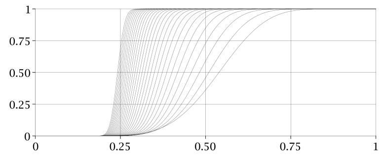
Figure 2: The bounds for the volume ratios (6) for the example from section 2 for $N=4,\ldots,32$.

We finally consider the case of orthogonal projections from the $\mathbb{R}^{n}$ to the $\mathbb{R}^{m}$, that is, of $(m\times n)$-matrices $P$ with one as the only singular value. The condition number of such matrices is $\kappa=1$, and their norm is $\|P\|=1$. If the dimension ratios $m/n$ tend to $\delta_{0}^{2}$, or even remain as in Figure 1 fixed, the corresponding volume ratios (8) tend therefore to a step function with jump discontinuity at $\delta_{0}$. This observation is widely equivalent to the random projection theorem. Let $\xi$ be again the square root of $m/n$. For a randomly chosen vector $x$, the probability that

(17) $$(1-\varepsilon)\xi\,\|x\|\leq\|Px\|<(1+\varepsilon)\xi\,\|x\|$$

holds is then $F((1+\varepsilon)\xi)-F((1-\varepsilon)\xi)$, with the at least for even-numbered differences of the dimensions explicitly known distribution function

(18) $$F(\delta)=\psi\bigg{(}\frac{\delta}{\sqrt{1-\delta^{2}}}\bigg{)},$$

and tends exponentially to one as $m$ goes to infinity. This means that the orthogonal projection of a randomly chosen unit vector $x\in\mathbb{R}^{n}$ onto a given subspace of high dimension $m$ possesses with high probability a norm

(19) $$\approx\sqrt{\frac{m}{n}}.$$

A lower bound for this probability depending only on the dimension $m$ but not on the dimension $n$ can be derived from the estimates (12) and (15). Because of

(20) $$\phi(1\pm\varepsilon)<\exp(-c\,\varepsilon^{2}),\quad c=-\ln(\phi(2)),$$

for values $0<\varepsilon<1$, the probability that (17) holds is in any case greater than

(21) $$1-2\exp(-c\,\varepsilon^{2}m)$$

and the random projection theorem recovered.

References

[1]A. E. Brouwer and W. H. Haemers, Spectra of Graphs, Springer, New
York, 2012.
[2]D. Cvetković, P. Rowlinson, and S. Simić, An Introduction to
the Theory of Graph Spectra, Cambridge University Press, Cambridge, UK,
2010.
[3]A. Edelman, Eigenvalues and Condition Numbers of Random Matrices,
PhD thesis, Massachusetts Institute of Technology, Cambridge, MA, 1989.
[4]S. Foucart and H. Rauhut, A Mathematical Introduction to Compressive
Sensing, Birkhäuser/Springer, New York, 2013.
[6]W. B. Johnson and J. Lindenstrauss, Extensions of Lipschitz
mappings into a Hilbert space, in Conference in Modern Analysis and
Probability, Contemp. Math. 26, AMS, Providence, RI, 1984, pp. 189–206.
[7]M. Ledoux, The Concentration of Measure Phenomenon, AMS,
Providence, RI, 2001.
[8]M. Ledoux and M. Talagrand, Probability in Banach Spaces, Springer,
Berlin, 1991.
[9]G. V. Livshyts, K. Tikhomirov, and R. Vershynin, The smallest
singular value of inhomogeneous square random matrices, The Ann. Probab., 49
(2021), pp. 1286–1309.
[10]G. G. Lorentz, Bernstein Polynomials, Chelsea, New York, 1986.
[11]M. Rudelson and R. Vershynin, The smallest singular value of a
random rectangular matrix, Comm. Pure Appl. Math., 62 (2009),
pp. 1707–1739.
[12]T. Tao and V. Vu, Random matrices: The distribution of the smallest
singular values, Geom. Funct. Anal., 20 (2010), pp. 260–297.
[13]R. Vershynin, High-Dimensional Probability, Cambridge University
Press, Cambridge, UK, 2018.
[14]H. Yserentant, On the expansion of solutions of Laplace-like
equations into traces of separable higher-dimensional functions, Numer.
Math., 146 (2020), pp. 219–238.