Parrondo’s paradox for homeomorphisms

Abstract.

We construct two planar homeomorphisms $f$ and $g$ for which the origin is a globally asymptotically stable fixed point whereas for $f\circ g$ and $g\circ f$ the origin is a global repeller. Furthermore, the origin remains a global repeller for the iterated function system generated by $f$ and $g$ where each of the maps appears with a certain probability. This planar construction is also extended to any dimension greater than 2 and proves for first time the appearance of the Parrondo’s dynamical paradox in odd dimensions.

Mathematics Subject Classification 2010: 37C25, 37C75, 37H05.

Keywords: Fixed points, Local and global asymptotic stability, Parrondo’s dynamical paradox, Random dynamical system.

1. Introduction and main results

The Parrondo’s paradox is a well-known paradox in game theory, that in a few words affirms that a combination of losing strategies can become a winning strategy, see [9, 11]. In the dynamical context, when we study the stability of fixed points, the role of being a winning or a losing strategy can be replaced by being an attracting or repelling fixed point. A word of caution, throughout this note we use the term attracting (or attractor) and repelling (or repeller) as a synonym of asymptotically stable for a map and its inverse, respectively. Hence, for a fixed class of maps $\mathcal{C},$ from $\mathbb{R}^{k}$ into itself, we will say that a pair of maps $f,g\in\mathcal{C}$ exhibit a dynamical Parrondo’s paradox if they have a common fixed point at which the maps are locally invertible and the fixed point is locally asymptotically stable for $f$ and $g$ but it is a repeller for the composite maps $g\circ f$ and $f\circ g.$ Notice that, $g\circ f$ and $f\circ g$ are conjugate near the fixed point because, locally, $f\circ g=g^{-1}\circ g\circ f\circ g.$

As shown in [5], the dynamical Parrondo’s paradox can arise when $k$ is even and $\mathcal{C}$ is the class of polynomial maps. On the contrary, it is also proved in [5] that the paradox does not appear when $k=1$ and $\mathcal{C}$ is the class of analytic maps. Notice also that the paradox is also impossible for any $k$ when $\mathcal{C}$ is the class of maps for which the common fixed point is hyperbolic. Indeed, given two $k\times k$ matrices with all their eigenvalues with modulus smaller than 1, $A$ and $B$, it holds that $|\mathrm{det}(A)|<1,|\mathrm{det}(B)|<1$ and hence $|\mathrm{det}(AB)|<1$. As a consequence, when two maps share a common fixed point ${\bf x}$ which is asymptotically stable for both of them and the maps are of class $\mathcal{C}^{1}$ at ${\bf x},$ then, generically, for $g\circ f$ and $f\circ g$ the fixed point ${\bf x}$ is, in both cases, either locally asymptotically stable or of saddle type, but it can never be repeller. Examples of saddle type points for $g\circ f,$ when $f$ and $g$ are linear maps, are given in [3] and [10, p. 8].

For the sake of completeness, and to compare it with our result, we recall the example in [5, Ex. 7] for $k=2,$

$$f(x,y) =\big{(}-y+2{x}^{2}+6xy,x-3{x}^{2}+2xy+3{y}^{2}\big{)},$$

$$g(x,y) =\big{(}{x}/{2}-{\sqrt{3}}y/{2}-x\,(x^{2}+y^{2}),{\sqrt{3}}x/{2}+{y}/{2}-y\,(x^{2}+y^{2})\big{)}.$$

It can be proved that the origin is a locally asymptotic stable fixed point for $f$ and $g$ and the origin is a repelling fixed point for $g\circ f$ by computing the so called Birkhoff stability constants for the three maps. Notice that the dynamics near the fixed points is of rotation type. Taking the product of these maps $j$ times with themselves we trivially obtain examples of pairs of maps exhibiting the dynamical Parrondo’s paradox for all $k=2j.$

It is worth to mention that in [4] a different type of dynamical Parrondo’s paradox is considered. The authors combine periodically two 1-dimensional maps $f$ and $g$ to give rise to chaos or order.

The main goal of this paper is to give examples of the dynamical Parrondo’s paradox when $\mathcal{C}$ is the class of homeomorphisms and to fill the the lack of examples in odd dimension. We prove that for all $k\geq 2$ there are pairs of maps that realize the dynamical Parrondo’s paradox. While the approach of [5] is mainly analytic, our point of view is more qualitative. Moreover, the behaviour of our maps near the fixed point is not of rotation type and there does not seem to be a clear path to make them smooth or analytic.

Theorem 1.

For any $k\geq 2$, there are pairs of homeomorphisms from $\mathbb{R}^{k}$ to itself that exhibit the dynamical Parrondo’s paradox. However, for $k=1$ the paradox never arises.

It is interesting to remark that Theorem 1, and in consequence, the dynamical Parrondo’s paradox is also relevant from the point of view of 2-periodic discrete dynamical systems. In particular, these systems are good models for describing the dynamics of biological systems under periodic fluctuations due either to external disturbances or effects of seasonality, see [6, 7, 8, 12, 13] and the references therein.

As a byproduct of our construction of the 2-dimensional example of dynamical Parrondo’s paradox we will also prove that, almost surely, every orbit of the iterated function system generated by $f$ and $g$ is repelled from the origin, where $f$ and $g$ are essentially the maps constructed in Theorem 1 and appear with certain respective probabilities $p$ and $1-p$. The result carries onto higher dimensions as well. To be more precise, consider the space $\{0,1\}^{\mathbb{N}}$ equipped with the probability measure $\mu$ defined as the product of the Bernoulli probability measures, $\mu_{B},$ in each factor. Recall that for the Bernoulli distribution $\operatorname{B}(p),$ $\mu_{B}(1)=p$ and $\mu_{B}(0)=q=1-p,$ for some $p\in[0,1].$ We prove:

Theorem 2.

For any $k\geq 2$ and $0<p<1,$ there exist homeomorphisms $f_{0}$ and $f_{1}$ from $\mathbb{R}^{k}$ into itself such that:

• The origin is fixed and globally asymptotically stable for $f_{0}$ and $f_{1}$.

• For ${\bf 0}\neq{\bf x}\in\mathbb{R}^{k}$ and for $\mu$-almost all $(a_{n})\in\{0,1\}^{\mathbb{N}}$ the orbit $\{F_{a_{n},\cdots,a_{1},a_{0}}({\bf x})\}_{n\geq 1}$ is repelled from the origin, where $F_{a_{n},\cdots,a_{1},a_{0}}=f_{a_{n}}\circ\ldots\circ f_{a_{1}}\circ f_{a_{0}},$ for $n\geq 1,$ $f_{0}$ appears with probability $p$ and $f_{1}$ with probability $1-p.$

As we will see in the proof, for any $0<p<1,$ each homomorphism $f_{0}$ and $f_{1}$ will have a region where the radial component of the points increases and another one where it decreases. The largest of these variations corresponds to the increasing region, which is in turn considerably bigger in size than the decreasing region. Their difference becomes larger and tends to infinity when $p$ approaches 0 or 1.

2. Definition of $f$ and $g$ and proof of Theorem 1

We will split the proof in three cases: $k=1,$ $k=2$ and $k>2.$

2.1. Proof of Theorem 1 for $k=1$

Let us proceed by contradiction. Suppose that $f$ and $g$ are homeomorphisms of $\mathbb{R}$, $0$ is a locally attracting fixed point for $f$ and $g$ and a locally repelling fixed point for $f\circ g$ and $g\circ f$. Assume further, for simplicity, that $f$ and $g$ reverse orientation, the other cases are handled similarly. Then:

• $g$ is monotone decreasing, so if $y<x<0$ then $0<g(x)<g(y)$.

• Since $0$ is locally attracting for $f$ and $g$, for any $y<0<x$ close to $0$ we have that

  $y<f\circ f(y)<0<g\circ g(x)<x$.

• Since $0$ is locally repelling for $f\circ g$ and $g\circ f$, for any $x,y>0$ close to $0$ we have that

  $x<f\circ g(x)$  and  $y<g\circ f(y)$.

These properties put together yield a contradiction because for small positive $u>0$:

$u<f\circ g(u)<g\circ f(f\circ g(u))=g(f\circ f(g(u))<g(g(u))<u$

where the first two inequalities are consequence of $(iii)$ and the last two inequalities are consequence $(i)$ and $(ii)$.

However, notice that it is possible to construct an example in which the origin is semistable for $f\circ g$ (and also for $g\circ f$) while it is asymptotically stable for $f$ and $g$:

$$f(x)=\begin{cases}-2x&\text{if }x\leq 0,\\ -x/3&\text{if }x\geq 0,\end{cases}\enskip\enskip\enskip\enskip g(x)=\begin{cases}-x/3&\text{if }x\leq 0,\\ -2x&\text{if }x\geq 0.\end{cases}\enskip\enskip\Rightarrow\enskip\enskip f\circ g(x)=\begin{cases}x/9&\text{if }x\leq 0,\\ 4x&\text{if }x\geq 0.\end{cases}$$

2.2. Proof of Theorem 1 for $k=2$

In our example the maps $f$ and $g$ are conjugate. We first focus on the definition of $f$, expressed in polar coordinates. The first elements of a typical orbit under $f$ will drift away from the origin (the radial coordinate increases) until it reaches a trapping sector in which the orbit remains forever and is slowly attracted to the origin (the radial coordinate steadily decreases). The dynamics of the angular coordinate is independent from the values of the radial coordinate and forces every orbit to be eventually contained in the trapping sector. Note that, globally, $f$ looks mostly expanding because the size of this sector and the speed of convergence to the origin therein are relatively small.

Let us write out the details. Identify $\mathbb{R}^{2}\setminus\{\textbf{0}\}$ with the cylinder $\mathbb{R}\times\mathbb{R}/\mathbb{Z}$ so as to use polar coordinates $(r,\theta)$ where $r\in\mathbb{R}$. The origin corresponds to the lower end ($r=-\infty$) of the cylinder. Notice that this is not the typical range for the radial coordinate but it will later ease our computations. Let $I\subset\mathbb{R}/\mathbb{Z}$ be an interval centered at $\bar{0}$ (here $\bar{0}$ is used to denote the neutral element in $\mathbb{R}/\mathbb{Z}$) and such that $I\cap(I+\overline{1/2})=\emptyset$. Let $f(r,\theta)=(r^{\prime},\theta^{\prime})$ be a homeomorphism of the cylinder that satisfies:

• $\Delta_{r}=r^{\prime}-r$ and $\Delta_{\theta}=\theta^{\prime}-\theta$ only depend on $\theta$.

• $\Delta_{r}=4$ if $\theta\notin I$, $\Delta_{r}\in[-1,0)$ if $\theta$ belongs to an interval $J\subset I$, $\bar{0}\in J$ and equals $-1$ if $\theta=\bar{0}$, see Figure 1.

• $\Delta_{\theta}$ is non-negative, $\Delta_{\theta}\leq\mathrm{dist}(I,I+\overline{1/2})$ and $\Delta_{\theta}=0$ if and only if $\theta=\bar{0}$.

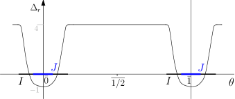
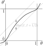
Figure 1. Graphs of $\Delta_{r}$ (left) and $\theta^{\prime}$ (right) as a function of $\theta$ in the definition of $f.$

Property $(iii)$ controls the 1-dimensional dynamics in the angular coordinate: every orbit tends to $\theta=\bar{0}$. By $(ii)$ the radial coordinate decreases indefinitely once the orbit remains close to $\theta=\bar{0}$. From $(i)$ we deduce that $\Delta_{r}$ is uniformly bounded and, as a consequence, $f$ extends to a planar homeomorphism, which we will also denote by $f$, by imposing that the origin is a fixed point $f(\textbf{0})=\textbf{0}$.

The angular interval $J$ determines an infinite cone $\widehat{J}$ in which the radial coordinate of a point decreases after applying $f$. Inside $\widehat{J}$ we find the trapping sector that has been previously mentioned, see Figure 2. Notice also that the speed of attraction ($\Delta_{r}\in[-1,0)$) in the trapping sector is weaker than the speed of repulsion ($\Delta_{r}=4$) outside the cone $\widehat{I}$ determined by $I$.

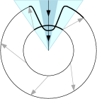
Figure 2. Action of $f$ on a circle $r=c$ (inner circle) represented schematically by arrows, cones $\widehat{I}$ (light) and $\widehat{J}$ (dark) are shadowed, the attracting $f$–invariant ray ($\theta=\bar{0}$) is depicted vertical.

The map $g$ is merely a copy of $f$ shifted in the angular coordinate. Let $\tau(r,\theta)=(r,\theta+\overline{1/2})$ be the half-turn rotation in the plane and let $g=\tau^{-1}\circ f\circ\tau=\tau\circ f\circ\tau$. Being a conjugate of $f$, $g$ satisfies the same properties as $f$ if we replace $\theta$ by $\theta+\overline{1/2}$ in the statements. The key observation is that by the second item in $(iii)$, $f(\widehat{I})\cap\tau(\widehat{I})=\{\textbf{0}\}$ and $g(\tau(\widehat{I}))\cap\widehat{I}=\{\textbf{0}\}$. This means that the radial coordinate cannote decrease under the action of $f$ and then immediately decrease under the action of $g$, or viceversa. In fact, by $(ii)$ the radial coordinate increases after applying $g\circ f$ or $f\circ g$.

Let us finally prove that $f$ and $g$ exhibit the dynamical Parrondo’s paradox.

The origin is a globally attracting fixed point for $f$ and $g$. Let $\{(r_{n},\theta_{n})\}_{n\geq 1}$ be the orbit under $f$ of a point $(r,\theta)$. We study separately the angular coordinate $\{\theta_{n}\}$ because its evolution is independent from the values of the radial coordinate. If $\theta=\bar{0}$ then $\theta_{n}=\bar{0}$ for every $n\geq 1$, otherwise the sequence $\{\theta_{n}\}$ is increasing and converges to the unique value $\theta_{0}$ which is fixed under the 1-dimensional angular dynamics, namely $\theta_{0}=\bar{0}$. Thus, $\theta_{n}\to\bar{0}$ so $\theta_{n}\in J$ for sufficiently large $n$, say $n\geq n_{0}$. This implies that $r_{n+1}<r_{n}$ for every $n\geq n_{0}$ and, additionally, that $r_{n+1}-r_{n}\to-1$ as $n\to+\infty$ because the orbit converges towards the half-ray $\theta=\bar{0}$. As a consequence, $r_{n}\to-\infty$ and the orbit tends to the origin.

The same conclusion holds for $g$ because it is conjugate to $f$.

The origin is a globally repelling fixed point for $f\circ g$ and $g\circ f$. Recall that $f\circ g=f\circ\tau\circ f\circ\tau$ is conjugate to $g\circ f=\tau\circ f\circ\tau\circ f$ (notice that $\tau^{2}=\mathrm{id}$) so it is enough to prove the statement for the latter composition. By $(ii)$ the radial coordinate of a point outside $\widehat{I}$ increases by 4 under the action of $f$. Thus, if $(r^{\prime},\theta^{\prime})=g\circ f(r,\theta)$ we have that $r^{\prime}-r\geq 3$ if $\theta\notin I$. The same inequality is true in the case $f(r,\theta)$ does not belong to $\tau(\widehat{I})$. Since $\widehat{I}\cap f^{-1}(\tau(\widehat{I}))=\{\textbf{0}\}$ we conclude that the radial coordinate of every point increases at least by 3 after applying $g\circ f$. Evidently, the origin is a global repeller for $g\circ f$ and the proof of Theorem 1 follows for $k=2.$

2.3. Proof of Theorem 1 for $k>2$

First, let us modify slightly the planar dynamics introduced in the previous subsection in order to make it symmetric with respect to the vertical axis. Define $h(r,\theta)=f(r,2\theta)$ if $\theta\in[\bar{0},\overline{1/2}]$ and $h(r,\theta)=f(r,1-2\theta)$ if $\theta\in[\overline{1/2},\bar{1}]$. There are now two invariant rays for $h$, $\theta=\bar{0}$, which acts as a repeller in the dynamics in the angular coordinate, and $\theta=\overline{1/2}$, which acts as an attractor. The dynamics of $h$ within each half-plane reproduces the dynamics of $f$ except from the fact that both $h$-invariant rays correspond to the unique invariant ray $\{\theta=\bar{0}\}$ for $f$.

Now, it is straightforward to move into higher dimensions. Consider spherical coordinates $(r,\theta,\varphi_{1},\ldots,\varphi_{k-2})$ in $\mathbb{R}^{k}$ and define a map $h_{k}\colon\mathbb{R}^{k}\to\mathbb{R}^{k}$ by the transformation that applies $h$ to the radial and polar coordinate, $(r^{\prime},\theta^{\prime})=h(r,\theta)$, and leaves the azimuthal coordinates unchanged, $(\varphi^{\prime}_{1},\ldots,\varphi^{\prime}_{k-2})=(\varphi_{1},\ldots,\varphi_{k-2})$. The dynamics of $h_{k}$ leaves invariant the two rays that form the vertical axis (north-south direction, suppose that north corresponds to $\theta=\bar{0}$). Points are attracted to the origin in those rays. Moreover, the radial coordinate of any point increases significantly after applying $h_{k}$ unless the point belongs to a thin double cone $C$ around the axis (whose size can be traced back to the size of $I$). Nevertheless, since every orbit either belongs to the ray pointing to the north or eventually enters the cone around the ray that points to the south and remains in it, we conclude that the origin is a globally attracting fixed point for $h_{k}$.

An analogous construction for the second map as in the case $k=2$ works here as well. Let $\tau_{k}$ be a $90^{o}$-degree rotation in $\mathbb{R}^{k}$ and define $j_{k}=\tau_{k}^{-1}\circ h_{k}\circ\tau_{k}$. Note that

($\star$)   $h_{k}(C)\cap\tau_{k}(C)=\{\textbf{0}\}$  and  $j_{k}(\tau_{k}(C))\cap C=\{\textbf{0}\}$

It is straightforward to check that the origin is a globally attracting fixed point for $j_{k}$ (again by conjugation) and that the radial coordinate of every point increases under the action of $j_{k}\circ h_{k}$ and $h_{k}\circ j_{k}$ (by ($\star$)) and the origin is a globally repelling fixed point for the composite maps.

3. Iterated function system: proof of Theorem 2

The idea is to take as $f_{0}$ and $f_{1}$ a slight modification of the maps $f$ and $g$ defined in the proof of Theorem 1. For the sake of clarity, we only discuss the case $k=2$, the proof for $k>2$ is a straightforward generalization of the argument using the maps $h_{k}$ and $j_{k}$.

Let us start with the proof of Theorem 2 for $k=2$. We need to slightly modify the definition of $f$ and $g$ in Subsection 2.2 in order to increase the rate of radial repulsion far from the invariant rays to account for the effect of the probability $p$. The only change in the definition of the new $f$, which we shall denote in the following by $f_{0}$, is that we replace property $(ii)$ by

• $\Delta_{r}=a-1,$ for some fixed $a>4,$ to be determined later, if $\theta\notin I$, $\Delta_{r}\in[-1,0)$ if $\theta$ belongs to an interval $J\subset I$, $\bar{0}\in J$ and equals $-1$ if $\theta=\bar{0}$.

Then, the new $g$, which shall be henceforth denoted $f_{1}$, is constructed from the new $f$ as in the previous section, $f_{1}=\tau^{-1}\circ f_{0}\circ\tau$. Notice that the original $f$ and $g$ considered in Subsection 2.2 correspond to $a=5.$ The value $a$ will be fixed later, in terms of $p.$

Take an arbitrary point ${\bf x}$ in the plane, different from the origin, and apply $f_{0}$ and $f_{1}$ randomly as in the statement, that is, apply $f_{0}$ with probability $p$ and $f_{1}$ with probability $q=1-p.$ We claim that the orbit of ${\bf x}$ is repelled from the origin almost surely, that is, with probability 1.

The proof of the claim follows from two remarks. The first one concerns the four maps $f_{0}\circ f_{0},f_{0}\circ f_{1},f_{1}\circ f_{0},f_{1}\circ f_{1}$. Their radial coordinate change is bounded by:

$$\Delta_{r}^{f_{0}\circ f_{0}}\geq-2,\quad\Delta_{r}^{f_{0}\circ f_{1}}\geq a-2,\quad\Delta_{r}^{f_{1}\circ f_{0}}\geq a-2\quad\mbox{and}\quad\Delta_{r}^{f_{1}\circ f_{1}}\geq-2.$$

Moreover, the map $f_{0}\circ f_{0}$ appears with probability $p^{2},$ the map $f_{1}\circ f_{1}$ with probability $q^{2},$ while each of the maps $f_{0}\circ f_{1}$ and $f_{1}\circ f_{0}$ appears with probability $pq.$ Let us start giving conditions on $a$ that imply that the expected value of the change in radial coordinate is positive. More precisely, if $\Delta^{n}$ denotes the random variable that measures the minimum of the variation of radial coordinate between a point (different from the origin) and its image under $F_{a_{n},\cdots,a_{1},a_{0}}$ we have that

$$E[\Delta^{2m+2}] \geq E[\Delta^{2m}]+p^{2}\min\Delta_{r}^{f_{0}\circ f_{0}}+pq\min\Delta_{r}^{f_{0}\circ f_{1}}+pq\min\Delta_{r}^{f_{1}\circ f_{0}}+q^{2}\min\Delta_{r}^{f_{1}\circ f_{1}}$$

$$\geq E[\Delta^{2m}]+2(a-2)pq-2(p^{2}+q^{2})=E[\Delta^{2m}]+2\big{(}ap(1-p)-1\big{)}.$$

Hence, if we take any $a$ such that $ap(1-p)-1>0$ we have that $E[\Delta^{2m+2}]\geq E[\Delta^{2m}]+K,$ for $K=2\big{(}ap(1-p)-1\big{)}>0,$ and as a consequence we conclude that $E[\Delta^{2m}]\geq 2Km$, that is, the expected value of $\Delta^{n}$ grows linearly with $n$. This computation shows that in average random iteration repels points from the origin by increasing (linearly!) its radial coordinate. We need to extend this conclusion to a subset of binary sequences of full probability. Notice incidentally that $a>1/\big{(}p(1-p)\big{)}\geq 4.$

Given a binary sequence $(a_{n})$ we can bound the value of $\Delta^{2m}$ in the following fashion

$$\Delta^{2m}\geq\Delta_{r}^{f_{a_{1}}\circ f_{a_{0}}}+\Delta_{r}^{f_{a_{3}}\circ f_{a_{2}}}+\ldots+\Delta_{r}^{f_{a_{2m}}\circ f_{a_{2m-1}}}\geq(a-2)k_{m}-2(m-k_{m})=ak_{m}-2m,$$

where $k_{n}$ denotes the number of maps among $f_{a_{1}}\circ f_{a_{0}},f_{a_{3}}\circ f_{a_{2}},\ldots,f_{a_{2n}}\circ f_{a_{2n-1}}$ that are equal to $f_{1}\circ f_{0}$ or $f_{0}\circ f_{1}$. Notice that $k_{n}$ is the sum of $n$ independent Bernoulli distributions $\operatorname{B}(2pq),$ because $2pq$ is the probability of appearance of $f_{1}\circ f_{0}$ or $f_{0}\circ f_{1}$. Thus, if $\liminf_{n\to+\infty}k_{n}/n=\ell>2/a$, the asymptotic growth of $\Delta^{2n}$ is bounded from below by $(\ell-2/a)n$. In particular, $\Delta^{2n}\to+\infty$ so every point is repelled from the origin by the iterated action of the maps $f_{a_{n}},n\geq 1$.

It only remains to prove that the subset of $(a_{n})$ such that $\liminf k_{n}/n>2/a$ has full probability. In fact, the Strong Law of Large Numbers ([1, 2]) gives much more: for a full probability set, the previous $\liminf$ is indeed a limit and it coincides with the expected value of the random variable $\operatorname{B}(2pq),$ that is $2pq.$ Hence, for a full probability set of binary sequences,

$$\ell=\liminf_{n\to+\infty}\frac{k_{n}}{n}=\lim_{n\to+\infty}\frac{k_{n}}{n}=2pq=2p(1-p).$$

For those sequences we have that,

$$\ell-\frac{2}{a}=2p(1-p)-\frac{2}{a}=\frac{2\big{(}ap(1-p)-1\big{)}}{a}>0,$$

as we wanted to prove, and the theorem follows.

Acknowledgements

This work has received funding from the Ministerio de Ciencia e Innovación (MTM2016-77278-P FEDER, PGC2018-098321-B-I00 and PID2019-104658GB-I00 grants), the Agència de Gestió d’Ajuts Universitaris i de Recerca (2017 SGR 1617 grant).

References

- [1] R. B. Ash. Real analysis and probability. Probability and Mathematical Statistics, No. 11. Academic Press, New York-London, 1972.
- [2] P. Billingsley. Probability and measure. Third edition. Wiley Series in Probability and Mathematical Statistics. A Wiley-Interscience Publication. John Wiley & Sons, Inc., New York, 1995.
- [3] V. D. Blondel, J. Theys, J. N. Tsitsiklis.When is a pair of matrices stable?. In: V. D. Blondel, A. Megretski (eds.). Unsolved problems in Mathematical Systems and Control Theory. Princeton Univ. Press, NJ 2004.
- [4] J. S. Cánovas, A. Linero, D. Peralta-Salas. Dynamic Parrondo’s paradox. Physica D 218 (2006) 177–184.
- [5] A. Cima, A. Gasull, V. Mañosa. Parrondo’s dynamic paradox for the stability of non-hyperbolic fixed points. Discrete Contin. Dyn. Syst. 38 (2018), 889–904.
- [6] S. Elaydi, R. J. Sacker. Global stability of periodic orbits of non-autonomous difference equations and population biology. J. Differential Equations 208 (2005), 258–273.
- [7] S. Elaydi, R. J. Sacker. Periodic difference equations, population biology and the Cushing-Henson conjectures. Math. Biosci. 201 (2006), 195–207.
- [8] J. E. Franke, J. F. Selgrade. Attractors for discrete periodic dynamical systems. J. Math. Anal. Appl. 286 (2003), 64–79.
- [9] G. P. Harmer and D. Abbott. Losing strategies can win by Parrondo’s paradox. Nature (London), Vol. 402, No. 6764 (1999) p. 864.
- [10] R. Jungers. The Joint Spectral Radius. Spinger, Berlin 2009.
- [11] J. M. R. Parrondo. How to cheat a bad mathematician. in EEC HC&M Network on Complexity and Chaos (#ERBCHRX-CT940546), ISI, Torino, Italy (1996), Unpublished.
- [12] J. F. Selgrade, J. H. Roberds. On the structure of attractors for discrete, periodically forced systems with applications to population models. Physica D 158 (2001), 69–82.
- [13] J. F. Selgrade, J. H. Roberds. Global attractors for a discrete selection model with periodic immigration. J. Difference Equations and Appl. 13 (2007), 275–287.