The role of counterions in ionic liquid crystals

Abstract

Previous theoretical studies of calamitic (i.e., rod-like) ionic liquid crystals (ILCs) based on an effective one-species model led to indications of a novel smectic-A phase with a layer spacing being much larger than the length of the mesogenic (i.e., liquid-crystal forming) ions. In order to rule out the possibility that this wide smectic-A phase is merely an artifact caused by the one-species approximation, we investigate an extension which accounts explicitly for cations and anions in ILCs. Our present findings, obtained by grand canonical Monte Carlo simulations, show that the phase transitions between the isotropic and the smectic-A phases of the cation-anion system are in qualitative agreement with the effective one-species model used in the preceding studies. In particular, for ILCs with mesogenes (i.e., liquid-crystal forming species) carrying charged sites at their tips, the wide smectic-A phase forms, at low temperatures and within an intermediate density range, in between the isotropic and a hexagonal crystal phase. We find that in the ordinary smectic-A phase the spatial distribution of the counterions of the mesogens is approximately uniform, whereas in the wide smectic-A phase the small counterions accumulate in between the smectic layers. Due to this phenomenology the wide smectic-A phase could be interesting for applications which hinge on the presence of conductivity channels for mobile ions.

I Introduction

Ionic liquid crystals (ILCs) are versatile materials which exhibit, on the one hand, properties of ionic systems, such as the capability of charge transport, and, on the other hand, they are able to form mesophases which is the distinctive feature of liquid crystals Binnemans2005 ; Goossens2016 .

Recently, several numerical studies Kondrat2010 ; Saielli2017 ; Bartsch2017 ; Bartsch2019 aimed at gaining insight into the link between the underlying molecular features of ILCs and their resulting properties, like the phase behavior or the formation of nanostructures. The complicated interplay of anisotropy and ionic molecular properties renders ILCs to be challenging objects for theoretical studies. Molecular dynamics (MD) computer simulations can be performed with a rather detailed description of the underlying molecules Saielli2012 . Such simulations can provide a rich and detailed picture of the structures of the formed mesophases. But the complexity of the underlying models makes it still difficult to pinpoint basic characteristics of these systems which give rise to the observed properties (or at least being essential for their appearance).

In this regard, studying simplified models allows one to elucidate the generic interplay of the key features of ILCs. This might provide insight into elementary mechanisms on the molecular level, which are necessary ingredients to the rich phenomenology of ILC systems. The natural drawback of simplistic models is that not all of the observable features are captured. At the same time, one is able to rule out minimal models, which are insufficient to describe (or explain) particular phenomena of the object of interest. Thereby, it is possible to successively approach and isolate the minimal physical requirements for the diverse phenomenology occurring for complex systems such as ILCs. Moreover, this procedure yields a generic understanding of the individual microscopic mechanisms involved in the complex, mesoscopic and macroscropic materials properties.

Typically the mesogenes of ILC systems are composed of long alkyl-chains in combination with charged groups, like imidazolium rings Binnemans2005 . Due to the alkyl chains, ILC molecules exhibit a large aspect ratio, rendering the molecules highly anisotropic in shape. However, due to the flexibility of the molecules the formation of liquid crystalline phases (or mesophases) is not self-evident. Notwithstanding, in the spirit of the aforementioned simplified model descriptions, within the present study we refrain from focussing on the formation of orientationally ordered nanostructures, i.e., mesophases, by flexible molecules, which is typically driven by complex mechanisms like microphase segregation Binnemans2005 ; Goossens2016 . Instead, we consider a coarse-grained model of rigid particles, which gives generically rise to the formation of mesophases (in particular smectic phases) due to the underlying shape of the molecules and due to the presence of van der Waals interactions. We are aiming at elucidating the influence of charges on the formation of liquid crystalline structures. More specifically, we are concerned with the role of counterions on the structure formation. To this end, we apply a previously introduced model Kondrat2010 of ILCs, which incorporates only one of the ion species explicitly, while the counterions are only considered as a homogeneous screening background. Within this one-species ILC model an interesting phase behavior could be observed which is very sensitive to the charge distribution within the mesogenic ions Bartsch2017 .

Inspired by ILCs which are based on positively charged imidazolium rings attached to long alkyl chains Goossens2016 , we adopt this notion and refer to the mesogenic species as cations, while the spherical counterions are referred to as anions.

This study is structured as follows: In Sec. II the model used to describe the ILC molecules is presented, and additional information concerning the methods to analyze the simulation data is given. In Sec. III our present results, obtained by grand canonical Monte Carlo (MC) simulations, are shown and discussed, followed by our conclusions in Sec. IV.

II Model and methods

II.1 Pair interactions

For common examples of ionic liquid crystals (ILCs), the cations ($\oplus$) are characterized by a molecular structure exhibiting charged groups, e.g., in the form of imidazolium rings, attached to rather long alkyl-chains, whereas the anions ($\ominus$) are typically much smaller in size, e.g., in the form of iodide ($I^{-}$) Binnemans2005 ; Goossens2016 . While the charged compounds introduce ionic properties, it is the presence of the alkyl-chains as part of the cations which leads to the formation of liquid-crystalline phases, so-called mesophases, within ILCs. Nonetheless, the occurrence of mesophases within ILCs, such as smectic phases, is a highly non-trivial matter, because the internal flexibility of the alkyl-chains hinders the formation of layered structures. However, the interplay of the hydrophilic charged groups and the lipophilic alkyl-chains stabilizes smectic structures via microphase segregation of the two molecular compounds Binnemans2005 .

In line with the scope of the present study, we reduce the degree of intra-molecular complexity by considering a coarse-grained description of ILCs, in which the cations ($\oplus$) are represented by rigid ellipsoids of length $L_{\oplus}$ and width $R_{\oplus}$, while the anions ($\ominus$) are spherical particles of diameter $R_{\ominus}<R_{\oplus}$. Although such an approach does not allow one to study the underlying mechanisms leading to the formation of smectic layers within the above described actual ILCs, here we are interested in the dependence of the smectic structures on the location of the charged groups. Thus, the model parameters (see below) are tuned such that, within the simplistic model, smectic phases are formed. We shall analyze how these layered structures depend on the intra-molecular location of the charges.

To this end, the pair interactions used here consist of

• a hard-core contribution $\phi_{ij}^{\text{hc}}$,

• an attractive energy contribution $\phi_{ij}^{\text{vdW}}$, accounting for van der Waals forces , and

• the electrostatic interaction $\phi_{ij}^{\text{es}}$ due to the presence of charges.

Thus, the total pair potential $\phi_{ij}$ between two particles $i$ and $j$, where $i,j\in\{\oplus,\ominus\}$, reads

$$\phi_{ij}=\phi^{\text{hc}}_{ij}+\phi^{\text{vdW}}_{ij}+\phi^{\text{es}}_{ij}.$$ (1)

As mentioned above, the cations are rigid prolate ellipsoids of length-to-breadth ratio $L_{\oplus}/R_{\oplus}$. Thus, the orientation of a cation is fully described by the direction $\boldsymbol{\omega}$ of its long axis. The total interaction potential between a pair of cations, i.e., Eq. (1) with $i=j=\oplus$, is of the following form:

$$\phi_{\oplus\oplus}(\boldsymbol{r},\boldsymbol{\omega_{1}},\boldsymbol{\omega_{2}})=\begin{cases}\infty&,|\boldsymbol{r}|<R_{\oplus}\sigma(\boldsymbol{\hat{r}},\boldsymbol{\omega_{1}},\boldsymbol{\omega_{2}}),\\ \phi^{\text{GB}}(\boldsymbol{r},\boldsymbol{\omega_{1}},\boldsymbol{\omega_{2}})+\phi_{\oplus\oplus}^{\text{es}}(\boldsymbol{r},\boldsymbol{\omega_{1}},\boldsymbol{\omega_{2}})&,|\boldsymbol{r}|\geq R_{\oplus}\sigma(\boldsymbol{\hat{r}},\boldsymbol{\omega_{1}},\boldsymbol{\omega_{2}}),\end{cases}$$ (2)

where $\boldsymbol{r}$ denotes the center-to-center distance vector between two cations with orientations $\boldsymbol{\omega_{1}}$ and $\boldsymbol{\omega_{2}}$.

The contact distance between two cations

$$\begin{split}R_{\oplus}\sigma(\boldsymbol{\hat{r}},\boldsymbol{\omega_{1}},\boldsymbol{\omega_{2}})=R_{\oplus}\biggl{[}1-\frac{\chi}{2}&\biggl{(}\frac{(\boldsymbol{\hat{r}}\cdot(\boldsymbol{\omega_{1}}+\boldsymbol{\omega_{2}}))^{2}}{1+\chi\,\boldsymbol{\omega_{1}}\cdot\boldsymbol{\omega_{2}}}\\ +&\frac{(\boldsymbol{\hat{r}}\cdot(\boldsymbol{\omega_{1}}-\boldsymbol{\omega_{2}}))^{2}}{1-\chi\,\boldsymbol{\omega_{1}}\cdot\boldsymbol{\omega_{2}}}\biggr{)}\biggr{]}^{-1/2}\end{split}$$ (3)

depends on the orientations of both cations and on the direction of the center-to-center distance vector, expressed by the unit vector $\boldsymbol{\hat{r}}:=\boldsymbol{r}/|\boldsymbol{r}|$. In Eq. (2), the contributions beyond the hard-core repulsion at contact, i.e., for $|\boldsymbol{r}|\geq R_{\oplus}\sigma$, are subdivided into two parts. The attractive interactions $\phi_{\oplus\oplus}^{\text{att}}$, due to short-ranged van der Waals forces between the cations, are modeled by the Gay-Berne potential $\phi^{\text{GB}}(\boldsymbol{r},\boldsymbol{\omega_{1}},\boldsymbol{\omega_{2}})=\phi_{\oplus\oplus}^{\text{att}}$ Berne1972 ; Gay_Berne1981 . $\phi^{\text{GB}}$ is a modification of the Lennard-Jones pair potential designed for ellipsoidal particles:

$$\phi_{\text{GB}}(\boldsymbol{r},\boldsymbol{\omega_{1}},\boldsymbol{\omega_{2}})=4\,\varepsilon(\boldsymbol{\hat{r}},\boldsymbol{\omega_{1}},\boldsymbol{\omega_{2}})\biggl{[}\bigl{(}1+|\boldsymbol{r}|/R_{\oplus}-\sigma(\boldsymbol{\hat{r}},\boldsymbol{\omega_{1}},\boldsymbol{\omega_{2}})\bigr{)}^{-12}-\bigl{(}1+|\boldsymbol{r}|/R_{\oplus}-\sigma(\boldsymbol{\hat{r}},\boldsymbol{\omega_{1}},\boldsymbol{\omega_{2}})\bigr{)}^{-6}\biggr{]}$$ (4)

with the anisotropic interaction strength

$$\begin{split}\varepsilon(\boldsymbol{\hat{r}},\boldsymbol{\omega_{1}},\boldsymbol{\omega_{2}})&=\varepsilon_{\oplus\oplus}\bigl{(}1-(\chi\,\boldsymbol{\omega_{1}}\cdot\boldsymbol{\omega_{2}})^{2}\bigr{)}^{-1/2}\\ \times\biggl{[}1-\frac{\chi^{\prime}}{2}\biggl{(}&\frac{(\boldsymbol{\hat{r}}\cdot(\boldsymbol{\omega_{1}}+\boldsymbol{\omega_{2}}))^{2}}{1+\chi^{\prime}\,\boldsymbol{\omega_{1}}\cdot\boldsymbol{\omega_{2}}}+\frac{(\boldsymbol{\hat{r}}\cdot(\boldsymbol{\omega_{1}}-\boldsymbol{\omega_{2}}))^{2}}{1-\chi^{\prime}\,\boldsymbol{\omega_{1}}\cdot\boldsymbol{\omega_{2}}}\biggr{)}\biggr{]}^{2}.\end{split}$$ (5)

Both the contact distance $R_{\oplus}\sigma$, i.e., Eq. (3), and the direction- and orientation-dependent interaction strength $\varepsilon(\boldsymbol{\hat{r}},\boldsymbol{\omega_{1}},\boldsymbol{\omega_{2}})$, i.e., Eq. (5), depend on the cation length-to-breadth ratio $L_{\oplus}/R_{\oplus}$ via $\chi=((L_{\oplus}/R_{\oplus})^{2}-1)/((L_{\oplus}/R_{\oplus})^{2}+1)$. Additionally, $\varepsilon(\boldsymbol{\hat{r}},\boldsymbol{\omega_{1}},\boldsymbol{\omega_{2}})$ can be tuned via $\chi^{\prime}=((\varepsilon_{R_{\oplus}}/\varepsilon_{L_{\oplus}})^{1/2}-1)/((\varepsilon_{R_{\oplus}}/\varepsilon_{L_{\oplus}})^{1/2}+1)$, where $\varepsilon_{R_{\oplus}}/\varepsilon_{L_{\oplus}}$ is called the anisotropy parameter, defined as the ratio of the depth $\varepsilon_{R_{\oplus}}$ of the Gay-Berne potential minimum for parallel particles positioned side by side, i.e., with $\boldsymbol{\hat{r}}\cdot\boldsymbol{\omega_{1}}=\boldsymbol{\hat{r}}\cdot\boldsymbol{\omega_{2}}=0$, and of the depth $\varepsilon_{L_{\oplus}}$ of the Gay-Berne potential minimum for parallel particles positioned end to end, i.e., with $\boldsymbol{\hat{r}}\cdot\boldsymbol{\omega_{1}}=\boldsymbol{\hat{r}}\cdot\boldsymbol{\omega_{2}}=1$. The length-to-breadth ratio $L_{\oplus}/R_{\oplus}$ and the anisotropy parameter $\varepsilon_{R_{\oplus}}/\varepsilon_{L_{\oplus}}$ specify the molecular properties like the shape and the chemical structure of the underlying cation molecules within the present coarse-grained model. As we aim for comparing the present findings with those of our previous studies using a one-species model — comprising only the ellipsoidal cations while the anions were incorporated implicitly as a homogeneous screening background — we choose the following set of parameters for the Gay-Berne potential, which allows for such a comparison with Ref. Bartsch2017 :

$$L_{\oplus}/R_{\oplus}=4\hskip 15.0pt\text{and}\hskip 15.0pt\varepsilon_{R_{\oplus}}/\varepsilon_{L_{\oplus}}=3.$$

It is worth mentioning, that in the case of spherical cations, i.e., for $L_{\oplus}=R_{\oplus}$, Eq. (4) reduces to the (isotropic) Lennard-Jones potential iff $\varepsilon_{R_{\oplus}}/\varepsilon_{L_{\oplus}}=1$, because in that case $\sigma(\boldsymbol{\hat{r}},\boldsymbol{\omega_{1}},\boldsymbol{\omega_{2}})=1$ and $\varepsilon(\boldsymbol{\hat{r}},\boldsymbol{\omega_{1}},\boldsymbol{\omega_{2}})=\varepsilon_{\oplus\oplus}$. The relations $L_{\oplus}=R_{\oplus}$ and $\varepsilon_{R_{\oplus}}\neq\varepsilon_{L_{\oplus}}$ describe molecules of rather spherical shape, which, however, due to their internal chemical structure exhibit non-spherical van der Waals interactions.

The remaining contribution $\phi_{\oplus\oplus}^{\text{es}}$ in Eq. (2) is the electrostatic repulsion between the cations. Since for the present study the electrostatic interactions are of particular interest, their implementation is discussed in detail in the next section. At this point, we only point out that the charge sites are located symmetrically at a distance $D$ from the cation center along the long axis. Thus, $\phi_{\oplus\oplus}^{\text{es}}(\boldsymbol{r},\boldsymbol{\omega_{1}},\boldsymbol{\omega_{2}})$ depends not only on the distance $r=|\boldsymbol{r}|$ between the centers of two cations, but also on the orientations $\boldsymbol{\omega_{1}}$ and $\boldsymbol{\omega_{2}}$, as well as on the relative direction of the centers of the cations.

Anions are modeled as hard spheres of diameter $R_{\ominus}$ with a negative charge site in their center. To account for the omnipresent attractive van der Waals forces, typically the Lennard-Jones potential is used to mimic these dispersion-induced interactions between spherical particles. However, here, we are neglecting any contributions arising from dispersion forces between anions, i.e., $\phi_{\ominus\ominus}^{\text{vdW}}=0$, because we focus on ionic effects originating from the much stronger electrostatic interaction. In particular we focus on the influence of the anion distribution on the liquid-crystalline structure of the cations. Thus, the pair potential $\phi_{\ominus\ominus}(r)$ between two anions separated by distance $r$ reads

$$\phi_{\ominus\ominus}(r)=\begin{cases}\infty&,r<R_{\ominus},\\ \phi_{\ominus\ominus}^{\text{es}}(r)&,r\geq R_{\ominus}\ .\end{cases}$$ (6)

$\phi_{\ominus\ominus}^{\text{es}}$ is the residual anion-anion electrostatic interaction. Due to the spherical shape of the anions it is an isotropic function and depends only on the distance $r$. As mentioned above, further details of the electrostatic interactions are provided in the next section.

The remaining anion-cation interaction potential $\phi_{\oplus\ominus}=\phi_{\ominus\oplus}$ is defined as

$$\phi_{\oplus\ominus}(\boldsymbol{r},\boldsymbol{\omega})=\begin{cases}\infty&,r<R_{\oplus\ominus}\delta(\boldsymbol{\hat{r}}\cdot\boldsymbol{\omega}),\\ \phi_{\oplus\ominus}^{\text{es}}(\boldsymbol{r},\boldsymbol{\omega})&,r\geq R_{\oplus\ominus}\delta(\boldsymbol{\hat{r}}\cdot\boldsymbol{\omega})\ .\end{cases}$$ (7)

The contact distance $R_{\oplus\ominus}\delta(\boldsymbol{\hat{r}}\cdot\boldsymbol{\omega})$ between an ellipsoidal cation $\oplus$ and a spherical anion $\ominus$ can be expressed as the product of the minimal contact distance $R_{\oplus\ominus}:=(R_{\oplus}+R_{\ominus})/2$ (obtained for $\boldsymbol{\hat{r}}\cdot\boldsymbol{\omega}=0$) multiplied by the elliptical scaling function

$$\delta(\boldsymbol{\hat{r}}\cdot\boldsymbol{\omega})=\big{[}1-\chi_{\oplus\ominus}(\boldsymbol{\hat{r}}\cdot\boldsymbol{\omega})^{2}\big{]}^{-1/2},$$ (8)

where $\chi_{\oplus\ominus}:=1-R_{\oplus\ominus}^{2}/L_{\oplus\ominus}^{2}$ such that the contact distance $R_{\oplus\ominus}\delta(\boldsymbol{\hat{r}}\cdot\boldsymbol{\omega})$ reaches its maximum value $L_{\oplus\ominus}:=(L_{\oplus}+R_{\ominus})/2$ for $\boldsymbol{\hat{r}}\cdot\boldsymbol{\omega}=1$.

We do not consider contributions due to van der Waals forces between cations and anions, i.e., $\phi_{\oplus\ominus}^{\text{vdW}}=0$. These contributions might be necessary in order to describe quantitatively reliably a specific type of ionic liquid crystal system. Here, however, we are not interested in such a quantitative analysis, but we are rather aiming at a general understanding of the mechanisms leading to structures and distinct phases in ILCs. In particular, we want to understand how a possibly non-uniform counterion distribution affects the phase behavior which is observed within the effective one-species model used in Ref. Bartsch2017 . In practice, this means that the effectively treated electrostatic interaction is altered such that the valency dependence of the Coulomb potential is now explicitly incorporated. Since this is a key issue of the present study, the implementation of the electrostatic interactions among all particles is explicitly given in the following section.

Finally, we point out that the remaining independent parameters $R_{\oplus}$ (which denotes the cation width, see Eq. (3)) and the cation-cation interaction constant $\varepsilon_{\oplus\oplus}$ (see Eq. (5)), are chosen as the length and the energy scale of the system.

II.2 Electrostatic energy contributions

Within the present model, both cations ($\oplus$) and anions ($\ominus$) carry point-like charge sites. While each anion carries a single charge site in its center, cations exhibit two distinct charge sites, located at a distance $D$ from their geometrical center. Thus, the electrostatic interactions among all types of particles are given by

$$\phi_{\ominus\ominus}^{\text{es}} =4\,\gamma\,\tilde{\phi}(r),$$ (9)

$$\phi_{\oplus\oplus}^{\text{es}} =\gamma\,\bigl{(}\tilde{\phi}(|\boldsymbol{r}+D(\boldsymbol{\omega_{1}}+\boldsymbol{\omega_{2}})|)$$

$$\ \ \ \ +\tilde{\phi}(|\boldsymbol{r}+D(\boldsymbol{\omega_{1}}-\boldsymbol{\omega_{2}})|)$$

$$\ \ \ \ +\tilde{\phi}(|\boldsymbol{r}-D(\boldsymbol{\omega_{1}}+\boldsymbol{\omega_{2}})|)$$

$$\ \ \ \ +\tilde{\phi}(|\boldsymbol{r}-D(\boldsymbol{\omega_{1}}-\boldsymbol{\omega_{2}})|)\bigr{)},$$ (10)

and

$$\phi_{\oplus\ominus}^{\text{es}} =-2\,\gamma\bigl{(}\tilde{\phi}(|\boldsymbol{r}+D\,\boldsymbol{\omega}|)+\tilde{\phi}(|\boldsymbol{r}-D\,\boldsymbol{\omega}|)\bigr{)}$$ (11)

with the electrostatic interaction strength $\gamma=q^{2}/(4\pi\varepsilon_{0})$, where $\varepsilon_{0}$ denotes the vacuum permittivity, and $q>0$ is the charge of a single site of the cations. The factors of $4$ in Eq. (9) and of $2$ in Eq. (11) occur, because the negative charge site in the center of an anion has to be twice as strong as a single cation charge site, such that the valency is the same for cations and anions. Thus, in order to guarantee global charge neutrality, the system contains the same number of cations and anions (this issue will be discussed in detail in the next section). We note, that the factor of $4$ is also recovered in Eqs. (10) and (11) for $D=0$. In Eqs. (9) and (10) the electrostatic energy contributions $\phi_{\ominus\ominus}^{\text{es}}\geq 0$ and $\phi_{\oplus\oplus}^{\text{es}}\geq 0$ are repulsive, while in Eq. (11) the negative sign indicates the electrostatic attraction of cations and anions, i.e., $\phi_{\oplus\ominus}^{\text{es}}\leq 0$.

For point-like charges $q$ in $d=3$ dimensions, the electrostatic interaction potential decays as the inverse of the distance, i.e., $\tilde{\phi}(r)=1/r$ (see Eq. (9)). Thus, it is long-ranged and this property is well-known to lead to a wide range of peculiarities of ionic systems Hansen1986 . In the present context it is important to note, that, in order to accurately account for the long-ranged character of the interactions, in computer simulations (MC or MD) of bulk systems, based on periodic boundary conditions, one has to resort to sophisticated methods like the Ewald summation Ewald1921 . The Ewald summation splits the full electrostatic contribution to the total energy of a given configuration into a short-ranged and a long-ranged part by expanding the actual charge density by a set of Gaussian screening charge clouds. While the first contribution is a sum over short-ranged interaction potentials and can be calculated in real-space, the second contribution contains the long-ranged part which can be calculated by Fourier transformation by expoiting the periodic boundary conditions. A different perspective on this method is, that the Ewald summation separates the electrostatic energy into two contributions, such that the first one expresses the valency dependence of the Coulomb interaction, while the second one is determined by the long-ranged part.

The motivation for the present study is to analyze the effects incorporated due to accounting for both ion species and to compare them with those occurring within the effective one-species model which has been used previously for studying the bulk phase behavior of ILCs Kondrat2010 ; Bartsch2017 . First, it is interesting to study a system of cations and anions interacting via short-ranged potentials and analyze how the valency dependence affects the previous results. In a second step the full Ewald summation allows one to investigate the relevance of the long-ranged character. In this way one can gain insight into the influence of both these two fundamental properties of the Coulomb interaction on the phase behavior of ILCs.

The interaction potential, resembling the short-ranged contributions to the total electrostatic energy contribution, is described by a Yukawa potential

$$\tilde{\phi}(r):=\frac{\exp\bigl{(}-r/\lambda\bigr{)}}{r}$$ (12)

(see Eq. (9)) with decay length $\lambda=5R_{\oplus}$ (Eqs. (9)-(11)). While Eq. (12) exhibits the same functional form as the one used in Refs. Kondrat2010 ; Bartsch2017 , it is important to emphasize that the decisive new aspect of the present study is the actual presence of counterions, i.e., positive (repulsive) and negative (attractive) electrostatic energy contributions. The decay length $\lambda=5R_{\oplus}$ has been chosen such as to match the parameters of the interaction potential in Ref. Bartsch2017 . In addition, for the given cation length $L_{\oplus}=4R_{\oplus}$ and the anion diameter $R_{\ominus}<R_{\oplus}$, the chosen decay length $\lambda=5R_{\oplus}$ is larger than the particle sizes, such that Eq. (12) corresponds to a weak artificial screening of the pure Coulomb potential $1/r$. A previous study Bartsch2015 suggests that the valency dependence rather than the long-ranged character of the electrostatic interaction is decisive for the phase behavior of ionic fluids, i.e., the weak artificial screening in Eq. (12) is expected to give rise to at most some quantitative consequences. Moreover, in Ref. Stenqvist2019 , it has been shown recently that there are plenty of alternatives to the functional form of Eq. (12), which serve to describe the structure of actual ionic systems remarkably well. Thus we expect that incorporating the full Coulomb interaction via the Ewald method only leads to a quantitative change of the phase behavior, such as a shift of the phase transitions in the temperature-density plane, which, however, does not significantly alter the occurrence of the phases or their structural properties on a qualitative level.

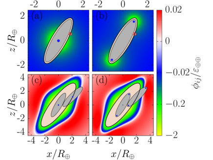
Figure 1: Contour plots of the total interaction potentials $\phi_{ij}=\phi_{\oplus\ominus}$ (Eq. (7)), acting between an ellipsoidal cation ($\oplus$, gray-colored) and a small spherical anion ($\ominus$, red-colored, located at $x/R_{\oplus}\approx 1,z/R_{\oplus}\approx 0.6$), are shown in panels (a) and (b) for $D=0$ and for $D/R_{\oplus}=1.8$, respectively; the orientation $\boldsymbol{\omega}$ of the cation is fixed. The black solid line marks the rim of the small bright excluded volume between the cation and the anion. Beyond the contact distance the pair interaction is purely electrostatic and attractive, with the attraction strongest close to the center for $D=0$ (a) and close to the tips for $D/R_{\oplus}=1.8$ (b), respectively. Panels (c) and (d) provide the cation-cation interaction potentials $\phi_{ij}=\phi_{\oplus\oplus}$ for the same two types of charge distributions of the cations as in (a) and (b). At very short distances the attractive Gay-Berne interaction is dominant, while the electrostatic repulsion is dominant at large distances. In (c) and (d) the attraction is strongest for a parallel orientation of the two cations with a side-to-side positioning. The location of strongest repulsion depends on the position of the charges. The bright excluded volumes in (c) and (d) are much larger than in (a) and (b). Here and in the simulations we have used the parameter values $L_{\oplus}/R_{\oplus}=4$, $\varepsilon_{R_{\oplus}}/\varepsilon_{L_{\oplus}}=3$, $R_{\ominus}/R_{\oplus}=1/4$, $\gamma/(\varepsilon_{\oplus\oplus}R_{\oplus})=0.045$, and $\lambda/R_{\oplus}=5$.

In Fig. 1 the full potentials for the cation-anion and the cation-cation interactions are presented. While panels (a) and (b) show the full cation-anion interaction for $D=0$ and $D/R_{\oplus}=1.8$, respectively, in panels (c) and (d) the cation-cation interaction potential is illustrated for the same types of charge distributions of the cations as in (a) and (b), respectively. For the considered particle sizes, i.e., $L_{\oplus}/R_{\oplus}=4$ and $R_{\ominus}/R_{\oplus}=1/4$, the excluded volume (illustrated by the beige area with a solid black rim) between cations and anions is much smaller compared to the excluded volume between two cations. If $D=0$, the electrostatic interaction is strongest for a side-by-side position of the two considered particles, while for $D/R_{\oplus}=1.8$ it is strongest at the tips. Moreover, the additional electrostatic repulsion among cations leads to a narrowing of the most attractive region (which stems from the attractive Gay-Berne interaction) at close distances for a side-by-side configuration of the cations, if the cation charges are located at the center of the molecule.

II.3 Pair distribution functions

In the course of the simulations the structure of the fluid is analyzed via pair distribution functions. For simulations of bulk systems, the pair distribution functions $g_{ij}(\boldsymbol{r},\boldsymbol{r^{\prime}}):=\varrho_{ij}(\boldsymbol{r}|\boldsymbol{r}^{\prime})/\varrho_{j}$ can be defined as the ratio of the conditional density $\varrho_{ij}(\boldsymbol{r}|\boldsymbol{r}^{\prime})$ of particles of species $i$ at position $\boldsymbol{r}$, provided a particle of species $j$ is located at $\boldsymbol{r^{\prime}}$, and of the constant mean density $\varrho_{j}$ in the simulation box Hansen1986 ; Allen1989 .

As we are mainly interested in observing (smectic) layer structures, we monitor the pair distribution in the direction of the layer normal $\boldsymbol{\hat{n}}$, as well as the particle distribution within the layers, i.e., in directions $\boldsymbol{r}_{\perp}$ lateral to the layer normal. Parallel to the layer normal $\boldsymbol{\hat{n}}$, the statistics along the simulation trajectories invokes all pairs of particles at distances $n:=|(\boldsymbol{r}-\boldsymbol{r^{\prime}})\cdot\boldsymbol{\hat{n}}|$:

$$g_{ij}^{||}(n):=\frac{\varrho_{ij}^{||}(n)}{\varrho_{j}}.$$ (13)

Additionally, for the planes perpendicular to $\boldsymbol{\hat{n}}$ — associated with the vector $\boldsymbol{r}_{\perp}:=\boldsymbol{r}-(\boldsymbol{r}\cdot\boldsymbol{\hat{n}})\boldsymbol{\hat{n}}$ — we monitor the radial distribution of cation pairs via

$$g_{\oplus\oplus}^{(n)}(r_{\perp}):=\frac{\varrho_{\oplus\oplus}^{(n)}(r_{\perp})}{\varrho_{\oplus}},$$ (14)

where $n\in\{0,d\}$ refers to the plane for which $n=0$ and $n=d$, respectively. Thus $g_{\oplus\oplus}^{(0)}(r_{\perp})$ monitors the (cation) pair distribution in the $0$-th plane, i.e., the plane which contains the reference cation at $\boldsymbol{r^{\prime}}$, while $g_{\oplus\oplus}^{(d)}(r_{\perp})$ monitors the distribution of particles in the two neighboring layers, with respect to the cation at $\boldsymbol{r^{\prime}}$.

We add the following remarks concerning the computation of Eqs. (13) and (14):

• The direction of the layer normal $\boldsymbol{\hat{n}}$ is determined by calculating the director DeGennes1974 of each configuration along the simulated trajectories. For the relevant cases, which are analyzed within the scope of the present study, the director and the layer normal point into the same direction, i.e., they are (almost) parallel.

• The evaluation of the conditional densities $\varrho_{ij}^{||}(n)$ and $\varrho_{\oplus\oplus}^{(n)}(r_{\perp})$ requires to count the number of particles which are a distance $n$ and a distance $r_{\perp}$, respectively, apart from the central reference particle. To this end, one considers small but nonzero volumina at $n$ and $r_{\perp}$, which are given by straight slices of width $\Delta n$ and by annuli of width $\Delta r_{\perp}$, respectively. The straight slices for calculating $\varrho_{ij}^{||}(n)$ extend in lateral direction up to the boundaries of the simulation box (see the illustration of such a slice in Fig. 2(a)), while the annuli for calculating $\varrho_{\oplus\oplus}^{(n)}(r_{\perp})$ have an extent in the direction of the layer normal from $\Delta_{||}=1\times R_{\oplus}$ to $\Delta_{||}=2\times R_{\oplus}$.

• While the volume of an annulus is given by $\Delta V^{\perp}=\pi\Delta_{||}\Delta r_{\perp}(\Delta r_{\perp}+2r_{\perp})$, the volumina $\Delta V^{||}$ of the straight slices cannot be calculated straightforwardly, as they are cut off at the boundaries of the simulation box. However, by considering a reference configuration with a homogeneous and isotropic distribution of particles in the simulation box, the volumina of the straight slices can be approximated by $\Delta V^{||}\approx\bar{N}/\varrho^{\text{ref}}$, where $\bar{N}$ denotes the number of particles counted within the considered slices for the isotropic and homogeneous reference configuration of mean density $\varrho^{\text{ref}}$.

III Results

Before presenting our results, we note that the grand canonical Monte Carlo simulations were performed within cubic simulation boxes of volume $V=L^{3}$, where $L:=15R_{\oplus}$. The cation breadth $R_{\oplus}$ is chosen as the unit of length. Standard Metropolis importance sampling has been used Metropolis1953 , invoking the configurational acceptance function $S(\zeta):=-\beta H(\zeta)+\beta\mu N(\zeta)-2\ln((N(\zeta)/2)!)$. Here, $\beta H(\zeta)$ denotes the total (potential) energy of a given configuration $\zeta$ (see Sec. II.1 and Eq. (1)) in units of the thermal energy $k_{B}T=\beta^{-1}$, $\beta\mu$ is the chemical potential, and $N(\zeta)$ is the total number of particles. Since we are considering 1:1-ionic mixtures, there is an equal number of cations and anions, i.e., $N_{\oplus}(\zeta)=N_{\ominus}(\zeta)=N(\zeta)/2$.

Since we are mainly concerned with (smectic) structures formed by the mesogenic cations, the number density is given in terms of the cation packing fraction $\eta:=\frac{\pi}{6}L_{\oplus}R_{\oplus}^{2}\langle N_{\oplus}\rangle/L^{3}$, where $\frac{\pi}{6}L_{\oplus}R_{\oplus}^{2}$ denotes the cation volume and $\langle N_{\oplus}\rangle$ refers to the thermally averaged total number of cations. Temperature is measured in terms of the ratio of the thermal energy $k_{B}T$ and the interaction strength $\varepsilon_{\oplus\oplus}$ of the Gay-Berne potential (Eq. (5)), i.e., $T^{*}:=k_{B}T/\varepsilon_{\oplus\oplus}$.

If not stated otherwise, for the simulations we used the following model parameters: $L_{\oplus}/R_{\oplus}=4$, $\varepsilon_{R_{\oplus}}/\varepsilon_{L_{\oplus}}=3$, $R_{\ominus}/R_{\oplus}=1/4$, $\gamma/(\varepsilon_{\oplus\oplus}R_{\oplus})=0.045$, and $\lambda/R_{\oplus}=5$. Furthermore, for calculating the total energy, all pair interactions (Eq. (1)) have been truncated beyond the range $R_{\text{cut}}/R_{\oplus}=6$.

The phase diagrams displayed in Fig. 4 are obtained by performing simulations for numerous state points $(T^{*},\beta\mu)$, whereby each run is initialized with an isotropic configuration. By performing short additional simulation runs initialized with smectic-A and crystalline configrations, it has been checked for all considered state points that the simulation results do not depend on the initialization. The phase transitions in Fig. 4 are resolved with an accuracy of $\Delta(\beta\mu)=0.1$ in terms of the chemical potential $\beta\mu$. Taking into account the values of $\displaystyle\frac{\partial\eta}{\partial(\beta\mu)}$ obtained from the simulations, this accuracy is sufficient to resolve the white two-phase regions in Fig. 4 with an accuracy of $\displaystyle\Delta\eta\approx\frac{\partial\eta}{\partial(\beta\mu)}\,\Delta(\beta\mu)\leq 0.01$ in terms of the packing fraction $\eta$.

III.1 Dependence of smectic structures on the charge distribution within the cations

III.1.1 Formation of the phase $S_{AW}$

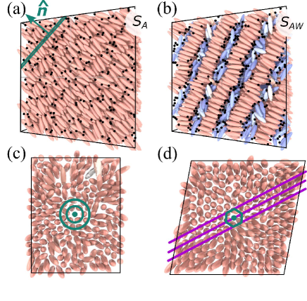
Figure 2: In (a) and (b) we show snapshots of two configurations, belonging to the phases $S_{A}$ and $S_{AW}$, respectively. While for the phase $S_{A}$ a layer spacing of the size of the cation length $L_{\oplus}$ can be observed, and all cations tend to be aligned with the smectic layer normal $\boldsymbol{\hat{n}}$, in (b) the alternating layer structure of the phase $S_{AW}$ is clearly visible. In between the layers of cations, being well-aligned with the layer normal $\boldsymbol{\hat{n}}$ (red-colored ellipsoids), secondary layers are observed, in which the cations are preferentially perpendicular to the layer normal (blue ellipsoids). Due to the alternating layer structure the layer spacing is significantly increased. In panels (a) and (b) the anions are depicted as small black dots, which, however, in order to increase visibility, are three times larger than the actual anions ($R_{\ominus}/R_{\oplus}=1/4$). In (c) and (d) the intra-layer structures of the phases $S_{A}$ and $S_{AW}$, respectively, are shown. While in (c) for the phase $S_{A}$ a fluid-like structure is observed, the snapshot of a main layer of the phase $S_{AW}$ resembles a hexagonal structure (highlighted by the green hexagon and the thick violet lines in panel (d)). This observation is accompanied by a higher cation density within the main layers of the phase $S_{AW}$ as compared with the $S_{A}$ layers. Note, that the green slab in the upper left corner of panel (a) depicts a slice which is used to evaluate the pair distribution functions $g^{||}_{ij}(n)$ in the direction of the layer normal $\boldsymbol{\hat{n}}$ (green arrow). Similarly, in panel (c) the green concentric circles indicate the annulus for calculating the lateral pair distribution function $g^{(n)}_{\oplus\oplus}(r_{\perp})$.

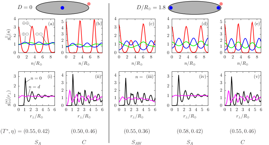
Figure 3: Panels (a) and (b) show the pair distribution functions $g_{ij}^{||}(n)$ in the direction of the smectic layer normal for $D=0$, while panels (c)–(e) correspond to the case $D/R_{\oplus}=1.8$. In the second row, i.e., panels (i)-(v), the corresponding lateral pair distribution functions $g_{\oplus\oplus}^{(n)}(r_{\perp})$ are plotted. (Analogously to the first row, panels (i) and (ii) refer to the case $D=0$ and panels (iii) to (v) to the case $D/R_{\oplus}=1.8$.) In panel (a) a layering of cations with layer spacing $d/R_{\oplus}\approx 3.5\approx L_{\oplus}/R_{\oplus}$ can be inferred from $g_{\oplus\oplus}^{||}(n)$ (red curve). From the corresponding lateral pair distribution function $g_{\oplus\oplus}^{(0)}(r_{\perp})$ (black solid line) in panel (i), a fluid-like structure within the layers can be inferred. Thus, an ordinary smectic-A phase ($S_{A}$) is formed. (The data shown in panels (a) and (i) correspond to the state point $(T^{*}=0.55,\eta\approx 0.42)$, see Fig. 4.) In panels (b) and (ii) a similar layer structure of cations with $d/R_{\oplus}\approx 3.5$ is observed. However, the corresponding state point $(T^{*}=0.5,\eta\approx 0.46)$ is located at a lower temperature $T^{*}$ and at a higher density $\eta$. The strong lateral correlations — even among neighboring layers (see the magenta curve “$n=d$” in panel (ii)) — indicate that this refers to a hexagonal crystal $C$. Both structures for $D=0$ exhibit only a weakly inhomogeneous distribution of anions, i.e., $g_{\oplus\ominus}^{||}(n)$ and $g_{\ominus\ominus}^{||}(n)$ exhibit only minor variations as function of the distance $r_{\perp}$. Panels (c) and (iii) refer to the phase $S_{AW}$ formed for $D/R_{\oplus}=1.8$ at low temperatures and intermediate densities $(T^{*}=0.55,\eta\approx 0.36)$. The alternating layer structure of cations with significantly larger layer spacing $d/R_{\oplus}\approx 6>L_{\oplus}/R_{\oplus}$ is apparent from $g_{\oplus\oplus}^{||}(n)$. Due to the enhanced density within the main cation layers (see the maxima of $g_{\oplus\oplus}^{||}(n)$ at $n=0$ and $n/R_{\oplus}\approx 6$) in lateral directions a hexagonal structure can be observed, unlike the fluid-like lateral structure of the ordinary phase $S_{A}$. However, correlations between cations in neighboring layers are almost absent and thus the phase $S_{AW}$ is a genuine smectic phase and not a crystal. We note that the small variations in $g_{\oplus\oplus}^{(d)}(r_{\perp})$ are artifacts due to the periodic boundary conditions (see the discussion in Sec. III.1 of the main text) and the drop of $g_{\oplus\oplus}^{(d)}(r_{\perp})$ at large distances $r_{\perp}>5$ is another artifact, due to insufficient statistics. Interestingly, for the phase $S_{AW}$ a considerable inhomogeneous distribution of anions (in normal direction) can be observed in panel (c). The anions prefer to be close to the locations of the cation charges in the main layers, e.g., at $n/R_{\oplus}\approx 1.8$, as can be inferred from $g_{\oplus\ominus}^{||}(n)$. Also for $D/R_{\oplus}=1.8$ the ordinary phase $S_{A}$ (at higher temperature $T^{*}=0.58$ and $\eta\approx 0.42$) and the hexagonal crystal $C$ (at $T^{*}=0.55$ and $\eta\approx 0.46$) can be observed (see panels (d) and (iv), respectively (e) and (v)). However, in contrast to the findings for the corresponding phases for $D=0$, for $D/R_{\oplus}=1.8$ the anions exhibit a considerably inhomogeneous spatial distribution. They prefer to be located in between the cation layers, similar to the phase $S_{AW}$.

The present model (see Sec. II) can be understood as an extension of the effective one-species model of ILCs used in previous theoretical studies Kondrat2010 ; Bartsch2015 ; Bartsch2017 , such that the present, extended model accounts for the explicit presence of both ionic species. The present approach allows us to study explicitly the effect of incorporating the valency dependence of the Coulomb interaction on top of the previously studied one-species model. We note, that yet it is necessary to introduce hard-core interactions between the cations and anions, as well as among the anions, in order to avoid divergences in the electrostatic interactions (caused by mutual penetration).

One of the most striking findings within the effective one-species model in Ref. Bartsch2017 is the sensitive dependence of the occurring smectic structures on the location of charges within the ellipsoidal cations. Therefore, we first analyze how the presence of counterions affects this dependence.

We start our analysis at fixed temperature $T^{*}=0.55$ and discuss the structures which are formed at sufficiently high densities, such that the isotropic phase becomes thermodynamically unstable (or at least metastable) with respect to smectic phases. We note that, for the considered parameters, no nematic phase is observed in the density regime between the isotropic and the smectic phase. (For larger values of the cation length-to-breadth ratio $L_{\oplus}/R_{\oplus}$ this might, however, be the case.) Performing Monte Carlo simulations for $D=0$ and $D/R_{\oplus}=1.8$ at $\eta>0.35$, two distinct structures, which are shown in Figs. 2(a) and (b), can be observed. The snapshots show an ordinary smectic-A phase for $D=0$ (a) and the phase $S_{AW}$ for $D/R_{\oplus}=1.8$ (b). While in panel (a) one recognizes a typical smectic layer structure with a layer spacing comparable to the cation length $L_{\oplus}$, in panel (b) alternating layers are observed, in which the cations (illustrated in red) are well-aligned with the layer normal $\boldsymbol{\hat{n}}$, as well as intermediate layers of cations (depicted in blue) which are oriented almost perpendicularly to the layer normal. Interestingly, the intra-layer structure is also different for the two phases. For example for the two layers of the common phase $S_{A}$ and the phase $S_{AW}$ in Figs. 2 (c) and (d), respectively, one observes a (typical) fluid-like structure for the phase $S_{A}$, while a dense and fairly ordered structure is observed for the main layers of the phase $S_{AW}$.

In order to discuss the structure of the two phases in more detail, the pair distribution functions in the direction of the layer normal $\boldsymbol{\hat{n}}$, i.e., $g_{ij}^{||}(n)$, and in lateral directions perpendicular to $\boldsymbol{\hat{n}}$, i.e., $g_{\oplus\oplus}^{(n)}(r_{\perp})$, (compare Eqs. (13) and (14)) are analyzed in Fig. 3. In Figs. 3(a) and (i) the pair distribution functions are shown for the phase $S_{A}$, as depicted in Fig. 2(a), for $D=0$. According to the red curve in Fig. 3(a), the cation-cation correlations, i.e., $g_{\oplus\oplus}^{||}(n)$, clearly show that a layer structure with layer spacing $d/R_{\oplus}\approx 3.5$, comparable to the particle length $L_{\oplus}=4R_{\oplus}$, is formed. Panel (i) shows, for this smectic-A structure, the lateral correlations among the cations, i.e., $g_{\oplus\oplus}^{(n)}(r_{\perp})$. Within the layer in which the reference cation is located (black curve, corresponding to $n=0$), clearly a fluid-like structure with rapidly decaying correlations is observed. For neighboring layers (magenta curve, i.e., $n=d$) one finds no correlations at all. Thus, these findings confirm that the structure shown in Fig. 2(a) is an ordinary smectic-A phase ($S_{A}$).

The phase $S_{AW}$, formed for $D/R_{\oplus}=1.8$, is shown in Figs. 3 (c) and (iii). The cation-cation correlations indicate the alternating layer structure consisting of main layers of high cation density (the peaks of the red curve at $n/R_{\oplus}=0$ and $n/R_{\oplus}\approx 6$) and secondary layers (at $n/R_{\oplus}\approx 3$ and $n/R_{\oplus}\approx 9$). Interestingly, analyzing the lateral structure of the phase $S_{AW}$ in panel (iii), we find a pronounced structure which is distinct from the (fluid-like) pair distribution function obtained for the ordinary phase $S_{A}$. The peak positions yield that this resembles a hexagonal structure, which is also confirmed by the snapshot of a $S_{AW}$ layer, shown in Fig. 2 (d). However, the lateral correlations within the neighboring layer with respect to the reference cation (magenta curve in Fig. 3(iii)) are almost vanishing and therefore the phase $S_{AW}$ is indeed a smectic phase and not a crystal-like structure. Thus, neighboring smectic layers can be sheared without any cost of free energy. We note, that the weak oscillations, which are visible in the magenta curve in Fig. 3(iii), are artifacts of the periodic boundary conditions: If the layer normal is not parallel to one of the main axis of the cubic simulation box, i.e., $\boldsymbol{\hat{n}}\notin\{\boldsymbol{\hat{x}},\boldsymbol{\hat{y}},\boldsymbol{\hat{z}}\}$, the smectic layers are not correctly continued by periodic images of the simulation box. For example, the smectic layer in the lower right corner of Fig. 2(b) is continued to below by the periodic image of the third smectic layer counted from the lower right corner. These artificial correlations (in lateral directions) between neighboring smectic layers occur in principle also for the ordinary phase $S_{A}$. However, due to the short-ranged lateral correlations, they are not visible in Fig. 3(i).

Presumably the different structures of the phases $S_{A}$ and $S_{AW}$ are directly related to the slightly higher density within the main layers of the phase $S_{AW}$ as compared to the layers of the phase $S_{A}$ (see the values of the cation-cation pair distribution function $g^{\|}_{\oplus\oplus}(n)$, i.e., the red curves in Figs. 3(a) and (c), at $n=0$). The higher local cation densities within the $S_{AW}$ main layers are stabilized by the Gay-Berne attraction for parallel oriented cations. Yet, the charges at the tips are indispensable for the formation of the phase $S_{AW}$ as they provide a net repulsion of neighboring smectic layers and therefore make it energetically favorable to maintain a larger distance between the dense main layers separated by the intermediate secondary layers. Given the relatively weak electrostatic interaction as compared to the Gay-Berne attraction (see Fig. 1), already small density differences within the (main) layers of the smectic-A phases decide on the stability of $S_{A}$ or $S_{AW}$. The large layer spacing in combination with the slightly increased density in the main layers and the substantially lower density in the secondary layers rationalizes the intermediate mean density range in which the phase $S_{AW}$ is observed.

For $D=0$, however, the repulsion between cations in neighboring layers is weaker, as compared to the case $D/R_{\oplus}=1.8$ (see the interaction landscape for the two cases in Figs. 1(c) and (d)). Thus, the energetic benefit of a larger layer spacing is insufficient for stabilizing the phase $S_{AW}$ in favor of the phase $S_{A}$ with the layer spacing being comparable to the cation length.

The comparison of the two cases, in which the cation charges are either localized in the center, i.e., $D=0$, or the charges are positioned close to the tips, i.e., $D/R_{\oplus}=1.8$, underscores the importance of the charge distribution within the cations for the formation of the phase $S_{AW}$: In agreement with previous results Bartsch2017 , obtained within the effective one-species model, one can conclude, that, due to the cation charges at the tips, a considerable net repulsion of adjacent (main) layers occurs at small distances (see Fig. 1(d)), which drives the main layers apart to distances larger than the cation length $L_{\oplus}$.

In the case $D/R_{\oplus}=1.8$, apparently the incorporation of explicit anions does not affect the formation of the phase $S_{AW}$. However, as we shall present in the next subsection, the distribution of the anions does sensitively depend on the charge distribution within the cations.

III.1.2 Anion distribution

The different cation charge distributions for $D=0$ and $D/R_{\oplus}=1.8$ not only lead to remarkably different smectic structures, formed by the ellipsoidal cations, but moreover, for the two cases the distribution of anions is also distinct.

Revisiting Fig. 3(a), which depicts the pair distribution functions $g_{ij}^{||}(n)$ along the layer normal for the ordinary smectic-A phase $S_{A}$ for $D=0$, one finds that the anions are rather homogeneously distributed around the layers of cations. (See the green and blue curves which show only minor spatial variations.) The pair distribution function $g_{\oplus\ominus}^{||}(n)$ (blue curve) shows a sparse tendency of the anions to be located in between the cation layers. In contrast, for the phase $S_{AW}$ at the same temperature $T^{*}=0.55$ the anions are strongly pushed out of the main layers formed by the cations. The highest probability to find the anions is close to the location of the charges of the cations in the main layers, i.e., the maxima of $g_{\oplus\ominus}^{||}(n)$ are found at a distance $n/R_{\oplus}\approx D/R_{\oplus}=1.8$ away from the centers of the smectic layers.

A similarly strong inhomogeneous distribution of anions is found for the ordinary phase $S_{A}$ which is formed by cations with $D/R_{\oplus}=1.8$ and at higher temperatures. In Fig. 3(d) the phase $S_{A}$, for $D/R_{\oplus}=1.8$ at the slightly higher temperature $T^{*}=0.58$, is analyzed. While the structure (in normal direction) of the cations (red curve in panel (d)) is very similar to the phase $S_{A}$ formed for $D=0$ (see Figs. 3(a) and (i)), analogously to the case of the phase $S_{AW}$, the anions are preferentially located in between the smectic layers formed by the cations (see the blue curve in panel (d)).

The same findings are obtained for the respective crystal-like phases which are observed in both cases, i.e., for $D=0$ and $D/R_{\oplus}=1.8$, at low temperatures and for large densities (see the detailed discussion of the phase behavior for the two cases in the following Subsec. III.2). Thus we conclude that, for charges at the tips of the cations, not only layer structures of the cations are observed, but also for the anions, although the inhomogeneity in the distribution of the anions is not as pronounced as for the cations. In line with these findings, for $D=0$, i.e., if the charges of the cations are localized in the centers, layering is only observed for the cations. Supposedly, this structural behavior is driven by the interplay of, on the one hand, the electrostatic attraction of the anions towards the cation centers and, on the other hand, with the steric hard-core repulsion, which hinders the anions to penetrate the cation layers.

This striking difference in the anion distributions for the two cases is also relevant for potential applications of ILCs, because some technologies incorporating ILCs like dye-sensitized solar cells (DSSCs) benefit from a higher density of counterions, as they are needed as charge carriers in these applications Yamanaka2005 . Thus, ILCs with charges at the tips, seem to be the best candidates for such applications, whereas cations with $D=0$ seem to be good candidates if a smectic phase of cations in combination with a homogeneous distribution of anions is required.

III.2 Phase behavior

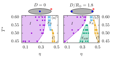
Figure 4: The panels show the phase diagrams for (a) $D=0$ and (b) $D/R_{\oplus}=1.8$. The colored areas represent estimates of the one-phase regions which are obtained by determining thermodynamically stable states (colored dots) generated by the grand canonical MC simulations with isotropic initializations. The white areas are estimates of the two-phase regions, the extensions of which are resolved with an accuracy of $\Delta\eta\leq 0.01$ in terms of the packing fraction $\eta$ (for details see the beginning of Sec. III). It has been checked by means of short additional simulation runs with smectic-A and crystalline initial configurations that the results of the simulations do not depend on the initialization. For $D=0$ (a) at high temperatures $T^{*}\gtrsim 0.52$ a first-order phase transition occurs from the isotropic fluid phase $I$ (violet-colored area) to the ordinary smectic-A phase $S_{A}$ (blue), while at lower temperatures a direct first-order phase transition takes place to the crystalline phase $C$ (yellow) with a hexagonal lattice structure. In contrast, for $D/R_{\oplus}=1.8$ (b) at low temperatures the phase $S_{AW}$ (green) is stable within an intermediate density range, such that, upon increasing $\eta$, first one observes a discontinuous phase transition from the isotropic fluid $I$ to the phase $S_{AW}$, followed at large densities by a first-order phase transition from the phase $S_{AW}$ to the hexagonal crystal $C$.

After having analyzed the differences of the smectic structures associated with the charge distributions $D=0$ and $D/R_{\oplus}=1.8$, we now focus on the phase behavior, i.e., identifying those regions in the $(T^{*},\eta)$ plane, which correspond to the aforementioned distinct structures.

First, we analyze the phase behavior of ILCs consisting of cations with the charges localized in their center, i.e., for $D=0$. Figure 4(a) shows the $T^{*}$-$\eta$ phase diagram for $D=0$. Within the investigated temperature range $T^{*}\in[0.45,0.6]$, the isotropic fluid phase $I$ (violet) is thermodynamically stable up to (cation) packing fractions $\eta\approx 0.25\ {\dots}\ 0.35$. At sufficiently high temperatures $T^{*}\geq 0.52$ a first-order phase transition, indicated by a density gap, is observed to the ordinary smectic-A phase $S_{A}$ (blue). However, at lower temperatures, a direct phase transition to a crystal-like structure $C$ (yellow) occurs. While the phase $S_{A}$ and the crystalline phase $C$ show a rather similar layer spacing $d/R_{\oplus}\approx 3.5$ in normal direction (compare the pair distribution functions $g_{\oplus\oplus}^{||}(n)$ shown in Figs. 3(a) and (b)), their lateral structures are quite distinct. For the phase $C$ a hexagonal ordering (see Fig. 3(ii)) can be observed and, moreover, there are strong correlations between neighboring layers. Indeed, comparing the observed peaks in the distribution functions with an ideal three-dimensional hexagonal lattice, one finds very good agreement concerning the peak positions (in the $0$-th layer, as well as in the neighboring layers). Interestingly, although in general the anions have a tendency to be localized in between the cation layers in the phase $C$, here the distribution of anions is fairly homogeneous (relative to the pronounced peaks in the cation distribution). Thus, while at the considered high densities the cations form a well-marked hexagonal lattice, the anions are still rather motile.

Now we turn to the ILCs with the cation charges at the tips, i.e., $D/R_{\oplus}=1.8$. The corresponding phase diagram is shown in Fig. 4(b). At high temperatures $T^{*}\gtrsim 0.58$ one also finds a first-order phase transition from the isotropic fluid $I$ to the ordinary smectic phase $S_{A}$. Besides the additional inhomogeneous distribution of the anions, which has not been observed for the phase $S_{A}$ for $D=0$ (see Sec. III.1.2), here the smectic-A phase is very similar to the phase $S_{A}$ forming for $D=0$. The layer spacing $d/R_{\oplus}\approx 3.5$ is comparable to the cation length $L_{\oplus}$ and the cations are well-aligned with the layer normal. Furthermore, the lateral correlations (see Fig. 3(iv)) clearly exhibit a fluid-like structure within the smectic layers. If the temperature is lowered to $T^{*}\lesssim 0.55$, a different structure appears. From Figs. 3(c) and (iii) one infers that this distinct structure corresponds to the phase $S_{AW}$ (green). Since the phase $S_{AW}$ emerges in an intermediate density region, for $D/R_{\oplus}=1.8$ the isotropic fluid $I$ is stable only at small densities at low temperatures. An alternating structure of main and secondary layers occurs which leads to a significantly increased layer spacing $d/R_{\oplus}\approx 6.0$. Due to this increased layer spacing, driven by the electrostatic repulsion of neighboring main layers, the bulk densities $\eta$ of the phase $S_{AW}$ are lower than the bulk densities $\eta$ at which the ordinary phase $S_{A}$ is observed. However, by further increasing the number of particles in the system (via raising the chemical potential), at sufficiently high densities the phase $S_{AW}$ becomes metastable with respect to the hexagonal crystal $C$ (see Fig. 4(b) for $T^{*}\lesssim 0.55$ and $\eta\gtrsim 0.4$).

Comparing the present findings with the theoretical predictions of Ref. Bartsch2017 (see Fig. 5 therein), it is remarkable that the DFT results for the effective one-species model, on a qualitative level, predict the stability of the phase $S_{AW}$ in the same thermodynamic region as the present Monte Carlo simulations for the enhanced ILC model, i.e., at low temperatures and at intermediate densities. Furthermore, in both approaches the charge distribution of the (ellipsoidal) cations turns out to be crucial for the formation of the phase $S_{AW}$, i.e., in order to have a stable phase $S_{AW}$ it is indispensable that the charges are close to the tips of the cations.

Finally, it is worth mentioning, that although no stable state points of the phase $C$ have been found at high temperatures, i.e., $T^{*}\gtrsim 0.52$ for $D=0$ and $T^{*}\gtrsim 0.58$ for $D/R_{\oplus}=1.8$, respectively, at sufficiently large densities a crystal-like phase is expected to be the stable configuration, even at high temperatures. Supposedly, with our MC simulations we have been unable to reach the very high density region, which requires a large number of particles in the simulation box and thus slows down the simulations.

IV Summary and conclusions

The objective of the present study is to shed light on the role of counterions in forming smectic structures in ionic liquid crystals (ILCs). In particular, our analysis aims at investigating how the phase behavior and the structural properties of an effective one-species model, which has been employed in previous theoretical studies of ILCs Kondrat2010 ; Bartsch2017 ; Bartsch2019 , are affected by taking the counterions explicitly into account. These previous models represent a simplified description of ILCs, which are composed of anisotropic mesogenic ions (for typical examples, these are cations Binnemans2005 ; Goossens2016 ), which are embedded in a homogeneous screening background consisting of much smaller anions.

The present model, which incorporates both cations and anions on equal footing, can be understood as an improvement of the previous one, because it does not take at the outset any specific distribution of the anions. Thereby it allows one to investigate not only the influence of the anions on the previously observed liquid-crystalline structures Bartsch2017 , but, moreover, the anion distribution by itself can be analyzed, which is of particular interest for potential technological applications of ILCs, e.g., as electrolyte materials in solar cells Yamanaka2005 .

The current coarse-grained model (see Sec. II and Fig. 1) exhibits rigid ellipsoidal cations with two charge sites, symmetrically located at a distance $D$ from the molecular center and spherical anions with one central charge site. All results of this work have been obtained using grand canonical Monte Carlo (MC) simulations.

Depending on the intra-molecular cation charge distribution, distinct smectic structures are observed. They are formed upon increasing the density (expressed in terms of the cation packing fraction $\eta$) such that the isotropic fluid $I$, which is the stable phase at low densities, becomes metastable (and ultimately unstable) with respect to forming smectic layer structures. For $T^{*}=0.55$ a first-order phase transition from the phase $I$ to an ordinary smectic-A phase $S_{A}$ is observed for $\eta>0.35$, if the cations carry a single charge site in their center, i.e., for $D=0$ (see Fig. 2(a)). The designation of the emerged structure as ’smectic-A’ is based on the following observations. The ellipsoidal cations form layers in which they mostly orient parallel to the layer normal $\boldsymbol{\hat{n}}$ and the layer spacing $d\approx 3.5R_{\oplus}$ (Fig. 3(a)) is of the size of the cation length $L_{\oplus}$. Moreover, in the directions which are lateral with respect to $\boldsymbol{\hat{n}}$, i.e., within the smectic layers, a fluid-like structure is observed (see Figs. 2(c) and 3(i)).

In contrast for $D/R_{\oplus}=1.8$, i.e., for cations with charges at their tips, at the same temperature $T^{*}=0.55$ (and at sufficiently high densities, i.e., $\eta\gtrsim 0.3$) a layer structure, which is distinct from the ordinary phase $S_{A}$, is found: Alternating layers of cations are observed, which are mostly parallel to the layer normal $\boldsymbol{\hat{n}}$, and of cations, which are oriented mostly perpendicular to $\boldsymbol{\hat{n}}$ (Fig. 2(b)). This structure can be identified as the wide smectic-A phase $S_{AW}$, which has been found previously Bartsch2017 . In agreement with the previous findings, the (main) layers, in which the cations are well aligned, show a much larger (local) density as compared with the (secondary) layers, in which the cations are mostly perpendicular to $\boldsymbol{\hat{n}}$ (see $g_{\oplus\oplus}^{||}(n)$ in Fig. 3(c)). Moreover, the layer spacing $d\approx 6R_{\oplus}$ of the phase $S_{AW}$ is significantly larger than for the ordinary smectic-A phase $S_{A}$. Due to the high density in the main layers, a lateral hexagonal structure is observed (see Figs. 2(d) and 3(ii)). However, there are no visible correlations among neighboring layers and therefore the phase $S_{AW}$ is a genuine smectic phase and not a crystal.

Interestingly, from comparing the distribution of anions in normal direction $\boldsymbol{\hat{n}}$, we infer that for $D=0$ the anions are rather homogeneously distributed around the cation layers (Figs. 3(a) and (b)), while for $D/R_{\oplus}=1.8$ a pronounced localization of anions in between the cation layers is observed. While for $D=0$ the competing electrostatic attraction and the steric repulsion of cations and anions for small center-to-center distances presumably lead to the fairly homogeneous distribution of anions, for $D/R_{\oplus}=1.8$ the anions are not strongly inhibited by steric repulsion to accumulate at the tips of the cations.

Concerning the phase behavior (see the phase diagrams in Fig. 4) for the currently studied model, we find a remarkable (qualitative) agreement with the previously studied one-species model description of ILC systems. The phase $S_{AW}$ is formed only if the cation charges are positioned at their tips. Furthermore, its stable region is found at lower temperatures, as compared to the ordinary smectic-A phase $S_{A}$, and at intermediate densities, i.e., in particular at lower densities than the ones for the stable phase $S_{A}$ and at higher densities than the ones of the stable isotropic fluid $I$, which is in agreement with the phase behavior predicted by DFT Bartsch2017 . In both cases, i.e., for $D=0$ and $D/R_{\oplus}=1.8$, at very high densities a three-dimensional hexagonal crystal $C$ is formed (see Figs. 3(b) and (ii) as well as Figs. 3(e) and (v), respectively).

These results are not only consistent with the previous findings for the effective one-species description of ILCs, but, moreover, they pinpoint the significance of the (intra-molecular) charge distribution for the phase behavior as well as for the structural properties of ILC systems.

Future studies might focus on the dependence of the thermal behavior and structural properties of ILCs on the anion size and shape, but also on the strength of the Gay-Berne potential as compared to the electrostatic interactions. This, in particular, is a subtle issue, because ILCs typically exhibit an effective charge which is even less than one elementary charge, due to effects like charge delocalization Saielli2017 .

- (1) K. Binnemans, Ionic Liquid Crystals, Chem. Rev. 105, 4148 (2005).
- (2) K. Goossens, K. Lava, C.W. Bielawski, and K. Binnemans, Ionic liquid crystals: versatile materials, Chem. Rev. 116, 4643 (2016).
- (3) S. Kondrat, M. Bier, and L. Harnau, Phase behavior of ionic liquid crystals, J. Chem. Phys. 132, 184901 (2010).
- (4) G. Saielli, T. Margola, and K. Satoh, Tuning Coulombic interactions to stabilize nematic and smectic ionic liquid crystal phases in mixtures of charged soft ellipsoids and spheres, Soft Matter 13, 5204 (2017).
- (5) H. Bartsch, M. Bier, and S. Dietrich, Smectic phases in ionic liquid crystals, J. Phys.: Condens. Matter 29, 464002 (2017).
- (6) H. Bartsch, M. Bier, and S. Dietrich, Interface structures in ionic liquid crystals, Soft Matter 15, 4109 (2019).
- (7) G. Saielli, MD simulation of the mesomorphic behaviour of 1-hexadecyl-3-methylimidazolium nitrate: assessment of the performance of a coarse-grained force field, Soft Matter 8, 10279 (2012).
- (8) B.J. Berne and P. Pechukas, Gaussian Model Potentials for Molecular Interactions, J. Chem. Phys. 56, 4213 (1972).
- (9) J.G. Gay and B.J. Berne, Modification of the overlap potential to mimic a linear site-site potential, J. Chem. Phys. 74, 3316 (1981).
- (10) J.-P. Hansen and I.R. McDonald, Theory of Simple Liquids (Academic, San Diego, 1986).
- (11) P.P. Ewald, Die Berechnung optischer und elektrostatischer Gitterpotentiale, Ann. Physik 369, 253 (1921).
- (12) H. Bartsch, O. Dannenmann, and M. Bier, Thermal and structural properties of ionic fluids, Phys. Rev. E 91, 042146 (2015).
- (13) B. Stenqvist and M. Lund, On short-ranged pair-potentials for long-range electrostatics, Phys. Chem. Chem. Phys. 21, 24787 (2019).
- (14) M.P. Allen and D.J. Tildesley, Computer Simulation of Liquids, (Clarendon, Oxford, 1989).
- (15) P.-G. de Gennes and J. Prost, The Physics of Liquid Crystals (Clarendon, Oxford, 1974).
- (16) N. Metropolis, A.W. Rosenbluth, M.N. Rosenbluth, A.H. Teller, and E. Teller, Equation of State Calculations by Fast Computing Machines, J. Chem. Phys. 21, 1087 (1953).
- (17) N. Yamanaka, R. Kawano, W. Kubo, T. Kitamura, Y. Wada, M. Watanabe, and S. Yanagida, Ionic liquid crystal as a hole transport layer of dye-sensitized solar cells, Chem. Commun. 41, 740 (2005).