DLDL: Dynamic Label Dictionary Learning
via Hypergraph Regularization

Abstract

For classification tasks, dictionary learning based methods have attracted lots of attention in recent years. One popular way to achieve this purpose is to introduce label information to generate a discriminative dictionary to represent samples. However, compared with traditional dictionary learning, this category of methods only achieves significant improvements in supervised learning, and has little positive influence on semi-supervised or unsupervised learning. To tackle this issue, we propose a Dynamic Label Dictionary Learning (DLDL) algorithm to generate the soft label matrix for unlabeled data. Specifically, we employ hypergraph manifold regularization to keep the relations among original data, transformed data, and soft labels consistent. We demonstrate the efficiency of the proposed DLDL approach on two remote sensing datasets.

Index Terms—  Semi-supervised learning, dynamic label dictionary learning, hypergraph manifold, remote sensing image classification

1 Introduction

In recent years, dictionary learning based visual classification tasks have reached or even surpassed human beings’ level. The ultimate goal of dictionary learning is to obtain an overcomplete dictionary to represent samples. Early dictionary learning based methods usually ignore the discriminative information, which is not conducive to represent the connections among different categories. Following, the label information is introduced to solve this problem. Many classical dictionary learning methods, such as LC-KSVD [1], FDDL [2], LEDL [3], incorporated the one-hot label matrix as the constraint term to the objective function. However, these methods only achieve significant improvements in supervised learning (all the training data has labels) tasks. For semi-supervised learning (part of training data has labels) and unsupervised learning (all the training data has no label), the influence of the introduced label information on the dictionary learning framework will be greatly reduced.

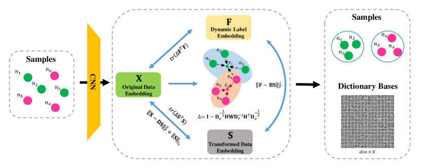
Fig. 1: The DLDL framework. The bule and pink backgrounds denote the hyperedge, we introduce hypergraph Laplacian operator to aggregate vertices. $E_{1}$ and $E_{2}$ represent the aggregated vertex. We construct the connections among $\mathbf{X}$, $\mathbf{S}$ and $\mathbf{F}$ through Equation 8. After that, we obtain dictionary bases to represent samples, which is helpful for classification.

To tackle this issue, we propose the Dynamic Label Dictionary Learning (DLDL) algorithm to dynamically produce soft labels for unlabeled training data, the soft label update with the dictionary learning. Specifically, we introduce hypergraph manifold regularization to construct the connections among the original data, transformed data (after dictionary learning), and soft labels. Graph/hypergraph based manifold structures have been widely applied in different fields, while in our views, most of the works can be split into two categories: $i)$ One is to build the relationship between original data and transformed data, such as HLSC [4], mHDSC [5]. $ii)$ Another one is to construct the connections between original data and predicted labels, including HLPN [6], DHSL [7] et al. Inspired by the two ideas, we try to employ hypergraph manifold regularization to keep the relations among the three ones consistent, which positively influences the classification performance.

In addition, this paper purpose of classifying the remote sensing datasets. Generally, these kinds of datasets have a significant difference among different images. That is to say, there exists a more complicated relationship. However, graph-based methods are powerful ways to represent pair-wise relations for samples, but not suitable in this case. To address this problem, we introduce a hypergraph manifold structure to finish this job. Compared with the graph, hypergraph consists of vertex set and hyperedge set. Each hyperedge includes a flexible number of verices. The structure is capable of modeling the high-order relationship mentioned above. Notably, a hypergraph is the same as a simple graph when the degree of each hyperedge is restricted to $2$. Our proposed DLDL performs well in remote sensing datasets, but it is also applicable to regular datasets. We show the framework of DLDL in Figure 1.

In summary, the main contributions focus on:

• We propose Dynamic Label Dictionary Learning to construct connections among labels, transformed data, and original data by incorporating hypergraph manifold to dictionary learning structure. We make it possible to let the label play an equally important role in supervised, semi-supervised, and unsupervised learning tasks.

• The proposed Dynamic Label block is a model-agnostic method, which is suitable for all subspace learning tasks.

• Experimental results demonstrate that the proposed DLDL significantly improves the classification performance compared with other state-of-the-art dictionary learning methods.

2 Methodology

In this section, we introduce the details of dynamic dictionary learning method, and show the framework in Figure 1.

2.1 Review of Dictionary Learning

Our utilised datasets include training data $\mathbf{X}\in\mathbb{R}^{dim\times N}$ and testing data $\mathbf{Y}\in\mathbb{R}^{dim\times M}$, where ${\mathbf{x}}_{i}$ ($i=1,2,\dots$) is the feature embedding of $i$-th sample and $dim$ denotes the dimension. In dictionary learning, a sparse representation $\mathbf{S}=[{\mathbf{s}}_{1},{\mathbf{s}}_{2},\dots,{\mathbf{s}}_{N}]\in{\mathbb{R}}^{K\times{N}}$ is computed over a dictionary $\mathbf{D}=[{\mathbf{d}}_{1},{\mathbf{d}}_{2},\dots,{\mathbf{d}}_{K}]\in{\mathbb{R}}^{dim\times K}$ by minimizing the reconstruction error, where $K$ is the number of atoms in dictionary. A general dictionary learning algorithm can be formulated as follows:

$$\scriptsize\begin{split}&\mathop{\arg\min}\limits_{{\mathbf{D}},{\mathbf{S}}}f_{1}\left({\mathbf{D}},{\mathbf{S}}\right)=\left\|\mathbf{X}-\mathbf{D}\mathbf{S}\right\|_{F}^{2}+2\alpha\left\|\mathbf{S}\right\|_{\ell_{1}}\\ &{\kern 10.0pt}{\rm{s}}.t.{\kern 4.0pt}\left\|{\mathbf{d}}_{\bullet k}\right\|_{2}^{2}\leq 1,\left({k=1,2,\cdots K}\right)\end{split}$$ (1)

where $\left\|\mathbf{X}-\mathbf{D}\mathbf{S}\right\|_{F}^{2}$ is the reconstruction error, ${\left(\mathbf{d}\right)_{\bullet k}}$ denotes the $k$-th column vector of matrix $\mathbf{D}$. $\left\|\mathbf{S}\right\|_{\ell_{1}}$ represents the sparse constraint for $\mathbf{S}$ (e.g. $\ell_{1}$-norm regularization), and $\alpha$ is a positive scalar constant.

2.2 Dynamic Label Generation via Hypergraph

In this subsection, we first construct the hypergraph, then introduce Laplacian operator to generate dynamic labels.
Hypergraph Construction For any hypergraph based applications, a suitable hypergraph structure is necessary. Different from graph structure, hypergraph can capture high-order relations among samples. We define hypergraph as $\mathcal{G}=(\mathcal{V},\mathcal{E},\mathbf{W})$, where $\mathcal{V}$ denotes the vertex set, each vertex denotes a sample, $\mathcal{E}$ is the hyperedge set, and $\mathbf{W}$ denotes a weight matrix of hyperedge, which is composed of diagonal elements, each element denotes the weight of the corresponding hyperedge. The connection of hyperedges and vertices can be represented by the incidence matrix $\mathbf{H}\in{\mathbb{R}}^{|\mathcal{V}|\times{|\mathcal{E}|}}$. The elements in the incidence matrix are defined as follows:

$$\scriptsize\begin{split}\mathbf{H}=\left\{\begin{array}[]{cc}{\exp\left(-dis\left(v,v_{c}\right)^{2}\right)}&{\text{ if }v\in e}\\ {0}&{\text{ o.w. }}\end{array}\right.\end{split}$$ (2)

where $e$ is one hyperedge among $\mathcal{E}$, $v$ denotes a vertex in $\mathcal{V}$ and $v_{c}$ is the centroid vertex in $e$. $dis$ denotes the operator to compute the distance with knn. Besides, we define two diagonal matrices as $\mathbf{D}_{v}$ (vertex degree matrix) and $\mathbf{D}_{e}$ (hyperedge degree matrix), which are formulated as follows:

$$\scriptsize\begin{split}\delta({e})=\sum_{{v}\in\mathcal{V}}\mathbf{H}({v},{e})\end{split}$$ (3)

$$\scriptsize\begin{split}d({v})=\sum_{{e}\in\mathcal{E}}\mathbf{W}({e})\mathbf{H}({v},{e})\end{split}$$ (4)

Dynamic Label Generation Assume parts of training data have labels, define initial label embedding matrix as $\mathbf{O}\in\mathbb{R}^{C\times N}$, where $C$ denotes the total number of classes. For labeled samples, $\mathbf{O}_{ij}$ is $1$ if the $j$-th sample belongs to the $i$-th class, and it is $0$ otherwise. For unlabeled samples, we set all elements to $0.5$. A suitable label matrix is a good guidance to learn dictionary bases. However, in $\mathbf{O}$, only labeled samples own the correct label embedding, it must interfere with the updating of $\mathbf{D}$ and $\mathbf{S}$. To tackle this problem, we propose a method to generate the dynamic label projection matrix $\mathbf{F}\in\mathbb{R}^{C\times N}$, and embed it into dictionary learning.

It propagates dynamic label information with the joint learning of the incidence matrix $\mathbf{H}$, label projection matrix $\mathbf{F}$, and transformed feature embedding $\mathbf{S}$. We formulate the relationship between $\mathbf{X}$ and $\mathbf{F}$ as follows:

$$\scriptsize\begin{split}&f_{2}\left(\mathbf{F}\right)\\ &=\frac{1}{2}\sum_{c=1}^{C}\sum_{e\in\mathcal{E}}\sum_{u,v\in\mathcal{V}}\frac{\mathbf{W}(e)\mathbf{H}(u,e)\mathbf{H}(v,e)}{\delta(e)}\left(\frac{\mathbf{F}\left(u,c\right)}{\sqrt{d\left(u\right)}}-\frac{\mathbf{F}\left(v,c\right)}{\sqrt{d\left(v\right)}}\right)^{2}\\ &=\text{tr}\left(\left(\mathbf{I}-\mathbf{D}_{v}^{-\frac{1}{2}}\mathbf{H}\mathbf{W}\mathbf{D}_{e}^{-1}\mathbf{H}^{T}\mathbf{D}_{v}^{-\frac{1}{2}}\right)\mathbf{F}^{T}\mathbf{F}\right)\\ &=\text{tr}\left(\mathbf{\Delta}\mathbf{F}^{T}\mathbf{F}\right)\end{split}$$ (5)

where $\mathbf{\Delta}=\mathbf{I}-\mathbf{D}_{v}^{-\frac{1}{2}}\mathbf{H}\mathbf{W}\mathbf{D}_{e}^{-1}\mathbf{H}^{T}\mathbf{D}_{v}^{-\frac{1}{2}}$ denotes the normalized hypergraph Laplacian operator. By this way, we can obtain the smooth $\mathbf{F}$ in label space. Following, we construct connections between $\mathbf{X}$ and $\mathbf{S}$ as:

$$\scriptsize\begin{split}f_{3}\left(\mathbf{S}\right)=\text{tr}\left(\mathbf{\Delta}\mathbf{S}^{T}\mathbf{S}\right)\end{split}$$ (6)

In the end, we introduce the general label constraint term to construct the connections for $\mathbf{F}$ and $\mathbf{S}$, and introduce an empirical loss for $\mathbf{F}$ as follows:

$$\scriptsize\begin{split}f_{4}\left({\mathbf{F},\mathbf{B}},{\mathbf{S}}\right)=\left\|\mathbf{F}-\mathbf{B}\mathbf{S}\right\|_{F}^{2}+\left\|\mathbf{F}-\mathbf{O}\right\|_{F}^{2}\\ \end{split}$$ (7)

where $\mathbf{B}\in\mathbb{R}^{C\times K}$ is the classifier.

2.3 Dynamic Label Dictionary Learning

We summarize the above requirements. The objective function for dynamic label dictionary learning can be written as follows:

$$\scriptsize\begin{split}&\mathop{\arg\min}\limits_{\mathbf{D},\mathbf{S},\mathbf{F},\mathbf{B}}\mathcal{F}(\mathbf{D},\mathbf{S},\mathbf{F},\mathbf{B})\\ &=f_{1}\left({\mathbf{D}},{\mathbf{S}}\right)+f_{2}\left(\mathbf{F}\right)+f_{3}\left(\mathbf{S}\right)+f_{4}\left(\mathbf{F},\mathbf{B},\mathbf{S}\right)\\ &=\left\|\mathbf{X}-\mathbf{D}\mathbf{S}\right\|_{F}^{2}+2\alpha\left\|\mathbf{S}\right\|_{\ell_{1}}+\delta{\kern 2.0pt}\text{tr}\left(\mathbf{\Delta}\mathbf{S}^{T}\mathbf{S}\right)\\ &{\kern 10.0pt}+\beta{\kern 2.0pt}\left\|\mathbf{F}-\mathbf{B}\mathbf{S}\right\|_{F}^{2}+\beta{\kern 2.0pt}\left\|\mathbf{F}-\mathbf{O}\right\|_{F}^{2}+\beta{\kern 2.0pt}\text{tr}\left(\mathbf{\Delta}\mathbf{F}^{T}\mathbf{F}\right)\\ &{\kern 5.0pt}{\rm{s}}.t.\left\|{{{\bf{d}}_{\bullet k}}}\right\|_{2}^{2}\leq 1,{\kern 5.0pt}\left\|{{{\bf{b}}_{\bullet k}}}\right\|_{2}^{2}\leq 1{\kern 4.0pt}\left({k=1,2,\cdots K}\right)\\ \end{split}$$ (8)

where $\beta$, $\delta$ are the balanced parameters for objective function. By this way, we can get the optimal $\mathbf{S}$, $\mathbf{D}$, $\mathbf{B}$ and $\mathbf{F}$ by alternative optimization until the loss dose not descend. Specifically, we update $\mathbf{S}$ with $\mathbf{D}$, $\mathbf{B}$ and $\mathbf{F}$ fixed, the closed form solution of $\mathbf{S}$ is:

$$\scriptsize\begin{split}\mathbf{S}_{kn}={\frac{max\left(\mathcal{J},\alpha\right)+min\left(\mathcal{J},\alpha\right)}{\left(\mathbf{D}^{T}\mathbf{D}+\beta{\kern 2.0pt}\mathbf{B}^{T}\mathbf{B}\right)_{kk}+\delta\left(\mathbf{\Delta}\right)_{nn}}}\end{split}$$ (9)

where

$$\scriptsize\begin{split}\mathcal{J}&=\left(\mathbf{D}^{T}\mathbf{X}+\beta\mathbf{B}^{T}\mathbf{F}\right)_{kn}-\delta\sum_{r=1,r\neq n}^{N}\left(\mathbf{\Delta}\right)_{nr}\mathbf{S}_{kr}\\ &{\kern 10.0pt}-\sum_{l=1,l\neq k}^{K}\left(\mathbf{D}^{T}\mathbf{D}+\beta\mathbf{B}^{T}\mathbf{B}\right)_{kl}\mathbf{S}_{ln}\end{split}$$ (10)

Then we introduce blockwise coordinate descent (BCD) method [8] to directly obtain $\mathbf{D}$ and $\mathbf{B}$ as:

$$\scriptsize\begin{split}\mathbf{D}_{\bullet k}=\frac{\mathbf{X}\left(\mathbf{S}_{k\bullet}\right)^{T}-\mathbf{\tilde{D}}^{k}\mathbf{S}\left(\mathbf{S}_{k\bullet}\right)^{T}}{\|\mathbf{X}\left(\mathbf{S}_{k\bullet}\right)^{T}-\mathbf{\tilde{D}}^{k}\mathbf{S}\left(\mathbf{S}_{k\bullet}\right)^{T}\|_{2}}\end{split}$$ (11)

$$\scriptsize\begin{split}\mathbf{B}_{\bullet k}=\frac{\mathbf{F}\left(\mathbf{S}_{k\bullet}\right)^{T}-\mathbf{\tilde{B}}^{k}\mathbf{S}\left(\mathbf{S}_{k\bullet}\right)^{T}}{\|\mathbf{F}\left(\mathbf{S}_{k\bullet}\right)^{T}-\mathbf{\tilde{B}}^{k}\mathbf{S}\left(\mathbf{S}_{k\bullet}\right)^{T}\|_{2}}\end{split}$$ (12)

where $\mathbf{\tilde{D}}=\left\{\begin{array}[]{cc}{\mathbf{D}_{\bullet p}}&{p\neq{k}}\\ {\mathbf{0}}&{p=k}\end{array}\right.$, $\mathbf{\tilde{B}}=\left\{\begin{array}[]{cc}{\mathbf{B}_{\bullet p}}&{p\neq{k}}\\ {\mathbf{0}}&{p=k}\end{array}\right.$, $\mathbf{0}$ denotes zero matrix. In the end, we update $\mathbf{F}$ with $\mathbf{S}$, $\mathbf{D}$, $\mathbf{B}$ fixed, the closed form solution of $\mathbf{F}$ is:

$$\scriptsize\begin{split}\mathbf{F}=\beta\left(\mathbf{\Delta}+2\beta\mathbf{I}\right)^{-1}\left(\mathbf{B}\mathbf{S}+\mathbf{O}\right)\end{split}$$ (13)

3 Experiment

In this section, in order to fairly evaluate the effectiveness of our DLDL, we compared it with multiple state-of-the-art dictionary learning methods on two remote sensing datasets, include UC Merced Land Use (UCM-LU) [9] and RSSCN7 [10]. We first introduce the experimental setup, and then report the experimental results. At last, we conduct ablation studies to analyze the DLDL method.

3.1 Experimental Setup

For all the datasets, we employ standard Resnet [11] to extract feature embedding with $2,048$ dimensions. Each category has $5$ labeled samples. After that, we fix the dictionary size to $200$ and the nearest number of knn to $10$ for all datasets. The influence of dictionary size is discussed in the following section 3.3. In addition, there are three other parameters ($\alpha$, $\beta$ and $\delta$ ) need to be tuned manually. Here, we give our optimal setups for best performance of DLDL. Specifically, we set $\alpha=2^{-4}$, $\beta=2^{-4}$, $\delta=2^{2}$ for UCM-LU dataset, $\alpha=2^{-4}$, $\beta=2^{-10}$, $\delta=2^{6}$ for RSSCN7 dataset. For some discussions of parameters, please refer to the section 3.3.

3.2 Experimental Results

Table 1: Classification results

Methods$\backslash$Datasets	UCM-LU	RSSCN7
SRC (TPAMI [12], 2009)	80.4$\%$	67.1$\%$
CRC (ICCV [13], 2011)	80.7$\%$	67.7$\%$
NRC (PR [14], 2019)	81.6$\%$	69.7$\%$
SLRC (TPAMI [15], 2018)	81.0$\%$	66.4$\%$
Euler-SRC (AAAI [16], 2018)	80.9$\%$	69.7$\%$
LC-KSVD (TPAMI [1], 2013)	79.4$\%$	68.0$\%$
CSDL (NC [17], 2016)	80.5$\%$	66.7$\%$
LC-PDL (IJCAI [18], 2019)	81.2$\%$	69.7$\%$
FDDL (ICCV [2], 2011)	81.0$\%$	64.0$\%$
LEDL (NC [3], 2020)	80.7$\%$	67.9$\%$
ADDL (TNNLS [19], 2018)	83.2$\%$	72.3$\%$
CDLF (SP [20], 2020)	81.0$\%$	69.6$\%$
HLSC (TPAMI [4], 2012)	81.4$\%$	71.1$\%$
DLDL	85.2$\%$	72.9$\%$

We compare our DLDL with several classical classification methods, include SRC [12], CRC [13], NRC [14], SLRC [15], Euler-SRC [16], LC-KSVD [1], CSDL [17], LC-PDL [18], FDDL [2], LEDL [3], ADDL [19], CDLF [20], HLSC [4]. We show the experimental results in Table 1, and have the following observations.

$i)$ Obviously see that our DLDL outperforms all the other state-of-the-art methods. On the UCM-LU dataset, DLDL achieves the best performance by an improvement of at least $2\%$, and on the RSSCN7 dataset, DLDL is able to exceed other methods at least $0.6\%$.

$ii)$ Compared with traditional label embedded dictionary learning methods, including LC-KSVD, LEDL, CDLF, our proposed dynamic label helps outperform them at least $4.2\%$ on the UCM-LU dataset and $3.3\%$ on the RSSCN7 dataset. For other classical dictionary learning methods, such as CSDL, LC-PDL, FDDL, ADDL, HLSC, our method do not improve much, especially on the RSSCN7 dataset, DLDL only achieves an improvement of $0.6\%$ compared with ADDL. The reason is that all the dictionary learning based methods have their highlights, while our DLDL only introduces the dynamic label to a basic dictionary learning model. In other words, our proposed method is a model-agnostic module, which can be embedded in any dictionary learning based works to promote performance.

3.3 Ablation Study

Our DLDL has achieved outstanding performance. It is necessary to know what the factors affecting the experimental results are. For this purpose, we design two ablation studies to discuss our proposed method further.

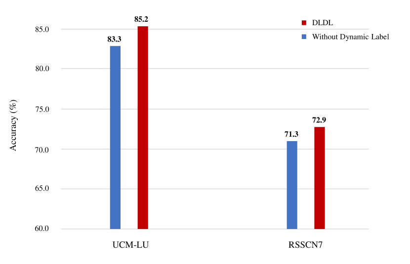
Fig. 2: The influence of dynamic labels.

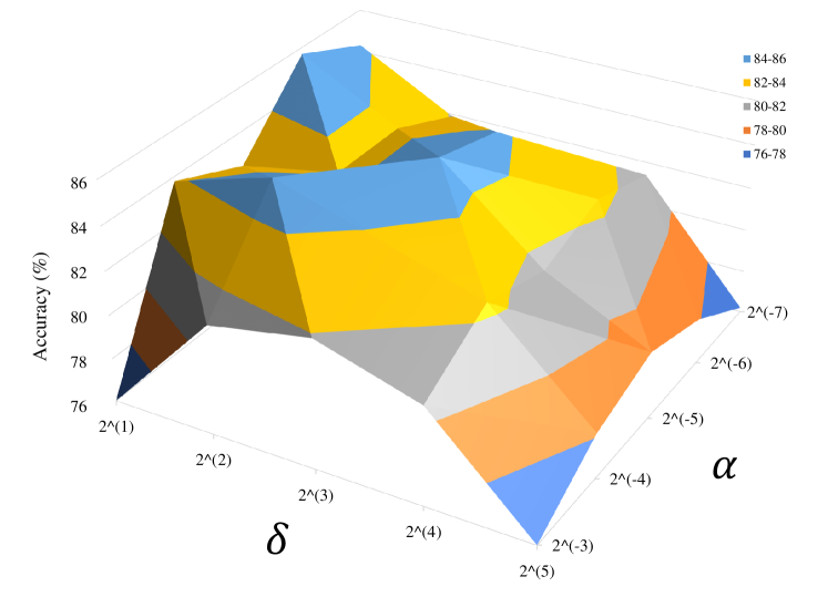
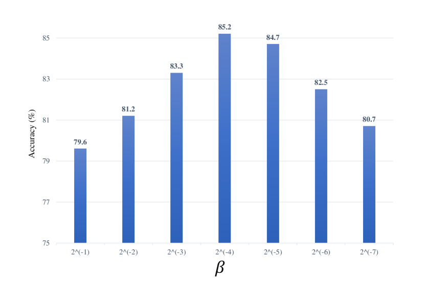
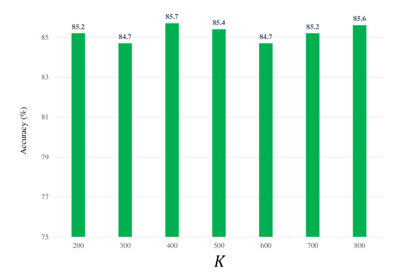
Fig. 3: The influence of parameters

$i)$ To demonstrate the efficiency of the dynamic label, we remove the process for obtaining dynamic labels and replace $\mathbf{F}$ with the fixed one-hot label matrix, where $\mathbf{E}\in\mathbb{R}^{C\times N_{l}}$ denotes the label matrix, $N_{l}$ represents the number of labeled training data. The objective function can be rewritten as:

$$\scriptsize\begin{split}&\mathop{\arg\min}\limits_{\mathbf{D},\mathbf{S},\mathbf{B}}\mathcal{F}(\mathbf{D},\mathbf{S},\mathbf{B})\\ &=\left\|\mathbf{X}-\mathbf{D}\mathbf{S}\right\|_{F}^{2}+2\alpha\left\|\mathbf{S}\right\|_{\ell_{1}}+\beta\left\|\mathbf{E}-\mathbf{B}\mathbf{S_{l}}\right\|_{F}^{2}+\delta{\kern 2.0pt}\text{tr}\left(\mathbf{\Delta}_{l}\mathbf{S}^{T}\mathbf{S}\right)\\ &{\rm{s}}.t.\left\|{{{\mathbf{d}}_{k}}}\right\|_{2}^{2}\leq 1,{\kern 4.0pt}\left\|{{{\mathbf{b}}_{k}}}\right\|_{2}^{2}\leq 1{\kern 4.0pt}\left({k=1,2,\cdots K}\right)\\ \end{split}$$ (14)

where $\mathbf{S}_{l}\in\mathbb{R}^{K\times N_{l}}$ denotes the labeled parts of $\mathbf{S}$. Figure 2 shows the experimental results. From this figure, we find that the dynamic label term has a significant influence on the performance of the two datasets.

$ii)$ In the following experiments, we evaluate the influences of parameters on the UCM-LU dataset. Figure 3 shows the experimental results. In general experience, there are mainly four parameters (e.g. $\alpha$, $\beta$, $\delta$, $K$) affect the experimental results. More specifically, $\beta$ influences the performance independently. Thus we fix $\alpha$, $\delta$ and $K$ to observe the effect. From the figure, we can see that our method is sensitive to $\beta$. For $\alpha$ and $\delta$, they interact with each other. Thus we fix $\beta$ and $K$ to observe the impact of these two parameters simultaneously. We find that our method has strong adaptability to the two parameters, thus we can flexibly choose the pairwise $\alpha$ and $\delta$ to obtain a good performance. Following, we evaluate the influence of dictionary size $K$. In this experiment, we tune the parameters $\alpha$, $\beta$, $\delta$ to obtain the optimal performance for each dictionary size. From the figure, we can conclude that the proposed DLDL approach is not sensitive to the dictionary size. Thus, we would choose a small size to reduce training time.

4 Conclusion

Previous label embedding dictionary learning based methods are not applicable in semi-supervised and unsupervised learning. Thus we propose a Dynamic Label Dictionary Learning (DLDL) algorithm to generate the soft label matrix for unlabeled data. The outstanding performance on two remote sensing datasets has demonstrated the efficiency of the proposed DLDL approach. It would be interesting for future work to expand the dynamic label to other subspace learning tasks.

References

- [1] Zhuolin Jiang, Zhe Lin, and Larry S Davis, “Label consistent k-svd: Learning a discriminative dictionary for recognition,” IEEE Transactions on Pattern Analysis and Machine Intelligence (TPAMI), vol. 35, no. 11, pp. 2651–2664, 2013.
- [2] Meng Yang, Lei Zhang, Xiangchu Feng, and David Zhang, “Fisher discrimination dictionary learning for sparse representation,” in IEEE International Conference on Computer Vision (ICCV). IEEE, 2011, pp. 543–550.
- [3] Shuai Shao, Rui Xu, Weifeng Liu, Bao-Di Liu, and Yan-Jiang Wang, “Label embedded dictionary learning for image classification,” Neurocomputing, vol. 385, pp. 122–131, 2020.
- [4] Shenghua Gao, Ivor Wai-Hung Tsang, and Liang-Tien Chia, “Laplacian sparse coding, hypergraph laplacian sparse coding, and applications,” IEEE Transactions on Pattern Analysis and Machine Intelligence (TPAMI), vol. 35, no. 1, pp. 92–104, 2013.
- [5] Weifeng Liu, Dacheng Tao, Jun Cheng, and Yuanyan Tang, “Multiview hessian discriminative sparse coding for image annotation,” Computer Vision and Image Understanding (CVIU), vol. 118, pp. 50–60, 2014.
- [6] Yubo Zhang, Nan Wang, Yufeng Chen, Changqing Zou, Hai Wan, Xibin Zhao, and Yue Gao, “Hypergraph label propagation network.,” in AAAI Conference on Artificial Intelligence (AAAI), 2020, pp. 6885–6892.
- [7] Zizhao Zhang, Haojie Lin, and Yue Gao, “Dynamic hypergraph structure learning.,” in International Joint Conference on Artificial Intelligence (IJCAI), 2018, pp. 3162–3169.
- [8] Bao-Di Liu, Yu-Xiong Wang, Bin Shen, Yu-Jin Zhang, and Yan-Jiang Wang, “Blockwise coordinate descent schemes for sparse representation,” in IEEE International Conference on Acoustics, Speech and Signal Processing (ICASSP). IEEE, 2014, pp. 5267–5271.
- [9] Yi Yang and Shawn Newsam, “Bag-of-visual-words and spatial extensions for land-use classification,” in International Conference on Advances in Geographic Information Systems (GIS), 2010, pp. 270–279.
- [10] Qin Zou, Lihao Ni, Tong Zhang, and Qian Wang, “Deep learning based feature selection for remote sensing scene classification,” IEEE Geoscience and Remote Sensing Letters (IGRSL), vol. 12, no. 11, pp. 2321–2325, 2015.
- [11] Kaiming He, Xiangyu Zhang, Shaoqing Ren, and Jian Sun, “Deep residual learning for image recognition,” in IEEE Conference on Computer Vision and Pattern Recognition (CVPR), 2016, pp. 770–778.
- [12] John Wright, Allen Y Yang, Arvind Ganesh, S Shankar Sastry, and Yi Ma, “Robust face recognition via sparse representation,” IEEE Transactions on Pattern Analysis and Machine Intelligence (TPAMI), vol. 31, no. 2, pp. 210–227, 2009.
- [13] Lei Zhang, Meng Yang, and Xiangchu Feng, “Sparse representation or collaborative representation: Which helps face recognition?,” in IEEE International Conference on Computer Vision (ICCV). IEEE, 2011, pp. 471–478.
- [14] Jun Xu, Wangpeng An, Lei Zhang, and David Zhang, “Sparse, collaborative, or nonnegative representation: Which helps pattern classification?,” Pattern Recognition (PR), vol. 88, pp. 679–688, 2019.
- [15] Weihong Deng, Jiani Hu, and Jun Guo, “Face recognition via collaborative representation: Its discriminant nature and superposed representation,” IEEE Transactions on Pattern Analysis and Machine Intelligence (TPAMI), vol. 40, no. 10, pp. 2513–2521, 2018.
- [16] Yang Liu, Quanxue Gao, Jungong Han, and Shujian Wang, “Euler sparse representation for image classification,” in AAAI Conference on Artificial Intelligence (AAAI), 2018.
- [17] Bao-Di Liu, Bin Shen, Liangke Gui, Yu-Xiong Wang, Xue Li, Fei Yan, and Yan-Jiang Wang, “Face recognition using class specific dictionary learning for sparse representation and collaborative representation,” Neurocomputing, vol. 204, pp. 198–210, 2016.
- [18] Zhao Zhang, Weiming Jiang, Zheng Zhang, Sheng Li, Guangcan Liu, and Jie Qin, “Scalable block-diagonal locality-constrained projective dictionary learning,” in International Joint Conference on Artificial Intelligence (IJCAI), 2019, pp. 4376–4382.
- [19] Zhao Zhang, Weiming Jiang, Jie Qin, Li Zhang, Fanzhang Li, Min Zhang, and Shuicheng Yan, “Jointly learning structured analysis discriminative dictionary and analysis multiclass classifier,” IEEE Transactions on Neural Networks and Learning Systems (TNNLS), vol. 29, no. 8, pp. 3798–3814, 2018.
- [20] Yan-Jiang Wang, Shuai Shao, Rui Xu, Weifeng Liu, and Bao-Di Liu, “Class specific or shared? a cascaded dictionary learning framework for image classification,” Signal Processing (SP), vol. 176, pp. 107697, 2020.