Learning Implicit Functions for Topology-Varying Dense 3D Shape Correspondence
Abstract
The goal of this paper is to learn dense D shape correspondence for topology-varying objects in an unsupervised manner. Conventional implicit functions estimate the occupancy of a D point given a shape latent code. Instead, our novel implicit function produces a part embedding vector for each D point, which is assumed to be similar to its densely corresponded point in another D shape of the same object category. Furthermore, we implement dense correspondence through an inverse function mapping from the part embedding to a corresponded D point. Both functions are jointly learned with several effective loss functions to realize our assumption, together with the encoder generating the shape latent code. During inference, if a user selects an arbitrary point on the source shape, our algorithm can automatically generate a confidence score indicating whether there is a correspondence on the target shape, as well as the corresponding semantic point if there is one. Such a mechanism inherently benefits man-made objects with different part constitutions. The effectiveness of our approach is demonstrated through unsupervised D semantic correspondence and shape segmentation. Code is available at https://github.com/liuf1990/Implicit_Dense_Correspondence.
1 Introduction
Finding dense correspondence between D shapes is a key algorithmic component in problems such as statistical modeling [4, 56, 5], cross-shape texture mapping [28], and space-time D reconstruction [35]. Dense D shape correspondence can be defined as: given two D shapes belonging to the same object category, one can match an arbitrary point on one shape to its semantically equivalent point on another shape if such a correspondence exists. For instance, given two chairs, the dense correspondence of the middle point on one chair’s arm should be the similar middle point on another chair’s arm, despite different shapes of arms; or alternatively, declare the non-existence of correspondence if another chair has no arm. Although prior dense correspondence methods [37, 30, 15, 18, 42, 29, 48, 31] have proven to be effective on organic shapes, e.g., human bodies and mammals, they become less suitable for generic topology-varying or man-made objects, e.g., chair or vehicles [22].
It remains a challenge to build dense D correspondence for a category with large variations in geometry, structure, and even topology. First of all, the lack of annotations on dense correspondence often leaves unsupervised learning the only option. Second, most prior works make an inadequate assumption [50] that there is a similar topological variability between matched shapes. Man-made objects such as chairs shown in Fig. 1 are particularly challenging to tackle, since they often differ not only by geometric deformations, but also by part constitutions. In these cases, existing correspondence methods for man-made objects either perform fuzzy [27, 47] or part-level [44, 2] correspondences, or predict a constant number of semantic points [19, 8]. As a result, they cannot determine whether the established correspondence is a “missing match” or not. As shown in Fig. 1, for instance, we may find non-convincing correspondences in legs between an office chair and a -legged chair, or even no correspondences in arms for some pairs. Ideally, given a query point on the source shape, a dense correspondence method aims to determine whether there exists a correspondence on the target shape, and the corresponding point if there is. This objective lies at the core of this work.
Shape representation is highly relevant to, and can impact, the approach of dense correspondence. Recently, compared to point cloud [1, 40, 41] or mesh [16, 14, 51], deep implicit functions have shown to be highly effective as D shape representations [38, 33, 32, 43, 9, 10, 3], since it can handle generic shapes of arbitrary topology, which is favorable as a representation for dense correspondence. Often learned as a MLP, conventional implicit functions input the D shape represented by a latent code and a query location in the D space, and estimate its occupancy . In this work, we propose to plant the dense correspondence capability into the implicit function by learning a semantic part embedding. Specifically, we first adopt a branched implicit function [9] to learn a part embedding vector (PEV), , where the max-pooling of gives the . In this way, each branch is tasked to learn a representation for one universal part of the input shape, and PEV represents the occupancy of the point w.r.t. all the branches/semantic parts. By assuming that PEVs between a pair of corresponding points are similar, we then establish dense correspondence via an inverse function mapping the PEV back to the D space. To further satisfy the assumption, we devise an unsupervised learning framework with a joint loss measuring both the occupancy error and shape reconstruction error between and . In addition, a cross-reconstruction loss is proposed to enforce part embedding consistency by mapping within a pair of shapes in the collection. During inference, based on the estimated PEVs, we can produce a confidence score to distinguish whether the established correspondence is valid or not. In summary, contributions of this work include:
We propose a novel paradigm leveraging implicit functions for category-specific unsupervised dense D shape correspondence, which is suitable for objects with diverse variations including varying topology.
We devise several effective loss functions to learn a semantic part embedding, which enables both shape segmentation and dense correspondence. Further, based on the learnt part embedding, our method can estimate a confidence score measuring if the predicted correspondence is valid or not.
Through extensive experiments, we demonstrate the superiority of our method in shape segmentation and D semantic correspondence.

2 Related Work
Dense Shape Correspondence While there are many dense correspondence works for organic shapes [37, 30, 15, 18, 42, 29, 6, 48], due to space, our review focuses on methods designed for man-made objects, including optimization and learning-based methods. For the former, most prior works build correspondences only at a part level [25, 21, 44, 2, 55]. Kim et al. [27] propose a diffusion map to compute point-based “fuzzy correspondence” for every shape pair. This is only effective for a small collection of shapes with limited shape variations. [26] and [20] present a template-based deformation method, which can find point-level correspondences after rigid alignment between the template and target shapes. However, these methods only predict coarse and discrete correspondence, leaving the structural or topological discrepancies between matched parts or part ensembles unresolved.
A series of learning-based methods [53, 19, 49, 34, 54] are proposed to learn local descriptors, and treat correspondence as D semantic landmark estimation. E.g., ShapeUnicode [34] learns a unified embedding for D shapes and demonstrates its ability in correspondence among D shapes. However, these methods require ground-truth pairwise correspondences for training. Recently, Chen et al. [8] present an unsupervised method to estimate D structure points. Unfortunately, it estimates a constant number of sparse structured points. As shapes may have diverse part constitutions, it may not be meaningful to establish the correspondence between all of their points. Groueix et al. [17] also learn a parametric transformation between two surfaces by leveraging cycle-consistency, and apply to the segmentation problem. However, the deformation-based method always deforms all points on one shape to another, even the points from a non-matching part. In contrast, our unsupervisedly learnt model can perform pairwise dense correspondence for any two shapes of a man-made object.
Implicit Shape Representation Due to the advantages of continuous representation and handling complicated topologies, implicit functions have been adopted for learning representations for D shape generation [10, 33, 38, 32], encoding texture [36, 45, 43], and D reconstruction [35]. Meanwhile, some works [24, 23] leverage the implicit representation together with a deformation model for shape registration. However, these methods rely on the deformation model, which might prevent their usage for topology-varying objects. Slavcheva et al. [46] present an approach which implicitly obtains correspondence for organic shapes by predicting the evolution of the signed distance field. However, as they require a Laplacian operator to be invariant, it is limited to small shape variations. Recently, some extensions have been proposed to learn deep structured [13, 12] or segmented implicit functions [9], or separate implicit functions for shape parts [39]. However, instead of at a part level, we extend implicit functions for unsupervised dense shape correspondence.
3 Proposed Method
Let us first formulate the dense D correspondence problem. Given a collection of D shapes of the same object category, one may encode each shape in a latent space . For any point in the source shape , dense D correspondence will find its semantic corresponding point in the target shape if a semantic embedding function (SEF) is able to satisfy
| (1) |
Here the SEF is responsible for mapping a point from its D Euclidean space to the semantic embedding space. When and have sufficiently similar locations in the semantic embedding space, they have similar semantic meaning, or functionality, in their respective shapes. Hence is the corresponding point of . On the other hand, if their distance in the embedding space is too large (), there is not a corresponding point in for . If SEF could be learned for a small , the corresponded point of can be solved via , where is the inverse function of that maps a point from the semantic embedding space back to the D space. Therefore, the dense correspondence amounts to learning the SEF and its inverse function.
Toward this goal, we propose to leverage the topology-free implicit function, a conventional shape representation, to jointly serve as SEF. By assuming that corresponding points are similar in the embedding space, we explicitly implement an inverse function mapping from the embedding space to the D space, so that the learning objectives can be more conveniently defined in the D space rather than the embedding space. Both functions are jointly learned with an occupancy loss for accurate shape representation, and a self-reconstruction loss for the inverse function to recover itself. In addition, we propose a cross-reconstruction loss enforcing two objectives. One is that the two functions can deform source shape points to be sufficiently close to the target shape. The other is that corresponding offset vectors, , are locally smooth within the neighbourhood of .
3.1 Implicit Function and Its Inverse
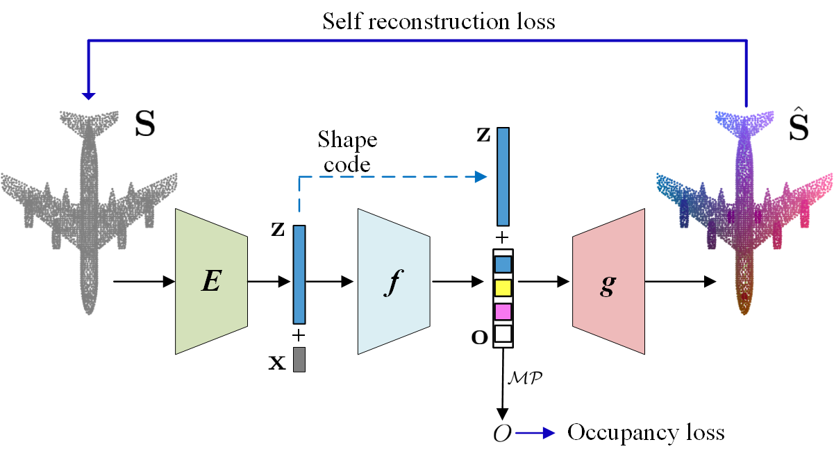
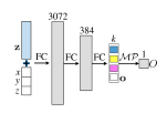
Implicit Function As in [10, 33], a shape is first encoded as a shape code by a PointNet [40]. Given the D coordinate of a query point , the implicit function assigns an occupancy probability between and , where indicates is inside the shape, and outside. This conventional function can not serve as SEF, given its simple D output. Motivated by the unsupervised part segmentation [9], we adopt its branched layer as the final layer of our implicit function, whose output is denoted by in Fig. 2: . A max-pooling operator () leads to the final occupancy by selecting one branch, whose index indicates the unsupervisedly estimated part where belongs to. Conceptually, each element of shall indicate the occupancy value of w.r.t. the respective part. Since appears to represent the occupancy of w.r.t. all semantic parts of the object, the latent space of can be the desirable semantic embedding, and thus we term as the part embedding vector (PEV) of . In our implementation, is composed of fully connected layers each followed by a LeakyReLU, except the final output (Sigmoid).
Inverse Implicit Function Given the objective function in Eqn. 1, one may consider that learning SEF, , would be sufficient for dense correspondence. However, this has two issues. 1) To find correspondence of , we need to compute , i.e., assuming the output of equals and solve for via iterative back-propagation. This can be inefficient during inference. 2) It is easier to define shape-related constraints or losses between and in the D space, than those between and in the embedding space. To this end, we define the inverse implicit function to take PEV and the shape code as inputs, and recover the corresponding D location: . We use a multilayer perception (MLP) network to implement . With , we can efficiently compute via forward passing, without iterative back-propagation.
3.2 Training with Loss Functions
We jointly train our implicit function and inverse function by minimizing three losses: occupancy loss , self-reconstruction loss , and cross-reconstruction loss , i.e.,
| (2) |
where measures how accurately predicts the occupancy of the shapes, enforces is an inverse function of , and strives for part embedding consistency across all shapes in the collection. We first explain how we prepare the training data, then detail our losses.
Training Samples Given a collection of raw D surfaces with consistent upright orientation, we first normalize the raw surfaces by uniformly scaling the object such that the diagonal of its tight bounding box has a constant length and make the surfaces watertight by converting them to voxels. Following the sample scheme of [10], for each shape, we obtain spatial points and their occupancy label , which is for the inside points and otherwise. In addition, we uniformly sample surface points to represent D shapes, resulting in .
Occupancy Loss This is a error between the label and estimated occupancy of all shapes:
| (3) |
Self-Reconstruction Loss We supervise the inverse function by recovering input surface points :
| (4) |
where is the -th vertex of shape .
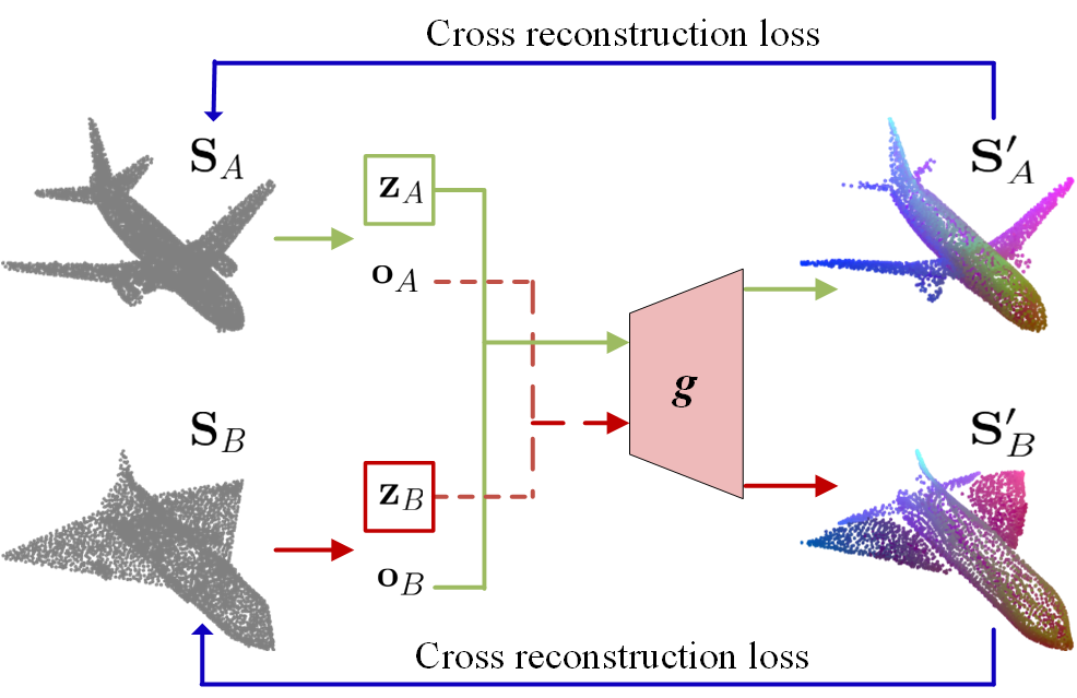
Cross-Reconstruction Loss The cross-reconstruction loss is designed to encourage the resultant PEVs to be similar for densely corresponded points from any two shapes. As in Fig. 2, from a shape collection we first randomly select two shapes and . The implicit function generates PEVs () given () and their respective shape codes () as inputs. Then we swap their PEVs and send the concatenated vectors to the inverse function : , . If the part embedding is point-to-point consistent across all shapes, the inverse function should recover each other, i.e., , . Towards this goal, we exploit several loss functions to minimize the pairwise difference between those shapes:
| (5) |
where is Chamfer distance (CD) loss, Earth Mover distance (EMD) loss, surface normal loss, smooth correspondence loss, and are the weights. The first three terms focus on the shape similarity, while the last one encourages the correspondence offsets to be locally smooth.
Earth mover distance loss is defined as:
| (7) |
where EMD is the minimum of sum of distances between a point in one set and a point in another set over all possible permutations of correspondences [40]: , where is a bijective mapping.
Surface normal loss An appealing property of implicit representation is that the surface normal can be analytically computed using the spatial derivative via back-propagation through the network. Hence, we are able to define the surface normal distance on the point sets.
| (8) |
where is the surface normal of . We measure by the Cosine similarity distance: , where denotes the dot-product.
Smooth correspondence loss encourages that the correspondence offset vectors , of neighboring points are as similar as possible to ensure a smooth deformation:
| (9) |
where , , and are neighborhoods for and respectively.
3.3 Inference
During inference our method can offer both shape segmentation and dense correspondence for D shapes. As each element of PEV learns a compact representation for one common part of the shape collection, the shape segmentation of is the index of the element being max-pooled from its PEV.
As both the implicit function and its inverse are point-based, the number of input points to can be arbitrary during inference. Given two point sets , with shape codes and , generates PEVs and , and outputs cross-reconstructed shape . For any query point , a preliminary correspondence may be found by a nearest neighbour search in : . Knowing the index of in , the same index in refers to the final correspondence . Here, the nearest neighbor search might not be optimal as it limits the solution to the already sampled points in . An alternative is that, once the preliminary correspondence is found, within its neighbourhood, we can search an surface point who is closer to than . As our input shapes are densely sampled, this alternative does not provide notable benefits, and thus we use the first approach. Finally, we compute the correspondence confidence as , where is normalized to the range of , and is the index of in . Since the learned part embedding is discriminative among different parts of a shape, the distance of PEVs is suitable to define the confidence. When is larger than a pre-defined threshold , this correspondence is valid; otherwise has no correspondence.
3.4 Implementation Detail
Our method is trained in three stages: ) PointNet and implicit function are trained on sampled point-value pairs via Eqn. 3. ) , , and inverse function are jointly trained via Eqn. 3 and 4. ) We jointly train , and with . In experiments, we set , , , , , , , . We implement our model in Pytorch and use Adam optimizer at a learning rate of in all stages.
4 Experiments
4.1 3D Semantic Correspondence
Data We evaluate on D semantic point correspondence, a special case of dense correspondence, with two motivations: 1) no database of man-made objects has ground-truth dense correspondence; 2) there is far less prior work in dense correspondence for man-made objects, than the semantic correspondence task, which has strong baselines for comparison. Thus, to evaluate semantic correspondence, we train on ShapeNet [7] and test on BHCP [26] following the setting of [19, 8]. For training, we use a subset of ShapeNet including plane (), bike (), chair () categories to train individual models. For testing, BHCP provides ground-truth semantic points (- per shape) of shapes including plane (), bike (), chair (), helicopter (). We generate all pairs of shapes for testing, e.g., pairs for bike. The helicopter is tested with the plane model as [19, 8] did. As BHCP shapes are with rotations, prior works test on either one or both settings: aligned and unaligned (i.e., vs. arbitrary relative pose of two shapes).
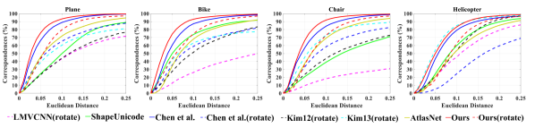
Baseline We compare our work with multiple state-of-the-art (SOTA) baselines. Kim12 [27] and Kim13 [26] are traditional optimization methods that require part label for templates and employ collection-wise co-analysis. LMVCNN [19], ShapeUnicode [34], AtlasNet2 [11] and Chen et al. [8] are all learning based, where [19, 34] require ground-truth correspondence labels for training. Despite [8] only estimates a fixed number of sparse points, [8] and ours are trained without labels. As optimization-based methods and [19] are designed for the unaligned setting, we also train a rotation-invariant version of ours by supervising to predict an additional rotation matrix and applying it to rotate the input point before feeding to .
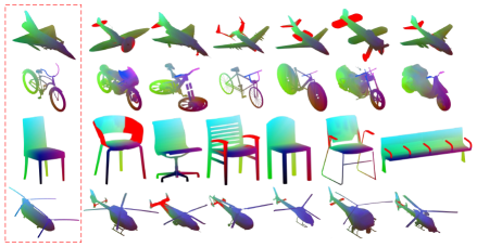
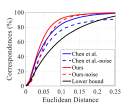
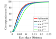
Results The correspondence accuracy is measured by the fraction of correspondences whose error is below a given threshold of Euclidean distances. As in Fig. 3, the solid lines show the results on the aligned data and dotted lines on the unaligned data. We can clearly observe that our method outperforms baselines in plane, bike and chair categories on aligned data. Note that Kim13 [26] has a slightly higher accuracy than ours on the helicopter category, likely due to the fact that [26] tests with the helicopter-specific model, while we test on the unseen helicopter category with a plane-specific model. At the distance threshold of , our method improves on average accuracy in categories over [8]. For unaligned data, our method achieves competitive performance as baselines. While it has the best AUC overall, it is worse at the threshold between . The main reason is the implicit network itself is sensitive to rotation. Note that this comparison shall be viewed in the context that most baselines use extra cues during training or inference, as well as high inference speed of our learning-based approach. Some visual dense correspondence results are shown in Fig. 4. Note the amount of non-existent correspondence is impacted by the threshold as in Fig. 4. A larger discovers more subtle non-existence correspondences. This is expected as the division of semantically corresponded or not can be blurred for some shape parts.
By only finding the closest points on aligned D shapes, we report its semantic correspondence accuracy as the black curve in Fig. 6. Clearly, our accuracy is much higher than this “lower bound", indicating our method doesn’t rely much on the canonical orientation. To further validate on noisy real data, we evaluate on the Chair category with additive noise and compare with Chen et al. [8]. As shown in Fig. 6, the accuracy is slightly worse than testing on clean data. However, our method still outperforms the baseline on noisy data.
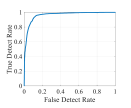
Detecting Non-Existence of Correspondences Our method can build dense correspondences for D shapes with different topologies, and automatically declare the non-existence of correspondence. The experiment in Fig. 3 cannot fully depict this capability of our algorithm as no semantic point was annotated on a non-matching part. Also, there is no benchmark providing the non-existence label between a shape pair. We thus build a dataset with paired shapes from the chair category of ShapeNet part dataset. Within a pair, one has the arm part while the other does not. For the former, we annotate arm points and non-arm points based on provided part labels. As correspondences don’t exist for the arm points, we can utilize this data to measure our detection of non-existence of correspondence. Based on our confidence scores, we report the ROC in Fig. 6. The AUC shows our strong capability in detecting no correspondence.
4.2 Unsupervised Shape Segmentation
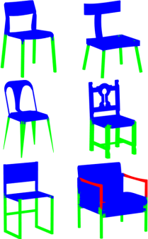
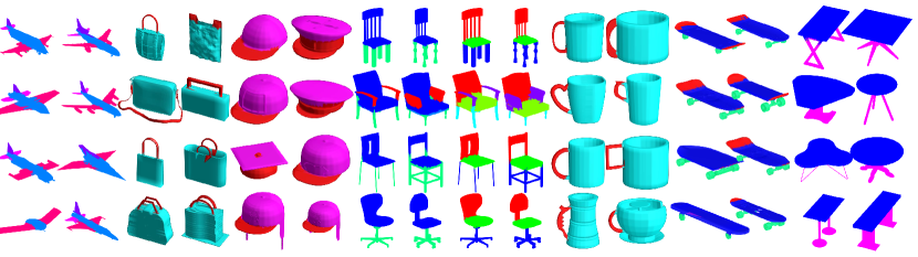
In testing, unlike prior template-based [26] or feature point estimation methods [8], we don’t need to transfer any segmentation labels. Thus, we only compare with the SOTA unsupervised segmentation method BAE-Net [9]. Following the same protocol [9], we train category-specific models and test on the same categories of ShapeNet part dataset [52]: plane (), bag (), cap (), chair (), mug (), skateboard (), table (), and chair* (a joint chair+table set with shapes). Intersection over Union (IoU) between prediction and the ground-truth is a common metric for segmentation. Since unsupervised segmentation is not guaranteed to produce the same part counts exactly as the ground-truth, e.g., combining the seat and back of a chair as one part, we report a modified IoU [9] measuring against both parts and part combinations in the ground-truth. As in Tab. 1, our model achieves a consistently higher segmentation accuracy for all categories than BAE-Net. As BAE-Net is very similar to our model trained in Stage , these results show that our dense correspondence task helps the PEV to better segment the shapes into parts, thus producing a more semantically meaningful embedding. Some visual results of segmentation are shown in Fig. 5.
| Shape (#parts) | plane () | bag () | cap () | chair () | chair* () | mug () | skateboard () | table () | Aver. | |||||||||||||||||
|---|---|---|---|---|---|---|---|---|---|---|---|---|---|---|---|---|---|---|---|---|---|---|---|---|---|---|
|
|
|
|
|
|
|
|
|
||||||||||||||||||
| BAE-Net [9] | ||||||||||||||||||||||||||
| Proposed | 88.0 |
4.3 Ablations and Visualizations
Shape Representation Power of Implicit Function We hope our novel implicit function still serves as a shape representation while achieving dense correspondence. Hence its shape representation power needs to be evaluated. Following the setting of Tab. 1, we first pass a ground-truth point set from the test set to and extract the shape code . By feeding and a grid of points to , we can reconstruct the D shape by Marching Cubes. We evaluate how well the reconstruction matches the ground-truth point set. The average Chamfer distance (CD) between ours and branched implicit function (BAE-Net) on the categories is and (), respectively. The lower CD shows that our novel design of semantic embedding actually improves the shape representation.
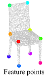
Loss Terms on Correspondence Since the point occupancy loss and self-reconstruction loss are essential, we only ablate each term in the cross-reconstruction loss for the chair category. Correspondence results in Fig. 7 demonstrate that, while all loss terms contribute to the final performance, and are the most crucial ones. forces to resemble . Without , it is possible that may resemble well, but with erroneous correspondences locally.
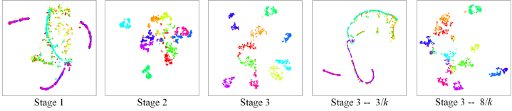
Part Embedding over Training Stages The assumption of learned PEVs being similar for corresponding points motivates our algorithm design. To validate this assumption, we visualize the PEVs of semantic points, defined in Fig. 7, with their ground-truth corresponding points across chairs. The t-SNE visualizes the -dim PEVs in a D plot with one color per semantic point, after each training stage. The model after Stage training resembles BAE-Net. As in Fig. 7, the points corresponding to the same semantic point, i.e., D points of the same color, scatter and overlap with other semantic (colored) points. With the inverse function and self-reconstruction loss in Stage , the part embedding shows more promising grouping of colored points. Finally, the part embedding after Stage has well clustered and more discriminative grouping, which means points corresponding to the same semantic location do have similar PEVs. The improvement trend of part embedding across stages shows the effectiveness of our loss design and training scheme.
One-hot vs. Continuous Embedding Ideally, BAE-Net [9] should output a one-hot vector before , which would benefit unsupervised segmentation the most. In contrast, our PEVs prefer a continuous embedding rather than one-hot. To better understand PEV, we compute the statistics of Cosine Similarity (CS) between the PEVs and their corresponding one-hot vectors: (BAE-Net) vs. (ours). This shows our learnt PEVs are approximately one-hot vectors. Compared to BAE-Net, our smaller CS and larger variance are likely due to the limited network capability, as well as our encouragement to learn a continuous embedding benefiting correspondence.
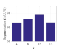
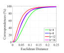
Dimensionality of PEV Fig. 6 and 6 show the shape segmentation and semantic correspondence results over the dimensionality of PEV. Our algorithm performs the best in both when . Despite unsupervisedly segmenting chairs into parts, the extra dimensions of PEV benefit the finer-grained task of correspondence (Fig. 7), which in turns help segmentation.
Computation Time Our training on one category ( samples) takes hours to converge with a GTXTi GPU, where , , and hours are spent at Stage , , respectively. In inference, the average runtime to pair two shapes () is second including runtimes of , , networks, neighbour search and confidence calculation.
5 Conclusion
In this work, we propose a novel framework including an implicit function and its inverse for dense D shape correspondences of topology-varying objects. Based on the learnt semantic part embedding via our implicit function, dense correspondence is established via the inverse function mapping from the part embedding to the corresponding D point. In addition, our algorithm can automatically calculate a confidence score measuring the probability of correspondence, which is desirable for man-made objects with large topological variations. The comprehensive experimental results show the superiority of the proposed method in unsupervised shape correspondence and segmentation.
Broader Impact
Product design (e.g., furniture ) is labor extensive and requires expertise in computer graphics. With the increasing number and diversity of D CAD models in online repositories, there is a growing need for leverage them to facilitate future product development due to their similarities in function and shape. Towards this goal, our proposed method provide a novel unsupervised paradigm to establish dense correspondence for topology-varying objects, which is a prerequisite for shape analysis and synthesis. Furthermore, as our approach is designed for generic objects, its application space can be extremely wide.
Acknowledgement
We acknowledge Vladimir G. Kim and Nenglun Chen for sharing data and results.
Supplementary
In this supplementary material, we provide:
Implementation details, including network structures and training details.
Additional experimental results, including expressiveness of the inverse implicit function and visualization of the correspondence confidence score.
A Implementation Details
A.1 Network Structures
PointNet Encoder .
Implicit Function .
The implicit function network follows the work of [9] (unsupervised case). The implicit function takes the shape code and a spatial point as inputs and predicts the part embedding vector (PEV) . As shown in Fig. 8(b), it is composed of fully connected (FC) layers each of which is applied with , except the final output is applied a activation.
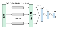
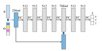
Inverse Implicit Function .
The inverse implicit function is also implemented as an MLP, which is composed of FC layers each of which is applied with , except the final output is applied a activation. As shown in Fig 8(c), the inverse implicit function network inputs the PEVs and shape latent code, and recover the corresponding D points.
A.2 Training Details
Sampling Point-Value Pairs.
The training of implicit function network needs point-value pairs. Following the sampling strategy of [10], we obtain the paired data offline. are the spatial point and the corresponding occupancy label. We sample points from the voxel models in different resolutions: (), () and () in order to train the implicit function progressively.
Training Process
We summarize the training process in Tab. 2. In Stage , we adopt a progressive training technique [10] to train our implicit function on gradually increasing resolution data (), which stabilizes and significantly speeds up the training process.
| Network | Loss | |
|---|---|---|
| Stage | , | |
| Stage | , , | and |
| Stage | , , |
B Additional Experimental Results
A supplementary video is provided to visualize additional results, explained as follows.
B.1 Expressiveness of Inverse Implicit Function
Given our inverse implicit function, we are able to cross-reconstruct each other between two paired shapes by swapping their part embedding vectors. Further, we can interpolate shapes both in shape latent space and D space and maintain the point-level correspondence consistently.
Cross-Reconstruction Performance.
We first show the cross-reconstruction performances in the supplementary video. From a shape collection, we can randomly select two shapes and . Their shape codes and can be predicted by the PointNet encoder. With their respectively generated PEVs and , we can swap their PEVs and send the concatenated vectors to the inverse function and obtain , . As shown in the video, the cross reconstructions closely resemble each other, even with different part constitutions. Here, we also provide the cross-reconstruction performance of two additional object categories: car and table.
Interpolation in Latent Space.
An alternative way to explore the correspondence ability of the inverse implicit function, is to evaluate the interpolation capability of the inverse implicit function. In this experiment, we first interpolate shapes in the latent space (), and send the concatenated vectors ( and ) to the inverse function. As observed in the video, our inverse implicit function generalizes well the different shape deformations. Moreover, the correspondences are point-to-point consistent across all the deformations. It also demonstrates that the learned part embedding is discriminative among different parts of shape and point-wise consistent among different shapes.
Latent Interpolation Comparison.
We compare the latent interpolate capability with conventional implicit function. For the conventional implicit function, we sample a grid of points and pass them to the implicit function to obtain its value. With the threshold of , we obtain the surface points. As can be observed in the video, the interpolation performance of our inverse implicit function is better than conventional implicit function in shape generation and deformation. Furthermore, our interpolations are point-to-point correspondence across all the deformations.
Interpolation in 3D Space.
We also show the interpolation capability of the corresponding points in the D space in the video. Given the estimated dense correspondence, we can compute the correspondence offset vectors for all corresponding pairs of points. Assuming we interpolate the correspondence in video frames, for each frame we move all points of by the amount of and show the moved points. It can be observed that our deformed shape is meaningful and a semantic blending of two shapes. In addition, the correspondence offsets are locally smooth in the D space.
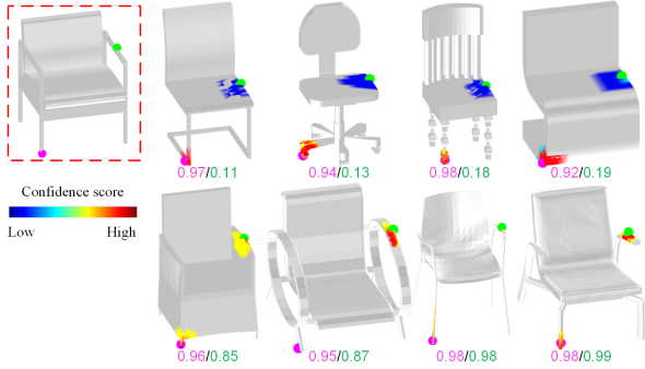
B.2 Visualization of the Correspondence Confidence Score
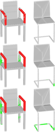
To further visualize the correspondence confidence score, we provide the confidence score maps for some examples in Figure of the paper. As shown in the video, the confidence score can show the probability around corresponded points between the target shape (red box) and its pair-wise source shapes. For example, for the source shapes with arms, we can clearly see the confidence scores of the arm part is significantly lower than other parts.
References
- [1] Panos Achlioptas, Olga Diamanti, Ioannis Mitliagkas, and Leonidas Guibas. Learning representations and generative models for 3D point clouds. In ICML, 2018.
- [2] Ibraheem Alhashim, Kai Xu, Yixin Zhuang, Junjie Cao, Patricio Simari, and Hao Zhang. Deformation-driven topology-varying 3D shape correspondence. TOG, 2015.
- [3] Matan Atzmon, Niv Haim, Lior Yariv, Ofer Israelov, Haggai Maron, and Yaron Lipman. Controlling neural level sets. In NeurIPS, 2019.
- [4] Volker Blanz and Thomas Vetter. Face recognition based on fitting a 3D morphable model. TPAMI, 2003.
- [5] Federica Bogo, Javier Romero, Matthew Loper, and Michael J Black. FAUST: Dataset and evaluation for 3D mesh registration. In CVPR, 2014.
- [6] Davide Boscaini, Jonathan Masci, Emanuele Rodolà, and Michael Bronstein. Learning shape correspondence with anisotropic convolutional neural networks. In NeurIPS, 2016.
- [7] Angel X. Chang, Thomas Funkhouser, Leonidas Guibas, Pat Hanrahan, Qixing Huang, Zimo Li, Silvio Savarese, Manolis Savva, Shuran Song, Hao Su, Jianxiong Xiao, Li Yi, and Fisher Yu. ShapeNet: An information-rich 3D model repository. arXiv preprint arXiv:1512.03012, 2015.
- [8] Nenglun Chen, Lingjie Liu, Zhiming Cui, Runnan Chen, Duygu Ceylan, Changhe Tu, and Wenping Wang. Unsupervised learning of intrinsic structural representation points. In CVPR, 2020.
- [9] Zhiqin Chen, Kangxue Yin, Matthew Fisher, Siddhartha Chaudhuri, and Hao Zhang. BAE-NET: branched autoencoder for shape co-segmentation. In ICCV, 2019.
- [10] Zhiqin Chen and Hao Zhang. Learning implicit fields for generative shape modeling. In CVPR, 2019.
- [11] Theo Deprelle, Thibault Groueix, Matthew Fisher, Vladimir Kim, Bryan Russell, and Mathieu Aubry. Learning elementary structures for 3D shape generation and matching. In NeurIPS, 2019.
- [12] Kyle Genova, Forrester Cole, Avneesh Sud, Aaron Sarna, and Thomas Funkhouser. Local deep implicit functions for 3D shape. In CVPR, 2020.
- [13] Kyle Genova, Forrester Cole, Daniel Vlasic, Aaron Sarna, William T Freeman, and Thomas Funkhouser. Learning shape templates with structured implicit functions. In ICCV, 2019.
- [14] Justin Johnson Georgia Gkioxari, Jitendra Malik. Mesh R-CNN. In ICCV, 2019.
- [15] Thibault Groueix, Matthew Fisher, Vladimir G Kim, Bryan C Russell, and Mathieu Aubry. 3D-CODED: 3D correspondences by deep deformation. In ECCV, 2018.
- [16] Thibault Groueix, Matthew Fisher, Vladimir G Kim, Bryan C Russell, and Mathieu Aubry. Atlasnet: A papier-mâché approach to learning 3D surface generation. In CVPR, 2018.
- [17] Thibault Groueix, Matthew Fisher, Vladimir G Kim, Bryan C Russell, and Mathieu Aubry. Unsupervised cycle-consistent deformation for shape matching. In Computer Graphics Forum, 2019.
- [18] Oshri Halimi, Or Litany, Emanuele Rodola, Alex M Bronstein, and Ron Kimmel. Unsupervised learning of dense shape correspondence. In CVPR, 2019.
- [19] Haibin Huang, Evangelos Kalogerakis, Siddhartha Chaudhuri, Duygu Ceylan, Vladimir G Kim, and Ersin Yumer. Learning local shape descriptors from part correspondences with multiview convolutional networks. TOG, 2017.
- [20] Haibin Huang, Evangelos Kalogerakis, and Benjamin Marlin. Analysis and synthesis of 3D shape families via deep-learned generative models of surfaces. In Computer Graphics Forum, 2015.
- [21] Qixing Huang, Vladlen Koltun, and Leonidas Guibas. Joint shape segmentation with linear programming. In SIGGRAPH Asia, 2011.
- [22] Qixing Huang, Fan Wang, and Leonidas Guibas. Functional map networks for analyzing and exploring large shape collections. TOG, 2014.
- [23] Xiaolei Huang, Nikos Paragios, and Dimitris N Metaxas. Shape registration in implicit spaces using information theory and free form deformations. TPAMI, 2006.
- [24] Xiaolei Huang, Song Zhang, Yang Wang, Dimitris Metaxas, and Dimitris Samaras. A hierarchical framework for high resolution facial expression tracking. In CVPRW, 2004.
- [25] Evangelos Kalogerakis, Aaron Hertzmann, and Karan Singh. Learning 3D mesh segmentation and labeling. In SIGGRAPH, 2010.
- [26] Vladimir G Kim, Wilmot Li, Niloy J Mitra, Siddhartha Chaudhuri, Stephen DiVerdi, and Thomas Funkhouser. Learning part-based templates from large collections of 3D shapes. TOG, 2013.
- [27] Vladimir G Kim, Wilmot Li, Niloy J Mitra, Stephen DiVerdi, and Thomas Funkhouser. Exploring collections of 3D models using fuzzy correspondences. TOG, 2012.
- [28] Vladislav Kraevoy, Alla Sheffer, and Craig Gotsman. Matchmaker: constructing constrained texture maps. TOG, 2003.
- [29] Sing Chun Lee and Misha Kazhdan. Dense point-to-point correspondences between genus-zero shapes. In Computer Graphics Forum, 2019.
- [30] Or Litany, Tal Remez, Emanuele Rodolà, Alex Bronstein, and Michael Bronstein. Deep functional maps: Structured prediction for dense shape correspondence. In ICCV, 2017.
- [31] Feng Liu, Luan Tran, and Xiaoming Liu. 3D face modeling from diverse raw scan data. In ICCV, 2019.
- [32] Shichen Liu, Shunsuke Saito, Weikai Chen, and Hao Li. Learning to infer implicit surfaces without 3D supervision. In NeurIPS, 2019.
- [33] Lars Mescheder, Michael Oechsle, Michael Niemeyer, Sebastian Nowozin, and Andreas Geiger. Occupancy networks: Learning 3D reconstruction in function space. In CVPR, 2019.
- [34] Sanjeev Muralikrishnan, Vladimir G Kim, Matthew Fisher, and Siddhartha Chaudhuri. Shape unicode: A unified shape representation. In CVPR, 2019.
- [35] Michael Niemeyer, Lars Mescheder, Michael Oechsle, and Andreas Geiger. Occupancy flow: 4D reconstruction by learning particle dynamics. In ICCV, 2019.
- [36] Michael Oechsle, Lars Mescheder, Michael Niemeyer, Thilo Strauss, and Andreas Geiger. Texture fields: Learning texture representations in function space. In ICCV, 2019.
- [37] Maks Ovsjanikov, Mirela Ben-Chen, Justin Solomon, Adrian Butscher, and Leonidas Guibas. Functional maps: a flexible representation of maps between shapes. TOG, 2012.
- [38] Jeong Joon Park, Peter Florence, Julian Straub, Richard Newcombe, and Steven Lovegrove. DeepSDF: Learning continuous signed distance functions for shape representation. In CVPR, 2019.
- [39] Despoina Paschalidou, Luc van Gool, and Andreas Geiger. Learning unsupervised hierarchical part decomposition of 3D objects from a single rgb image. In CVPR, 2020.
- [40] Charles R Qi, Hao Su, Kaichun Mo, and Leonidas J Guibas. Pointnet: Deep learning on point sets for 3D classification and segmentation. In CVPR, 2017.
- [41] Charles Ruizhongtai Qi, Li Yi, Hao Su, and Leonidas J Guibas. Pointnet++: Deep hierarchical feature learning on point sets in a metric space. In NeurIPS, 2017.
- [42] Jean-Michel Roufosse, Abhishek Sharma, and Maks Ovsjanikov. Unsupervised deep learning for structured shape matching. In ICCV, 2019.
- [43] Shunsuke Saito, Zeng Huang, Ryota Natsume, Shigeo Morishima, Angjoo Kanazawa, and Hao Li. PIFu: Pixel-aligned implicit function for high-resolution clothed human digitization. In ICCV, 2019.
- [44] Oana Sidi, Oliver van Kaick, Yanir Kleiman, Hao Zhang, and Daniel Cohen-Or. Unsupervised co-segmentation of a set of shapes via descriptor-space spectral clustering. In SIGGRAPH Asia, 2011.
- [45] Vincent Sitzmann, Michael Zollhöfer, and Gordon Wetzstein. Scene representation networks: Continuous 3D-structure-aware neural scene representations. In NeurIPS, 2019.
- [46] Miroslava Slavcheva, Maximilian Baust, and Slobodan Ilic. Towards implicit correspondence in signed distance field evolution. In ICCV, 2017.
- [47] Justin Solomon, Andy Nguyen, Adrian Butscher, Mirela Ben-Chen, and Leonidas Guibas. Soft maps between surfaces. In Computer Graphics Forum, 2012.
- [48] Florian Steinke, Volker Blanz, and Bernhard Schölkopf. Learning dense 3D correspondence. In NeurIPS, 2007.
- [49] Minhyuk Sung, Hao Su, Ronald Yu, and Leonidas J Guibas. Deep functional dictionaries: Learning consistent semantic structures on 3D models from functions. In NeurIPS, 2018.
- [50] Oliver Van Kaick, Hao Zhang, Ghassan Hamarneh, and Daniel Cohen-Or. A survey on shape correspondence. In Computer Graphics Forum, 2011.
- [51] Nanyang Wang, Yinda Zhang, Zhuwen Li, Yanwei Fu, Wei Liu, and Yu-Gang Jiang. Pixel2mesh: Generating 3D mesh models from single RGB images. In ECCV, 2018.
- [52] Li Yi, Vladimir G Kim, Duygu Ceylan, I-Chao Shen, Mengyan Yan, Hao Su, Cewu Lu, Qixing Huang, Alla Sheffer, and Leonidas Guibas. A scalable active framework for region annotation in 3D shape collections. TOG, 2016.
- [53] Li Yi, Hao Su, Xingwen Guo, and Leonidas J Guibas. SyncspecCNN: Synchronized spectral CNN for 3D shape segmentation. In CVPR, 2017.
- [54] Yang You, Yujing Lou, Chengkun Li, Zhoujun Cheng, Liangwei Li, Lizhuang Ma, Cewu Lu, and Weiming Wang. Keypointnet: A large-scale 3D keypoint dataset aggregated from numerous human annotations. In CVPR, 2020.
- [55] Chenyang Zhu, Renjiao Yi, Wallace Lira, Ibraheem Alhashim, Kai Xu, and Hao Zhang. Deformation-driven shape correspondence via shape recognition. TOG, 2017.
- [56] Silvia Zuffi, Angjoo Kanazawa, David W Jacobs, and Michael J Black. 3D menagerie: Modeling the 3D shape and pose of animals. In CVPR, 2017.