A Modular Framework for Distributed Model Predictive Control of Nonlinear Continuous-Time Systems (GRAMPC-D)

Abstract

The modular open-source framework GRAMPC-D for model predictive control of distributed systems is presented in this paper. The modular concept allows to solve optimal control problems (OCP) in a centralized and distributed fashion using the same problem description. It is tailored to computational efficiency with the focus on embedded hardware. The distributed solution is based on the Alternating Direction Method of Multipliers ($\mathrm{ADMM}$) and uses the concept of neighbor approximation to enhance convergence speed. The presented framework can be accessed through C++ and Python and also supports plug-and-play and data exchange between agents over a network.

1 Introduction

Model predictive control (MPC) is a modern control concept that attained increasing attention during the last decades bib:mayne2000 ; bib:allgower2012 as it is capable to handle nonlinear systems while considering constraints on both states and controls. It is based on solving an optimal control problem (OCP) on a finite horizon and applying the first part of the control trajectory to the actual plant, corresponding to the sampling time $\Delta_{t}$ of the controller. At the next sampling instant, the horizon is shifted and the OCP is solved again. This iterative scheme is executed repetitively to stabilize the plant on an infinite horizon.

A main difficulty is the computational complexity of solving the OCP in real-time, which in turn requires an efficient implementation of suitable MPC algorithms. In the recent past, several toolboxes were published that provide adequate software frameworks such as ACADO bib:houska2011 and ACADOS bib:verschueren2019 , VIATOC bib:kalmari2015 or GRAMPC  bib:kapernick2014 ; bib:englert2019 . In case of distributed systems with a high number of controls and states, the classic centralized approach is not capable of solving the overall OCP in real-time anymore. Hence, algorithms for distributed model predictive control (DMPC) bib:camponogara2002 ; bib:maestre2014 have been in the focus over the last years. Their basic idea is to decouple the centralized OCP and to split it into multiple local OCPs that can be solved in parallel. The expectation is to compensate the higher computational complexity due to the decoupled formulation as well as the increased communication effort by the parallel structure. There are multiple approaches to distributed algorithms for optimal control problems, such as sensitivity-based algorithms bib:scheu2011 , the augmented Lagrangian based alternating direction inexact Newton method ($\mathrm{ALADIN}$) bib:houska2016 ; bib:houska2018 or the alternating direction method of multipliers ($\mathrm{ADMM}$) bib:boyd2011 that is also used in the presented framework.

The difficulty of an efficient implementation is drastically higher in case of DMPC than for classic MPC algorithms, as a potentially high number of subsystems, so-called agents, have to be managed. Several toolboxes for DMPC have been published as well. Linear discrete-time systems are considered in the DMPC-Toolbox bib:gafvert2014 that is implemented in Matlab. The PnPMPC-TOOLBOX bib:pnpmpctoolbox2013 focuses on the plug-and-play functionality and provides an implementation in Matlab that considers continuous-time and discrete-time linear systems. Several algorithms are implemented in the Python-Toolbox DISROPT bib:farina2019 regarding distributed optimization problems. ALADIN-$\alpha$ bib:engelmann2020 is the most recent published toolbox that provides a Matlab implementation of the ALADIN algorithm. However, there is a lack of a DMPC framework that provides an implementation tailored to embedded hardware with the focus on real-time capable distributed model predictive control. Many real-world problems such as smart grids or cooperative robot applications are only equipped with weak hardware on the subsystem level that is not able to handle complex computation tasks in an appropriate time. Hence, for realizing distributed controllers on actual plants, an implementation optimized on execution time is required to enable real-time control. Furthermore, providing the possibility of communication between agents over a network is essential for a DMPC framework designed to control actual plants. The restriction to neighbor-to-neighbor-communication decouples the agents communication effort from the overall system size by bounding it to the cardinality of its neighborhood. The focus on real-world plants requires the system class to cover nonlinear dynamics including couplings between the agents in both dynamics and constraints.

The presented framework, in the following GRAMPC-D, provides an open-source C++ implementation that is capable of solving optimal control problems in a distributed manner with a per-agent computation-time in the millisecond range. The underlying minimization problems are solved with the $\mathrm{MPC}$ toolbox GRAMPC that is suitable for embedded hardware implementations. However, other toolboxes for solving the local minimization problem can be used as well. To enable actual distributed optimization, a socket-based TCP communication is provided to allow agents to exchange data over a network. Furthermore, a Python interface is provided in addition to the C++-interface using the software module Pybind11 bib:pybind11 . The Python interface combines both the functionality of Python and the performance of C++ as it only wraps the C++ interface while the actual code executing the $\mathrm{DMPC}$ algorithm is still running in C++. Furthermore, it allows for fast and efficient prototyping when developing a controller for a distributed system as both a centralized as well as a distributed controller can be derived based on the same problem description. The convergence behavior of distributed controllers can be improved by optionally using the concept of neighbor approximation. Thereby, the generated problem description of each agent is adapted to additionally approximate parts of its neighbors $\mathrm{OCP}$ and by this to improve the solution of its local $\mathrm{OCP}$ in each iteration, leading to an enhanced convergence behavior of the overall algorithm. The modular structure of GRAMPC-D enables modifying the overall system in the sense of plug-and-play by including or removing agents or couplings at run-time. Supporting plug-and-play features is a core functionality for a DMPC framework with focus on embedded systems, as the assumption of a static system description does not hold for a large number of real-world plants.

The paper is structured as follows. Section 2 outlines the considered class of coupled systems and OCP formulation. The DMPC framework GRAMPC-D is introduced in Section 3 including the $\mathrm{ADMM}$ algorithm as the method of choice for the algorithm. In addition, the concept of neighbor approximation is explained and the implemented algorithm for the crucial task of penalty parameter adaption is presented. The modular structure of the framework is presented in Section 4. Finally, simulation examples in Section 5 show the effectiveness and modularity of the DMPC framework, before conclusions are drawn in Section 6.

Throughout the paper, each vector $\boldsymbol{x}\in\mathbb{R}^{n}$ is written in bold style. Standard $p$-norms $\left\lVert\boldsymbol{x}\right\rVert_{p}=\left(\sum_{i=1}^{n}\left|x_{i}\right|^{p}\right)^{\frac{1}{p}}$ will be used as well as the weighted squared norm defined by $\left\lVert\boldsymbol{x}\right\rVert_{\boldsymbol{P}}^{2}=\boldsymbol{x}^{\mathsf{T}}\boldsymbol{P}\boldsymbol{x}$ with a positive (semi-)definite square matrix $\boldsymbol{P}$. The stacking of individual vectors $\boldsymbol{x}_{i},\ i\in\mathcal{V}$ from a set $\mathcal{V}$ is denoted by $\boldsymbol{x}=\begin{bmatrix}\boldsymbol{x}_{i}\end{bmatrix}_{i\in\mathcal{V}}$. As far as time trajectories are concerned, the explicit dependency on time $t$ may be omitted to ease readability. The derivative with respect to time is written using the dot notation $\boldsymbol{\dot{x}}(t)=\frac{\operatorname{d}}{\operatorname{d}\!t}\boldsymbol{x}(t)$.

2 Problem Description

The presented DMPC framework considers multi-agent systems that can be described by a graph $\mathcal{G}=(\mathcal{V},\mathcal{E})$ with the sets of edges $\mathcal{E}$ and vertices $\mathcal{V}$. Each vertex represents an agent, while each edge between two vertices stands for a coupling between the corresponding agents. The couplings may be both uni- and bi-directional.

Figure 1: The neighborhood $\mathcal{N}_{1}=\{2,3,4\}$ of agent $1$ is composed of sending neighbors $\mathcal{N}_{1}^{\leftarrow}=\{2,3\}$ and receiving neighbors $\mathcal{N}_{1}^{\rightarrow}=\{2,4\}$.

The considered optimal control problem for the coupled nonlinear system is given by

$$\min_{\boldsymbol{u}_{i},i\in\mathcal{V}}\hskip 5.69046pt \sum_{i\in\mathcal{V}}J_{i}(\boldsymbol{u}_{i};\boldsymbol{x}_{i,0})$$ (1a)

$$\mathrm{s.t.\ }\hskip 5.69046pt \boldsymbol{\dot{x}}_{i}=\boldsymbol{f}_{i}(\boldsymbol{x}_{i},\boldsymbol{u}_{i},t)+\sum_{j\in\mathcal{N}_{i}^{\leftarrow}}\boldsymbol{f}_{ij}(\boldsymbol{x}_{i},\boldsymbol{u}_{i},\boldsymbol{x}_{j},\boldsymbol{u}_{j},t),\quad i\in\mathcal{V}$$ (1b)

$$\boldsymbol{x}_{i}(0)=\boldsymbol{x}_{i,0},\quad i\in\mathcal{V}$$ (1c)

$$\boldsymbol{0}=\boldsymbol{g}_{i}(\boldsymbol{x}_{i},\boldsymbol{u}_{i},t),\quad i\in\mathcal{V}$$ (1d)

$$\boldsymbol{0}=\boldsymbol{g}_{ij}(\boldsymbol{x}_{i},\boldsymbol{u}_{i},\boldsymbol{x}_{j},\boldsymbol{u}_{j},t),\quad j\in\mathcal{N}_{i}^{\leftarrow},\ i\in\mathcal{V}$$ (1e)

$$\boldsymbol{0}\geq\boldsymbol{h}_{i}(\boldsymbol{x}_{i},\boldsymbol{u}_{i},t),\quad i\in\mathcal{V}$$ (1f)

$$\boldsymbol{0}\geq\boldsymbol{h}_{ij}(\boldsymbol{x}_{i},\boldsymbol{u}_{i},\boldsymbol{x}_{j},\boldsymbol{u}_{j},t),\quad j\in\mathcal{N}_{i}^{\leftarrow},\ i\in\mathcal{V}$$ (1g)

$$\boldsymbol{u}_{i}\in\left[\boldsymbol{u}_{i,\mathrm{min}},\ \boldsymbol{u}_{i,\mathrm{max}}\right],\quad i\in\mathcal{V}$$ (1h)

with

$$J_{i}(\boldsymbol{u}_{i};\boldsymbol{x}_{i,0})=V_{i}(\boldsymbol{x}_{i}(T),T)+\int_{0}^{T}l_{i}(\boldsymbol{x}_{i},\boldsymbol{u}_{i},t)\ \mathrm{d}t,$$ (2)

states $\boldsymbol{x}_{i}(t)\in\mathbb{R}^{n_{x,i}}$, controls $\boldsymbol{u}_{i}(t)\in\mathbb{R}^{n_{u,i}}$ and the horizon length $T>0$. Each agent may have a general nonlinear cost function $l_{i}\ :\ \mathbb{R}^{n_{x,i}}\times\mathbb{R}^{n_{u,i}}\times\mathbb{R}\rightarrow\mathbb{R}$ and terminal cost $V_{i}\ :\ \mathbb{R}^{n_{x,i}}\times\mathbb{R}\rightarrow\mathbb{R}$. The overall cost function (1a) is given by the sum over the individual cost functions. The subsystem dynamics (1b) are defined by the functions $\boldsymbol{f}_{i}\ :\ \mathbb{R}^{n_{x,i}}\times\mathbb{R}^{n_{u,i}}\times\mathbb{R}\rightarrow\mathbb{R}^{n_{x,i}}$ and $\boldsymbol{f}_{ij}\ :\ \mathbb{R}^{n_{x,i}}\times\mathbb{R}^{n_{u,i}}\times\mathbb{R}^{n_{x,j}}\times\mathbb{R}^{n_{u,j}}\times\mathbb{R}\rightarrow\mathbb{R}^{n_{x,i}}$. The OCP additionally considers nonlinear equality constraints (1d)-(1e) and inequality constraints (1f)-(1g) with the functions $\boldsymbol{g}_{i}\ :\ \mathbb{R}^{n_{x,i}}\times\mathbb{R}^{n_{u,i}}\times\mathbb{R}\rightarrow\mathbb{R}^{n_{g,i}}$, $\boldsymbol{g}_{ij}\ :\ \mathbb{R}^{n_{x,i}}\times\mathbb{R}^{n_{u,i}}\times\mathbb{R}^{n_{x,j}}\times\mathbb{R}^{n_{u,j}}\times\mathbb{R}\rightarrow\mathbb{R}^{n_{g,ij}}$ and $\boldsymbol{h}_{i}\ :\ \mathbb{R}^{n_{x,i}}\times\mathbb{R}^{n_{u,i}}\times\mathbb{R}\rightarrow\mathbb{R}^{n_{h,i}}$, $\boldsymbol{h}_{ij}\ :\ \mathbb{R}^{n_{x,i}}\times\mathbb{R}^{n_{u,i}}\times\mathbb{R}^{n_{x,j}}\times\mathbb{R}^{n_{u,j}}\times\mathbb{R}\rightarrow\mathbb{R}^{n_{h,ij}}$ as well as box constraints (1h) for the control input $\boldsymbol{u}_{i}$ of each agent $i\in\mathcal{V}$.

The neighborhood $\mathcal{N}_{i}$ of agent $i\in\mathcal{V}$ is given by two sets that differ in the direction of the coupling, sending neighbors $\mathcal{N}_{i}^{\leftarrow}$ and receiving neighbors $\mathcal{N}_{i}^{\rightarrow}$, see Figure 1 for an example. States and controls of sending neighbors have an explicit influence on the dynamics of the agent $i$ in form of functions $\boldsymbol{f}_{ij}$, see (1b). Receiving neighbors are neighbors of agent $i$ that are explicitly influenced by this agent, hence states or controls of the agent are part of a function $\boldsymbol{f}_{ij}$ of receiving neighbors. While a neighbor can be both, receiving and sending, this separation is going to be beneficial in the $\mathrm{ADMM}$  algorithm by reducing unnecessary computation and communication effort.

The dynamics (1b) of each agent $i\in\mathcal{V}$ are neighbor affine in the sense that the dynamics consists of a function $\boldsymbol{f}_{i}$ that depend only on states and controls of the agent and a sum of functions $\boldsymbol{f}_{ij}$ that depend on states and controls of the agent and one neighbor. The constraints (1d)-(1h) on each agent are separated into constraints that depend on states and controls of the agent, given by $\boldsymbol{g}_{i}$, $\boldsymbol{h}_{i}$ and the box constraints (1h), and constraints $\boldsymbol{g}_{ij}$ and $\boldsymbol{h}_{ij}$ depending on states and controls of the agent and one neighbor, similar to the dynamics.

The considered OCP formulation (1) covers a wide class of distributed systems, e.g. cooperative transport bib:hentzelt2013 and scalable systems such as smart grids bib:filatrella2008 . This generic system description combined with the focus on a time-efficient implementation opens a wide spectrum of usability for the presented DMPC framework.

3 Distributed model predictive control

Optimal control problems for coupled systems as in (1) contain a large number of states and controls. This leads to a significant computational effort that is challenging for standard $\mathrm{MPC}$ algorithms to be handled in real-time. $\mathrm{DMPC}$ algorithms instead assume that each of the distributed subsystems are equipped with a dedicated control unit that is capable of solving a reduced optimal control problem. The idea based on this assumption is to decouple the global OCP and spread the computation effort over the set of agents in parallel. Overlying algorithms ensure convergence of the local solutions to an optimal solution for the overall system. While the computational complexity and communication effort of algorithms for DMPC is higher than solving the central problem, the expectation is to compensate this disadvantage by the parallel structure. In the presented DMPC framework, the well-known $\mathrm{ADMM}$ algorithm bib:boyd2011 is employed in a continuous-time setting bib:bestler2017 .

3.1 ADMM algorithm

The $\mathrm{ADMM}$ algorithm enables to spread the computation effort of the global OCP (1) completely on distributed agents. As a starting point, the global OCP (1) is brought into a decoupled form for each agent $i\in\mathcal{V}$ by introducing local copies $\boldsymbol{\bar{x}}_{ji}(t)\in\mathbb{R}^{n_{x,j}}$ and $\boldsymbol{\bar{u}}_{ji}(t)\in\mathbb{R}^{n_{u,j}}$ for the states $\boldsymbol{x}_{j}$ and controls $\boldsymbol{u}_{j}$ of each sending neighbor $j\in\mathcal{N}_{i}^{\leftarrow}$, i.e.

$$\min_{\boldsymbol{w},\boldsymbol{z}}\hskip 5.69046pt \sum_{i\in\mathcal{V}}J_{i}(\boldsymbol{u}_{i};\boldsymbol{x}_{i,0})$$ (3a)

$$\mathrm{s.t.\ }\hskip 2.84544pt \boldsymbol{\dot{x}}_{i}=\boldsymbol{f}_{i}(\boldsymbol{x}_{i},\boldsymbol{u}_{i},t)+\sum_{j\in\mathcal{N}_{i}^{\leftarrow}}\boldsymbol{f}_{ij}(\boldsymbol{x}_{i},\boldsymbol{u}_{i},\boldsymbol{\bar{x}}_{ji},\boldsymbol{\bar{u}}_{ji},t),\quad i\in\mathcal{V}$$ (3b)

$$\boldsymbol{x}_{i}(0)=\boldsymbol{x}_{i,0},\ i\in\mathcal{V}$$ (3c)

$$\boldsymbol{0}=\boldsymbol{g}_{i}(\boldsymbol{x}_{i},\boldsymbol{u}_{i},t),\quad i\in\mathcal{V}$$ (3d)

$$\boldsymbol{0}\geq\boldsymbol{h}_{i}(\boldsymbol{x}_{i},\boldsymbol{u}_{i},t),\quad i\in\mathcal{V}$$ (3e)

$$\boldsymbol{0}=\boldsymbol{g}_{ij}(\boldsymbol{x}_{i},\boldsymbol{u}_{i},\boldsymbol{\bar{x}}_{ji},\boldsymbol{\bar{u}}_{ji},t),\quad j\in\mathcal{N}_{i}^{\leftarrow},\ i\in\mathcal{V}$$ (3f)

$$\boldsymbol{0}\geq\boldsymbol{h}_{ij}(\boldsymbol{x}_{i},\boldsymbol{u}_{i},\boldsymbol{\bar{x}}_{ji},\boldsymbol{\bar{u}}_{ji},t),\quad j\in\mathcal{N}_{i}^{\leftarrow},\ i\in\mathcal{V}$$ (3g)

$$\boldsymbol{u}_{i}\in\left[\boldsymbol{u}_{i,\mathrm{min}},\ \boldsymbol{u}_{i,\mathrm{max}}\right],\quad i\in\mathcal{V}$$ (3h)

$$\boldsymbol{0}=\begin{bmatrix}\boldsymbol{z}_{x,i}\\ \boldsymbol{z}_{u,i}\end{bmatrix}-\begin{bmatrix}\boldsymbol{x}_{i}\\ \boldsymbol{u}_{i}\end{bmatrix},\quad i\in\mathcal{V}$$ (3i)

$$\boldsymbol{0}=\begin{bmatrix}\boldsymbol{z}_{x,j}\\ \boldsymbol{z}_{u,j}\end{bmatrix}-\begin{bmatrix}\boldsymbol{\bar{x}}_{ji}\\ \boldsymbol{\bar{u}}_{ji}\end{bmatrix},\quad j\in\mathcal{N}_{i}^{\leftarrow},\ i\in\mathcal{V}.$$ (3j)

These local copies $(\boldsymbol{\bar{x}}_{ji},\boldsymbol{\bar{u}}_{ji})$ represent new control inputs for the agent $i$ and can be seen as a proposal of agent $i$ for its neighbors $j\in\mathcal{N}_{i}^{\leftarrow}$. Equivalence between the local copies and the original variables is ensured by introducing the consistency constraints (3i) and (3j) with the coupling variables $\boldsymbol{z}_{x,i}(t)\in\mathbb{R}^{n_{x,i}}$ and $\boldsymbol{z}_{u,i}(t)\in\mathbb{R}^{n_{u,i}}$. In (3) and the following, the notation

$$\boldsymbol{w}_{i}= \ \begin{bmatrix}\boldsymbol{u}_{i}\\ \begin{bmatrix}\boldsymbol{\bar{x}}_{ji}\\ \boldsymbol{\bar{u}}_{ji}\end{bmatrix}_{j\in\mathcal{N}_{i}^{\leftarrow}}\end{bmatrix},\quad\boldsymbol{z}_{i}=\begin{bmatrix}\boldsymbol{z}_{x,i}\\ \boldsymbol{z}_{u,i}\end{bmatrix},\quad\boldsymbol{z}_{\text{-}i}=\begin{bmatrix}\boldsymbol{z}_{x,j}\\ \boldsymbol{z}_{u,j}\end{bmatrix}_{j\in\mathcal{N}_{i}^{\leftarrow}},\quad i\in\mathcal{V}$$ (4a)

$$\boldsymbol{w}= \ \begin{bmatrix}\boldsymbol{w}_{i}\end{bmatrix}_{i\in\mathcal{V}},\quad\boldsymbol{z}=\begin{bmatrix}\boldsymbol{z}_{i}\end{bmatrix}_{i\in\mathcal{V}}$$ (4b)

is used.

The ADMM method is based on the Augmented Lagrangian formulation bib:bestler2017 ; bib:bertsekas1996 . Regarding the continuous-time setting used in this paper, the consistency constraints (3i) and (3j) are accounted for in the cost functional

$$\begin{split}&J_{\rho,i}(\boldsymbol{u}_{i},\boldsymbol{\mu}_{i},\boldsymbol{z}_{i},\boldsymbol{z}_{\text{-}i};\boldsymbol{x}_{i,0})\\ &\ =J_{i}(\boldsymbol{u}_{i};\boldsymbol{x}_{i,0})\\ &\ +\int_{0}^{T}\begin{bmatrix}\boldsymbol{\mu}_{x,ii}\\ \boldsymbol{\mu}_{u,ii}\end{bmatrix}^{\mathsf{T}}\left(\begin{bmatrix}\boldsymbol{z}_{x,i}\\ \boldsymbol{z}_{u,i}\end{bmatrix}-\begin{bmatrix}\boldsymbol{x}_{i}\\ \boldsymbol{u}_{i}\end{bmatrix}\right)+\frac{1}{2}\left\lVert\begin{bmatrix}\boldsymbol{z}_{x,i}\\ \boldsymbol{z}_{u,i}\end{bmatrix}-\begin{bmatrix}\boldsymbol{x}_{i}\\ \boldsymbol{u}_{i}\end{bmatrix}\right\rVert^{2}_{\boldsymbol{C}_{i}}\\ &\ +\sum_{j\in\mathcal{N}_{i}^{\leftarrow}}\begin{bmatrix}\boldsymbol{\mu}_{x,ji}\\ \boldsymbol{\mu}_{u,ji}\end{bmatrix}^{\mathsf{T}}\left(\begin{bmatrix}\boldsymbol{z}_{x,j}\\ \boldsymbol{z}_{u,j}\end{bmatrix}-\begin{bmatrix}\boldsymbol{\bar{x}}_{ji}\\ \boldsymbol{\bar{u}}_{ji}\end{bmatrix}\right)+\frac{1}{2}\left\lVert\begin{bmatrix}\boldsymbol{z}_{x,j}\\ \boldsymbol{z}_{u,j}\end{bmatrix}-\begin{bmatrix}\boldsymbol{\bar{x}}_{ji}\\ \boldsymbol{\bar{u}}_{ji}\end{bmatrix}\right\rVert^{2}_{\boldsymbol{C}_{ji}}\ \mathrm{d}t\end{split}$$ (5)

subject to (3b)-(3h) with the Lagrange multipliers $\boldsymbol{\mu}_{x,ii}(t)\in\mathbb{R}^{n_{x,i}}$, $\boldsymbol{\mu}_{u,ii}(t)\in\mathbb{R}^{n_{u,i}}$, $\boldsymbol{\mu}_{x,ji}(t)\in\mathbb{R}^{n_{x,j}}$, $\boldsymbol{\mu}_{u,ji}(t)\in\mathbb{R}^{n_{u,j}}$ and penalty parameters $\boldsymbol{\rho}_{x,i}(t)\in\mathbb{R}^{n_{x,i}}$, $\boldsymbol{\rho}_{u,i}(t)\in\mathbb{R}^{n_{u,i}}$, $\boldsymbol{\rho}_{x,ji}(t)\in\mathbb{R}^{n_{x,j}}$ and $\boldsymbol{\rho}_{u,ji}(t)\in\mathbb{R}^{n_{u,j}}$. To ease notations, the multipliers and penalty parameters are stacked according to

$$\boldsymbol{\mu}_{i}= \ \begin{bmatrix}\boldsymbol{\mu}_{x,ii}\\ \boldsymbol{\mu}_{u,ii}\\ \begin{bmatrix}\boldsymbol{\mu}_{x,ji}\\ \boldsymbol{\mu}_{u,ji}\end{bmatrix}_{j\in\mathcal{N}_{i}^{\leftarrow}}\end{bmatrix},\ i\in\mathcal{V}, \boldsymbol{\mu}= \ \begin{bmatrix}\boldsymbol{\mu}_{i}\end{bmatrix}_{i\in\mathcal{V}}$$ (6a)

$$\boldsymbol{C}_{i}= \ \mathrm{diag}\begin{bmatrix}\boldsymbol{\rho}_{x,i}\\ \boldsymbol{\rho}_{u,i}\end{bmatrix},\ i\in\mathcal{V} \boldsymbol{C}_{ji}= \ \mathrm{diag}\begin{bmatrix}\boldsymbol{\rho}_{x,ji}\\ \boldsymbol{\rho}_{u,ji}\end{bmatrix},\ {j\in\mathcal{N}_{i}^{\leftarrow}},\ i\in\mathcal{V}.$$ (6b)

The corresponding dual problem to (3) can be written as

$$\max_{\boldsymbol{\mu}}\min_{\boldsymbol{w},\boldsymbol{z}}\hskip 5.69046pt \sum_{i\in\mathcal{V}}J_{\rho,i}(\boldsymbol{u}_{i},\boldsymbol{\mu}_{i},\boldsymbol{z}_{i},\boldsymbol{z}_{\text{-}i};\boldsymbol{x}_{i,0})$$ (7a)

$$\mathrm{s.t.\ } \boldsymbol{\dot{x}}_{i}=\boldsymbol{f}_{i}(\boldsymbol{x}_{i},\boldsymbol{u}_{i},\tau)+\sum_{j\in\mathcal{N}_{i}^{\leftarrow}}\boldsymbol{f}_{ij}(\boldsymbol{x}_{i},\boldsymbol{u}_{i},\boldsymbol{\bar{x}}_{ji},\boldsymbol{\bar{u}}_{ji},t),\ i\in\mathcal{V}$$ (7b)

$$\boldsymbol{x}_{i}(0)=\boldsymbol{x}_{i,0},\quad i\in\mathcal{V}$$ (7c)

$$\boldsymbol{0}=\boldsymbol{g}_{i}(\boldsymbol{x}_{i},\boldsymbol{u}_{i},t),\quad i\in\mathcal{V}$$ (7d)

$$\boldsymbol{0}\geq\boldsymbol{h}_{i}(\boldsymbol{x}_{i},\boldsymbol{u}_{i},t),\quad i\in\mathcal{V}$$ (7e)

$$\boldsymbol{0}=\boldsymbol{g}_{ij}(\boldsymbol{x}_{i},\boldsymbol{u}_{i},\boldsymbol{\bar{x}}_{ji},\boldsymbol{\bar{u}}_{ji},t),\quad j\in\mathcal{N}_{i}^{\leftarrow},\ i\in\mathcal{V}$$ (7f)

$$\boldsymbol{0}\geq\boldsymbol{h}_{ij}(\boldsymbol{x}_{i},\boldsymbol{u}_{i},\boldsymbol{\bar{x}}_{ji},\boldsymbol{\bar{u}}_{ji},t),\quad j\in\mathcal{N}_{i}^{\leftarrow},\ i\in\mathcal{V}$$ (7g)

$$\boldsymbol{u}_{i}\in\left[\boldsymbol{u}_{i,\mathrm{min}},\ \boldsymbol{u}_{i,\mathrm{max}}\right],\quad i\in\mathcal{V}$$ (7h)

with the primal variables $(\boldsymbol{w},\boldsymbol{z})$ and the dual variables $\boldsymbol{\mu}$. The $\mathrm{ADMM}$ algorithm solves the max-min-problem (7) by repetitively executing the three steps

$$\begin{split}\min_{\boldsymbol{w}}\hskip 5.69046pt&\sum_{i\in\mathcal{V}}J_{\rho,i}(\boldsymbol{u}_{i},\boldsymbol{\mu}_{i}^{q-1},\boldsymbol{z}_{i}^{q-1},\boldsymbol{z}_{\text{-}i}^{q-1};\boldsymbol{x}_{i,0}),\quad\mathrm{s.t.\ }\ \eqref{eq:OCP_dynamics}-\eqref{eq:OCP_constraint_2}\end{split}$$ (8a)

$$\min_{\boldsymbol{z}}\hskip 5.69046pt \sum_{i\in\mathcal{V}}J_{\rho,i}(\boldsymbol{u}_{i}^{q},\boldsymbol{\mu}_{i}^{q-1},\boldsymbol{z}_{i},\boldsymbol{z}_{\text{-}i};\boldsymbol{x}_{i,0})$$ (8b)

$$\boldsymbol{\mu}_{i}^{q}= \ \boldsymbol{\mu}_{i}^{q-1}+\mathrm{diag}\begin{bmatrix}\boldsymbol{C}_{i}\\ \begin{bmatrix}\boldsymbol{C}_{ji}\end{bmatrix}_{j\in\mathcal{N}_{i}^{\leftarrow}}\end{bmatrix}\begin{bmatrix}\boldsymbol{z}_{i}^{q}-\begin{bmatrix}\boldsymbol{x}_{i}^{q}\\ \boldsymbol{u}_{i}^{q}\end{bmatrix}\\ \begin{bmatrix}\boldsymbol{z}_{j}^{q}-\begin{bmatrix}\boldsymbol{\bar{x}}_{ji}^{q}\\ \boldsymbol{\bar{u}}_{ji}^{q}\end{bmatrix}\end{bmatrix}_{j\in\mathcal{N}_{i}^{\leftarrow}}\end{bmatrix},\quad i\in\mathcal{V}$$ (8c)

with the iteration counter $q$. The minimization with respect to the coupling variables $\boldsymbol{z}$ (8b) can be solved analytically while the steepest ascent is used in (8c). Important to note is that each step can be subdivided into fully decoupled steps for either agent $i\in\mathcal{V}$. Hence, the algorithm is fully distributable which allows to spread the computation effort over all agents.

Algorithm 1 Alternating direction method of multipliers

Initialize $\boldsymbol{w}_{i}^{0}$, $\boldsymbol{z}_{i}^{0}$, $\boldsymbol{\mu}_{i}^{0}$, choose $\boldsymbol{C}_{i}$, $\boldsymbol{C}_{ji}$, $\epsilon$, set $q=1$

1:  Compute local variables $\boldsymbol{w}_{i}^{q}$ by solving

$$\begin{split}\min_{\boldsymbol{w}_{i}}\hskip 5.69046pt&V_{i}(\boldsymbol{x}_{i}(T),T)+\int_{0}^{T}l_{i}(\boldsymbol{x}_{i},\boldsymbol{u}_{i},t)+\begin{bmatrix}\boldsymbol{\mu}_{x,ii}^{q-1}\\ \boldsymbol{\mu}_{u,ii}^{q-1}\end{bmatrix}^{\mathsf{T}}\left(\boldsymbol{z}_{i}^{q-1}\text{-}\begin{bmatrix}\boldsymbol{x}_{i}\\ \boldsymbol{u}_{i}\end{bmatrix}\right)+\frac{1}{2}\left\lVert\boldsymbol{z}_{i}^{q-1}\text{-}\begin{bmatrix}\boldsymbol{x}_{i}\\ \boldsymbol{u}_{i}\end{bmatrix}\right\rVert^{2}_{\boldsymbol{C}_{i}}\\ &\ +\sum_{j\in\mathcal{N}_{i}^{\leftarrow}}\begin{bmatrix}\boldsymbol{\mu}_{x,ji}^{q-1}\\ \boldsymbol{\mu}_{u,ji}^{q-1}\end{bmatrix}^{\mathsf{T}}\left(\boldsymbol{z}_{j}^{q-1}\text{-}\begin{bmatrix}\boldsymbol{\bar{x}}_{ji}\\ \boldsymbol{\bar{u}}_{ji}\end{bmatrix}\right)+\frac{1}{2}\left\lVert\boldsymbol{z}_{j}^{q-1}\text{-}\begin{bmatrix}\boldsymbol{\bar{x}}_{ji}\\ \boldsymbol{\bar{u}}_{ji}\end{bmatrix}\right\rVert^{2}_{\boldsymbol{C}_{ji}}\ \mathrm{d}t\end{split}$$ (9a)

$$\mathrm{s.t.\ } \boldsymbol{\dot{x}}_{i}=\boldsymbol{f}_{i}(\boldsymbol{x}_{i},\boldsymbol{u}_{i},t)+\sum_{j\in\mathcal{N}_{i}^{\leftarrow}}\boldsymbol{f}_{ij}(\boldsymbol{x}_{i},\boldsymbol{u}_{i},\boldsymbol{\bar{x}}_{ji},\boldsymbol{\bar{u}}_{ji},t),\quad\boldsymbol{x}_{i}(0)=\boldsymbol{x}_{i,0}$$ (9b)

$$\boldsymbol{0}=\boldsymbol{g}_{i}(\boldsymbol{x}_{i},\boldsymbol{u}_{i},t),\ \boldsymbol{0}=\boldsymbol{g}_{ij}(\boldsymbol{x}_{i},\boldsymbol{u}_{i},\boldsymbol{\bar{x}}_{ji},\boldsymbol{\bar{u}}_{ji},t),\quad j\in\mathcal{N}_{i}^{\leftarrow}$$ (9c)

$$\boldsymbol{0}\geq\boldsymbol{h}_{i}(\boldsymbol{x}_{i},\boldsymbol{u}_{i},t),\ \boldsymbol{0}\geq\boldsymbol{h}_{ij}(\boldsymbol{x}_{i},\boldsymbol{u}_{i},\boldsymbol{\bar{x}}_{ji},\boldsymbol{\bar{u}}_{ji},t),\quad j\in\mathcal{N}_{i}^{\leftarrow}$$ (9d)

$$\boldsymbol{u}_{i}\in\left[\boldsymbol{u}_{i,\mathrm{min}},\ \boldsymbol{u}_{i,\mathrm{max}}\right]$$ (9e)

2:  Send local copies $\boldsymbol{\bar{x}}_{ji}^{q}$ and $\boldsymbol{\bar{u}}_{ji}^{q}$ to sending neighbors $j\in\mathcal{N}_{i}^{\leftarrow}$

3:  Compute coupling variables

$$\boldsymbol{z}_{i}^{q}= \ \frac{1}{1+\left|\mathcal{N}_{i}^{\rightarrow}\right|}\left(\begin{bmatrix}\boldsymbol{x}_{i}^{q}\\ \boldsymbol{u}_{i}^{q}\end{bmatrix}-\boldsymbol{C}_{i}^{-1}\begin{bmatrix}\boldsymbol{\mu}_{x,ii}^{q-1}\\ \boldsymbol{\mu}_{u,ii}^{q-1}\end{bmatrix}+\sum_{j\in\mathcal{N}_{i}^{\rightarrow}}\begin{bmatrix}\boldsymbol{\bar{x}}_{ij}^{q}\\ \boldsymbol{\bar{u}}_{ij}^{q}\end{bmatrix}-\boldsymbol{C}_{ij}^{-1}\begin{bmatrix}\boldsymbol{\mu}_{x,ij}^{q-1}\\ \boldsymbol{\mu}_{u,ij}^{q-1}\end{bmatrix}\right)$$ (10)

4:  Send coupling variables $\boldsymbol{z}_{i}^{q}$ to receiving neighbors $j\in\mathcal{N}_{i}^{\rightarrow}$

5:  Compute Lagrange multipliers

$$\boldsymbol{\mu}_{i}^{q}= \ \boldsymbol{\mu}_{i}^{q-1}+\mathrm{diag}\left[\boldsymbol{C}_{i},\boldsymbol{C}_{ji}\right]\begin{bmatrix}\boldsymbol{z}_{i}^{q}-\begin{bmatrix}\boldsymbol{x}_{i}^{q}\\ \boldsymbol{u}_{i}^{q}\end{bmatrix}\\ \begin{bmatrix}\boldsymbol{z}_{j}^{q}-\begin{bmatrix}\boldsymbol{\bar{x}}_{ji}^{q}\\ \boldsymbol{\bar{u}}_{ji}^{q}\end{bmatrix}\end{bmatrix}_{j\in\mathcal{N}_{i}\leftarrow}\end{bmatrix}$$ (11)

6:  Send Lagrange multipliers $\boldsymbol{\mu}_{i}^{q}$ to sending neighbors $j\in\mathcal{N}_{i}^{\leftarrow}$

7:  if if $q=q_{\mathrm{max}}$ or $\left\lVert\begin{bmatrix}\boldsymbol{z}_{i}^{q}-\boldsymbol{z}_{i}^{q-1}\\ \boldsymbol{\mu}_{i}^{q}-\boldsymbol{\mu}_{i}^{q-1}\end{bmatrix}\right\rVert\leq\epsilon,\ \forall\ i\in\mathcal{V}$ then

8:     STOP

9:  else

10:     set $q=q+1$ and go to Step 1.

11:  end if

The resulting $\mathrm{ADMM}$ algorithm for each agent is given in Algorithm 1. It consists of the computation steps $1$, $3$, $5$, the communication steps $2$, $4$, $6$, and the evaluation of a convergence criterion in Step 7. The algorithm starts with an initialization of corresponding variables. The local OCP (9) is minimized in Step 1 with respect to the local variables $\boldsymbol{w}_{i}$. This minimization represents the main computation effort of the overall algorithm. In Step 2, the trajectories of the local variables are sent to the sending neighbors $j\in\mathcal{N}_{i}^{\leftarrow}$ of each agent $i\in\mathcal{V}$. The analytic solution for the minimization with respect to the coupling variables (8b) is given in Step 3 of the $\mathrm{ADMM}$ algorithm, before they are sent to the receiving neighbors $j\in\mathcal{N}_{i}^{\rightarrow}$ of each agent in Step 4. The third computation step is given in Step 5 by a maximization with respect to the Lagrange multipliers $\boldsymbol{\mu}$. In Step 6, the result of the maximization step is sent to the sending neighbors $j\in\mathcal{N}_{i}^{\leftarrow}$ of each agent $i\in\mathcal{V}$. A convergence criterion is checked in Step 7. If it is satisfied or the iteration counter has reached its maximum, the algorithm stops and returns the current trajectories. Otherwise, the iteration counter is increased and the algorithm returns to Step 1.

3.2 Neighbor approximation

In practice, the convergence speed of the ADMM algorithm can be enhanced by anticipating the actions of the neighbors in the own agents optimization. The concept of neighbor approximation was introduced in bib:hentzelt2013 and extended in bib:burk2020 and relies on the neighbor affine structure of the dynamics (1b)-(1c) and constraints (1d)-(1h).

The basic idea is to use the already introduced local copies $\boldsymbol{\bar{x}}_{ji}$ and $\boldsymbol{\bar{u}}_{ji}$ to approximate parts of the neighbors OCP. The expectation is that the additional information about the neighborhood improves the local solution of each agent and thus the convergence behavior of the overall algorithm. This also reduces the number of required $\mathrm{ADMM}$  iterations until convergence is reached, which has been confirmed in numerical evaluations in bib:hentzelt2013 and bib:burk2020 . In practical experience, the reduced number of $\mathrm{ADMM}$ iterations can compensate for the increased complexity of the extended OCP which can lead to a significantly decreased computational effort bib:burk2020 .

The neighbor approximation implemented in GRAMPC-D is modular in the sense that the neighbors cost, constraints, dynamics and each combination of the three can be considered.

3.2.1 Neighbor cost

The global cost to be mininized (2) consists of the single cost functions of the agents $i\in\mathcal{V}$. The local copies of the neighbor variables $\boldsymbol{\bar{x}}_{ji}$ and $\boldsymbol{\bar{u}}_{ji}$, $j\in\mathcal{N}_{i}$, can be used to anticipate the neighbors cost $J_{j}(\boldsymbol{\bar{u}}_{ji};\boldsymbol{x}_{j,0})$ on the local level of agent $i\in\mathcal{V}$, i.e. 

$$\tilde{J}_{i}(\boldsymbol{u}_{i};\boldsymbol{x}_{i,0})= \ \eta_{i}J_{i}(\boldsymbol{u}_{i};\boldsymbol{x}_{i,0})+\sum_{j\in\mathcal{N}_{i}}\eta_{j}J_{j}(\boldsymbol{\bar{u}}_{ji};\boldsymbol{x}_{j,0}),\quad i\in\mathcal{V}\,.$$ (12)

The normalization with the factors

$$\eta_{i}= \ \frac{1}{1+\left|\mathcal{N}_{i}\right|},\quad i\in\mathcal{V}$$ (13)

is necessary in order to avoid that the neighbors cost function would appear in the overall cost function multiple times. Approximating the neighbor costs is especially beneficial in examples with a strong dependency on the other agents costs and enables the agent to anticipate the neighbors control action to minimize its local costs. It is recommended to combine the neighbor cost approximation with the approximation of the neighbor dynamics introduced in the following lines.

3.2.2 Neighbor dynamics

Similar to the neighbor cost consideration, the neighbor affine structure of the dynamics (1b)-(1c) can be exploited to approximate the neighbor dynamics and therefore to improve the quality of the local copies $\boldsymbol{\bar{x}}_{ji}$ and $\boldsymbol{\bar{u}}_{ji}$. To this end, the local dynamics (1b)-(1c) are extended by the approximate neighbor dynamics

$$\boldsymbol{\dot{\bar{x}}}_{ji}=\boldsymbol{f}_{j}(\boldsymbol{\bar{x}}_{ji},\boldsymbol{\bar{u}}_{ji},t)+\boldsymbol{f}_{ji}(\boldsymbol{\bar{x}}_{ji},\boldsymbol{\bar{u}}_{ji},\boldsymbol{x}_{i},\boldsymbol{u}_{i},t)+\boldsymbol{\bar{v}}_{ji},\quad j\in\mathcal{N}_{i},\ i\in\mathcal{V}$$ (14)

with the initial condition $\boldsymbol{\bar{x}}_{ji}(0)=\boldsymbol{x}_{j,0}$. The dependencies of the neighbor’s states and controls in $\boldsymbol{f}_{j}$ and $\boldsymbol{f}_{ji}$ are decoupled using the local copies $\boldsymbol{\bar{x}}_{ji}$ and $\boldsymbol{\bar{u}}_{ji}$. However, it is not possible to decouple further functions $\boldsymbol{f}_{js}$ as these depend on states and controls of agents $s$ for which agent $i$ has in general no local copies. For consistency, the external influence

$$\boldsymbol{v}_{ij}= \ \sum_{s\in\mathcal{N}_{i}^{\leftarrow}\setminus\{j\}}\boldsymbol{f}_{is}(\boldsymbol{x}_{i},\boldsymbol{u}_{i},\boldsymbol{x}_{s},\boldsymbol{u}_{s},t),\quad\ j\in\mathcal{N}_{i},\ i\in\mathcal{V}\,$$ (15)

is introduced with $\boldsymbol{v}_{ij}(t)\in\mathbb{R}^{n_{x,i}}$ that captures the remaining terms of the neighbors dynamics. The external influence is considered in the approximated neighbor dynamics (14) by introducing local copies $\boldsymbol{\bar{v}}_{ji}(t)\in\mathbb{R}^{n_{x,j}}$. Thereby, the whole dynamics of neighbor $j$ is approximated in (14). To ensure convergence of the local copies $\boldsymbol{\bar{v}}_{ji}$ to the original variables $\boldsymbol{v}_{ij}$, the consistency constraints

$$\boldsymbol{z}_{v,ij}= \ \boldsymbol{v}_{ij},\quad j\in\mathcal{N}_{i},\ i\in\mathcal{V}$$ (16a)

$$\boldsymbol{z}_{v,ji}= \ \boldsymbol{\bar{v}}_{ji},\quad j\in\mathcal{N}_{i},\ i\in\mathcal{V}$$ (16b)

are introduced and replace the consistency constraints in (3i)-(3j) regarding the states. Note that the local copies of the states $\boldsymbol{\bar{x}}_{ji}$ are not considered as control variables anymore, but are determined by the differential equation (14). Instead, the local copies of the external influence $\boldsymbol{\bar{v}}_{ji}$ serve as new local control variables. In summary, the stacked notations (4) and (6) are adapted according to

$$\boldsymbol{w}_{i}= \ \begin{bmatrix}\boldsymbol{u}_{i}\\ \begin{bmatrix}\boldsymbol{\bar{u}}_{ji}\\ \boldsymbol{\bar{v}}_{ji}\end{bmatrix}_{j\in\mathcal{N}_{i}}\end{bmatrix},\ i\in\mathcal{V} \boldsymbol{z}_{i}= \ \begin{bmatrix}\boldsymbol{z}_{u,i}\\ \begin{bmatrix}\boldsymbol{z}_{v,ij}\end{bmatrix}_{j\in\mathcal{N}_{i}}\end{bmatrix},\ i\in\mathcal{V}$$ (17a)

$$\boldsymbol{\mu}_{i}= \ \begin{bmatrix}\boldsymbol{\mu}_{u,ii}\\ \begin{bmatrix}\boldsymbol{\mu}_{v,ij}\\ \boldsymbol{\mu}_{u,ji}\\ \boldsymbol{\mu}_{v,ji}\end{bmatrix}_{j\in\mathcal{N}_{i}}\end{bmatrix},\ i\in\mathcal{V} \boldsymbol{z}_{\text{-}i}= \ \begin{bmatrix}\boldsymbol{z}_{u,j}\\ \boldsymbol{z}_{v,ji}\end{bmatrix}_{j\in\mathcal{N}_{i}},\ i\in\mathcal{V}$$ (17b)

$$\boldsymbol{C}_{i}= \ \mathrm{diag}\begin{bmatrix}\boldsymbol{\rho}_{u,i}\end{bmatrix},\ i\in\mathcal{V} \boldsymbol{C}_{ji}= \ \mathrm{diag}\begin{bmatrix}\boldsymbol{\rho}_{v,ij}\\ \boldsymbol{\rho}_{u,ji}\\ \boldsymbol{\rho}_{v,ji}\end{bmatrix},\ {j\in\mathcal{N}_{i}},\ i\in\mathcal{V}$$ (17c)

and

$$\boldsymbol{w}= \ \begin{bmatrix}\boldsymbol{w}_{i}\end{bmatrix}_{i\in\mathcal{V}}, \boldsymbol{z}= \ \begin{bmatrix}\boldsymbol{z}_{i}\end{bmatrix}_{i\in\mathcal{V}}, \boldsymbol{\mu}= \ \begin{bmatrix}\boldsymbol{\mu}_{i}\end{bmatrix}_{i\in\mathcal{V}}$$ (18)

with Lagrangian multipliers $\boldsymbol{\mu}_{v,ij}(t)\in\mathbb{R}^{n_{x,i}}$, $\boldsymbol{\mu}_{v,ji}(t)\in\mathbb{R}^{n_{x,j}}$, coupling variables $\boldsymbol{z}_{v,ij}(t)\in\mathbb{R}^{n_{x,i}}$, and penalty parameters $\boldsymbol{\rho}_{v,ij}(t)\in\mathbb{R}^{n_{x,i}}$, $\boldsymbol{\rho}_{v,ji}(t)\in\mathbb{R}^{n_{x,j}}$.

3.2.3 Neighbor constraints

In addition to the consideration of the neighbor cost and dynamics within the local OCP of agent $i\in\mathcal{V}$, the constraints (1d)-(1h) of each neighbor $j\in\mathcal{N}_{i}$ of agent $i\in\mathcal{V}$ can be taken into account by adding

$$\boldsymbol{0}=\boldsymbol{g}_{j}(\boldsymbol{\bar{x}}_{ji},\boldsymbol{\bar{u}}_{ji},t),\quad\boldsymbol{0}=\boldsymbol{g}_{ij}(\boldsymbol{\bar{x}}_{ji},\boldsymbol{\bar{u}}_{ji},\boldsymbol{x}_{i},\boldsymbol{u}_{i},t),\quad j\in\mathcal{N}_{i},\ i\in\mathcal{V}$$ (19a)

$$\boldsymbol{0}\geq\boldsymbol{h}_{i}(\boldsymbol{\bar{x}}_{ji},\boldsymbol{\bar{u}}_{ji},t),\quad\boldsymbol{0}\geq\boldsymbol{h}_{ij}(\boldsymbol{\bar{x}}_{ji},\boldsymbol{\bar{u}}_{ji},\boldsymbol{x}_{i},\boldsymbol{u}_{i},t),\quad j\in\mathcal{N}_{i},\ i\in\mathcal{V}$$ (19b)

$$\boldsymbol{\bar{u}}_{ji}\in\left[\boldsymbol{u}_{j,\mathrm{min}},\ \boldsymbol{u}_{j,\mathrm{max}}\right],\quad j\in\mathcal{N}_{i},\ i\in\mathcal{V}$$ (19c)

to the local OCP (9). Again, the constraints are decoupled from the neighbors states and controls $\boldsymbol{x}_{j}$ and $\boldsymbol{u}_{i}$ by using the local copies $\boldsymbol{\bar{x}}_{ji}$ and $\boldsymbol{\bar{u}}_{ji}$.

As discussed before, this concept is restricted to the agent constraints of each neighbor $j\in\mathcal{N}_{i}$ and the coupling constraints between neighbors $j$ and agent $i$, while further coupling constraints between neighbor $j$ and its neighbors $s\in\mathcal{N}_{j}^{\leftarrow}\setminus\{i\}$ depend on states and controls of agents $s$ for which in general agent $i$ has no local copies.

3.3 Penalty parameter adaption

The update of the penalty parameters in the matrices $\boldsymbol{C}_{i}$ and $\boldsymbol{C}_{ji}$ in (7) is crucial for a fast convergence of the $\mathrm{ADMM}$ algorithm. The adaptation method implemented in GRAMPC-D follows a proposal in (bib:boyd2011, , Section 3.4.1) for the optimization problem

$$\min_{\boldsymbol{x},\boldsymbol{z}}\hskip 5.69046pt f(\boldsymbol{x})+g(\boldsymbol{z})$$ (20a)

$$\mathrm{s.t.\ }\hskip 2.84544pt \boldsymbol{A}\boldsymbol{x}+\boldsymbol{B}\boldsymbol{z}=\boldsymbol{c}\ .$$ (20b)

The proposed adaption algorithm is given by

$$\rho^{q}=\begin{cases}\tau^{\mathrm{incr}}\rho^{q-1}&\text{if }\left\lVert\boldsymbol{r}^{q-1}\right\rVert_{2}>\mu\left\lVert\boldsymbol{s}^{q-1}\right\rVert_{2}\\ \frac{\rho^{q-1}}{\tau^{\mathrm{decr}}}&\text{if }\left\lVert\boldsymbol{s}^{q-1}\right\rVert_{2}>\mu\left\lVert\boldsymbol{r}^{q-1}\right\rVert_{2}\\ \rho^{q-1}&\text{otherwise}\end{cases}$$ (21)

with the primal residual $\boldsymbol{r}^{q}=\boldsymbol{A}\boldsymbol{x}^{q}+\boldsymbol{B}\boldsymbol{z}^{q}-\boldsymbol{c}$, the dual residual $\boldsymbol{s}^{q}=\rho\boldsymbol{A}^{\mathsf{T}}\boldsymbol{B}(\boldsymbol{z}^{q}-\boldsymbol{z}^{q-1})$. The basic idea is to keep both within a factor of $\mu$ of one another. Following this idea for the OCP (7), the primal and dual residuals are given by

$$\boldsymbol{r}^{q}_{i}= \ \begin{bmatrix}\boldsymbol{x}_{i}^{q}\\ \vec{u}_{i}^{q}\\ \begin{bmatrix}\boldsymbol{\bar{x}_{ji}}^{q}\\ \boldsymbol{\bar{u}}_{ji}^{q}\end{bmatrix}_{j\in\mathcal{N}_{i}^{\leftarrow}}\end{bmatrix}-\begin{bmatrix}\boldsymbol{z}_{x,i}^{q}\\ \boldsymbol{z}_{u,i}^{q}\\ \begin{bmatrix}\boldsymbol{z}_{x,j}^{q}\\ \boldsymbol{z}_{u,j}^{q}\end{bmatrix}_{j\in\mathcal{N}_{i}^{\leftarrow}}\end{bmatrix},\quad i\in\mathcal{V}$$ (22a)

$$\boldsymbol{s}^{q}_{i}= \ \mathrm{diag}\begin{bmatrix}\boldsymbol{C}_{i}^{q-1}\\ \begin{bmatrix}\boldsymbol{C}_{ji}^{q-1}\end{bmatrix}_{j\in\mathcal{N}_{i}^{\leftarrow}}\end{bmatrix}\begin{bmatrix}\boldsymbol{z}_{x,i}^{q}-\boldsymbol{z}_{x,i}^{q-1}\\ \boldsymbol{z}_{u,i}^{q}-\boldsymbol{z}_{u,i}^{q-1}\\ \begin{bmatrix}\boldsymbol{z}_{x,j}^{q}-\boldsymbol{z}_{x,j}^{q-1}\\ \boldsymbol{z}_{u,j}^{q}-\boldsymbol{z}_{u,j}^{q-1}\end{bmatrix}_{j\in\mathcal{N}_{i}^{\leftarrow}}\end{bmatrix},\quad i\in\mathcal{V}.$$ (22b)

To reduce the number of tuning parameters, $\mu=1$ is chosen which results in an equality instead of the inequality in (21). To further simplify the implementation, the equality is evaluated element-wise and at each discrete time step $\delta_{k}=\frac{T}{N-1}$ with $N$ as discretization of the predicted horizon. This results in the condition

$$\left\lVert\boldsymbol{r}_{i}^{q}(\delta_{k})\right\rVert_{2}\overset{!}{=}\left\lVert\boldsymbol{s}^{q}_{i}(\delta_{k})\right\rVert_{2}$$ (23)

for each discrete time step $\delta_{k}$ and the norm evaluated element-wise. The condition (23) can be reformulated in form of the update law

$$\rho^{q}_{m}(\delta_{k})= \ \rho^{q-1}_{m}(\delta_{k})\frac{\left|r^{q}_{m}(\delta_{k})\right|}{\left|s^{q}_{m}(\delta_{k})\right|}=\rho^{q-1}_{m}(\delta_{k})\gamma^{q}_{m}(\delta_{k})$$ (24)

with $m$ as index for an arbitrary element in (23). The implementation is presented in Algorithm 2. At first, the division through small numbers, especially zero, is caught to prevent numerical issues. The factor $\gamma^{q}$ is computed afterwards and bound between $\gamma_{\mathrm{min}}$ and $\gamma_{\mathrm{max}}$, before the new penalty parameter is calculated by $\rho^{q}=\gamma^{q}\rho^{q-1}$.

Algorithm 2 Adaption of penalty parameters

Calculate $\left|s^{q}\right|$ and $\left|r^{q}\right|$

1:  if $\left|s^{q}\right|>\epsilon_{0}$ then

2:     $\gamma^{q}=\frac{\left|r^{q}\right|}{\left|s^{q}\right|}$

3:     if $\gamma^{q}>\gamma_{\mathrm{max}}$ then

4:        $\gamma^{q}=\gamma_{\mathrm{max}}$

5:     else if $\gamma^{q}<\gamma_{\mathrm{min}}$ then

6:        $\gamma^{q}=\gamma_{\mathrm{min}}$

7:     end if

8:  else

9:     $\gamma^{q}=1$

10:  end if

11:  $\rho^{q}=\gamma^{q}\rho^{q-1}$

4 Modular framework

GRAMPC-D is implemented in a modular fashion in order to achieve a scalable and flexible implementation. At first, the modular structure is explained before the capability for plug-and-play scenarios is laid out.

4.1 Modular structure

The main parts of GRAMPC-D and their interaction are presented in the following. Due to the modular concept, the implementation of GRAMPC-D can be subdivided into single modules that are composed depending on the chosen type of controller, centralized or distributed, as the structure of GRAMPC-D differs between the two cases. Both are visualized in Figure 2. Either structure is generated automatically by choosing the corresponding controller type without further required interaction of the user. Both the distributed and centralized structure are scalable due to the modular concept and therefore suitable to handle large or complex systems.

The distributed control structure in the left part of Figure 2 assumes that each agent only has access to its local variables and communication is required to acquire data from other agents. Thus, the central part in the distributed setup is the communication interface. While it enables to exchange data between agents, the actual implementation depends on the chosen type of communication interface. If the $\mathrm{DMPC}$ is simulated on a single processor, there is no need to actually send data over a network. Instead, a central communication interface is provided that exchanges data pointers, which is a significant difference in performance. If the $\mathrm{ADMM}$ algorithm is implemented in an actual distributed setup, each agent creates its own local communication interface that enables to exchange data over a network. The corresponding protocol is encapsulated into the local communication interface due to the modular concept that enables implementing multiple protocols and switching between them. In either case, each agent creates a local solver that contains the local OCP depending on the neighborhood and the chosen optimization parameters such as neighbor approximation. Hence, tasks like decoupling the global OCP by introducing local copies are done automatically in the background. The ADMM algorithm is implemented inside the local solver with an abstract implementation of the minimization problem with respect to the local variables. This enables implementing multiple solvers and switching between them without changing other parts of the software, although GRAMPC is chosen as default. The remaining two important modules are the coordinator and the simulator. The $\mathrm{ADMM}$ algorithm assumes a fully synchronized execution, which has to be guaranteed even in a distributed setup. This synchronization is handled by the coordinator by triggering each step of the algorithm and waiting for a response of each agent before sending the following trigger. The last module is an integrated simulator that enables simulations independent of the chosen controller or the specific system.

Figure 2: The communication interface is the central part of GRAMPC-D in case of distributed optimization. Each agent has its own local solver that handles the steps of the $\mathrm{ADMM}$ algorithm. The coordinator provides a synchronization of all agents while the simulator handles the simulation of the overall system. If a centralized controller is chosen, GRAMPC-D is centered around the central solver that knows all agents and can access their variables.

A more simple structure is generated if a centralized controller is chosen, see right part of Figure 2. In this case, the global OCP (1) is solved in a centralized manner including all agents dynamics and having knowledge of all variables. The centralized setup implicitly synchronizes the execution of the algorithm without the need for a coordinator. The only remaining module is the simulator that is used to simulate the overall system.

Each part of GRAMPC-D is interchangeable by alternative software. As already mentioned, the MPC toolbox GRAMPC is used by default to solve both the global OCP (1) in case of a centralized controller and the underlying reduced OCP (9) in Step $1$ of the $\mathrm{ADMM}$ algorithm in case of a distributed controller. GRAMPC is tailored to embedded hardware and by this a natural choice, but if another solver is desired, e.g. with a stronger focus on precision instead of computational speed, then the only required change is to overload the class regarding the solver with a new implementation. The same holds for each part of the framework such as the implemented communication protocol. The TCP protocol is provided by default, but alternative protocols can be implemented by overloading the local communication interface.

4.2 Rapid prototyping

Figure 3: Based on the same problem description, the global OCP is generated for a centralized controller and the local OCPs in the distributed case. The local OCPs are automatically extended by corresponding terms if neighbor approximation is enabled for the distributed controller.

Both the local and global OCPs are dynamically generated at run-time based on the same problem description provided by the user, see Figure 3. In case of a centralized controller, the global OCP is generated by the central solver while in case of a distributed controller, the local OCP is generated for each agent individually based on its neighbors and the optimization parameters. Therein, the corresponding flags for neighbor approximation are defined that state whether additional variables have to be initialized, e.g. local copies $\boldsymbol{\bar{x}}_{ji}$ and $\boldsymbol{\bar{u}}_{ji}$ or the external influence $\boldsymbol{v}_{ij}$, see Section 3.2. This results in a convenient prototyping process while designing controllers, as each type of controller can be automatically generated and evaluated based on the same problem description. To further support the efficiency of prototyping, the possibility of multi-threading can be activated to spread the computation effort on each available core of the processor and thus to speed-up the computations.

4.3 Plug-and-play functionality

Plug-and-play is a core feature for the usability of a framework in the field of $\mathrm{DMPC}$, see e.g. bib:zeilinger2013 ; bib:riverso2014 ; bib:riverso2015 , where the OCP structure and size may change dynamically due to the removal or plug-in of agents. The generation of the OCPs (9) during run-time and the modular structure of the framework allows to integrate plug-and-play functionality in the network. If an agent enters the system in the distributed control setting (left part of Figure 2), the coordinator informs the direct neighbors of the agents to include the corresponding variables. Hence, only the OCPs (9) of the direct neighbors are updated and the new agent is integrated into the network. If an agent leaves the network, the agents and the coordinator delete the agent from their internal lists of active agents. This results in a smooth transition between two problem formulations.

5 Simulation examples

The modular framework GRAMPC-D is evaluated for different examples. The scalability is shown for a coupled spring-mass system. The plug-and-play functionality and the concept of neighbor approximation are demonstrated for a smart grid and a coupled water tank network, respectively. Finally, a distributed hardware implementation for a system of coupled Van der Pol oscillators is considered by communicating over an actual network using the TCP protocol.

In each example, the terminal and integral cost in (2) are chosen quadratically

$$V_{i}(\boldsymbol{x}_{i},T) =\frac{1}{2}\left\lVert\boldsymbol{x}_{i}(T)-\boldsymbol{x}_{i,\text{des}}(T)\right\rVert_{\boldsymbol{P}_{i}}^{2}$$ (25)

$$l_{i}(\boldsymbol{x}_{i},\boldsymbol{u}_{i},t) =\frac{1}{2}\left\lVert\boldsymbol{x}_{i}-\boldsymbol{x}_{i,\text{des}}\right\rVert_{\boldsymbol{Q}_{i}}^{2}+\frac{1}{2}\left\lVert\boldsymbol{u}_{i}\right\rVert_{\boldsymbol{R}_{i}}^{2}$$

with the positive (semi-)definite weighting matrices $\boldsymbol{P}_{i}\in\mathbb{R}^{n_{x,i}\times n_{x,i}}$, $\boldsymbol{Q}_{i}\in\mathbb{R}^{n_{x,i}\times n_{x,i}}$ and $\boldsymbol{R}_{i}\in\mathbb{R}^{n_{u,i}\times n_{u,i}}$. The desired state to be controlled is given by $\boldsymbol{x}_{i,\text{des}}$. The computation times are measured on an Intel i5 CPU with $3.4\text{\,}\mathrm{GHz}$ using Windows 10. The communication effort is neglected if not stated otherwise.

5.1 Scalable system

The scalability of GRAMPC-D is shown for a system consisting of a set of masses that are coupled by springs. Each mass is represented by an agent $i\in\mathcal{V}$ and is described by the differential equations

$$\begin{bmatrix}\ddot{p}_{x,i}\\ \ddot{p}_{y,i}\end{bmatrix}= \ \begin{bmatrix}u_{x,i}\\ u_{y,i}\end{bmatrix}+\sum_{j\in\mathcal{N}_{i}}\frac{c}{m}\left(1-\frac{\delta_{0}}{\delta_{ij}(p_{x,i},p_{y,i})}\right)\begin{bmatrix}p_{x,j}-p_{x,i}\\ p_{y,j}-p_{y,i}\end{bmatrix}$$ (26)

with the position $(p_{x,i},p_{y,i})$ of the respective mass in the $x-$ and $y$-axis and the respective controls $(u_{x,i},u_{y,i})$. This results in the state and control vectors

$$\boldsymbol{x}_{i}= \ \begin{bmatrix}p_{x,i}&\dot{p}_{x,i}&p_{y,i}&\dot{p}_{y,i}\end{bmatrix}^{\mathsf{T}}$$ (27a)

$$\boldsymbol{u}_{i}= \ \begin{bmatrix}u_{x,i}&u_{y,i}\end{bmatrix}^{\mathsf{T}}.$$ (27b)

The spring is relaxed at the length $\delta_{0}=$1\text{\,}\mathrm{m}$$. The spring constant is given by $c=$0.5\text{\,}\mathrm{N}\text{\,}{\mathrm{m}}^{-1}$$ and each agent has a mass of $m_{i}=$7.5\text{\,}\mathrm{kg}$$. The function $\delta_{ij}(p_{x,i},p_{y,i})=\sqrt{(p_{x,i}-p_{x,j})^{2}+(p_{y,i}-p_{y,j})^{2}}$ computes the distance between two agents $i$ and $j$. The dynamics (26) can be split into functions $\boldsymbol{f}_{i}$ and $\boldsymbol{f}_{ij}$ corresponding to the neighbor-affine form (1b). The weighting matrices are set to (SI units are omitted for simplicity)

$$\boldsymbol{P}_{i}=\mathrm{diag}\left[1,1,1,1\right]\,,\quad\boldsymbol{Q}_{i}=\mathrm{diag}\left[5,2,5,2\right]\,,\quad\boldsymbol{R}_{i}=\mathrm{diag}\left[0.01,0.01\right]$$ (28)

with the desired state

$$\boldsymbol{x}_{i,\text{des}}=\begin{bmatrix}p_{x,i,\text{des}}&$0\text{\,}\mathrm{m}\text{\,}{\mathrm{s}}^{-1}$&p_{y,i,\text{des}}&$0\text{\,}\mathrm{m}\text{\,}{\mathrm{s}}^{-1}$\end{bmatrix}^{\mathsf{T}}.$$ (29)

It was shown in bib:burk2019 that the computation time per agent is nearly independent of the system size, whereas in the central MPC case the computation time rises drastically. The simulation results for a system with $40\times 40$ agents are given in Figure 4. It can be seen that the trajectories of the cost are quite similar. While the distributed solution is slightly suboptimal, it would converge to the centralized solution by increasing the number of $\mathrm{ADMM}$ iterations. The computation time for each time step, however, is $1072.58\text{\,}\mathrm{ms}$ for the centralized controller, while the distributed controller requires a maximum of $9.59\text{\,}\mathrm{ms}$ and an average of $2.23\text{\,}\mathrm{ms}$ per agent.

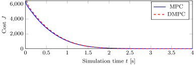
Figure 4: Global cost trajectory of the scalable spring-mass system with $40\times 40$ agents for the central MPC and DMPC case.

5.2 Plug-and-play

The plug-and-play capability of GRAMPC-D is presented using an exemplary setup of a smart grid. The network is described by a set of coupled agents that represent non-controllable power sinks and sources, such as private households, industry or renewable energy as well as controllable power plants. The dynamical behavior of the agents is generalized by describing them as generators with a mechanical phase angle $\theta_{i}(t)\in\mathbb{R}$ that may differ from the phase of the grid. The corresponding dynamics

$$\ddot{\phi}_{i}= \ \frac{1}{I\Omega}\left(u_{i}+P_{\text{source},i}-\kappa\Omega^{2}\right)-2\frac{\kappa}{I}\dot{\phi}-\sum_{j\in\mathcal{N}_{i}^{\leftarrow}}\frac{P_{\text{max},ij}}{I\Omega}\sin\left(\phi_{j}-\phi_{i}\right)$$ (30)

Figure 5: The plug-and-play capability of GRAMPC-D is presented using the simulation of a smart grid. At the beginning of the simulation, only one power sink is connected to the power plant. During run-time, the second power sink is connected to the first one, i.e. the power plant has to supply both using the same connection.

with friction constant $\kappa>0$ and the moment of inertia $I$ is given in a neighbor-affine form and describes the dynamical behavior of the phase shift $\phi_{i}(t)\in\mathbb{R}$ given by

$$\phi_{i}=\theta_{i}-\Omega\tau$$ (31)

between the phase $\Omega\tau$ of the grid with frequency $\Omega$ and the mechanical angle $\theta_{i}$, see bib:rohden2012 . Hence, the state vector is given by

$$\boldsymbol{x}_{i}= \ \begin{bmatrix}\phi_{i}&\dot{\phi}_{i}\end{bmatrix}^{\mathsf{T}}.$$ (32)

In (30), $P_{\text{source},i}$ describes the generalized non-controllable power, e.g. the demanded power for private households and industry or the generated power by renewable energy. The coupling between two agents consists of the maximum transferable power $P_{\text{max},ij}$ that depends on the phase shift angle $\phi_{j}-\phi_{i}$ between agent $i\in\mathcal{V}$ and its neighbors $j\in\mathcal{N}_{i}^{\leftarrow}$. Agents that describe power plants have a controllable input $u_{i}$ that is used to stabilize the grid. A normalized parameterization is used with $\Omega=$1\text{\,}\mathrm{Hz}$$ and $I=$1\text{\,}\mathrm{J}\text{\,}{\mathrm{s}}^{2}$$, the friction term set to $\kappa=$1\text{\times}{10}^{-3}\text{\,}\mathrm{J}\text{\,}\mathrm{s}$$ and the maximum transferable power to $P_{\text{max},ij}=$0.1\text{\,}\mathrm{J}\text{\,}{\mathrm{s}}^{-1}$$. The weighting matrices are set to

$$\boldsymbol{P}_{i}= \ \mathrm{diag}\left[$0\text{\,}{\mathrm{s}}^{2}$,$0.1\text{\,}{\mathrm{s}}^{4}$\right]\,, \boldsymbol{Q}_{i}= \ \mathrm{diag}\left[$0\text{\,}{\mathrm{s}}^{2}$,$1\text{\,}{\mathrm{s}}^{4}$\right]\,, \boldsymbol{R}_{i}= 0.01\text{\,}{\mathrm{s}}^{2}\text{\,}{\mathrm{J}}^{-2}$$ (33)

with the desired state

$$\boldsymbol{x}_{i,\text{des}}=\begin{bmatrix}\times&$0\text{\,}{\mathrm{s}}^{-2}$\end{bmatrix}^{\mathsf{T}}.$$ (34)

The first element of the desired state $\boldsymbol{x}_{i,\text{des}}$ is set arbitrary, as there is no desired value for the phase and the first state is not weighted in the cost functional.

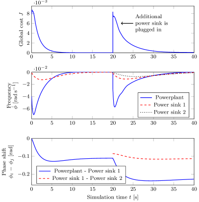
Figure 6: The Plug-and-play functionality of GRAMPC-D for the smart grid example is shown. The plot at the top shows the trajectory of the global cost, the plot in the middle the frequencies of the single agents and the plot in the bottom the phase shift between the agents. The additional power sink is plugged in at simulation time $t=$20\text{\,}\mathrm{s}$$.

The implemented setup is visualized in Figure 5. At the start of the simulation, one power plant is given that supplies one non-controllable power-sink such as a private household. During run-time, an additional power sink is coupled to the first one, i.e. the power plant has to supply both using the same connection. The simulation results are shown in Figure 6, starting with the first power sink that is connected to the power plant. It can be seen that the phase difference between the power plant and the household converges to a stationary value that leads to a transmission of the demanded power. Furthermore, the angular velocity of the phase shift converges to zero. At simulation time $t=$20\text{\,}\mathrm{s}$$, the second power sink is plugged in, leading to an additional power demand. Consequently, the phase shift between the power plant and the first power sink increases and the additional power is transmitted. The phase shift between the first and second power sink is adapted accordingly. The computation time for the distributed controller is given by a maximum of $84.67\text{\,}\mathrm{ms}$ and an average of $4.78\text{\,}\mathrm{ms}$ per agent using a step size of $\Delta_{t}=$100\text{\,}\mathrm{ms}$$. The average time is significantly lower due to the convergence criterion of the $\mathrm{ADMM}$ algorithm.

This plug-in and plug-out functionality of agents is supported at any moment during the simulation even if the controllers run on distributed hardware and communicate over a network. GRAMPC-D can handle planned changes in the system such as shown in this simulation example as well as spontaneous disconnections due to a broken network connection.

5.3 Neighbor approximation

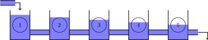
Figure 7: The concept of neighbor approximation is shown at a simulation example of coupled water tanks. Only the first one has an input and only the last one has a desired water height while being disturbed by a constant outflow.

The concept of neighbor approximation is evaluated for a system of water tanks that are coupled by pipes, see Figure 7. Only the first water tank has a controllable input $u_{1}(t)\in\mathbb{R}$. The last water tank has a constant outflow $d_{5}=$0.01\text{\,}{\mathrm{m}}^{3}\text{\,}{\mathrm{s}}^{-1}$$ and the desired water height $x_{5,des}=$3\text{\,}\mathrm{m}$$. In addition, the inequality constraint $h_{i}\leq$3\text{\,}\mathrm{m}$$ of a maximum water height has to be satisfied by all tanks. The dynamics of each water tank is given by

$$\dot{h}_{i}= \ \frac{1}{A_{i}}\left(u_{i}-d_{i}\right)+\sum_{j\in\mathcal{N}_{i}^{\leftarrow}}\frac{a_{ij}}{A_{i}}\mathrm{sign}\left(h_{j}-h_{i}\right)\sqrt{2g\left|h_{j}-h_{i}\right|}$$ (35)

with the water height $h_{i}(t)\in\mathbb{R}$ and the state vector $x_{i}=h_{i}$. The area of each water tank is given by $A_{i}=$0.1\text{\,}{\mathrm{m}}^{2}$$ and the diameter of the pipes by $a_{ij}=$0.005\text{\,}{\mathrm{m}}^{2}$$. The weights for the cost functions are set to

$$P_{1}= \ $0\text{\,}{\mathrm{m}}^{-2}$, Q_{1}= \ $0\text{\,}{\mathrm{m}}^{-2}$, R_{1}= 0.1\text{\,}{\mathrm{s}}^{2}\text{\,}{\mathrm{m}}^{-6}$$ (36a)

$$P_{i}= \ $0\text{\,}{\mathrm{m}}^{-2}$, Q_{i}= \ $0\text{\,}{\mathrm{m}}^{-2}$, R_{i}= \ $0\text{\,}{\mathrm{s}}^{2}\text{\,}{\mathrm{m}}^{-6}$,\quad i\in\{2,3,4\}$$ (36b)

$$P_{5}= \ $1\text{\,}{\mathrm{m}}^{-2}$, Q_{5}= \ $1\text{\,}{\mathrm{m}}^{-2}$, R_{5}= \ $0\text{\,}{\mathrm{s}}^{2}\text{\,}{\mathrm{m}}^{-6}$.$$ (36c)

The simulation is run with a distributed controller both with and without neighbor approximation using the same set of parameters for the $\mathrm{ADMM}$ algorithm and GRAMPC. The convergence of the $\mathrm{ADMM}$  algorithm is shown in Figure 8 for both simulations. The simulation with neighbor approximation converges smoothly to the optimal solution and satisfies the convergence criterion after $7$ iterations while $89$ $\mathrm{ADMM}$ iterations are required without neighbor approximation. Note that the cost is rising instead of falling as the solution is infeasible until the algorithm converges. The improved convergence behavior with neighbor approximation comes with a higher computational complexity per $\mathrm{ADMM}$ iteration. However, if a convergence criterion is used, the decreased number of $\mathrm{ADMM}$ iterations per time step compensate for the higher computational complexity. The required computation time for the $89$ $\mathrm{ADMM}$ iterations without neighbor approximation is $955.6\text{\,}\mathrm{ms}$ and for the $7$ iterations using neighbor approximation $203.8\text{\,}\mathrm{ms}$. Note that the same configuration for the $\mathrm{ADMM}$ algorithm and GRAMPC is used in this evaluation to provide a comparable result. The standard $\mathrm{ADMM}$ algorithm may converge within less iterations if more computation effort is spent per iteration while the algorithm may require even less time if the parameters are tuned for neighbor approximation.

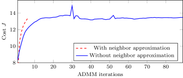
Figure 8: Convergence behavior of the $\mathrm{ADMM}$ algorithm with and without neighbor approximation. The algorithm converges within $89$ $\mathrm{ADMM}$ iterations without neighbor approximation opposed to $7$ iterations if neighbor approximation is used.

5.4 Distributed hardware implementation

This section shows the capability of GRAMPC-D to solve the $\mathrm{ADMM}$ algorithm on distributed embedded hardware. The following simulation is run on four Raspberry Pi $3\mathrm{B}+$ using Raspberry Pi OS that are connected via Ethernet. Each agent runs on an individual Raspberry Pi while the coordinator and the simulator use the same hardware. The local communication interface from GRAMPC-D based on the TCP protocol is used. The simulation example consists of three coupled Van der Pol oscillators bib:barron2009

$$\ddot{p}_{i}= \ \alpha_{1}\left(1-p_{i}^{2}\right)-p_{i}+u_{i}+\sum_{j\in\mathcal{N}_{i}^{\leftarrow}}\alpha_{2}\left(p_{j}-p_{i}\right)$$ (37)

with state $p_{i}(t)\in\mathbb{R}$, control $u_{i}(t)\in\mathbb{R}$, the uncoupled oscillator constant $\alpha_{1}=$1\text{\,}{\mathrm{m}}^{-1}\text{\,}{\mathrm{s}}^{-2}$$, and the coupling constant $\alpha_{2}=$1\text{\,}{\mathrm{s}}^{-2}$$. The state vector and desired state are given by

$$\boldsymbol{x}_{i}= \ \begin{bmatrix}p_{i}&\dot{p}_{i}\end{bmatrix}^{\mathsf{T}}$$ (38a)

$$\boldsymbol{x}_{i,\text{des}}= \ \begin{bmatrix}$0\text{\,}\mathrm{m}$&$0\text{\,}\mathrm{m}\text{\,}{\mathrm{s}}^{-1}$\end{bmatrix}^{\mathsf{T}}$$ (38b)

with the weighting matrices set to

$$\boldsymbol{P}_{i}= \ \mathrm{diag}\begin{bmatrix}$1\text{\,}{\mathrm{m}}^{-2}$&$1\text{\,}{\mathrm{m}}^{-2}\text{\,}{\mathrm{s}}^{2}$\end{bmatrix},$$ (39a)

$$\boldsymbol{Q}_{i}= \ \mathrm{diag}\begin{bmatrix}$1\text{\,}{\mathrm{m}}^{-2}$&$1\text{\,}{\mathrm{m}}^{-2}\text{\,}{\mathrm{s}}^{2}$\end{bmatrix},$$ (39b)

$$R_{i}= \ $0.1\text{\,}{\mathrm{m}}^{-2}\text{\,}{\mathrm{s}}^{4}$.$$ (39c)

The simulation is run for $10.000$ time steps using a fixed number of $q_{\text{max}}=5$ $\mathrm{ADMM}$ iterations.

Figure 9 shows the required time for computation and communication in each time step. The computation time to execute $5$ $\mathrm{ADMM}$ iterations amounts to $10\text{\,}\mathrm{ms}$ per agent while the average time required to solve the $\mathrm{ADMM}$ algorithm in a distributed manner using the TCP protocol for the communication is $66.51\text{\,}\mathrm{ms}$. Hence, the average effort for the communication is $56.51\text{\,}\mathrm{ms}$ including $72$ communication steps. Since all agents have to be synchronized for the $\mathrm{ADMM}$ algorithm, either of them has to wait for the slowest agent at each step of the algorithm. All five $\mathrm{ADMM}$ iterations can be executed in $48\text{\,}\mathrm{ms}$ with the worst case time of $114\text{\,}\mathrm{ms}$. This results in the minimum time for each communication step of $0.53\text{\,}\mathrm{ms}$, an average time of $0.79\text{\,}\mathrm{ms}$ and a maximum time of $1.44\text{\,}\mathrm{ms}$. This time includes preparing the data to be sent, sending and receiving it and recreating the sent data structure from the byte array. These are plausible values as a ping to the loopback address $127.0.0.1$ already requires $0.14\text{\,}\mathrm{ms}$ in average and $0.22\text{\,}\mathrm{ms}$ at maximum. These results show that the main effort in distributed optimization is the communication effort that requires $82.3\%$ of the overall time in average for this simulation example.

Figure 9: Communication effort of the $\mathrm{ADMM}$ algorithm on distributed hardware with $48\text{\,}\mathrm{ms}$ (minimum), $66.51\text{\,}\mathrm{ms}$ (average), and $114\text{\,}\mathrm{ms}$ (maximum) compared to the computation time of $10\text{\,}\mathrm{ms}$.

6 Conclusions

The open-source, modular DMPC framework GRAMPC-D is presented in this paper that enables to solve scalable optimal control problems in a convenient way and to stabilize plants using distributed model predictive control. This problem description can be used for both a centralized and a distributed controller. In the distributed setting, the global optimal control problem is automatically decoupled and solved in a distributed manner using the $\mathrm{ADMM}$  algorithm. The convergence behavior of the $\mathrm{ADMM}$  algorithm can be improved by sugint he concept of neighbor approximation that allows the agents to anticipate the actions of their neighbors. The presented DMPC framework supports plug-and-play to connect and remove agents at run-time. Besides solving the $\mathrm{ADMM}$ algorithm on a single processor, it is possible to solve the local optimal control problems on distributed hardware. The local communication interface enables communication between agents over a network using the TCP protocol. By default, GRAMPC-D uses the MPC toolbox GRAMPC for solving the local optimal control problems on agent level, which is suitable for real-time and embedded implementations.

GRAMPC-D is licensed under the Berkeley Software Distribution 3-clause version (BSD-3) license. The complete source-code is available at Github https://github.com/grampc-d/grampc-d. Future work will use the modular structure to extend GRAMPC-D. For example, communication protocols besides TCP can be provided or alternative solvers to GRAMPC for the underlying minimization problem implemented to increase the usability and flexibility of the framework.

References

• (1) D. Mayne, J. Rawlings, C. Rao, and P. Scokaert, “Constrained model predictive control: stability and optimality,” Automatica, vol. 36, no. 6, pp. 789–814, 2000.
• (2) F. Allgöwer and A. Zheng, Nonlinear model predictive control.   Birkhäuser, 2012, vol. 26.
• (3) B. Houska, H. J. Ferreau, and M. Diehl, “ACADO toolkit - an open-source framework for automatic control and dynamic optimization,” Optimal Control Applications and Methods, vol. 32, pp. 298–312, 2011.
• (4) R. Verschueren, G. Frison, D. Kouzoupis, N. van Duijkeren, A. Zanelli, B. Novoselnik, J. Frey, T. Albin, R. Quirynen, and M. Diehl, “acados: a modular open-source framework for fast embedded optimal control,” arXiv preprint arXiv:1910.13753, 2019.
• (5) J. Kalmari, J. Backman, and A. Visala, “A toolkit for nonlinear model predictive control using gradient projection and code generation,” Control Engineering Practice, vol. 39, pp. 56–66, 2015.
• (6) B. Käpernick and K. Graichen, “The gradient based nonlinear model predictive control software grampc,” in Proc. ECC, 2014, pp. 1170–1175.
• (7) T. Englert, A. Völz, F. Mesmer, S. Rhein, and K. Graichen, “A software framework for embedded nonlinear model predictive control using a gradient-based augmented Lagrangian approach (GRAMPC),” Optimization and Engineering, vol. 20, no. 3, pp. 769–809, 2019.
• (8) E. Camponogara, D. Jia, B. Krogh, and S. Talukdar, “Distributed model predictive control,” IEEE Control Systems Magazine, vol. 22, no. 1, pp. 44–52, 2002.
• (9) J. M. Maestre and R. R. Negenborn, Distributed Model Predictive Control Made Easy.   Springer, 2014.
• (10) H. Scheu and W. Marquardt, “Sensitivity-based coordination in distributed model predictive control,” Journal of Process Control, vol. 21, no. 5, pp. 715–728, 2011.
• (11) B. Houska, J. Frasch, and M. Diehl, “An augmented Lagrangian based algorithm for distributed nonconvex optimization,” SIAM Journal on Optimization, vol. 26, no. 2, pp. 1101–1127, 2016.
• (12) B. Houska, D. Kouzoupis, Y. Jiang, and M. Diehl, “Convex optimization with ALADIN,” Math. Program., 2018.
• (13) S. Boyd, N. Parikh, E. Chu, B. Peleato, and J. Eckstein, “Distributed optimization and statistical learning via the alternating direction method of multipliers,” Foundations and Trends in Machine Learning, vol. 3, no. 1, 2011.
• (14) O. Gäfvert, “A Practical Guide to Distributed Model Predictive Control,” 2014. [Online]. Available: github.com/olivergafvert/dmpc
• (15) S. Riverso, A. Battocchio, and G. Ferrari-Trecate, “PnPMPC toolbox,” 2013. [Online]. Available: http://sisdin.unipv.it/pnpmpc/pnpmpc.php
• (16) F. Farina, A. Camisa, A. Testa, I. Notarnicola, and G. Notarstefano, “DISROPT: a Python Framework for Distributed Optimization,” arXiv preprint arXiv:1911.02410, 2019.
• (17) A. Engelmann, Y. Jiang, H. Benner, R. Ou, B. Houska, and T. Faulwasser, “ALADIN-$\alpha$ – An open-source MATLAB toolbox for distributed non-convex optimization,” arXiv preprint arXiv:2006.01866, 2020.
• (18) W. Jakob, J. Rhinelander, and D. Moldovan, “pybind11 – Seamless operability between C++11 and Python,” 2017, https://github.com/pybind/pybind11.
• (19) S. Hentzelt and K. Graichen, “An augmented Lagrangian method in distributed dynamic optimization based on approximate neighbor dynamics,” in Proc. of IEEE SMC, Manchester (United Kingdom), 2013, pp. 571–576.
• (20) G. Filatrella, A. H. Nielsen, and N. F. Pedersen, “Analysis of a power grid using a kuramoto-like model,” The European Physical Journal B, vol. 61, no. 4, pp. 485–491, 2008.
• (21) A. Bestler and K. Graichen, “Distributed model predictive control for continuous-time nonlinear systems based on suboptimal ADMM,” Optimal Control Applications and Methods, vol. 40, pp. 1–23, 2019.
• (22) D. P. Bertsekas, Constrained optimization and Lagrange multiplier methods.   Academic press, Belmont, 1996.
• (23) D. Burk, A. Völz, and K. Graichen, “Neighbor Approximations for Distributed Optimal Control of Nonlinear Networked Systems,” in Proc. of ECC, St. Petersburg (Russia), 2020, pp. 1238–1243.
• (24) M. Zeilinger, Y. Pu, S. Riverso, G. Ferrari-Trecate, and C. Jones, “Plug and play distributed model predictive control based on distributed invariance and optimization,” in Proc. of 52nd IEEE CDC, Florence (Italia), Dec. 2013, pp. 5770–5776.
• (25) S. Riverso, M. Farina, and G. Ferrari-Trecate, “Plug-and-play model predictive control based on robust control invariant sets,” Automatica, vol. 50, no. 8, pp. 2179–2186, 2014.
• (26) S. Riverso and G. Ferrari-Trecate, “Plug-and-play distributed model predictive control with coupling attenuation,” Optimal Control Applications and Methods, vol. 36, no. 3, pp. 292–305, 2015.
• (27) D. Burk, A. Völz, and K. Graichen, “Towards a Modular Framework for Distributed Model Predictive Control of Nonlinear Neighbor-Affine Systems,” in Proc. of 58th IEEE CDC, Nice (France), 2019, pp. 5279–5284.
• (28) M. Rohden, A. Sorge, M. Timme, and D. Witthaut, “Self-organized synchronization in decentralized power grids,” Physical Review Letters, vol. 109, no. 6, pp. 064 101–1 – 064 101–5, 2012.
• (29) M. A. Barrón and M. Sen, “Synchronization of four coupled van der Pol oscillators,” Nonlinear Dynamics, vol. 56, no. 4, pp. 357–367, 2009.