Abstract

The classical approach to measure the expressive power of deep neural networks with piecewise linear activations is based on counting their maximum number of linear regions. This complexity measure is quite relevant to understand general properties of the expressivity of neural networks such as the benefit of depth over width. Nevertheless, it appears limited when it comes to comparing the expressivity of different network architectures. This lack becomes particularly prominent when considering permutation-invariant networks, due to the symmetrical redundancy among the linear regions. To tackle this, we propose a refined definition of piecewise linear function complexity: instead of counting the number of linear regions directly, we first introduce an equivalence relation among the linear functions composing a piecewise linear function and then count those linear functions relative to that equivalence relation. Our new complexity measure can clearly distinguish between the two aforementioned models, is consistent with the classical measure, and increases exponentially with depth.

1 Introduction

Deep neural networks with rectified linear units (ReLU) as an activation function have been remarkably successful in computer vision, speech recognition, and other domains (Alex et al.,, 2012), (Goodfellow et al.,, 2013), (Wan et al.,, 2013), (Silver et al.,, 2017). However, the theoretical understanding to support this experimental progress is still insufficient, thereby motivating several researchers to bridge this crucial gap.

A fundamental theoretical problem is the expressivity of neural networks: given an architecture configuration (depth, width, layer type, activation function), which class of functions can neural networks compute and with what level of performance? To evaluate the expressive power of a neural network, we, therefore, need to define a measure of its complexity. In the case where ReLU is the only considered activation function, a neural network represents a piecewise linear function, thus, a natural method to measure complexity is to count the number of linear regions. From this perspective, we can theoretically justify favoring depth over width. Moreover, this has also been widely established through experimentation (Pascanu et al.,, 2013), (Montúfar et al.,, 2014), (Telgarsky,, 2016), (Arora et al.,, 2016), (Eldan and Shamir,, 2016), (Yarotsky,, 2017), (Serra et al.,, 2018), (Chatziafratis et al.,, 2019), (Chatziafratis et al.,, 2020).

Nevertheless, as we subsequently show, using the number of linear regions as a straightforward measure, does not adequately reflect the properties of the underlying function which the network represents in some case.

Concretely, we consider permutation-invariant functions and the model introduced by Zaheer et al., (2017). This model has been proven to be a universal approximator for the class of permutation-invariant continuous functions (Maron et al.,, 2019), (Zaheer et al.,, 2017). Since this model is permutation-invariant, its expressive power is strictly lower than that of the fully connected model. However, we point out that the maximal number of linear regions for both the models is asymptotically similar.

This highlights the fact that the straightforward relationship between number of linear regions and expressive power needs to be qualified, because it cannot distinguish between these two models clearly. Thus, we propose a new complexity measure that enables us to reliably make this distinction.

Our main contribution is to introduce such a measure (Definition 2) and to prove that the invariant model and the fully connected model actually have different values (Theorem 1, Theorem 3). To define our measure, we consider not the number of linear regions but the number of linear functions on them. Our measure counts them relative to a certain equivalence relation. This relation identifies linear functions (and their inherent linear region) that can be mapped from one to another through a certain Euclidean transformation, i.e., isometric affine transformation. As a more intrinsic example, we consider digital images. The complexity of digital images is usually estimated by the number of pixels and the number of colors. The number of pixels corresponds to the conventional measure of complexity, i.e., the number of linear regions $c^{\#}$, and the number of colors corresponds to our proposed measure of complexity, i.e., the number of linear functions $c^{\sim}$. From this point of view, our measure is a natural consequence. We remark that other possible measures of complexity such as using Betti numbers of the linear regions (Bianchini and Scarselli,, 2014), trajectories in the input space (Raghu et al.,, 2017), or the volumes of the boundaries of linear regions (Hanin and Rolnick,, 2019) have been proposed.

The low expressive power of permutation-invariant shallow networks is translated to the fewness of linear functions ($\approx$“colors”) composing them, due to permutation invariance. Indeed, we show that for permutation-invariant shallow models, the proposed measure of complexity is the same as the number of orbits of linear regions by permutation action and that this number is relatively small. Our demonstration relies on theory of hyperplane arrangement which is stable by group action studied in (Kamiya et al.,, 2012). In Section 4, we modified the argument of Montúfar et al., (2014) to prove the benefit of depth over width. Particularly, the complexity of the proposed method increases exponentially with depth for fully connected deep models as well as for permutation-invariant deep models introduced by Zaheer et al., (2017).

2 Preliminaries and background

A (feedforward) neural network of depth $L+1$ is a composition of layers of units which defines a function $F\colon\mathbb{R}^{n_{0}}\to\mathbb{R}^{n_{L+1}}$ of the form

$$F(\bm{x})=f_{L+1}\circ g_{L}\circ f_{L}\circ\cdots\circ g_{1}\circ f_{1}(\bm{x}),$$ (2.1)

where $f_{l}\colon\mathbb{R}^{n_{l-1}}\to\mathbb{R}^{n_{l}}$ is an affine map and $g_{l}\colon\mathbb{R}^{n_{l}}\to\mathbb{R}^{n_{l}}$ is a nonlinear activation function. Throughout this paper, as activation functions, we consider the rectifier linear units (ReLU), i.e., for $\bm{x}=(x_{1},\dots,x_{n_{l}})^{\top}\in\mathbb{R}^{n_{l}}$,

$$\mathrm{ReLU}\ \!(\bm{x})=(\max\{0,x_{1}\},\dots,\max\{0,x_{n_{l}}\})^{\top}\in\mathbb{R}^{n_{l}}.$$

Let $\underline{n}=(n_{0},n_{1},\dots,n_{L+1})$ and $K$ be a connected compact $n_{0}$-dimensional subset of $\mathbb{R}^{n_{0}}$. Then, we define $\mathcal{H}_{K}^{\text{full}}(\underline{n})=\mathcal{H}_{K}^{\text{full}}(n_{0},n_{1},\dots,n_{L+1})$ as the set of the restriction to $K$ of the neural networks of the form (2.1) with $g_{l}=\mathrm{ReLU}\ \!$ for any $l=1,\dots,L$. We call such a network a ReLU neural network. The affine transformation $f_{l}$ can be written as $f_{l}(\bm{x})=W_{l}\bm{x}+\bm{c}_{l}$ with a weight matrix $W_{l}\in\mathbb{R}^{n_{l}\times n_{l-1}}$ and a bias vector $\bm{c}_{l}\in\mathbb{R}^{n_{l}}$. We call the feedforward neural network shallow (resp. deep) if $L=1$ (resp. $L>1$).

Because $\mathrm{ReLU}\ \!$ is a continuous piecewise linear function, a function realized by a ReLU neural network is also continuous and piecewise linear. We are interested in the structures of such piecewise linear functions. Any piecewise linear function is encoded as the set of pairs made of a linear region and a linear function on it. Here, for a connected compact $m$-dimensional subset $K$ in $\mathbb{R}^{m}$ and a piecewise linear function $f\colon K\to\mathbb{R}^{n}$, a connected region $D\subset K$ is called a linear region of $f$ if $f$ is linear on $D$ and for any connected region $D^{\prime}\subset K$ satisfying $D\subsetneq D^{\prime}$, $f$ is not linear on $D^{\prime}$. For a piecewise linear function $f$, $c^{\#}(f)$ denotes the number of linear regions of $f$. For a set of piecewise linear functions $\mathcal{H}$, we set $c^{\#}(\mathcal{H})=\max\{c^{\#}(f)\mid f\in\mathcal{H}\}$.

2.1 The number of linear regions for shallow fully connected neural networks

To calculate the maximum number of linear regions for shallow ReLU neural networks, we use arguments from hyperplane arrangement theory as in (Pascanu et al.,, 2013). Let us consider a shallow ReLU neural network $F\in\mathcal{H}_{K}^{\text{full}}(n_{0},n_{1},n_{2})$, i.e., a network of the form

$$F(\bm{x})=f_{2}\circ g_{1}\circ f_{1}(\bm{x}),$$ (2.2)

where $f_{1}\colon K\to\mathbb{R}^{n_{1}}$ and $f_{2}\colon\mathbb{R}^{n_{1}}\to\mathbb{R}^{n_{2}}$ are two affine maps and $g_{1}\colon\mathbb{R}^{n_{1}}\to\mathbb{R}^{n_{1}}$ is ReLU.

The linear regions of $F$ depend only on the affine map $f_{1}$. We write $f_{1}(\bm{x})=W\bm{x}+\bm{c}$ for $W=(a_{ij})\in\mathbb{R}^{n_{1}\times n_{0}}$ and $\bm{c}=(c_{i})\in\mathbb{R}^{n_{1}}$. Let $H_{i}$ be the hyperplane in $\mathbb{R}^{n_{0}}$ defined as

$$a_{i1}x_{1}+\cdots+a_{in_{0}}x_{n_{0}}+c_{i}=0\ \cdots\ H_{i}$$

for $i=1,\dots,n_{1}$. Then, the linear regions of $F$ are exactly the chambers of the hyperplanes arrangement defined by $\mathcal{A}=\{H_{1},\dots,H_{n_{1}}\}$, i.e., the connected components of the complement $\mathbb{R}^{n_{0}}{\setminus}\bigcup_{i}H_{i}$. Let ${\rm Ch}(\mathcal{A})$ denotes the set of chambers of arrangement $\mathcal{A}$. Then, Schläfli showed that the cardinality $|{\rm Ch}(\mathcal{A})|$ of ${\rm Ch}(\mathcal{A})$ satisfies

$$|{\rm Ch}(\mathcal{A})|\leq\sum_{i=0}^{n_{0}}{n_{1}\choose i}$$ (2.3)

and the equality holds if $\mathcal{A}$ is in general position (Orlik and Terao,, 2013, Introduction). Here, we say that the hyperplane arrangement $\mathcal{A}=\{H_{1},\dots,H_{n_{1}}\}$ is in general position if $\mathcal{A}$ satisfies that for any $r=1,\dots,n_{0}$, the codimension of the intersection $H_{i_{1}}\cap\cdots\cap H_{i_{r}}$ is equal to $r$ if $r\leq n_{1}$ and $H_{i_{1}}\cap\cdots\cap H_{i_{r}}=\emptyset$ if $r>n_{1}$ (see Appendix A.1 for an illustration). For the hyperplane arrangement $\mathcal{A}$ defined by the fully connected shallow neural network above, we remark that it is always possible to make it being in general position by perturbing the weight matrix $W$ and the bias vector $\bm{c}$. Moreover, for any connected compact $n_{0}$-dimensional subset $K\subset\mathbb{R}^{n_{0}}$ and a hyperplane arrangement $\mathcal{A}$, we can take another hyperplane arrangement $\mathcal{A}^{\prime}=\{H_{i}^{\prime}\mid i=1,\dots,n_{1}\}$ such that $|{\rm Ch}(\mathcal{A})|$ is equal to the number of connected components of $K{\setminus}\bigcup_{i}(K\cap H_{i}^{\prime})$ by translating or scaling $\mathcal{A}$ if it is necessary. In particular, the maximal number $c^{\#}(\mathcal{H}_{K}^{\mathrm{full}}(n_{0},n_{1},n_{2}))$ of linear regions of the fully connected shallow ReLU neural network having a $n_{0}$-dimensional input layer and a $n_{1}$-dimensional hidden layer is $\sum_{i=0}^{n_{0}}{n_{1}\choose i}$. For $n_{0}$ such that $0\leq n_{0}\leq n_{1}/2$, by (Ash,, 1965, Section 4.7), the estimate of the sum of binomial coefficients is

$$\frac{2^{n_{1}H(n_{0}/n_{1})}}{\sqrt{8n_{0}(1-n_{0}/n_{1})}} \leq{n_{1}\choose n_{0}}\leq c^{\#}(\mathcal{H}_{K}^{\mathrm{full}}(n_{0},n_{1},n_{2}))$$

$$=\sum_{i=0}^{n_{0}}{n_{1}\choose i}\leq 2^{n_{1}H(n_{0}/n_{1})},$$ (2.4)

where $H(p)$ is the binary entropy function defined as

$$H(p)=-p\log_{2}p-(1-p)\log_{2}(1-p)$$

for $0<p<1$ and $H(0)=H(1)=0$.

2.2 The number of linear regions for the permutation invariant model

We review the permutation invariant shallow model introduced in (Zaheer et al.,, 2017) and show that this model can have as many linear regions as a fully connected shallow neural network, though this model has a lower expressive power than the fully connected model. We illustrate this calculation on a simple example in Appendix A.2.

We define the permutation action on $(\mathbb{R}^{n})^{m}$ of permutation group $S_{n}$ by the following way. For $\sigma\in S_{n}$ and $\bm{X}=(\bm{x}_{1},\dots,\bm{x}_{m})\in(\mathbb{R}^{n})^{m}$ where $\bm{x}_{i}=(x_{i1},\dots,x_{in})^{\top}\in\mathbb{R}^{n}$, we define

$$\sigma\cdot\bm{X} =(\sigma\cdot\bm{x}_{1},\dots,\sigma\cdot\bm{x}_{n}),$$

$$\sigma\cdot\bm{x}_{i} =(x_{i\sigma^{-1}(1)},\dots,x_{i\sigma^{-1}(n)})^{\top}.$$

For a subset $K$ of $\mathbb{R}^{n}$, we say that $K$ is stable by permutation action if for any $\bm{x}\in K$, $\sigma\cdot\bm{x}\in K$ holds for any $\sigma\in S_{n}$.

We consider a permutation invariant shallow network as

$$F(\bm{x})=f_{2}\circ g_{1}\circ f_{1}(\bm{x})$$ (2.5)

where $f_{1}\colon\mathbb{R}^{n}\to(\mathbb{R}^{n})^{m}$ is a permutation equivariant affine map, i.e., $f_{1}(\sigma\cdot\bm{x})=\sigma\cdot f_{1}(\bm{x})$ for any $\sigma\in S_{n}$ and $\bm{x}\in\mathbb{R}^{n}$, and $f_{2}\colon(\mathbb{R}^{n})^{m}\to\mathbb{R}^{m^{\prime}}$ is a permutation invariant affine map i.e., $f_{2}(\sigma\cdot\bm{X})=f_{2}(\bm{X})$ for any $\bm{X}\in(\mathbb{R}^{n})^{m}$ and $\sigma\in S_{n}$, and $g_{1}\colon(\mathbb{R}^{n})^{m}\to(\mathbb{R}^{n})^{m}$ is ReLU. Then, the realized function $F$ is permutation invariant, i.e., $F(\sigma\cdot\bm{x})=F(\bm{x})$ for any $\sigma\in S_{n}$. Let $K$ be a connected compact $n$-dimensional subset of $\mathbb{R}^{n}$ which is stable by permutation action. Then, we define $\mathcal{H}_{K}^{\text{inv}}(n,mn,m^{\prime})$ as the set of the restrictions to $K$ of the permutation invariant ReLU neural networks of the form (2.5). By universal approximation theorem (Maron et al.,, 2019), any permutation-invariant, continuous function on $K$ can be approximated by such a neural networks for large enough $m^{\prime}$.

The set of linear regions of the model depends only on the affine map $f_{1}$ as in the fully connected case. Using (Zaheer et al.,, 2017, Lemma 3), by the permutation equivariance of $f_{1}$, if we set $f_{1}(\bm{x})=W\bm{x}+\bm{c}$ for some $W\in(\mathbb{R}^{n\times n})^{m}$ and $\bm{c}\in(\mathbb{R}^{n})^{m}$, these $W$ and $\bm{c}$ can be written as

$$W=\begin{pmatrix}a_{1}I+b_{1}(I-\bm{1}\bm{1}^{\top})\\ \vdots\\ a_{m}I+b_{m}(I-\bm{1}\bm{1}^{\top})\end{pmatrix},\ \bm{c}=\begin{pmatrix}c_{1}\bm{1}\\ \vdots\\ c_{m}\bm{1}\end{pmatrix}$$ (2.6)

for some $a_{1},\dots,a_{m},b_{1},\dots,b_{m},c_{1},\dots,c_{m}\in\mathbb{R}$. Here, $I$ is the identity matrix in $\mathbb{R}^{n\times n}$ and $\bm{1}$ is the all one vector in $\mathbb{R}^{n}$. Thus, the set of linear regions of $F$ is equal to the set of chambers of the hyperplanes arrangement $\mathcal{B}_{m,n}=\{H_{11},\dots,H_{mn}\}$ defined for $i=1,\dots,m$ by,

$$\begin{cases}a_{i}x_{1}+b_{i}x_{2}+\cdots+b_{i}x_{n}+c_{i}=0&\ \cdots\ H_{i1}\\ b_{i}x_{1}+a_{i}x_{2}+\cdots+b_{i}x_{n}+c_{i}=0&\ \cdots\ H_{i2}\\ \hskip 80.0pt\vdots&\\ b_{i}x_{1}+b_{i}x_{2}+\cdots+a_{i}x_{n}+c_{i}=0&\ \cdots\ H_{in}.\end{cases}$$ (2.7)

We calculate the number of chambers of the arrangement $\mathcal{B}_{m,n}$. As in inequation (2.3), the number of chambers are bounded from above by $\sum_{i=0}^{n}{mn\choose i}$ and attains this bound if the arrangement $\mathcal{B}_{m,n}$ is in general position. However, this arrangement $\mathcal{B}_{m,n}$ cannot be in general position. Indeed, the hyperplanes in the arrangement $\mathcal{B}_{m,n}$ satisfy

$$H_{i_{1},j}\cap H_{i_{2},j}\cap H_{i_{3},j} =\emptyset,$$ (2.8)

$$H_{i_{1},j_{1}}\cap H_{i_{1},j_{2}}\cap H_{i_{2},j_{1}} =H_{i_{1},j_{1}}\cap H_{i_{1},j_{2}}\cap H_{i_{2},j_{2}}$$

$$=H_{i_{1},j_{1}}\cap H_{i_{2},j_{1}}\cap H_{i_{2},j_{2}}$$

(2.9)

for $i_{1},i_{2},i_{3}=1,\dots,m$ and $j,j_{1},j_{2}=1,\dots,n$. Nevertheless, we can calculate the number of chambers of the arrangement $\mathcal{B}_{m,n}$ by applying the Deletion-Restriction theorem (Theorem 6 in Appendix B) (Orlik and Terao,, 2013, Theorem 2.56 and Theorem 2.68) under the assumption (2.8) and (2.9). The detail of the calculation is in Appendix B.

Proposition 1.

We assume that $m>n/2$. Then, the maximum $b_{m,n}$ of the number of chambers of $\mathcal{B}_{m,n}$ is bounded from below by a function $g(m,n)$ which is polynomial with respect to $m$ of degree $n$, and which the coefficient of the leading term is bounded from below by $(2^{5/4})^{n}/(n\sqrt{2})$.

2.3 Comparison of the numbers of linear regions

To equalize the number of hidden units in both models, we consider the fully connected model (2.2) withd $n_{0}=n$ and $n_{1}=mn$. Let $K$ be a connected compact $n$-dimensional subset of $\mathbb{R}^{n}$ which is stable by permutation action. By a universal approximation theorem (Sonoda and Murata,, 2017), if we increase the number of hidden units of the fully connected shallow models, the elements of $\mathcal{H}_{K}^{\text{full}}(n,mn,m^{\prime})$ can approximate any continuous maps on a compact set of $\mathbb{R}^{n}$. On the other hand, although elements of $\mathcal{H}_{K}^{\text{inv}}(n,mn,m^{\prime})$ are also universal approximators for permutation-invariant functions (Maron et al.,, 2019), any function which is not permutation-invariant cannot be approximated by the elements of $\mathcal{H}_{K}^{\text{inv}}(n,mn,m^{\prime})$. This implies that the expressive power of the permutation-invariant shallow models is strictly lower than for the fully connected shallow models.

In keeping with this observation, we compare maximum number of linear regions for the fully connected (2.2) and the permutation invariant shallow models (2.5). By the estimate (2.4) with $n_{0}=n$ and $n_{1}=mn$, we have

$$c^{\#}(\mathcal{H}_{K}^{\mathrm{full}})(n,mn,n^{\prime}) \geq\frac{2^{mnH(1/m)}}{\sqrt{8n(1-1/m)}}$$

$$\geq\frac{e^{n}}{2\sqrt{2n}}m^{n}+O(m^{n-1}).$$

On the other hand, by Proposition 1, the maximal number of linear regions of permutation invariant shallow models is also bounded from below as

$$c^{\#}(\mathcal{H}_{K}^{\mathrm{inv}})(n,mn,n^{\prime})\geq\frac{(2^{5/4})^{n}}{n\sqrt{2}}m^{n}+O(m^{n-1}).$$

In particular, although there is a difference of bases, $c^{\#}(\mathcal{H}_{K}^{\mathrm{inv}})(n,mn,n^{\prime})$ does also increase exponentially with respect to $n$. This means that the maximum numbers of linear regions cannot represent the difference of expressive powers of these models clearly.

This observation indicates that we should consider some refined measure for complexity and expressive power to be able to distinguish between these two classes of models more clearly.

3 Measure of complexity as the numbers of equivalent classes of linear functions

In this section, we introduce a measure of complexity which can distinguish permutation-invariant shallow models from fully connected shallow models. Before proposing a refined measure of complexity, we observe the structure of piecewise linear functions that are permutation-invariant.

Let $K$ be a connected compact $n$-dimensional subset of $\mathbb{R}^{n}$ which is stable by permutation action and $f\colon K\to\mathbb{R}^{n^{\prime}}$ be a piecewise linear function which is permutation invariant by the permutation group $S_{n}$, and $\mathcal{F}(f)=\{(f_{\lambda},D_{\lambda})\mid\lambda\in\Lambda\}$ the set of pairs of linear regions $D_{\lambda}\subset K$ of $f$ and the linear associated function $f_{\lambda}$ on $D_{\lambda}$, i.e., $f_{\lambda}$ is the restriction $f|_{D_{\lambda}}$ of $f$ on $D_{\lambda}$. We call this set $\mathcal{F}(f)$ the set of linear functions of $f$. We often abbreviate an element $(f_{\lambda},D_{\lambda})\in\mathcal{F}(f)$ to $f_{\lambda}$. Then, it is easy to show that for any permutation $\sigma\in S_{n}$ and any linear region $D$ of $f$, the image $\sigma(D)$ of $D$ by $\sigma$ is also a linear region. By this fact and the permutation invariance of $f$, for any $(f_{\lambda},D_{\lambda})$ and $\sigma\in S_{n}$, there is a $\lambda^{\prime}$ such that $\sigma(D_{\lambda})=D_{\lambda^{\prime}}$ and $f_{\lambda}=f_{\lambda^{\prime}}\circ\sigma|_{D_{\lambda}}$. Here, we regard the permutation $\sigma$ as a linear transformation on $\mathbb{R}^{n}$. Then, the linear transformation induced by permutation $\sigma$ is isometric with respect to $L^{2}$-norm, because the map taking $L^{2}$-norm $\bm{x}\mapsto\|\bm{x}\|_{2}$ is permutation-invariant.

Inspired by this observation, we define an equivalence relation $\sim$ on the set of pairs $\mathcal{F}(f)$ of linear functions and regions for piecewise linear function $f\colon K\to\mathbb{R}^{n^{\prime}}$ as follows:

Definition 1.

Let $f\colon K\to\mathbb{R}^{n^{\prime}}$ be a piecewise linear function and $\mathcal{F}(f)=\{(f_{\lambda},D_{\lambda})\mid\lambda\in\Lambda\}$ the set of the linear functions of $f$. Then, we say that $f_{\lambda}$ is equivalent to $f_{\lambda^{\prime}}$, denoted by $f_{\lambda}\sim f_{\lambda^{\prime}}$, if there is a Euclidean transformation $\phi\colon\mathbb{R}^{n}\to\mathbb{R}^{n}$ satisfying ${\rm(1)}\ \phi(D_{\lambda})=D_{\lambda^{\prime}}$ and ${\rm(2)}\ f_{\lambda}=f_{\lambda^{\prime}}\circ\phi|_{D_{\lambda}}$. Here, a Euclidean transformation $\phi$ is an affine map written as $\phi(\bm{x})=A\bm{x}+\bm{b}$ for an orthogonal matrix $A$ and a vector $\bm{b}$.

We can characterize the invariant function for a group action as follows: (the proof is in Appendix C):

Proposition 2.

Let $f$ be a piecewise linear function on $K$ and $\mathcal{F}(f)=\{(f_{\lambda},D_{\lambda})\mid\lambda\in\Lambda\}$ the set of linear functions of $f$. We assume that there is a set $\Phi=\{\phi_{1},\dots,\phi_{t}\}$ of Euclidean transformations on $\mathbb{R}^{n}$ such that for any $\phi\in\Phi$ and any linear regions $D_{\lambda}$, there is a $\lambda^{\prime}\in\Lambda$ such that ${\rm(1)}\ \phi(D_{\lambda})=D_{\lambda^{\prime}},\ \ \ \ {\rm(2)}\ f_{\lambda}=f_{\lambda^{\prime}}\circ\phi|_{D_{\lambda}}$. Then, $f$ is $\hat{\Phi}$-invariant, where $\hat{\Phi}=\langle\phi_{1},\dots,\phi_{t}\rangle$ is the group generated by $\Phi$.

The relation $\sim$ is an equivalence relation. Then, we propose the following measure of complexity:

Definition 2.

We define the measure of complexity $c^{\sim}(f)$ of $f$ by the number of equivalent classes $\mathcal{F}(f)/{\sim}$. For a set $\mathcal{H}$ of piecewise linear functions, we define the measure of complexity $c^{\sim}(\mathcal{H})$ of $\mathcal{H}$ by the maximum of $c^{\sim}(f)$ for any $f\in\mathcal{H}$.

As a trivial upper bound, $c^{\sim}(f)$ is bounded from above by $|\mathcal{F}(f)|$, i.e., the number of linear regions. More generally, the set $\mathcal{F}(f)$ of linear functions of $f$ may be infinite. However, if $f$ is realized by a ReLU neural network of finite width and finite depth, $\mathcal{F}(f)$ is finite.

We calculate this measure of complexity for the previous two classes of models. We remark that any Euclidean transformation $\phi$ does not change the volumes of linear regions. Thus, if the volumes of two linear regions $D_{\lambda}$ and $D_{\lambda^{\prime}}$ are different, then $f_{\lambda}$ and $f_{\lambda^{\prime}}$ cannot be equivalent. We use this observation later to count the number of equivalent classes.

3.1 Examples of our measure of complexity in $1$-dimensional case

Here, we show some examples in the 1-dimensional case and calculate our measures of complexity. For simplicity, we consider them on the interval $K=[0,1]$.

Let $f$ be a piecewise linear function on $[0,1]$ and $[0,1]=\bigcup_{i=1}^{m}D_{i}$ be the decomposition by linear regions $D_{i}$ for $f$ and $f_{i}=f|_{D_{i}}$. Then, $(f_{i},D_{i})\sim(f_{j},D_{j})$ holds only if $|D_{i}|=|D_{j}|$, where $|D|$ for interval $D=[p,q]$ is the length $q-p$. Indeed, by Definition 1, there is a Euclidean transformation $\phi\colon\mathbb{R}^{1}\to\mathbb{R}^{1};x\mapsto ax+b$ such that $\phi(D_{j})=D_{i}$. As $\phi$ is Euclidean transformation, $a$ is equal to $\pm 1$. If we set $D_{i}=[p_{i},q_{i}]$, then $\phi(D_{j})=D_{i}$ is equivalent to $[p_{j},q_{j}]=[\phi(p_{i}),\phi(q_{i})]=[ap_{i}+b,aq_{i}+b]$. As $a=\pm 1$, this implies that $|D_{j}|=|D_{i}|$. Moreover, then, $ap_{i}+b=p_{j}$ holds. In particular, $b=p_{j}-ap_{i}$ holds. Because $a$ is $1$ or $-1$, there are only two choices of the Euclidean transformation $\phi\colon D_{i}\to D_{j}$.

Furthermore, we set $f_{i}(x)=\alpha_{i}x+\beta_{i}$ for $i=1,\dots,m$. Then, $(f_{j}\circ\phi)|_{D_{i}}=f_{i}$ holds. Hence, for $x\in D_{i}$,

$$\alpha_{i}x+\beta_{i}=\alpha_{j}(ax+b)+\beta_{j}=a\alpha_{j}x+\alpha_{j}b+\beta_{j}$$

holds. Thus, we have $\alpha_{i}=a\alpha_{j}$ and $\beta_{i}=b\alpha_{j}+\beta_{j}$.

By combining these arguments, there are at most two linear functions on $D_{j}=[p_{j},q_{j}]$ equivalent to $(f_{i},D_{i})$ where $f_{i}(x)=\alpha_{i}x+\beta_{i}$ and $D_{i}=[p_{i},q_{i}]$: For $f_{i}(x)=\alpha_{i}x+\beta_{i}$,

$$f_{j}(x)=\begin{cases}\alpha_{i}x+\beta_{i}-(p_{j}-p_{i})\alpha_{i}&\text{if }a=1,\\ -\alpha_{i}x+\beta_{i}+(p_{j}+p_{i})\alpha_{i}&\text{if }a=-1.\end{cases}$$

Based on this observation, we show three examples on $[0,1]$.

Figure 1: Example 1	Figure 2: Example 2	Figure 3: Example 3
Figure 4: Example 4 Figure 5: Example 5

Example 1.

Let $f\colon[0,1]\to\mathbb{R}$ be the piecewise linear function defined by $\{(f_{i},D_{i}),i=1,2,3,4\}$, where $D_{1}=[0,1/4]$, $D_{2}=[1/4,1/2]$, $D_{3}=[1/2,3/4]$, $D_{4}=[3/4,1]$ and

$$\begin{cases}f_{1}(x)=\alpha x+\beta&\mathrm{for}\ x\in D_{1},\\ f_{2}(x)=\alpha(x-1/4)+\beta&\mathrm{for}\ x\in D_{2},\\ f_{3}(x)=\alpha(x-1/2)+\beta&\mathrm{for}\ x\in D_{3},\\ f_{4}(x)=\alpha(x-3/4)+\beta&\mathrm{for}\ x\in D_{4}.\\ \end{cases}$$

The function is drawn on Figure 5. By the Euclidean transformation $\phi\colon[0,1/4]\to[1/4,1/2]$, $x\mapsto x+1/4$, $(f_{1},D_{1})\sim(f_{2},D_{2})$ holds. Similarly, $(f_{i},D_{i})\sim(f_{1},D_{1})$ holds for any $i$. Hence, $c^{\sim}(f)=1$.

Example 2.

Let $f\colon[0,1]\to\mathbb{R}$ be the piecewise linear function defined by $\{(f_{i},D_{i}),i=1,2,3,4\}$, where $D_{1}=[0,1/4]$, $D_{2}=[1/4,1/2]$, $D_{3}=[1/2,3/4]$, $D_{4}=[3/4,1]$ and

$$\begin{cases}f_{1}(x)=\alpha x+\beta&\mathrm{for}\ x\in D_{1},\\ f_{2}(x)=-\alpha(x-1/4)+\alpha/4+\beta&\mathrm{for}\ x\in D_{2},\\ f_{3}(x)=\alpha(x-1/2)+\beta&\mathrm{for}\ x\in D_{3},\\ f_{4}(x)=-\alpha(x-3/4)+\alpha/4+\beta&\mathrm{for}\ x\in D_{4},\\ \end{cases}$$

as Figure 5. By the Euclidean transformation $\phi\colon[0,1/4]\to[1/4,1/2]$, $x\mapsto-x+1/2$, $(f_{1},D_{1})\sim(f_{2},D_{2})$ holds. Similarly, $(f_{i},D_{i})\sim(f_{1},D_{1})$ holds for any $i$. Hence, $c^{\sim}(f)=1$.

Example 3.

Let $f\colon[0,1]\to\mathbb{R}$ be the piecewise linear function defined by $\{(f_{i},D_{i}),i=1,2,3,4\}$, where $D_{1}=[0,1/7]$, $D_{2}=[1/7,2/5]$, $D_{3}=[2/5,2/3]$, $D_{4}=[2/3,1]$ as Figure 5. Then, we have $|D_{1}|=1/7$, $|D_{2}|=9/35$, $|D_{3}|=4/15$, and $|D_{4}|=1/3$. By the above argument in the beginning of this section, there is no Euclidean transformation $\phi$ such that $\phi(D_{j})=D_{i}$ for any $i\neq j$. Hence, $c^{\sim}(f)=4$.

Example 4.

Let $f\colon[0,1]\to\mathbb{R}$ be the piecewise linear function defined by $\{(f_{i},D_{i}),i=1,2\}$, where $D_{1}=[0,1/2]$, $D_{2}=[1/2,1]$,

$$\begin{cases}f_{1}(x)=\alpha_{1}x+\beta_{1}&\mathrm{for}\ x\in D_{1},\\ f_{2}(x)=\alpha_{2}x+\beta_{2}&\mathrm{for}\ x\in D_{2},\end{cases}$$

such that $|\alpha_{1}|\neq|\alpha_{2}|$ as Figure 5. Then, there is no Euclidean transformation $\phi$ such that $\phi(D_{1})=D_{2}$. Hence, $c^{\sim}(f)=2$.

Example 5.

Let $f\colon[0,1]\to\mathbb{R}$ be the piecewise linear function defined by $\{(f_{i},D_{i}),i=1,2\}$, where $D_{1}=[0,1/2]$, $D_{2}=[1/2,1]$,

$$\begin{cases}f_{1}(x)=\beta_{1}&\mathrm{for}\ x\in D_{1},\\ f_{2}(x)=\beta_{2}&\mathrm{for}\ x\in D_{2},\end{cases}$$

such that $\beta_{1}\neq\beta_{2}$ as Figure 5. Then, there is no Euclidean transformation $\phi$ such that $\phi(D_{1})=D_{2}$. Thus, $c^{\sim}(f)=2$.

3.2 Fully connected shallow models

In this subsection, we show the existence of a fully connected model as (2.2) for which the proposed complexity is equal to $\sum_{i=0}^{n_{0}}{n_{1}\choose i}$. Let $F$ be a ReLU shallow neural network model as (2.2) and $\mathcal{F}(F)=\{(F_{i},D_{i})\mid i=1,\dots,N\}$ be the set of linear functions of $F$. As remarked above, by the condition of Definition 1 (1), if the volumes of two linear regions $D_{i}$ and $D_{j}$ are different, the corresponding linear functions $F_{i}$ and $F_{j}$ cannot be equivalent. Therefore, if all the linear regions $D_{i}$ have different volumes, all the equivalence class of $F$ are singletons, and its complexity $c^{\sim}(F)$ is equal to the number $N$ of linear regions. By perturbing the weight matrix $W$ or the bias vector $\bm{c}$, we can make $F$ satisfy this condition. Hence, the measure of the complexity $c^{\sim}(\mathcal{H}_{K}^{\mathrm{full}}(n_{0},n_{1},n_{2}))$ of fully connected shallow ReLU neural networks remains equal to $\sum_{i=0}^{n_{0}}{n_{1}\choose i}$.

Theorem 1.

The measure of complexity of $\mathcal{H}_{K}^{\mathrm{full}}(n_{0},n_{1},n_{2})$ is equal to $c^{\#}(\mathcal{H}_{K}^{\mathrm{full}}(n_{0},n_{1},n_{2}))$. In particular, the following holds:

$$c^{\sim}(\mathcal{H}_{K}^{\mathrm{full}}(n_{0},n_{1},n_{2}))\geq\frac{2^{n_{0}H(n_{1}/n_{0})}}{\sqrt{8n_{0}(1-n_{0}/n_{1})}}.$$

3.3 Permutation invariant models

Next, we consider this complexity for the permutation-invariant model. In this case, the permutation action of permutation group $S_{n}$ induces equivalence on linear regions. This effect causes the gap between our complexity and the number of linear regions. In particular, for a permutation-invariant model $F$, the complexity $c^{\sim}(F)$ is equal to the number of orbits of linear regions via permutation action. To calculate the number of orbits of linear regions, we use arguments from group action stable hyperplanes arrangement theory investigated in (Kamiya et al.,, 2012). See Appendix A.3 for an illustration on a simple example.

Let $K$ be a connected compact $n$-dimensional subset of $\mathbb{R}^{n}$ which is stable by permutation action. As in Section 2.2, the linear regions of the restriction to $K$ of permutation-invariant model $F$ defined in (2.5), are the chambers of the hyperplanes arrangement $\mathcal{B}_{m,n}=\{H_{ij}\mid i=1,\dots,m,j=1,\dots,n\}$ defined in (2.7). Then, $\mathcal{B}_{m,n}$ is stable by the permutation action, i.e., for any $\sigma\in S_{n}$, $\sigma(H_{ij})=H_{i\sigma^{-1}(j)}$ holds, where $\sigma(H_{ij})=\{\sigma\cdot\bm{x}\mid\bm{x}\in H_{ij}\}$. Then, the set of chambers ${\rm Ch}(\mathcal{B})$ is also stable by permutation action. We remark that the measure of complexity $c^{\sim}(\mathcal{H}_{K}^{\text{inv}}(n,mn,m^{\prime}))$ is equal to the maximum number of orbits of ${\rm Ch}(\mathcal{B})$, because by perturbing weight matrix or bias, we may assume that any two chambers in different orbits have different volumes. We set $\mathcal{A}_{n}$ to be the arrangement $\{W_{ij}\mid 1\leq i<j\leq n\}$ called the Coxeter arrangement of $S_{n}$, where $W_{ij}$ is the hyperplane defined by the equation $x_{i}-x_{j}=0$. We may assume that $\mathcal{A}_{n}\cap\mathcal{B}_{m,n}=\emptyset$ by perturbing weight matrix or bias vector if required. Let $\mathcal{C}_{m,n}=\mathcal{A}_{n}\cup\mathcal{B}_{m,n}$. Then, by (Kamiya et al.,, 2012, Th. 2.6), the following holds:

Theorem 2.

The number of orbits of ${\rm Ch}(\mathcal{B}_{m,n})$ with respect to permutation action is equal to $|{\rm Ch}(\mathcal{C}_{m,n})|/n!$.

This theorem allows us to reduce the calculation of the number of orbits of chambers of ${\rm Ch}(\mathcal{B}_{m,n})$ to the calculation of the number $|{\rm Ch}(\mathcal{C}_{m,n})|$ of chambers of ${\rm Ch}(\mathcal{C}_{m,n})$. This can be calculated inductively using the Deletion-Restriction theorem (Theorem 6 in Appendix B). Then, we obtain the following estimate of the complexity of permutation-invariant shallow model:

Theorem 3.

The measure of complexity of $\mathcal{H}_{K}^{\mathrm{inv}}(m,mn,m^{\prime})$ satisfies $c^{\sim}(\mathcal{H}_{K}^{\mathrm{inv}}(m,mn,m^{\prime}))\leq(n+\alpha)!/\alpha!n!$. Here, $\alpha=2^{mH(1/m)}$ and $\gamma!$ for a positive real number $\gamma$ is the generalized factorial defined by $\gamma!=\prod_{0\leq k<\gamma}(\gamma-k)$.

Proof.

We set $c^{k}_{n}$ as the numbers of the chambers of the hyperplane arrangement $\mathcal{C}^{k}_{m,n}=\mathcal{A}_{k}\cup\mathcal{B}_{m,n}$ for

$$\mathcal{A}_{k}=\{W_{ij}\mid 1\leq i<j\leq k\}.$$

This $\mathcal{A}_{k}$ can be regarded as the Coxeter arrangement for $S_{k}$. Using this notation, it is straightforward to demonstrate that $c^{k}_{n}$ satisfies the following recurrence relation:

$$c^{k}_{n}=c^{k-1}_{n}+kc^{k-1}_{n-1}.$$

Using this relation, we have

$$|{\rm Ch}(\mathcal{C}_{m,n})|=c^{n}_{n}=\sum_{l=0}^{n}\left(\sum_{1\leq k_{1}<\cdots<k_{l}\leq n}k_{1}\cdots k_{l}\right)c^{0}_{n-l}.$$

If we use the upper bound of $c^{0}_{n-l}\leq\alpha^{n-l}$, where $\alpha=2^{mH(1/m)}$ as in (2.4), we have

$$|{\rm Ch}(\mathcal{C}_{m,n})| \leq\sum_{l=0}^{n}\left(\sum_{1\leq k_{1}<\cdots<k_{l}\leq n}k_{1}\cdots k_{l}\right)\alpha^{n-l}$$

$$=\prod_{k=1}^{n}(\alpha+k)=\frac{(n+\alpha)!}{\alpha!}.$$

Hence, by combining this and Theorem 2, the number of orbits of ${\rm Ch}(\mathcal{B}_{m,n})$ is bounded from above as

$$\text{(the number of orbits of }{\rm Ch}(\mathcal{B}_{m,n})\text{)} =\frac{|{\rm Ch}(\mathcal{C}_{m,n})|}{n!}$$

$$\leq\ \frac{(n+\alpha)!}{\alpha!n!}.\qed$$

3.4 Comparison of the measures between fully connected and permutation invariant models

We compare these complexities between fully connected shallow model and permutation invariant shallow model. To equalize the number of hidden units in both models, we consider $n_{0}=n$ and $n_{1}=mn$. Let $K$ be a connected compact $n$-dimensional subset $K\subset\mathbb{R}^{n}$ which is stable by permutation action. Then, because the maximum number of equivalent classes for fully connected shallow models is bounded from below by $\alpha^{n}/{\sqrt{8n(1-1/m)}}$ as in (2.4), where $\alpha=2^{mH(1/m)}$. This means that the measure of complexity increases exponentially when $n$ increases. Meanwhile, by Theorem 3, the maximum number of equivalent classes for permutation invariant shallow models is bounded from above by

$$\frac{(n+\alpha)!}{\alpha!n!}\leq\frac{(n+\alpha)(n+\alpha-1)\cdots(n+\alpha-\lfloor\alpha\rfloor)}{\alpha!}.$$

In the second inequality, we used the fact that $n+\alpha-\lfloor\alpha\rfloor-k\leq n-k+1$. By this argument, the measure of complexity $c^{\sim}(\mathcal{H}_{K}^{\text{inv}}(m,mn,n^{\prime}))$ of the set of the permutation invariant shallow models is bounded from above by a polynomial with respect to $n$ of degree $\lfloor\alpha\rfloor+1$. By comparing these measures, we have

$$c^{\sim}(\mathcal{H}_{K}^{\mathrm{inv}}(n,mn,n^{\prime})) \leq\frac{(n+\alpha)!}{\alpha!n!}$$

$$\ll\frac{\alpha^{n}}{\sqrt{8n(1-1/m)}}$$

$$\leq c^{\sim}(\mathcal{H}_{K}^{\mathrm{full}}(n,mn,n^{\prime})).$$

In particular, $c^{\sim}(\mathcal{H}_{K}^{\text{inv}}(m,mn,n^{\prime}))$ is strictly smaller than $c^{\sim}(\mathcal{H}_{K}^{\mathrm{full}}(m,mn,n^{\prime}))$. Therefore, the proposed complexity behaves better to evaluate expressive power than simply counting linear regions.

4 Specific deeper models

In this section, we provide a variant of the model which has been introduced by Montúfar et al., (2014) and show that this can be used to confirm that deep models can have much higher complexity than shallow models.

4.1 A variant of the model of Montúfar et al

We here introduce a variant of the model of Montúfar et al., (2014). The original model introduced by Montúfar et al., (2014) is a deep neural network defined by some special affine maps designed to cause “folding” efficiently. From the way it is constructed, the hidden layers divide the input space into a grid of hypercubes, and the division into linear regions produced by the output layer is copied into each hypercube. We modify this model to be able to control the lengths of sides of the hypercubes to obtain hypercuboids which have different volumes.

The model is defined as follows: We consider a neural network of depth $L+1$ and width as (2.1). We assume that $n\leq n_{l}$ for any $l$ and set $p_{l}=\lfloor n_{l}/n\rfloor$. For $j\in\{1,2,\dots,n\}$, we set $\bm{w}_{j}^{\top}=(0,\dots,0,1,0,\dots,0)$ as the vector $\bm{w}_{j}\in\mathbb{R}^{n}$ whose $j$-th entry is $1$ and the others are $0$. For $l=1,2,\dots,L-1$, we define $\widetilde{h}^{(l)}\colon\mathbb{R}^{n}\to\mathbb{R}^{n}$ as follows. We take, for any $j=1,2,\dots,n$, positive integers $a_{1}^{j,(l)},\dots,a_{p_{l}}^{j,(l)}$ satisfying $\sum_{k=1}^{p_{l}}a_{k}^{j,(l)}=1$ and set $b_{k}^{j,(l)}=(a_{k}^{j,(l)})^{-1}$ and

$$c^{j,(l)}_{k}=\begin{cases}-b_{k}^{j,(l)}(a_{1}^{j,(l)}+\cdots+a_{k}^{j,(l)})&\text{if }k\text{ is even},\\ -b_{k}^{j,(l)}(a_{1}^{j,(l)}+\cdots+a_{k-1}^{j,(l)})&\text{if }k\text{ is odd}.\end{cases}$$

For $j=1,2,\dots,n$ and $k=1,\dots,p_{l}$, we define the function $h^{j,(l)}_{k}\colon\mathbb{R}^{n}\to\mathbb{R}$ as

$$h^{j,(l)}_{k}(\bm{x})=$$

$$\begin{cases}\max\{0,b^{j,(l)}_{1}\bm{w}_{j}^{\top}\bm{x}\}&\text{if}\ k=1,\\ \max\{0,(b^{j,(l)}_{k-1}+b^{j,(l)}_{k})\bm{w}_{j}^{\top}\bm{x}+\sum_{s=2}^{k}c^{j,(l)}_{s}\}&\text{if}\ k\geq 2.\end{cases}$$

Using these $h^{j,(l)}_{k}$, we define the map $\widetilde{h}^{j,(l)}\colon\mathbb{R}^{n}\to\mathbb{R}$ as

$$\widetilde{h}^{j,(l)}(\bm{x}) =\sum_{k=1}^{p}(-1)^{k-1}h^{j,(l)}_{k}(\bm{x}).$$ (4.1)

Then, as in Figure 6, for $\bm{x}\in\mathbb{R}^{n}$ such that $a_{1}^{j,(l)}+\dots+a_{i-1}^{j,(l)}\leq x_{j}<a_{1}^{j,(l)}+\dots+a_{i}^{j,(l)}$, $\widetilde{h}^{j,(l)}(\bm{x})$ satisfies

$$\widetilde{h}^{j,(l)}(\bm{x})=(-1)^{i+1}(b^{j,(l)}_{i}x_{j}+c^{j,(l)}_{i}).$$

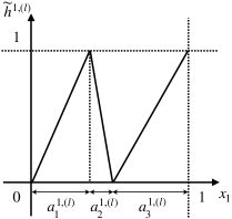
Figure 6: The graph of $\widetilde{h}^{1,(l)}$ for $p=3$

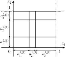
Figure 7: A decomposition of $[0,1]^{2}$ into rectangles ($2$-dim hypercuboids) by $\widetilde{h}^{(l)}$ for $n=2$, $p=3$

We remark that although the input space of $\widetilde{h}^{j,(l)}$ is $\mathbb{R}^{n}$, this map depends only on $j$-th entry of $\bm{x}$. Hence, we can regard this as from $\mathbb{R}$ to $\mathbb{R}$. Moreover, this map $\widetilde{h}^{j,(l)}$ divides the subinterval $[0,1]$ of $x_{j}$-axis into $p_{l}$ regions $(-\infty,0]$, $[0,a_{1}^{j,(l)}]$, $[a_{1}^{j,(l)},a_{1}^{j,(l)}+a_{2}^{j,(l)}]$, $\dots$, $[\sum_{i=1}^{p_{l}-1}a_{i}^{j,(l)},\infty)$ and the image of each regions by $\widetilde{h}^{j,(l)}$ is $[0,1]$. This construction makes a $p_{l}$-fold “folding”.

We define $\widetilde{h}^{(l)}\colon\mathbb{R}^{n}\to\mathbb{R}^{n}$ by $\widetilde{h}^{(l)}=(\widetilde{h}^{1,(l)},\dots,\widetilde{h}^{n,(l)})^{\top}$. By the construction, this map $\widetilde{h}^{(l)}$ can be realized as a ReLU neural network as

$$\mathbb{R}^{n}\to\mathbb{R}^{n_{l}}\to\mathbb{R}^{n};$$

$$\bm{x}\mapsto(h_{1}^{1,(l)}(\bm{x}),\dots,h^{n,(l)}_{p_{l}}(\bm{x}),0,\dots,0)^{\top}$$

$$\mapsto(\widetilde{h}^{1,(l)}(\bm{x}),\dots,\widetilde{h}^{n,(l)}(\bm{x}))^{\top}.$$

This map $\widetilde{h}^{(l)}$ divides $[0,1]^{n}\subset\mathbb{R}^{n}$ into $p_{l}^{n}$ $n$-dimensional hypercuboids. We remark that the volume of the $(i_{1},\dots,i_{n})$-th hypercuboid is $a^{1,(l)}_{i_{1}}a^{2,(l)}_{i_{2}}\cdots a_{i_{n}}^{n,(l)}$ as in Figure 7.

Then, the composition $\widetilde{h}^{(L-1)}\circ\cdots\circ\widetilde{h}^{(1)}$ defines the deep neural network of depth $L$, width $n_{0},n_{1},\dots,n_{L}$, and output $\mathbb{R}^{n}$. This map sends $[0,1]^{n}\in\mathbb{R}^{n}$ to $[0,1]^{n}\subset\mathbb{R}^{n}$ and divides $[0,1]^{n}$ into the $(p_{1}p_{2}\cdots p_{L-1})^{n}$ $n$-dimensional hypercubes with linear regions as in Figure 8. Then, the volume of $(\overline{i}_{1},\overline{i}_{2},\dots,\overline{i}_{n})$-th hypercube is

$$\left(a_{i_{1,L-1}}^{1,(L-1)}\cdots a_{i_{11}}^{1,(1)}\right) \cdot\left(a_{i_{2,L-1}}^{2,(L-1)}\cdots a_{i_{21}}^{2,(1)}\right)\cdot$$

$$\cdots\cdot\left(a_{i_{n,L-1}}^{n,(L-1)}\cdots a_{i_{n1}}^{n,(1)}\right),$$

where $\overline{i}_{k}=(i_{k1},\dots,i_{k,L-1})\in\prod_{l=1}^{L-1}\{1,\dots,p_{l}\}$.

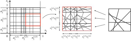
Figure 8: A grid decomposition of $[0,1]^{2}$ into rectangles by $\widetilde{h}^{(2)}\circ\widetilde{h}^{(1)}$ for $n=2,p_{1}=p_{2}=3$ and an image of copies of hyperplane arrangement in $[0,1]^{2}$ by $F$ into the rectangles

In particular, by perturbing weights if necessary, we may assume that any hypercuboids have different volumes.

Next, we choose a map $F\colon\mathbb{R}^{n}\to\mathbb{R}^{n_{L}}$ which gives a hyperplane arrangement whose chambers have different volumes introduced in Section 3.2 and by scaling, we assume that all the intersections of hyperplanes are in the interior of the hypercube $[0,1]^{n}\subset\mathbb{R}^{n}$. Finally, we take the composition $\widetilde{h}^{(L-1)}\circ\cdots\circ\widetilde{h}^{(1)}$ with $F$. Then, the hyperplanes arrangement in $[0,1]^{n}$ defined by $F$ is copied into each hypercuboids as in Figure 8. If we need, by perturbing weights again, we may assume that any linear region has different volume. This implies that the measure of complexity $c^{\sim}(F\circ\widetilde{h}^{(L-1)}\circ\cdots\circ\widetilde{h}^{(1)})$ coincides with the maximum of the number of linear regions. In particular, this is equal to

$$\prod_{i=1}^{L-1}\left(\left\lfloor\frac{n_{i}}{n}\right\rfloor\right)^{n}\left(\sum_{k=0}^{n}{n_{L}\choose k}\right).$$

This shows the following:

Theorem 4.

The measure of complexity $c^{\sim}(\mathcal{H}_{[0,1]^{n}}^{\mathrm{full}}(n_{0},n_{1},\dots,n_{L},n_{L+1}))$ for the model of above defined ReLU deep neural networks is bounded from below by $\prod_{i=1}^{L-1}\left(\left\lfloor\frac{n_{i}}{n}\right\rfloor\right)^{n}\left(\sum_{k=0}^{n}{n_{L}\choose k}\right)$.

As a consequence of the arguments of Section 3.2 and this section, both of the complexities for fully connected models which appear there are same as maximum numbers of linear regions. Hence, by similar argument to Montúfar et al., (2014), the complexity of deeper models is exponentially larger than the shallow models. This also shows the benefit of depth for neural network.

4.2 A benefit of depth for deep set models

We here consider a permutation-invariant deep model, called deep set model introduced by Zaheer et al., (2017). This model is made by stacking some permutation equivariant maps and one invariant map. Thus, the obtained map is permutation-invariant. This model has some common features with the model of Montúfar et al., (2014). Indeed, the original model of Montúfar et al, except for the map from the last hidden layer to the output layer, is equivalent to the deep set model. We shall modify the model variant introduced in Section 4.1 to be a deep set model and show that deep set models also have a similar benefit of depth.

As mentioned above, the deep set model is defined by stacking permutation equivariant affine maps and one invariant map. More specifically, the ReLU deep neural network $f_{L+1}\circ\mathrm{ReLU}\ \!\circ f_{L}\circ\cdots\circ\mathrm{ReLU}\ \!\circ f_{1}$ for affine maps $f_{i}\colon(\mathbb{R}^{n})^{m_{i-1}}\to(\mathbb{R}^{n})^{m_{i}}$ is called a deep set model if $f_{1},\dots,f_{L}$ are permutation equivariant and $f_{L+1}\colon(\mathbb{R}^{n})^{m_{L}}\to\mathbb{R}^{m_{L+1}}$ is permutation-invariant. For $\underline{m}=(m_{1},m_{2},\dots,m_{L},m_{L+1})$, let $\mathcal{H}_{[0,1]^{n}}^{\text{inv}}(n,\underline{m})$ be the set of the restrictions to $[0,1]^{n}$ of the deep set models.

If we assume that the variant of model of Montúfar et al., (2014) which we introduced in Section 4.1 satisfies that $h^{1,(l)}_{k}=\cdots=h^{n,(l)}_{k}$ for any $k$ and any $l$, and that $F\colon(\mathbb{R}^{n})^{m_{L}}\to\mathbb{R}^{m_{L+1}}$ is permutation-invariant, then the obtained neural network $F\circ\widetilde{h}^{(L-1)}\circ\cdots\circ\widetilde{h}^{(1)}$ is in $\mathcal{H}_{[0,1]^{n}}^{\text{inv}}(n,\underline{m})$. In this case, $a_{k}^{1,(l)}=\cdots=a_{k}^{n,(l)}$ holds for any $k$ and $l$. We set $a_{k}^{(l)}$ to be this number. The obtained neural network providing the $(\prod_{i=1}^{L-1}p_{l})^{n}$ $n$-dimensional hypercuboids. However, the volume of $(\overline{i}_{1},\overline{i}_{2},\dots,\overline{i}_{n})$-th hypercuboid is

$$\left(a_{i_{1,L-1}}^{(L-1)}\cdots a_{i_{11}}^{(1)}\right)\cdot\left(a_{i_{2,L-1}}^{(L-1)}\cdots a_{i_{21}}^{(1)}\right)\cdots\left(a_{i_{n,L-1}}^{(L-1)}\cdots\cdot a_{i_{n1}}^{(1)}\right),$$

where $\overline{i}_{k}=(i_{k,1},\dots,i_{k,L-1})\in\prod_{l=1}^{L-1}\{1,\dots,p_{l}\}$. We regard the index set $\prod_{l=1}^{L-1}\{1,\dots,p_{l}\}$ as an ordered set by the lexicographic order $\leq$. Then, by perturbing the weights or biases if we need, we may assume that any hypercuboid in the set of hypercuboids whose index $(\overline{i}_{1},\overline{i}_{2},\dots,\overline{i}_{n})$ satisfies $\overline{i}_{1}<\overline{i}_{2}<\dots<\overline{i}_{n}$ have different volumes, and the number of such hypercuboids is ${p_{1}\cdots p_{L-1}\choose n}$. We choose the affine map from $\mathbb{R}^{n}$ to output layer $(\mathbb{R}^{n})^{m_{L}}$ to be the one which achieves the measure of complexity of $\mathcal{H}_{[0,1]^{n}}^{\text{inv}}(n,nm_{L},m_{L+1})$ as in Section 3.3. Hence, the measure of complexity of $\mathcal{H}^{\text{inv}}(n,\underline{m})$ is bounded from below by $C\cdot(m_{1}\cdots m_{L})^{n}n^{n}/n!$ for a positive constant $C$. In particular, the following holds:

Theorem 5.

The following holds: $c^{\sim}(\mathcal{H}_{[0,1]^{n}}^{\mathrm{inv}}(n,\underline{m}))=\Omega((m_{1}\cdots m_{L})^{n}(n^{n}/n!))=\Omega((m_{1}\cdots m_{L}e)^{n}/\sqrt{n})$.

We compare this with the shallow invariant model having same number of hidden units. Then, the width of the hidden layer of the shallow model is equal to $n\sum_{i=1}^{L}m_{i}$. By the argument in Section 2.2, the measure of complexity is $\Theta((\sum_{i=1}^{L}m_{i})^{n}\cdot e^{n}/\sqrt{n})$. This yields that for the deep set model, deeper models can obtain exponentially more complexity than shallow models in our measure.

5 Conclusion

In this paper, we defined a new measure of complexity of ReLU neural networks, which is closer to expressive power than the number of linear regions. Specifically, we considered fully connected and Permutation-invariant models as examples, which are indistinguishable from the conventional measure of linear regions but have different expressive power. The new complexity is introduced as the number of equivalence classes that identify linear regions and linear functions on them with those transferred by a Euclidean transformation. Considering that, we have shown that the values of the measure for the two networks above are actually different. In this sense, the proposed measure of complexity can be considered to represent the expressive power of the function more closely. We also proved that the value of the proposed measure increases exponentially for deeper networks by refining the model of Montúfar et al., (2014) for both the fully connected model and the deep set model.

Acknowledgments

The authors would like to thank the anonymous reviewers for their suggestions and helpful comments. This work was supported in part by the Grant for Basic Science Research Projects from The Sumitomo Foundation (No.200484) and the JSPS Grant-in-Aid for Scientific Research C (20K03743).

Appendix A Illustrations and examples

A.1 Fully connected shallow model

In this section, we illustrate linear region calculations for simple examples in the plane.

In the two-dimensional plane, ”general position” means that two lines always intersect and three lines never are concurrent. Let us see an example in the case $n_{0}=2$, $n_{1}=4$, i.e., four lines in the plan.

$$\begin{cases}x-y+1=0&\ :\ H_{1}\\ x-y-1=0&\ :\ H_{2}\\ x+y-2=0&\ :\ H_{3}\\ x=\frac{1}{2}&\ :\ H_{4}.\end{cases}$$ (A.1)

This arrangement is not in general position because $H_{1}$ and $H_{2}$ are parallel or $H_{1}$, $H_{3}$ and $H_{4}$ are concurrent. Its number of chambers is $9$ (Figure 10)

Let us modify $H_{2}$ to make the arrangement being general position. Now we have:

$$\begin{cases}x-y+1=0&\ :\ H_{1}\\ y=1&\ :\ H_{2}\\ x+y-2=0&\ :\ H_{3}\\ x=\frac{1}{2}&\ :\ H_{4}.\end{cases}$$ (A.2)

Now the number of chambers is $11=\sum_{i=0}^{n_{0}}{n_{1}\choose i}$. It is maximal for a 4-line arrangement in the real plane (Figure 10).

Figure 9: The line arrangement not in general position. The number of chambers is 9.

Figure 10: The line arrangement in general position. The number of chambers is 11 and is maximal

A.2 Permutation invariant shallow model

Let us consider an example of a permutation-invariant shallow model with $m=n=2$, i.e., this model also implements a function from $\mathbb{R}^{2}$ to $\mathbb{R}^{4}$. We have the two pairs of lines (Figure 11):

$$\begin{cases}2x+\frac{1}{2}y-3=0&\ :\ H_{11}\\ \frac{1}{2}x+2y-3=0&\ :\ H_{12}\\ -x+6y=0&\ :\ H_{21}\\ 6x-y=0&\ :\ H_{22}.\end{cases}$$

We also count 11 chambers.

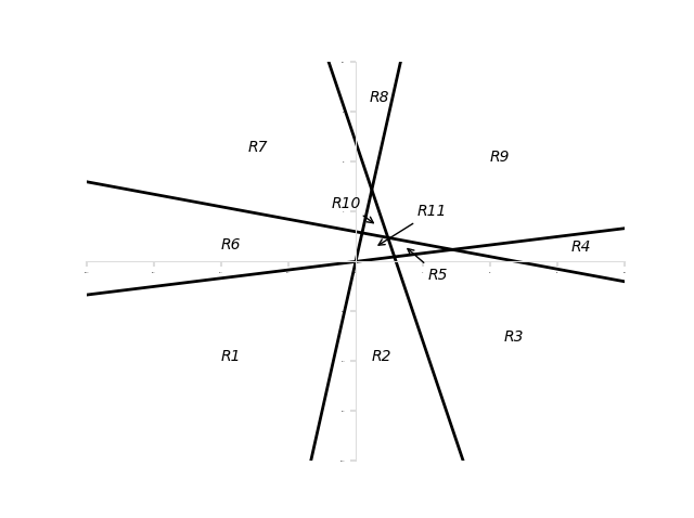
Figure 11: The 4 lines arrangement in the plane of a permutation invariant model. We count 11 linear regions.

A.3 Measure of complexity as the number of equivalent classes

Let us consider again the last invariant model example:

$$\begin{cases}2x+\frac{1}{2}y-3=0&\ :\ H_{11}\\ \frac{1}{2}x+2y-3=0&\ :\ H_{12}\\ -x+6y=0&\ :\ H_{21}\\ 6x-y=0&\ :\ H_{22}.\end{cases}$$ (A.3)

In this case, $S_{2}$ has a single element which is the permutation $\sigma=(1\ 2)$. Here, the action of $\sigma$ on $\mathbb{R}^{2}$ is exactly the action of the reflection symmetry through the line $x=y$. Then, the corresponding Euclidean transformation $\phi$ is $\phi=\begin{pmatrix}0&1\\ 1&0\end{pmatrix}$ and the underlying group is $\hat{\Phi}=\{I,\phi\}$

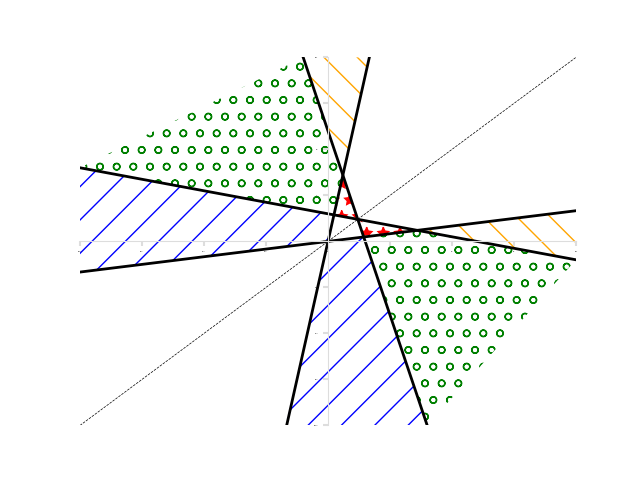
Figure 12: The dashed line is the line of equation $x=y$. We identify the equivalent regions with respect to the symmetry through the line $x=y$. The number of orbits is 7.

In Figure 12, we identify regions belonging to the same equivalent classes. In this case, a region is identified by its symmetry through the line $x=y$. Therefore, we count 7 equivalent classes of linear regions: {R1}, {R2,R6}, {R3,R7}, {R4,R8}, {R5,R10}, {R9}, {R11}.

Appendix B Proof of Proposition 1

In this section, we prove Proposition 1. To show this, we use the Deletion-Restriction theorem (Orlik and Terao,, 2013, Theorem 2.56 and Theorem 2.68).

Theorem 6 (Brylawsky, Zaslavsky).

For a hyperplane arrangement $\mathcal{A}$ in $\mathbb{R}^{n}$ and a fixed hyperplane $X\in\mathcal{A}$, let $(\mathcal{A},\mathcal{A}^{\prime},\mathcal{A}^{\prime\prime})$ be the triple defined as $\mathcal{A}^{\prime}=\mathcal{A}{\setminus}\{X\}$ and

$$\mathcal{A}^{\prime\prime}=\{H\cap X\mid H\in\mathcal{A}{\setminus}\{X\},H\cap X\neq\emptyset\}.$$

Then, the following holds:

$$|{\rm Ch}(\mathcal{A})|=|{\rm Ch}(\mathcal{A}^{\prime})|+|{\rm Ch}(\mathcal{A}^{\prime\prime})|.$$

By apply Theorem 6 to our hyperplane arrangement, we obtain a recurrence relation and calculate the number of linear regions for permutation invariant models.

Proof of Proposition 1.

Let $\mathcal{B}_{m,n}=\{H_{ij}\subset\mathbb{R}^{n}\mid i=1,\dots,m,\ j=1,\dots,n\}$ be the hyperplane arrangement defined by (2.7). We recall that hyperplanes of this arrangement $\mathcal{B}_{m,n}$ satisfy the following equations:

$$H_{i_{1},j}\cap H_{i_{2},j}\cap H_{i_{3},j}=\emptyset,$$ (B.1)

$$H_{i_{1},j_{1}}\cap H_{i_{1},j_{2}}\cap H_{i_{2},j_{1}}=H_{i_{1},j_{1}}\cap H_{i_{1},j_{2}}\cap H_{i_{2},j_{2}}=H_{i_{1},j_{1}}\cap H_{i_{2},j_{1}}\cap H_{i_{2},j_{2}}$$ (B.2)

for $i_{1},i_{2},i_{3}=1,\dots,m$ and $j,j_{1},j_{2}=1,\dots,n$.

We apply Theorem 6 to $\mathcal{B}_{m,n}$ and $H_{m,n}\in\mathcal{B}_{m,n}$. Then, we have

$$\mathcal{B}_{m,n}^{\prime} =\{H_{11},\dots,H_{1n},\dots,H_{m1},\dots,H_{m,n-1}\},$$

$$\mathcal{B}_{m,n}^{\prime\prime} =\{H_{11}\cap H_{m,n},\dots,H_{1n}\cap H_{m,n},\dots,H_{m1}\cap H_{m,n},\dots,H_{m,n-1}\cap H_{m,n}\}$$

and $|\mathcal{B}_{m,n}|=|\mathcal{B}_{m,n}^{\prime}|+|\mathcal{B}_{m,n}^{\prime\prime}|$ Here, because $H_{m,n}$ is a hyperplane bijective to $\mathbb{R}^{n-1}$, $H_{ij}\cap H_{m,n}$ can be regarded as a hyperplane in $H_{m,n}=\mathbb{R}^{n-1}$.

Next, we consider deletion and restriction for $\mathcal{B}_{m.n}^{\prime\prime}$ and $H_{m-1,n}\cap H_{m,n}$. Then, we have

$$(\mathcal{B}_{m,n}^{\prime\prime})^{\prime} =\left\{H_{1,1}\cap H_{m,n},\dots,H_{m-2,n}\cap H_{m,n},H_{m-1,1}\cap H_{m,n},\dots,H_{m-1,n-1}\cap H_{m,n},\atop H_{m,1}\cap H_{m,n},\dots,H_{m,n-1}\cap H_{m,n}\right\},$$

$$(\mathcal{B}_{m,n}^{\prime\prime})^{\prime\prime} =\left\{H_{1,1}\cap H_{m-1,n}\cap H_{m,n},\dots,H_{1,n}\cap H_{m-1,n}\cap H_{m,n},\dots,\atop H_{m,1}\cap H_{m-1,n}\cap H_{m,n},\dots,H_{m,n-1}\cap H_{m-1,n}\cap H_{m,n}\right\}.$$

Then, in the above $(\mathcal{B}_{m,n}^{\prime\prime})^{\prime\prime}$, by the relation (B.3), we have

$$H_{i,n}\cap H_{m-1,n}\cap H_{m,n}=\emptyset$$

for any $i=1,\dots,m-2$. Hence, any hyperplane of the form $H_{i,n}\cap H_{m-1,n}\cap H_{m,n}$ vanishes from $(\mathcal{B}_{m,n}^{\prime\prime})^{\prime\prime}$. Moreover, by the relation (B.4), for any $j=1,\dots,n-1$,

$$H_{m,j}\cap H_{m-1,n}\cap H_{m,n}=H_{m-1,j}\cap H_{m-1,n}\cap H_{m,n}$$

holds. By this relation, we can unify the hyperplanes of forms of $H_{m,j}\cap H_{m-1,n}\cap H_{m,n}$ and $H_{m-1,j}\cap H_{m-1,n}\cap H_{m,n}$. By these arguments, $(\mathcal{B}_{m,n}^{\prime\prime})^{\prime\prime}$ can be written by

$$(\mathcal{B}_{m,n}^{\prime\prime})^{\prime\prime}=\{H_{i,j}\cap H_{m-1,n}\cap H_{m,n}\subset\mathbb{R}^{n-2}\mid i=1,\dots,m-1,\ j=1,\dots,n-1\}.$$

Once, we set $\overline{H}_{i,j}=H_{i,j}\cap H_{m-1,n}\cap H_{m,n}\in(\mathcal{B}_{m,n}^{\prime\prime})^{\prime\prime}$. Then, it is easy to show that the obtained arrangement $(\mathcal{B}^{\prime\prime})^{\prime\prime}=\{\overline{H}_{i,j}\subset\mathbb{R}^{n-2}\mid i=1,\dots,m-1,j=1,\dots,n-1\}$ satisfies the following relations:

$$\overline{H}_{i_{1},j}\cap\overline{H}_{i_{2},j}\cap\overline{H}_{i_{3},j}=\emptyset,$$

$$\overline{H}_{i_{1},j_{1}}\cap\overline{H}_{i_{1},j_{2}}\cap\overline{H}_{i_{2},j_{1}}=\overline{H}_{i_{1},j_{1}}\cap\overline{H}_{i_{1},j_{2}}\cap\overline{H}_{i_{2},j_{2}}=\overline{H}_{i_{1},j_{1}}\cap\overline{H}_{i_{2},j_{1}}\cap\overline{H}_{i_{2},j_{2}}.$$

for $i_{1},i_{2},i_{3}=1,\dots,m-1$ and $j,j_{1},j_{2}=1,\dots,n-1$. This means that the hyperplane arrangement $(\mathcal{B}^{\prime\prime})^{\prime\prime}$ can be regarded as an arrangement “$\mathcal{B}_{m-1,n-1}$ in $\mathbb{R}^{n-2}$”. We will subsequently justify this argument more precisely.

Before we do it, we shall observe the deletion and restriction for $\mathcal{B}_{m,n}^{\prime}$ with $H_{m-1,n}\in\mathcal{B}_{m,n}^{\prime}$. Then, we have the following arrangements:

$$(\mathcal{B}_{m,n}^{\prime})^{\prime} =\{H_{1,1},\dots,H_{m-2,n},H_{m-1,1},\dots,H_{m-1,n-1},\dots,H_{m,1},\dots,H_{m,n-1}\},$$

$$(\mathcal{B}_{m,n}^{\prime})^{\prime\prime} =\left\{H_{11}\cap H_{m-1,n},\dots,H_{1,n}\cap H_{m-1,n},\dots,H_{m-1,1}\cap H_{m-1,n},\dots,\atop H_{m-1,n-1}\cap H_{m-1,n},H_{m,1}\cap H_{m-1,n},\dots,H_{m,n}\cap H_{m-1,n}\right\}.$$

Then, we remark that $(\mathcal{B}_{m,n}^{\prime})^{\prime\prime}$ is same as $(\mathcal{B}_{m,n}^{\prime\prime})^{\prime}$ if we exchange $H_{m-1,j}$ and $H_{m,j}$. By these relations, we have the following diagram:

To extract a recurrence relation from this diagram, we introduce another notation: Let

$$\mathcal{B}^{\ell}_{m,n}=\{X_{i,j}\subset\mathbb{R}^{\ell}\mid i=1,\dots,m,j=1,\dots,n\}$$

be a hyperplane arrangement in $\mathbb{R}^{\ell}$ satisfying the following relations:

$$X_{i_{1},j}\cap X_{i_{2},j}\cap X_{i_{3},j}=\emptyset,$$ (B.3)

$$X_{i_{1},j_{1}}\cap X_{i_{1},j_{2}}\cap X_{i_{2},j_{1}}=X_{i_{1},j_{1}}\cap X_{i_{1},j_{2}}\cap X_{i_{2},j_{2}}=X_{i_{1},j_{1}}\cap X_{i_{2},j_{1}}\cap X_{i_{2},j_{2}}$$ (B.4)

for $i_{1},i_{2},i_{3}=1,\dots,m$ and $j,j_{1},j_{2}=1,\dots,n$. Then, by the above arguments and a simple consideration, we have the following diagram:

$$\begin{aligned} \lx@xy@svg{\hbox{\raise 0.0pt\hbox{\kern 16.11745pt\hbox{\ignorespaces\ignorespaces\ignorespaces\hbox{\vtop{\kern 0.0pt\offinterlineskip\halign{\entry@#!@&&\entry@@#!@\cr&&\\&&\\&\\&\\\crcr}}}\ignorespaces{\hbox{\kern-11.45854pt\raise 0.0pt\hbox{\hbox{\kern 0.0pt\raise 0.0pt\hbox{\hbox{\kern 3.0pt\raise 0.0pt\hbox{$\textstyle{\mathcal{B}_{m,n}^{n}\ignorespaces\ignorespaces\ignorespaces\ignorespaces\ignorespaces\ignorespaces\ignorespaces\ignorespaces}$}}}}}}}\ignorespaces\ignorespaces\ignorespaces\ignorespaces{}{\hbox{\lx@xy@droprule}}\ignorespaces\ignorespaces\ignorespaces{\hbox{\kern 41.81221pt\raise 6.2111pt\hbox{{}\hbox{\kern 0.0pt\raise 0.0pt\hbox{\hbox{\kern 3.0pt\hbox{\hbox{\kern 0.0pt\raise-1.57222pt\hbox{$\scriptstyle{\cap X_{m,n}}$}}}\kern 3.0pt}}}}}}\ignorespaces{\hbox{\kern 90.77635pt\raise 0.0pt\hbox{\hbox{\kern 0.0pt\raise 0.0pt\hbox{\lx@xy@tip{1}\lx@xy@tip{-1}}}}}}{\hbox{\lx@xy@droprule}}{\hbox{\lx@xy@droprule}}\ignorespaces\ignorespaces\ignorespaces\ignorespaces{}{\hbox{\lx@xy@droprule}}\ignorespaces\ignorespaces\ignorespaces{\hbox{\kern 0.0pt\raise-18.97444pt\hbox{{}\hbox{\kern 0.0pt\raise 0.0pt\hbox{\hbox{\kern 3.0pt\hbox{\hbox{\kern 0.0pt\raise-1.57222pt\hbox{$\scriptstyle{{\setminus}X_{m,n}}$}}}\kern 3.0pt}}}}}}\ignorespaces{\hbox{\kern 0.0pt\raise-25.89333pt\hbox{\hbox{\kern 0.0pt\raise 0.0pt\hbox{\lx@xy@tip{1}\lx@xy@tip{-1}}}}}}{\hbox{\lx@xy@droprule}}{\hbox{\lx@xy@droprule}}{\hbox{\kern 90.77635pt\raise 0.0pt\hbox{\hbox{\kern 0.0pt\raise 0.0pt\hbox{\hbox{\kern 3.0pt\raise 0.0pt\hbox{$\textstyle{(\mathcal{B}_{m,n}^{n})^{\prime\prime}\ignorespaces\ignorespaces\ignorespaces\ignorespaces\ignorespaces\ignorespaces\ignorespaces\ignorespaces}$}}}}}}}\ignorespaces\ignorespaces\ignorespaces\ignorespaces{}{\hbox{\lx@xy@droprule}}\ignorespaces\ignorespaces\ignorespaces{\hbox{\kern 136.0713pt\raise 6.65833pt\hbox{{}\hbox{\kern 0.0pt\raise 0.0pt\hbox{\hbox{\kern 3.0pt\hbox{\hbox{\kern 0.0pt\raise-1.59167pt\hbox{$\scriptstyle{\cap(X_{m-1,n}\cap X_{m,n})}$}}}\kern 3.0pt}}}}}}\ignorespaces{\hbox{\kern 199.21013pt\raise 0.0pt\hbox{\hbox{\kern 0.0pt\raise 0.0pt\hbox{\lx@xy@tip{1}\lx@xy@tip{-1}}}}}}{\hbox{\lx@xy@droprule}}{\hbox{\lx@xy@droprule}}\ignorespaces\ignorespaces\ignorespaces\ignorespaces{}{\hbox{\lx@xy@droprule}}\ignorespaces\ignorespaces\ignorespaces{\hbox{\kern 107.66379pt\raise-18.97444pt\hbox{{}\hbox{\kern 0.0pt\raise 0.0pt\hbox{\hbox{\kern 3.0pt\hbox{\hbox{\kern 0.0pt\raise-1.59167pt\hbox{$\scriptstyle{{\setminus}(X_{m-1,n}\cap X_{m,n})}$}}}\kern 3.0pt}}}}}}\ignorespaces{\hbox{\kern 107.66379pt\raise-25.89333pt\hbox{\hbox{\kern 0.0pt\raise 0.0pt\hbox{\lx@xy@tip{1}\lx@xy@tip{-1}}}}}}{\hbox{\lx@xy@droprule}}{\hbox{\lx@xy@droprule}}{\hbox{\kern 199.21013pt\raise 0.0pt\hbox{\hbox{\kern 0.0pt\raise 0.0pt\hbox{\hbox{\kern 3.0pt\raise 0.0pt\hbox{$\textstyle{\mathcal{B}_{m-1,n-1}^{n-2}}$}}}}}}}{\hbox{\kern-16.11745pt\raise-37.94888pt\hbox{\hbox{\kern 0.0pt\raise 0.0pt\hbox{\hbox{\kern 3.0pt\raise 0.0pt\hbox{$\textstyle{(\mathcal{B}_{m,n}^{n})^{\prime}\ignorespaces\ignorespaces\ignorespaces\ignorespaces\ignorespaces\ignorespaces\ignorespaces\ignorespaces}$}}}}}}}\ignorespaces\ignorespaces\ignorespaces\ignorespaces{}{\hbox{\lx@xy@droprule}}\ignorespaces\ignorespaces\ignorespaces{\hbox{\kern 40.14555pt\raise-31.5239pt\hbox{{}\hbox{\kern 0.0pt\raise 0.0pt\hbox{\hbox{\kern 3.0pt\hbox{\hbox{\kern 0.0pt\raise-1.35834pt\hbox{$\scriptstyle{\cap X_{m-1,n}}$}}}\kern 3.0pt}}}}}}\ignorespaces{\hbox{\kern 86.11745pt\raise-37.94888pt\hbox{\hbox{\kern 0.0pt\raise 0.0pt\hbox{\lx@xy@tip{1}\lx@xy@tip{-1}}}}}}{\hbox{\lx@xy@droprule}}{\hbox{\lx@xy@droprule}}\ignorespaces\ignorespaces\ignorespaces\ignorespaces{}{\hbox{\lx@xy@droprule}}\ignorespaces\ignorespaces\ignorespaces{\hbox{\kern 0.0pt\raise-56.1861pt\hbox{{}\hbox{\kern 0.0pt\raise 0.0pt\hbox{\hbox{\kern 3.0pt\hbox{\hbox{\kern 0.0pt\raise-1.35834pt\hbox{$\scriptstyle{{\setminus}X_{m-1,n}}$}}}\kern 3.0pt}}}}}}\ignorespaces{\hbox{\kern 0.0pt\raise-64.42332pt\hbox{\hbox{\kern 0.0pt\raise 0.0pt\hbox{\lx@xy@tip{1}\lx@xy@tip{-1}}}}}}{\hbox{\lx@xy@droprule}}{\hbox{\lx@xy@droprule}}{\hbox{\kern 86.11745pt\raise-37.94888pt\hbox{\hbox{\kern 0.0pt\raise 0.0pt\hbox{\hbox{\kern 3.0pt\raise 0.0pt\hbox{$\textstyle{((\mathcal{B}_{m,n}^{n})^{\prime})^{\prime\prime}\ignorespaces\ignorespaces\ignorespaces\ignorespaces\ignorespaces\ignorespaces\ignorespaces\ignorespaces}$}}}}}}}\ignorespaces\ignorespaces\ignorespaces\ignorespaces{}{\hbox{\lx@xy@droprule}}\ignorespaces\ignorespaces\ignorespaces{\hbox{\kern 134.40463pt\raise-31.29056pt\hbox{{}\hbox{\kern 0.0pt\raise 0.0pt\hbox{\hbox{\kern 3.0pt\hbox{\hbox{\kern 0.0pt\raise-1.59167pt\hbox{$\scriptstyle{\cap(X_{m-2,n}\cap X_{m-1,n})}$}}}\kern 3.0pt}}}}}}\ignorespaces{\hbox{\kern 199.21013pt\raise-37.94888pt\hbox{\hbox{\kern 0.0pt\raise 0.0pt\hbox{\lx@xy@tip{1}\lx@xy@tip{-1}}}}}}{\hbox{\lx@xy@droprule}}{\hbox{\lx@xy@droprule}}\ignorespaces\ignorespaces\ignorespaces\ignorespaces{}{\hbox{\lx@xy@droprule}}\ignorespaces\ignorespaces\ignorespaces{\hbox{\kern 107.66379pt\raise-56.1861pt\hbox{{}\hbox{\kern 0.0pt\raise 0.0pt\hbox{\hbox{\kern 3.0pt\hbox{\hbox{\kern 0.0pt\raise-1.59167pt\hbox{$\scriptstyle{{\setminus}(X_{m-2,n}\cap X_{m-1,n})}$}}}\kern 3.0pt}}}}}}\ignorespaces{\hbox{\kern 107.66379pt\raise-64.42332pt\hbox{\hbox{\kern 0.0pt\raise 0.0pt\hbox{\lx@xy@tip{1}\lx@xy@tip{-1}}}}}}{\hbox{\lx@xy@droprule}}{\hbox{\lx@xy@droprule}}{\hbox{\kern 199.21013pt\raise-37.94888pt\hbox{\hbox{\kern 0.0pt\raise 0.0pt\hbox{\hbox{\kern 3.0pt\raise 0.0pt\hbox{$\textstyle{\mathcal{B}_{m-1,n-1}^{n-2}}$}}}}}}}{\hbox{\kern-6.75pt\raise-74.42332pt\hbox{\hbox{\kern 0.0pt\raise 0.0pt\hbox{\hbox{\kern 3.0pt\raise 0.0pt\hbox{$\textstyle{\vdots\ignorespaces\ignorespaces\ignorespaces\ignorespaces}$}}}}}}}\ignorespaces\ignorespaces\ignorespaces\ignorespaces{}{\hbox{\lx@xy@droprule}}\ignorespaces\ignorespaces\ignorespaces{\hbox{\kern 0.0pt\raise-92.55609pt\hbox{{}\hbox{\kern 0.0pt\raise 0.0pt\hbox{\hbox{\kern 3.0pt\hbox{\hbox{\kern 0.0pt\raise-1.35834pt\hbox{$\scriptstyle{{\setminus}X_{2,n}}$}}}\kern 3.0pt}}}}}}\ignorespaces{\hbox{\kern 0.0pt\raise-100.85555pt\hbox{\hbox{\kern 0.0pt\raise 0.0pt\hbox{\lx@xy@tip{1}\lx@xy@tip{-1}}}}}}{\hbox{\lx@xy@droprule}}{\hbox{\lx@xy@droprule}}{\hbox{\kern 100.91379pt\raise-74.42332pt\hbox{\hbox{\kern 0.0pt\raise 0.0pt\hbox{\hbox{\kern 3.0pt\raise 0.0pt\hbox{$\textstyle{\vdots\ignorespaces\ignorespaces\ignorespaces\ignorespaces}$}}}}}}}\ignorespaces\ignorespaces\ignorespaces\ignorespaces{}{\hbox{\lx@xy@droprule}}\ignorespaces\ignorespaces\ignorespaces{\hbox{\kern 107.66379pt\raise-92.55609pt\hbox{{}\hbox{\kern 0.0pt\raise 0.0pt\hbox{\hbox{\kern 3.0pt\hbox{\hbox{\kern 0.0pt\raise-1.59167pt\hbox{$\scriptstyle{{\setminus}(X_{1,n}\cap X_{2,n})}$}}}\kern 3.0pt}}}}}}\ignorespaces{\hbox{\kern 107.66379pt\raise-99.0511pt\hbox{\hbox{\kern 0.0pt\raise 0.0pt\hbox{\lx@xy@tip{1}\lx@xy@tip{-1}}}}}}{\hbox{\lx@xy@droprule}}{\hbox{\lx@xy@droprule}}{\hbox{\kern-6.54167pt\raise-110.68886pt\hbox{\hbox{\kern 0.0pt\raise 0.0pt\hbox{\hbox{\kern 3.0pt\raise 0.0pt\hbox{$\textstyle{\mathcal{B}\ignorespaces\ignorespaces\ignorespaces\ignorespaces\ignorespaces\ignorespaces\ignorespaces\ignorespaces}$}}}}}}}\ignorespaces\ignorespaces\ignorespaces\ignorespaces{}{\hbox{\lx@xy@droprule}}\ignorespaces\ignorespaces\ignorespaces{\hbox{\kern 42.56824pt\raise-104.26387pt\hbox{{}\hbox{\kern 0.0pt\raise 0.0pt\hbox{\hbox{\kern 3.0pt\hbox{\hbox{\kern 0.0pt\raise-1.35834pt\hbox{$\scriptstyle{\cap X_{1,n}}$}}}\kern 3.0pt}}}}}}\ignorespaces{\hbox{\kern 93.87192pt\raise-110.68886pt\hbox{\hbox{\kern 0.0pt\raise 0.0pt\hbox{\lx@xy@tip{1}\lx@xy@tip{-1}}}}}}{\hbox{\lx@xy@droprule}}{\hbox{\lx@xy@droprule}}\ignorespaces\ignorespaces\ignorespaces\ignorespaces{}{\hbox{\lx@xy@droprule}}\ignorespaces\ignorespaces\ignorespaces{\hbox{\kern 0.0pt\raise-129.30467pt\hbox{{}\hbox{\kern 0.0pt\raise 0.0pt\hbox{\hbox{\kern 3.0pt\hbox{\hbox{\kern 0.0pt\raise-1.35834pt\hbox{$\scriptstyle{{\setminus}X_{1,n}}$}}}\kern 3.0pt}}}}}}\ignorespaces{\hbox{\kern 0.0pt\raise-136.88162pt\hbox{\hbox{\kern 0.0pt\raise 0.0pt\hbox{\lx@xy@tip{1}\lx@xy@tip{-1}}}}}}{\hbox{\lx@xy@droprule}}{\hbox{\lx@xy@droprule}}{\hbox{\kern 93.87192pt\raise-110.68886pt\hbox{\hbox{\kern 0.0pt\raise 0.0pt\hbox{\hbox{\kern 3.0pt\raise 0.0pt\hbox{$\textstyle{\mathcal{B}_{m,n-1}^{n-1}}$}}}}}}}{\hbox{\kern-13.79187pt\raise-147.92049pt\hbox{\hbox{\kern 0.0pt\raise 0.0pt\hbox{\hbox{\kern 3.0pt\raise 0.0pt\hbox{$\textstyle{\mathcal{B}_{m,n-1}^{n}}$}}}}}}}\ignorespaces}}}}\ignorespaces\end{aligned} \textstyle{\mathcal{B}_{m,n}^{n}\ignorespaces\ignorespaces\ignorespaces\ignorespaces\ignorespaces\ignorespaces\ignorespaces\ignorespaces} \scriptstyle{\cap X_{m,n}} \scriptstyle{{\setminus}X_{m,n}} \textstyle{(\mathcal{B}_{m,n}^{n})^{\prime\prime}\ignorespaces\ignorespaces\ignorespaces\ignorespaces\ignorespaces\ignorespaces\ignorespaces\ignorespaces} \scriptstyle{\cap(X_{m-1,n}\cap X_{m,n})} \scriptstyle{{\setminus}(X_{m-1,n}\cap X_{m,n})} \textstyle{\mathcal{B}_{m-1,n-1}^{n-2}} \textstyle{(\mathcal{B}_{m,n}^{n})^{\prime}\ignorespaces\ignorespaces\ignorespaces\ignorespaces\ignorespaces\ignorespaces\ignorespaces\ignorespaces} \scriptstyle{\cap X_{m-1,n}} \scriptstyle{{\setminus}X_{m-1,n}} \textstyle{((\mathcal{B}_{m,n}^{n})^{\prime})^{\prime\prime}\ignorespaces\ignorespaces\ignorespaces\ignorespaces\ignorespaces\ignorespaces\ignorespaces\ignorespaces} \scriptstyle{\cap(X_{m-2,n}\cap X_{m-1,n})} \scriptstyle{{\setminus}(X_{m-2,n}\cap X_{m-1,n})} \textstyle{\mathcal{B}_{m-1,n-1}^{n-2}} \textstyle{\vdots\ignorespaces\ignorespaces\ignorespaces\ignorespaces} \scriptstyle{{\setminus}X_{2,n}} \textstyle{\vdots\ignorespaces\ignorespaces\ignorespaces\ignorespaces} \scriptstyle{{\setminus}(X_{1,n}\cap X_{2,n})} \textstyle{\mathcal{B}\ignorespaces\ignorespaces\ignorespaces\ignorespaces\ignorespaces\ignorespaces\ignorespaces\ignorespaces} \scriptstyle{\cap X_{1,n}} \scriptstyle{{\setminus}X_{1,n}} \textstyle{\mathcal{B}_{m,n-1}^{n-1}} \textstyle{\mathcal{B}_{m,n-1}^{n}} \textstyle{\mathcal{B}_{m,n}^{n}\ignorespaces\ignorespaces\ignorespaces\ignorespaces\ignorespaces\ignorespaces\ignorespaces\ignorespaces} \scriptstyle{\cap X_{m,n}} \scriptstyle{{\setminus}X_{m,n}} \textstyle{(\mathcal{B}_{m,n}^{n})^{\prime\prime}\ignorespaces\ignorespaces\ignorespaces\ignorespaces\ignorespaces\ignorespaces\ignorespaces\ignorespaces} \scriptstyle{\cap(X_{m-1,n}\cap X_{m,n})} \scriptstyle{{\setminus}(X_{m-1,n}\cap X_{m,n})} \textstyle{\mathcal{B}_{m-1,n-1}^{n-2}} \textstyle{(\mathcal{B}_{m,n}^{n})^{\prime}\ignorespaces\ignorespaces\ignorespaces\ignorespaces\ignorespaces\ignorespaces\ignorespaces\ignorespaces} \scriptstyle{\cap X_{m-1,n}} \scriptstyle{{\setminus}X_{m-1,n}} \textstyle{((\mathcal{B}_{m,n}^{n})^{\prime})^{\prime\prime}\ignorespaces\ignorespaces\ignorespaces\ignorespaces\ignorespaces\ignorespaces\ignorespaces\ignorespaces} \scriptstyle{\cap(X_{m-2,n}\cap X_{m-1,n})} \scriptstyle{{\setminus}(X_{m-2,n}\cap X_{m-1,n})} \textstyle{\mathcal{B}_{m-1,n-1}^{n-2}} \textstyle{\vdots\ignorespaces\ignorespaces\ignorespaces\ignorespaces} \scriptstyle{{\setminus}X_{2,n}} \textstyle{\vdots\ignorespaces\ignorespaces\ignorespaces\ignorespaces} \scriptstyle{{\setminus}(X_{1,n}\cap X_{2,n})} \textstyle{\mathcal{B}\ignorespaces\ignorespaces\ignorespaces\ignorespaces\ignorespaces\ignorespaces\ignorespaces\ignorespaces} \scriptstyle{\cap X_{1,n}} \scriptstyle{{\setminus}X_{1,n}} \textstyle{\mathcal{B}_{m,n-1}^{n-1}} \textstyle{\mathcal{B}_{m,n-1}^{n}}$$ (B.5)

Here, $\mathcal{B}$ is the hyperplane arrangement in $\mathbb{R}^{n}$ defined by

$$\mathcal{B}=\mathcal{B}_{m,n-1}^{n}\cup\{X_{1,n}\}.$$

Let $b_{m,n}^{\ell}=|{\rm Ch}(\mathcal{B}_{m,n}^{\ell})|$. Then, by Theorem 6 with the diagram (B.5), we have the recurrence relation

$$b_{m,n}^{n}=b_{m,n-1}^{n}+mb_{m,n-1}^{n-1}+\frac{m(m-1)}{2}b_{m-1,n-1}^{n-2}.$$

Moreover, by considering recursively, we can show that the following holds for $\ell,m,n\geq 1$:

$$b_{m,n}^{\ell}=b_{m,n-1}^{\ell}+mb_{m,n-1}^{\ell-1}+\frac{m(m-1)}{2}b_{m-1,n-1}^{\ell-2}.$$ (B.6)

Here, $b^{0}_{m,n}=b_{0,n}^{\ell}=b_{m,0}^{\ell}=1$ for any $\ell,m,n\geq 0$ and we set $b_{m,n}^{\ell}=0$ for $\ell<0$. Then, for example, by (B.6), we have $b^{1}_{m,n}=mn+1$ for any $m,n\geq 0$, $b^{\ell}_{m,1}=m^{2}/2+m/2+1$ for any $\ell\geq 2$ and $m$. In particular, $b_{m,n}^{\ell}$ is a polynomial with respect to $m$.

By this recurrence relation (B.6), we can represent $b_{m,n}^{n}$ as

$$b_{m,n}^{n}=\sum_{k=0}^{n/2}\sum_{\ell=0}^{n}d_{\ell,k}(m)b_{m-k,0}^{n-2k-\ell}=\sum_{k=0}^{n/2}\sum_{\ell=0}^{n}d_{\ell,k}(m),$$

where $d_{\ell,k}(m)$ is a non-negative integer. Here, the last equation follows from $b_{m-k,0}^{n-2k-\ell}=1$ for any $k,\ell,m$ such that $m-k\geq 0$ and $n-2k-\ell\geq 0$. Then, it is easy to show that $d_{\ell,k}(m)$ is obtained as a sum of multiples of $k$ times “$m(m-1)/2$”, $\ell$ times “$m$”, and $n-k-\ell$ times $1$. Here, these double quotation means that these vary in accordance with the order of the operations. Indeed, the iteration relation (B.6) can be represented as a higher-dimensional analogue of Pascal’s triangle as Figure 13.

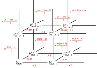
Figure 13: A higher dimensional analogue of Pascal’s triangle representing the iteration relation (B.6).

However, because we will calculate only the coefficient of leading term of $b_{m,n}^{n}$ as a polynomial of variable $m$, we may not take care of the orders. Then, the degree of $d_{\ell,k}(m)$ as a polynomial of variable $m$ is equal to $2k+\ell$. This means that the leading term of $b_{m,n}^{n}$ as a polynomial of variable $m$ is equal to the sum of terms $d_{\ell,k}(m)$ for $2k+\ell=n$. Moreover, by the fact $d_{\ell,k}(m)\geq 0$, we have

$$b_{m,n}^{n}=\sum_{k=0}^{n/2}\sum_{\ell=0}^{n}d_{\ell,k}(m)\geq\sum_{k=0}^{n/2}d_{n-2k,k}(m)=\text{(the leading term of }b_{m,n}^{n}\text{ as a polynomial of variable }m\text{)}.$$ (B.7)

We calculate a lower bound of the leading term. Then, the leading term of $d_{n-2k,k}(m)$ as a polynomial of $m$ can be written as

$$d_{n-2k,k}(m)={n\choose k,k,n-2k}\frac{1}{2^{k}}m^{n}+O(m^{n-1}),$$ (B.8)

where ${n\choose k_{1},\dots,k_{m}}$ for positive integers $k_{1},\dots,k_{m}$ such that $n=k_{1}+\cdots+k_{m}$ is the multinomial coefficient defined by

$${n\choose k_{1},\dots,k_{m}}=\frac{n!}{k_{1}!\cdots k_{m}!}={k_{1}\choose k_{1}}{k_{1}+k_{2}\choose k_{2}}\cdots{k_{1}+k_{2}+\cdots+k_{m}\choose k_{m}}.$$ (B.9)

Indeed, as mentioned before, $d_{n-2k,k}(m)$ is obtained as a sum of multiples of $k$ times of “$m(m-1)/2$”, $n-2k$ times of “$m$”, and $k$ times of $1$. Although the terms in the double quotations varies in accordance with the orders of the operations, the leading term is independent of the orders. Hence, the leading term of $d_{n-2k,k}(m)$ is the sum of multiples of $k$ times of $1/2$, $n-2k$ times of $1$, and $k$ times of $1$. The number of such multiples in the sum is same as ${n\choose k,k,n-2k}$. Hence, we have

$$d_{n-2k,k}(m)={n\choose k,k,n-2k}\frac{1}{2^{k}}m^{n}+O(m^{n-1}).$$

By the form of RHS of equation (B.9) and the estimate in (2.4), we have

$${n\choose k,k,n-2k} ={k\choose k}{2k\choose k}{n\choose n-2k}={2k\choose k}{n\choose n-2k}$$

$$\geq\frac{2^{kH(1/2)}}{\sqrt{8k(1-1/2)}}\frac{2^{nH((n-2k)/n)}}{\sqrt{8k(n-2k)(1-(n-2k)/n)}}$$

$$=\frac{2^{2k}2^{nH((n-2k)/n)}}{8k\sqrt{(n-2k)/n}}.$$ (B.10)

In the last inequality follows from $H(1/2)=1$.

We evaluate the coefficient of the leading term at $k=n/4$. Then, we have

$$d_{n/2,n/4}(m)\geq\frac{(2^{5/4})^{n}}{n\sqrt{2}}m^{n}+O(m^{n-1}).$$

In particular, the coefficient of leading term of $b_{m,n}^{n}$ is bounded from below by $(2^{5/4})^{n}/(n\sqrt{2})$. This concludes the proof. ∎

Appendix C Proof of Proposition 2

Proof of Proposition 2.

Let $\lambda\in\Lambda$, $\bm{x}\in D_{\lambda}$ and $\phi\in\Phi$. We assume that $\phi$ satisfies (1) $\phi(D_{\lambda})=D_{\lambda^{\prime}}$ and (2) $f_{\lambda}=f_{\lambda}\circ\phi|_{D_{\lambda}}$. Then, we have

$$f(\phi(\bm{x})) =f_{\lambda^{\prime}}(\phi(\bm{x}))=(f_{\lambda^{\prime}}\circ\phi|_{D_{\lambda}})(\bm{x})$$ (C.1)

$$=f_{\lambda}(\bm{x})=f(\bm{x}).$$ (C.2)

This equation holds for any $\bm{x}$ and any $\phi\in\Phi$. Because $\phi\in\Phi$ is a Euclidean transformation, $\phi$ is an isomorphism. In particular, the inverse of $\phi$ exists. As for any $\bm{y}\in\mathbb{R}^{n}$, there is a $\bm{x}$ such that $\bm{y}=\phi(\bm{x})$, by the equation (C.2), we have

$$f(\phi^{-1}(\bm{y}))=f(\bm{x})=f(\phi(\bm{x}))=f(\bm{y}).$$ (C.3)

Hence, $f$ is invariant by the action of $\phi^{-1}$ for any $\phi\in\Phi$. Now, let $\widehat{\Phi}$ be the subgroup of the group of Euclidean transformations generated by $\Phi$. This means that any element $\phi\in\widehat{\Phi}$ is a composition of finite elements of $\{\phi_{1},\dots,\phi_{t},\phi_{1}^{-1},\dots,\phi_{t}^{-1}\}$. Hence, by combining this fact and equations (C.2) and (C.3), $f$ is invariant by the action of the group $\widehat{\Phi}$. ∎

References

- Alex et al., (2012) Alex, K., Sutskever, Ilya, S., and Geoffrey E, H. (2012). Imagenet classification with deep convolutional neural networks. In Advances in neural information processing systems, pages 1097–1105.
- Arora et al., (2016) Arora, R., Basu, A., Mianjy, P., and Mukherjee, A. (2016). Understanding deep neural networks with rectified linear units. arXiv preprint arXiv:1611.01491.
- Ash, (1965) Ash, R. (1965). Information theory. Interscience Tracts in Pure and Applied Mathematics, No. 19. Interscience Publishers John Wiley & Sons, New York-London-Sydney.
- Bianchini and Scarselli, (2014) Bianchini, M. and Scarselli, F. (2014). On the complexity of neural network classifiers: A comparison between shallow and deep architectures. IEEE transactions on neural networks and learning systems, 25(8):1553–1565.
- Chatziafratis et al., (2020) Chatziafratis, V., Nagarajan, S. G., and Panageas, I. (2020). Better depth-width trade-offs for neural networks through the lens of dynamical systems. In International Conference on Machine Learning, pages 1469–1478. PMLR.
- Chatziafratis et al., (2019) Chatziafratis, V., Nagarajan, S. G., Panageas, I., and Wang, X. (2019). Depth-width trade-offs for relu networks via sharkovsky’s theorem. In International Conference on Learning Representations.
- Eldan and Shamir, (2016) Eldan, R. and Shamir, O. (2016). The power of depth for feedforward neural networks. In Conference on learning theory, pages 907–940.
- Goodfellow et al., (2013) Goodfellow, I. J., Bulatov, Y., Ibarz, J., Arnoud, S., and Shet, V. (2013). Multi-digit number recognition from street view imagery using deep convolutional neural networks. arXiv preprint arXiv:1312.6082.
- Hanin and Rolnick, (2019) Hanin, B. and Rolnick, D. (2019). Complexity of linear regions in deep networks. arXiv preprint arXiv:1901.09021.
- Kamiya et al., (2012) Kamiya, H., Takemura, A., and Terao, H. (2012). Arrangements stable under the coxeter groups. In Configuration spaces, pages 327–354. Springer.
- Maron et al., (2019) Maron, H., Fetaya, E., Segol, N., and Lipman, Y. (2019). On the universality of invariant networks. Proceedings of the 36th International Conference on Machine Learning, 97.
- Montúfar et al., (2014) Montúfar, G. F., Pascanu, R., Cho, K., and Bengio, Y. (2014). On the number of linear regions of deep neural networks. In Advances in neural information processing systems, pages 2924–2932.
- Orlik and Terao, (2013) Orlik, P. and Terao, H. (2013). Arrangements of hyperplanes, volume 300. Springer Science & Business Media.
- Pascanu et al., (2013) Pascanu, R., Montúfar, G., and Bengio, Y. (2013). On the number of response regions of deep feed forward networks with piece-wise linear activations. arXiv preprint arXiv:1312.6098.
- Raghu et al., (2017) Raghu, M., Poole, B., Kleinberg, J., Ganguli, S., and Dickstein, J. S. (2017). On the expressive power of deep neural networks. In Proceedings of the 34th International Conference on Machine Learning-Volume 70, pages 2847–2854. JMLR. org.
- Serra et al., (2018) Serra, T., Tjandraatmadja, C., and Ramalingam, S. (2018). Bounding and counting linear regions of deep neural networks. In International Conference on Machine Learning, pages 4558–4566.
- Silver et al., (2017) Silver, D., Schrittwieser, J., Simonyan, K., Antonoglou, I., Huang, A., Guez, A., Hubert, T., Baker, L., Lai, M., Bolton, A., et al. (2017). Mastering the game of go without human knowledge. Nature, 550(7676):354.
- Sonoda and Murata, (2017) Sonoda, S. and Murata, N. (2017). Neural network with unbounded activation functions is universal approximator. Applied and Computational Harmonic Analysis, 43(2):233–268.
- Telgarsky, (2016) Telgarsky, M. J. (2016). Benefits of depth in neural networks. Journal of Machine Learning Research, 49(June):1517–1539.
- Wan et al., (2013) Wan, L., Zeiler, M., Zhang, S., Le Cun, Y., and Fergus, R. (2013). Regularization of neural networks using dropconnect. In International conference on machine learning, pages 1058–1066.
- Yarotsky, (2017) Yarotsky, D. (2017). Error bounds for approximations with deep relu networks. Neural Networks, 94:103–114.
- Zaheer et al., (2017) Zaheer, M., Kottur, S., Ravanbakhsh, S., Poczos, B., Salakhutdinov, R. R., and Smola, A. J. (2017). Deep sets. In Advances in neural information processing systems, pages 3391–3401.