Vibrational heat-bath configuration interaction

Abstract

We introduce vibrational heat-bath configuration interaction (VHCI) as an accurate and efficient method for calculating vibrational eigenstates of anharmonic systems. Inspired by its origin in electronic structure theory, VHCI is a selected CI approach that uses a simple criterion to identify important basis states with a pre-sorted list of anharmonic force constants. Screened second-order perturbation theory and simple extrapolation techniques provide significant improvements to variational energy estimates. We benchmark VHCI on four molecules with 12 to 48 degrees of freedom and use anharmonic potential energy surfaces truncated at fourth and sixth order. For all molecules studied, VHCI produces vibrational spectra of tens or hundreds of states with sub-wavenumber accuracy at low computational cost.

I Introduction

Precise computational predictions of the vibrational structure of molecules and solids requires the inclusion of anharmonic effects, which correspond to interactions between harmonic normal modes. When treated quantum mechanically, this requires the accurate solution of the vibrational Schrödinger equation on a high-dimensional potential energy surface. Like in electronic structure theory, a hierarchy of wavefunction-based methods are commonly employed to avoid the exponential cost associated with an exact quantum solution; such methods include vibrational self-consistent field theory [1, 2, 3, 4] vibrational perturbation theory[5, 6, 7], vibrational coupled-cluster theory [8, 9, 10], and vibrational configuration interaction (VCI)[11, 12, 13]. These methods rely on the accuracy of the harmonic approximation and alternative methods have recently been developed to achieve quantitative accuracy for strongly anharmonic vibrations. Such methods include the nonproduct quadrature approach[14], reduced rank block power method (RRBPM), which uses a tensor factorization of the vibrational wavefunction [15], and adaptive VCI (A-VCI), which accelerates the VCI process using nested basis functions [16].

For strongly correlated electronic systems, the past two decades have seen the development of powerful computational methods that could be brought to bear on strongly anharmonic vibrational systems. For example, a vibrational density matrix renormalization group approach was recently developed and applied to systems with up to sixteen atoms [17]. In this work, we are primarily interested in selected configuration interaction [18, 19, 20], which began in the 1970s with CI by perturbatively selecting iteratively (CIPSI) [18] and has experienced renewed interest in the form of adaptive configuration interaction [21], adaptive sampling CI (ASCI) [22, 23], and heat-bath CI (HCI) [24, 25, 26, 27], among others. In CIPSI, many-body basis states are added to the variational CI space based on a first-order approximation of their wavefunction coefficients. Unlike CIPSI, which considers all states belonging to the first-order interacting space, ASCI only considers connections from the variational basis states that have sufficiently large wavefunction amplitudes. HCI uses a different selection criterion that allows it to exploit the fact that many Hamiltonian matrix elements are identical in magnitude; a presorting of these matrix elements (the two-electron repulsion integrals) enables fast and efficient identification of new basis states. In almost all selected CI calculations, once the variational space is suitably converged, a second-order perturbation theory (PT2) correction is added to the variational energy. Numerous recent studies have demonstrated their power: HCI was selected as the most accurate method among twenty for a study of transition metal atoms and their oxides [28], HCI was used to provide almost exact energies of the Gaussian-2 dataset [29], and both HCI and ASCI have been used in a recent comparative study of the ground-state energy of benzene [30].

A variety of selected CI approaches have been developed for vibrational problems [31, 32, 33, 34], including a vibrational CIPSI [35] and a recent vibrational ASCI (VASCI) [36]. Motivated by HCI’s strong performance and computational efficiency, in this work we present a vibrational HCI (VHCI). The differences between electronic and vibrational problems, especially their Hilbert spaces and Hamiltonian forms, necessitate a number of new developments in order for VHCI to enjoy the same advantages as electronic HCI; we describe these developments in Sec. II. In Sec. III, we present VHCI plus perturbation theory results for molecules containing between 12 and 48 degrees of freedom, calculating tens to hundreds of excited state energies. By comparing to other literature results, we demonstrate that VHCI is a highly accurate and efficient approach for large molecular systems with strong anharmonicity, typically achieving sub-wavenumber accuracy with modest computational resources.

II Theory

II.1 Vibrational heat-bath configuration interaction

Expressed in terms of mass-weighted normal mode coordinates $Q_{i}$ with frequencies $\omega_{i}$, the nuclear Hamiltonian is given by

$$H=\frac{1}{2}\sum_{i=1}^{D}\left[-\frac{\partial^{2}}{\partial Q_{i}^{2}}+\omega_{i}^{2}Q_{i}^{2}\right]+V_{\mathrm{an}}(Q_{1},Q_{2},\ldots,Q_{D}),$$ (1)

where $D=3N-6$ is the number of normal mode degrees of freedom and $V_{\mathrm{an}}$ is the anharmonic part of the electronic ground state potential energy surface (PES). We assume that the anharmonic part of the PES has a normal mode expansion

$$\begin{split}V_{\mathrm{an}}(\bm{Q})&=\sum_{i\leq j\leq k}V_{ijk}Q_{i}Q_{j}Q_{k}+\sum_{i\leq j\leq k\leq l}V_{ijkl}Q_{i}Q_{j}Q_{k}Q_{l}+\ldots\\ &=\sum_{i\leq j\leq k}W_{ijk}\bar{Q}_{i}\bar{Q}_{j}\bar{Q}_{k}+\sum_{i\leq j\leq k\leq l}W_{ijkl}\bar{Q}_{i}\bar{Q}_{j}\bar{Q}_{k}\bar{Q}_{l}+\ldots\\ \end{split}$$ (2)

where the anharmonic force constants are partial derivatives of the PES, e.g. $V_{ijk}=(\partial^{3}V_{\mathrm{an}}/\partial Q_{i}\partial Q_{j}\partial Q_{k})_{\bm{Q}=0}$. In the second line of Eq. (2), we define $\bar{Q}_{i}=(a_{i}^{\dagger}+a_{i})$ and

$$W_{ijk\ldots}=\frac{V_{ijk\ldots}}{\sqrt{2^{p}\omega_{i}\omega_{j}\omega_{k}\ldots}},$$ (3)

where $p$ is the order of the anharmonicity. In practice the anharmonic PES expansion is truncated, commonly at fourth or sixth order. In this work, we neglect the Coriolis rotational coupling, but such a term can be straightforwardly included.

In vibrational HCI, we choose to work in the basis of Hartree product states $|\bm{n}\rangle=|n_{1},n_{2},\ldots,n_{D}\rangle$ formed from the harmonic oscillator orbitals $\phi_{n_{i}}(Q_{i})=\langle Q_{i}|n_{i}\rangle$, leading to the wavefunction

$$\ket{\Psi}=\sum_{{\bm{n}}\in{\mathcal{V}}}c_{\bm{n}}\ket{{\bm{n}}}.$$ (4)

In VCI, the variational space ${\mathcal{V}}$ is commonly truncated by excitation level, for example by limiting the number of vibrational quanta per product state or per mode. However, this approach is not always efficient and may lead to a large Hilbert space with many product states that contribute minimally to the VCI solution. This issue of inefficient addition of states is addressed by selected VCI methods, which select states for inclusion in ${\mathcal{V}}$ by criteria other than excitation level as discussed in the Introduction, and here we focus on the HCI criterion.

We briefly recall that in the variational stage of HCI, basis state $\ket{{\bm{m}}}$ is added to ${\mathcal{V}}$ if $|H_{{\bm{m}}{\bm{n}}}c_{\bm{n}}|\geq\varepsilon_{1}$, where $\varepsilon_{1}$ is a user-defined convergence parameter. In electronic structure, the matrix elements $H_{{\bm{m}}{\bm{n}}}$ arising from double excitations depend only on the identity of the four orbitals involved. Therefore, many of the Hamiltonian matrix elements are identical in magnitude. This is not true in vibrational structure because the modes can have occupation numbers greater than one. For example, consider an anharmonic PES with cubic and quartic terms. The Hamiltonian matrix elements between product states $\ket{{\bm{m}}}$ and $\ket{{\bm{n}}}$ that differ in their occupancy by one quantum in mode $i$, by two quanta in modes $i$ and $j$ (including $i=j$), and so on, are given by

$$H_{{\bm{m}}{\bm{n}}}^{(i)} =\sum_{j}W_{ijj}\langle{\bm{m}}|\bar{Q}_{i}\bar{Q}_{j}^{2}|{\bm{n}}\rangle$$ (5a)

$$H_{{\bm{m}}{\bm{n}}}^{(i,j)} =\sum_{k}W_{ijkk}\langle{\bm{m}}|\bar{Q}_{i}\bar{Q}_{j}\bar{Q}_{k}^{2}|{\bm{n}}\rangle$$ (5b)

$$H_{{\bm{m}}{\bm{n}}}^{(i,j,k)} =W_{ijk}\langle{\bm{m}}|\bar{Q}_{i}\bar{Q}_{j}\bar{Q}_{k}|{\bm{n}}\rangle$$ (5c)

$$H_{{\bm{m}}{\bm{n}}}^{(i,j,k,l)} =W_{ijkl}\langle{\bm{m}}|\bar{Q}_{i}\bar{Q}_{j}\bar{Q}_{k}\bar{Q}_{l}|{\bm{n}}\rangle.$$ (5d)

The factors $\langle{\bm{m}}|\bar{Q}_{i}\ldots|{\bm{n}}\rangle$ that are not zero are products of terms of the form $\sqrt{n_{i}}$ and these factors are responsible for the differentiation of most matrix elements in the Hamiltonian, precluding an efficient evaluation of the usual HCI criterion. For example, if the product states $\ket{{\bm{m}}}$ and $\ket{{\bm{n}}}$ differ in the occupancy of three modes $(i,j,k)$, then

$$H_{{\bm{m}}{\bm{n}}}^{(i+,j+,k+)} =W_{ijk}\sqrt{m_{i}m_{j}m_{k}}$$ (6a)

$$H_{{\bm{m}}{\bm{n}}}^{(i+,j+,k-)} =W_{ijk}\sqrt{m_{i}m_{j}n_{k}}$$ (6b)

$$H_{{\bm{m}}{\bm{n}}}^{(i+,j-,k-)} =W_{ijk}\sqrt{m_{i}n_{j}n_{k}}$$ (6c)

and so on, where the notation indicates that the occupation of a given mode in $\ket{{\bm{m}}}$ is bigger or smaller than in $\ket{{\bm{n}}}$. Therefore, in addition to the identity of the modes with different occupations, the VCI matrix elements depend on (1) whether the occupations are bigger/smaller on the bra/ket side, and (2) the overall excitation level. However, because these latter factors $\langle{\bm{m}}|\bar{Q}_{i}\ldots|{\bm{n}}\rangle$ are products of terms of the form $\sqrt{n_{i}}$, they are of order unity (at least when the excitation level is reasonably low) and can be reasonably neglected for the purpose of estimating the magnitude of the Hamiltonian matrix element. Doing so leads to a significant reduction in the number of unique numbers to be considered.

Specifically, let us define $W_{i}=\sum_{j}(2+\delta_{ij})W_{ijj}$ and $W_{ij}=\sum_{k}(2+\delta_{jk}+\delta_{ij}\delta_{jk})W_{ijkk}$, which approximately account for single and double mode excitations. Then, given an approximate wavefunction of the form (4) expanded over some space ${\mathcal{V}}$, we propose to add state $\ket{{\bm{m}}}$ to the variational space if $\ket{{\bm{m}}}$ and $\ket{{\bm{n}}}$ differ in their occupancy by one quantum in mode $i$, by two quanta in modes $i$ and $j$ (including $i=j$), and so on, and

$$\left|W_{ijk\ldots}c_{\bm{n}}\right|\geq\varepsilon_{1}.$$ (7)

The above criterion can be implemented very efficiently by pre-sorting the matrix elements $W_{ijk\ldots}$, of which there are at most a polynomial number, e.g. $O(D^{4})$ for a quartic PES.

The ground-state VHCI algorithm is performed as follows:

1. Sort the list of $W_{ijk\ldots}$, largest to smallest.

2. Initialize the space ${\mathcal{V}}$ according to a small total number of quanta.

3. Build the Hamiltonian matrix in ${\mathcal{V}}$ and calculate its ground-state eigenvalue and eigenvector.

4. Add states to ${\mathcal{V}}$ via the criterion (7), as follows. For each state $\ket{{\bm{n}}}$, traverse the sorted list of $W_{ijk\ldots}$.

   1. If $|W_{i}c_{\bm{n}}|\geq{\varepsilon}_{1}$, add all states $\ket{{\bm{m}}}$ that are included in $Q_{i}\ket{{\bm{n}}}$.

   2. If $|W_{ij}c_{\bm{n}}|\geq{\varepsilon}_{1}$, add all states $\ket{{\bm{m}}}$ that are included in $Q_{i}Q_{j}\ket{{\bm{n}}}$.

   3. If $|W_{ijk\ldots}c_{\bm{n}}|\geq{\varepsilon}_{1}$, add all states $\ket{{\bm{m}}}$ that are included in $Q_{i}Q_{j}Q_{k}\ldots\ket{{\bm{n}}}$. At anharmonic order $p$, there are $O(2^{p})$ such states to add.

   4. If $|W_{ijk\ldots}c_{\bm{n}}|<{\varepsilon}_{1}$, break and go on to the next $\ket{{\bm{n}}}$.

   Return to step 3 until the calculation is converged.

A number of possible convergence criteria can be devised; here, following the original HCI paper [24], we consider the calculation converged when the total number of states added in step 4 is less than 1% of the current number of variational states. Importantly, most elements of $H_{{\bm{m}}{\bm{n}}}$ are zero due to the properties of harmonic oscillators; the states $\ket{{\bm{m}}}$ and $\ket{{\bm{n}}}$ can only differ by a few quanta, depending on the maximum anharmonic order of the PES. The same would not be true in the basis of product states obtained after a vibrational self-consistent field procedure [1, 2, 3, 4], which is why we intentionally work in the noninteracting normal mode basis.

Crucially, the presorting of scaled and/or summed anharmonic force constants $(W_{i},W_{ij},W_{ijk\ldots})$ combined with the criterion (7) means that most states $\ket{{\bm{m}}}$ are never even tested for addition. Just like in electronic structure theory, this construction is the key to the efficiency of VHCI. Unlike in electronic structure theory, the ground state of the vibrational Schrödinger equation, referred to here as the zero-point energy (ZPE), is rarely of interest by itself. Following Ref. 25, we can straightforwardly modify the above VHCI algorithm to allow the simultaneous calculation of many excited states. In step 3, we find all eigenstates of interest (typically the $N_{\mathrm{s}}$ lowest in energy). Then we perform the addition step 4 for each of those states, combining all of their added basis states $\ket{{\bm{m}}}$ in the updated ${\mathcal{V}}$. Clearly, this adds many more basis states at each iteration, but many of them are duplicates and so the overall variational space is observed to grow sublinearly with $N_{\mathrm{s}}$.

The above procedure can be applied to a PES expanded to arbitrary order in the normal mode coordinates. However, high-order anharmonic interactions with repeated mode indices will contribute to lower-order excitations beyond the single and double excitations described in Eqs. (5a) and (5b) for the case of a quartic PES. For example, a sixth-order PES will yield triple excitations due to cubic anharmonicity and fifth-order anharmonicity (when a mode index is repeated), and similarly quadruple excitations due to quartic and sixth-order anharmonicity. In this work, we only test one sixth-order PES in Sec. III.4; although we could define new effective force constants for the screening procedure, e.g. $W_{ijk}^{\prime}=W_{ijk}+\sum_{k}W_{ijkll}$, instead we make the approximation $\sum_{l}W_{ijkll}\approx\max_{l}W_{ijkll}$. In other words, we allow fifth-order anharmonicities to propose triple excitations, but only based on the magnitude of individual anharmonic force constants and not the sum of all such constants contributing to a given triple excitation. Our testing suggests that the error incurred is negligible.

II.2 Epstein-Nesbet perturbation theory

To the variational energy of each state $E_{\mathrm{var}}$ we add the second-order perturbation theory (PT2) correction

$$\Delta E_{2}\approx\sum_{\bm{m}}^{({\varepsilon}_{2})}\frac{\left(\sum_{\bm{n}}H_{{\bm{m}}{\bm{n}}}c_{\bm{n}}\right)^{2}}{E_{\mathrm{var}}-H_{{\bm{m}}{\bm{m}}}}.$$ (8)

In exact PT2, the summation over ${\bm{m}}$ includes all basis states that are connected to the variational space ${\mathcal{V}}$. For large variational spaces, this perturbative space is enormous and the cost of the PT2 correction is prohibitive. To address this, HCI uses the same screening procedure as in the variational stage to efficiently include only the most important perturbative states [24]. For VHCI, we again use criterion (7), with a cutoff $\varepsilon_{2}<\varepsilon_{1}$, to determine whether basis state $\ket{{\bm{m}}}$ should be included in the perturbative space. When $\varepsilon_{2}=0$, the PT2 calculation is exact within the first-order interacting space.

Throughout this work, we calculate the PT2 correction deterministically as described above, which ultimately limits the size of the systems that we can accurately study. In the future we will pursue the stochastic or semistochastic evaluation of Eq. (8), as is now common practice in HCI [26], in order to study the vibrational structure of even larger systems.

III Results

Table 1: The twenty lowest-energy states from a calculation of the first 70 eigenstates of acetonitrile, with excitation energies given relative to the ZPE. Mode assignments are given based on the character of the basis state with the largest absolute CI coefficient, using mode-numbering from Ref. 37 and showing multiple assignments when their weights differ by less than 0.1. VHCI results are shown for two different values of ${\varepsilon}_{1}$, which determines the number of variational basis states, $N_{\mathcal{V}}$, and shown with and without the PT2 correction to the energies (“Var” and “Full PT2”, respectively). We compare to exact reference values from A-VCI [16] and to VASCI with full PT2 correction and $N_{\mathcal{V}}$ comparable to our ${\varepsilon}_{1}=1.0$ cm^-1 case [36]. The maximum absolute error (Max. AE) and root mean squared error (RMSE) relative to A-VCI were calculated across all 70 states. All energies are in cm^-1.

Method:	${\varepsilon}_{1}=1.0$		${\varepsilon}_{1}=0.1$		VASCI[36]	A-VCI[16]
$N_{\mathrm{\mathcal{V}}}$:	29 900		125 038		30 038	2 488 511
	Var	Full PT2	Var	Full PT2	Full PT2	Var
ZPE	9837.43	9837.41	9837.41	9837.41	9837.41	9837.41
$\omega_{11}$	361.01	360.99	360.99	360.99	361.01	360.99
$\omega_{12}$	361.01	360.99	360.99	360.99	361.01	360.99
$\omega_{11}+\omega_{12}$	723.22	723.18	723.18	723.18	723.22	723.18
$2\omega_{11},~{}2\omega_{12}$	723.25	723.19	723.18	723.18	723.23	723.18
$2\omega_{11},~{}2\omega_{12}$	723.90	723.84	723.83	723.83	723.89	723.83
$\omega_{4}$	900.70	900.66	900.66	900.66	900.68	900.66
$\omega_{9}$	1034.18	1034.13	1034.13	1034.12	1034.14	1034.12
$\omega_{10}$	1034.19	1034.13	1034.13	1034.12	1034.14	1034.13
$\omega_{11}+2\omega_{12}$	1086.65	1086.56	1086.56	1086.55	1086.64	1086.55
$2\omega_{1}+\omega_{12}$	1086.66	1086.56	1086.56	1086.55	1086.64	1086.55
$3\omega_{11}$	1087.88	1087.79	1087.78	1087.78	1087.88	1087.77
$3\omega_{12}$	1087.88	1087.79	1087.78	1087.78	1087.88	1087.77
$\omega_{4}+\omega_{11}$	1259.89	1259.82	1259.81	1259.81	1259.86	1259.81
$\omega_{4}+\omega_{12}$	1259.94	1259.83	1259.82	1259.81	1259.86	1259.81
$\omega_{3}$	1389.10	1388.99	1388.98	1388.97	1388.99	1388.97
$\omega_{11}+\omega_{10},~{}\omega_{9}+\omega_{12}$	1394.86	1394.71	1394.69	1394.68	1394.76	1394.68
$\omega_{9}+\omega_{11},~{}\omega_{10}+\omega_{12}$	1394.89	1394.71	1394.70	1394.68	1394.79	1394.68
$\omega_{11}+\omega_{10},~{}\omega_{9}+\omega_{12}$	1395.08	1394.93	1394.91	1394.90	1395.00	1394.90
$\omega_{3}$	1397.83	1397.70	1397.69	1397.68	1397.77	1397.68
Max. AE(70):	0.61	0.14	0.05	0.01	0.50	–
RMSE(70):	0.34	0.05	0.03	0.00	0.20	–

III.1 Software and simulation details

All simulations besides those on naphthalene were performed on a 4-core (8-thread) Intel Core i7-6700 3.4 GHz desktop CPU using up to 16 GB of RAM. Naphthalene calculations were performed on a cluster with up to two 12-core Intel Xeon Gold 6126 2.6 GHz CPUs and using up to 768 GB of RAM.

Our code is based on the Ladder Operator Vibrational Configuration Interaction package [38] with extensive modifications. Our VHCI code is available on GitHub [39]. The Hamiltonian matrix is stored in a sparse format using the Eigen linear algebra library [40]. The eigenvalues and eigenvectors of interest are calculated with the Lanczos algorithm as implemented in the SPECTRA linear algebra library [41]. We verified our code by comparing to the literature and to results obtained with the PyVCI software package [34].

All VHCI calculations were initialized with a basis of all states containing up to two vibrational quanta in order to ensure that two-quantum overtones and combination bands, which account for many of the low-lying target states, are present from the first iteration. Our preliminary testing indicates that using a larger initial basis does not qualitatively improve the convergence of the results.

III.2 Acetonitrile: A standard benchmark

We first present results for acetonitrile, CH₃CN, a 6-atom, 12-dimensional system that has become one of the canonical benchmarks for new methods in vibrational structure theory [15, 42, 17, 43, 36]. We use the quartic PES described in Refs. 44, 15, for which normal mode frequencies were calculated using CCSD(T)/cc-pVTZ and higher-order force constants were calculated using B3LYP/cc-pVTZ. This PES was also used in highly accurate reference calculations [14, 37]. All PESs used in this study are available as input files on our GitHub repository [39].

We calculated the energies of the first 70 states of acetonitrile, of which the first 20 are reported in Table 1. Data for all 70 states can be found in the supplementary material. We compare our results to those obtained using A-VCI [37], which we consider to be numerically exact (similar to those obtained with the nonproduct quadrature approach [14]); for reference, the A-VCI results are obtained with approximately 2.5 million variational states. Mode assignments here and throughout indicate the character of the product state with the largest weight in the VCI eigenvector; for acetonitrile, we use the mode-numbering convention of Ref. 37. To quantitatively assess the accuracy of our results, we report the maximum absolute error and the root mean squared error of the lowest 70 states. In addition to the numerically exact A-VCI results, we also compare to results obtained recently using VASCI [36], which is a selected CI technique that is similar in spirit to VHCI.

We report results for variational VHCI (“Var”), as well as VHCI+PT2 without VHCI screening of the perturbative space (“Full PT2”); these results are given for two values of the variational energy cutoff ${\varepsilon}_{1}$ that controls the number of variational states $N_{\mathcal{V}}$. Using ${\varepsilon}_{1}=1$ cm^-1 results in a variational space with $N_{\mathcal{V}}=29\,900$ basis states, which enables comparison to the largest reported VASCI calculation, with $N_{\mathcal{V}}=30\,038$. We find that VHCI+PT2 achieves a maximum absolute error and a root mean squared error that is less than half that of VASCI, which is somewhat surprising because the CIPSI-style selection criterion used in VASCI is typically thought to more rigorously identify important states. However, the precise variational space generated by both VHCI and VASCI can be tuned by their parameters ($\varepsilon_{1}$ and the number of core/target states, respectively), so a direct comparison is not straightforward. In any event, the accuracy of VHCI is remarkable given the modest computational cost; for example, the ${\varepsilon}_{1}=1$ cm^-1 calculation reported here took less than 3 minutes for the variational stage and less than 30 minutes for the full PT2 correction (on an 8-core desktop CPU).

Table 2: The sixteen lowest-energy states from a calculation of the first 100 eigenstates of ethylene, with excitation energies given relative to the ZPE. Calculations were performed using fourth- and sixth-order truncations of the PES normal mode expansion. Both VHCI+PT2 calculations were converged with respect to variational and perturbative basis size. We compare to vDMRG[17] for both truncations and to VCI[34] with up to 8 quanta per product state for the sixth-order truncation. We also compare to a calculation from Ref. 45 which uses an untruncated version of the PES solved using VCI with a pruned basis set containing up to 13 quanta per product state. Assignments are given using the mode-numbering convention of Ref. 45. All energies are in cm^-1.

PES:	Fourth-order		Sixth-order			Untruncated
Method:	VHCI+Full PT2	vDMRG[17]	VHCI+PT2 (${\varepsilon}_{2}=0.01$)	vDMRG[17]	VCI (PyVCI)[46]	Pruned VCI[45]
	${\varepsilon}_{1}=0.75$		${\varepsilon}_{1}=0.5$		$N_{\mathrm{tot}}=8$	$N_{\mathrm{tot}}=13$
ZPE	11006.11	11006.19	11011.61	11016.15	11011.63	11014.91
$\omega_{10}$	808.61	809.03	819.99	831.17	820.11	822.42
$\omega_{8}$	914.87	915.29	926.33	933.47	926.45	934.29
$\omega_{7}$	927.87	928.31	941.65	948.26	941.78	949.51
$\omega_{4}$	1006.74	1007.13	1017.45	1018.26	1017.56	1024.94
$\omega_{6}$	1216.94	1217.17	1222.16	1227.05	1222.23	1224.96
$\omega_{3}$	1338.46	1338.87	1341.95	1343.46	1342.01	1342.96
$\omega_{12}$	1429.93	1430.47	1438.31	1441.52	1438.39	1441.11
$\omega_{2}$	1606.41	1622.11	1622.78	1629.04	–	1624.43
$2\omega_{10}$	1631.47	1625.56	1655.21	1682.18	–	1658.39
$\omega_{8}+\omega_{10}$	1718.27	1722.77	1748.05	1770.02	–	1757.70
$\omega_{7}+\omega_{10}$	1733.98	1729.53	1766.19	1786.99	–	1778.34
$\omega_{4}+\omega_{10}$	1809.39	1810.47	1837.68	1852.60	–	1848.61
$2\omega_{8}$	1821.71	1826.01	1858.36	1878.42	–	1873.73
$\omega_{7}+\omega_{8}$	1821.96	1827.96	1871.42	1886.16	–	1885.12
$2\omega_{7}$	1850.39	1852.23	1887.03	1906.02	–	1901.61

In Table 1, we also present results of a larger calculation with ${\varepsilon}_{1}=0.1$ cm^-1, resulting in $N_{\mathcal{V}}=125~{}038$. We obtain an extremely accurate spectrum even without the PT2 correction, with a maximum absolute error well below 0.1 cm^-1. This variational calculation took less than 30 minutes on the same 8-core desktop CPU. This larger calculation still benefits from minor corrections with PT2, which takes about three hours and produces a spectrum in which no value differs from the exact result by more than 0.01 cm^-1 across all 70 states. In summary, we have shown that VHCI can produce near-exact results for a 12-dimensional system with an extremely small computational effort.

III.3 Ethylene: Sixth-order potential

Next, we study ethylene, C₂H₄, which is the same size as acetonitrile (6 atoms, 12 dimensions), but here we use a more realistic ab initio potential energy surface and consider anharmonic expansions up to sixth order. Specifically, we use the PES of Ref. 45, which was calculated entirely using CCSD(T)/cc-pVQZ, and we use the PyPES software package [46] to convert from internal to cartesian normal mode coordinates and generate an anharmonic expansion up to sixth order. In contrast to the quartic PES of acetonitrile that contains 299 nonzero anharmonic force constants, this sixth-order PES for ethylene contains 2651 force constants, 2375 of which are fifth or sixth order. Here, we compare results and performance when the potential is truncated at fourth order and at sixth order. We calculated the first 100 states; results for the first sixteen states are shown in Table 2 and those for the additional 84 states can be found in the supplementary material.

Through testing, we confirmed that our VHCI+PT2 results are converged with ${\varepsilon}_{1}=0.75$ cm^-1 for the quartic case (with full PT2) and ${\varepsilon}_{1}=0.5$ cm^-1 for the sixth-order case (with ${\varepsilon}_{2}=0.01$ cm^-1), resulting in $N_{\mathcal{V}}=$ 153 935 and 161 338 basis states, respectively. In fact, it was not possible to go to larger variational spaces for the quartic case because of unphysical divergences in the truncated PES. Similar behavior of truncated PESs studied at high excitation levels has been observed before [45, 34, 47].

In Table 2, we also compare our results to those obtained with the vibrational density-matrix renormalization group (vDMRG) [17] using the same fourth- and sixth-order truncated PES. As discussed in the Introduction, DMRG and selected CI are similarly competitive methods in electronic structure theory. Surprisingly, we find that for both truncations, our energies are noticeably lower than the vDMRG results. For the quartic potential, our zero-point energy is 0.8 cm^-1 lower than the vDMRG result, while for the sixth-order potential it is 4.5 cm^-1 lower. Figure 1 shows the convergence of the ZPE as a function of the size of the variational space, $N_{\mathcal{V}}$. We see that VHCI (obtained with $N_{\mathrm{s}}=1$) converges smoothly and quickly; for the fourth-order potential it exceeds the accuracy of vDMRG with about 5000 basis states. We also show results obtained with our own VCI code, which includes basis states according to their total number of vibrational quanta. For both the fourth- and sixth-order potentials, VCI converges to the same ZPE as VHCI, although it requires significantly more basis states for comparable accuracy. The discrepancy with vDMRG may come from the latter using insufficient bond dimension, getting trapped in local minima during sweeps, or simply due to slight differences in the PES. As a check on the latter, we have also included in Table 2 the VCI excitation energies previously reported by the authors of the PyPES software package [34] from which the PES parameters were obtained. The results are in excellent agreement with our own VHCI+PT2 results, indicating that we are using the exact same PES as those authors.

In Fig. 1, we also plot the percent sparsity of the Hamiltonian matrix as function of number of variational basis states. We present the sparsity for VHCI (optimized for the ground state) and conventional VCI. For both the fourth-order and sixth-order potentials, VHCI produces a much sparser Hamiltonian matrix than VCI. These results indicate that VHCI is extremely effective at capturing the connectivity between important basis states (as demonstrated by the accurate ground-state energy) while also ignoring the connectivity to less important basis states (as demonstrated by the increased sparsity).

In the final column of Table 2, we also show results obtained in Ref. 45 using a pruned VCI basis with up to 13 vibrational quanta for the untruncated PES. In its current form, VHCI requires the truncated normal mode expansion (2) and thus comparison to the results obtained for an untruncated PES is important for assessing the future potential of VHCI. As can be seen, the agreement improves significantly when going from the fourth-order PES to the sixth-order PES. For low-lying states, the disagreement at fourth order is on the order of 10-20 cm^-1 and at sixth order is on the order of 5 cm^-1, indicating that the normal mode expansion is sensible and systematically improvable.

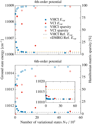
Figure 1: The variational ground-state energy of ethylene as a function of number of basis states $N_{\mathcal{V}}$. We compare the ground state energies of conventional VCI (solid red circles) and VHCI (solid blue squares) using a fourth-order (top) and sixth-order (bottom) truncation of the potential. VHCI calculations were performed by optimizing for the ground state ($N_{\mathrm{s}}=1$) and the VCI space was truncated by limiting the total number of quanta per product state. The blue dashed lines represent the converged VHCI ground-state energy, which we consider to be exact. The orange dashed lines are the vDMRG values from Ref. 17. We also present the sparsity of the Hamiltonian matrix (right axis) as a function of $N_{\mathcal{V}}$ for conventional VCI (open red circles) and VHCI (open blue squares).

III.4 Ethylene oxide: Convergence and extrapolation

Next, we study ethylene oxide, C₂H₄O, a molecule with 7 atoms and 15 normal mode degrees of freedom. Compared to the two previous molecules, the three additional degrees of freedom make numerically exact VCI calculations much more difficult. We use the quartic PES of Bégué et al.[48], with normal mode frequencies calculated at the CCSD(T)/cc-pVTZ level and anharmonic force constants calculated using B3LYP/6-31+G(d,p). We use the same version of the PES as Refs. 16, 42, 43, 36, which is available along with our source code on our GitHub repository [39]. Like acetonitrile, ethylene oxide represents a well-studied system that is suitable for benchmarking new approaches to solving the vibrational structure problem. In Table 3, we present results for the ten lowest and ten highest states from a VHCI calculation targeting $N_{\mathrm{s}}=200$ states. We performed the calculations with two different variational cutoff values ${\varepsilon}_{1}=2$ cm^-1 and 1 cm^-1, producing variational spaces with 132 163 and 259 070 basis states, respectively. We present results with just the variational stage (“Var”) and with heat-bath screened PT2 correction with ${\varepsilon}_{2}=0.01$ cm^-1.

Table 3: Ten lowest- and ten highest-energy states from the first 200 eigenstates of ethylene oxide, with excitation energies given relative to the ZPE. VHCI results are shown for two different values of ${\varepsilon}_{1}$ with no PT2 correction (Var) and with PT2 at ${\varepsilon}_{2}=0.01$ cm^-1. We also show the first 10 extrapolated energies obtained by a linear fit of $E_{\mathrm{tot}}$ vs. $\Delta E_{2}$, as shown in Fig. 2. We compare all results to numerically exact reference values from A-VCI [16] and to VASCI with full PT2 correction and $N_{\mathcal{V}}$ roughly comparable to our ${\varepsilon}_{1}=2$ cm^-1 case [36]. We report the maximum absolute error (Max. AE) and root mean squared error (RMSE) of the first 50 states for all methods. We show the same error metrics for all 200 states for VHCI with ${\varepsilon}_{1}=1$ cm^-1  which is the only case for which all mode assignments match the exact result. Assignments use the mode-numbering convention of Ref. 16. All energies are in cm^-1.

Method:	${\varepsilon}_{1}=2.0$		${\varepsilon}_{1}=1.0$		Linear $\Delta E_{2}$	VASCI[36]	A-VCI[16]
$N_{\mathrm{\mathcal{V}}}$:	132 163		259 070		Extrap.	150 000	7 118 214
	Var	${\varepsilon}_{2}=0.01$	Var	${\varepsilon}_{2}=0.01$	${\varepsilon}_{2}=0.01$	Full PT2	Var
ZPE	12461.63	12461.50	12461.55	12461.48	12461.47	12461.6	12461.47
$\omega_{1}$	793.11	792.73	792.88	792.69	792.65	792.8	792.63
$\omega_{2}$	822.30	821.98	822.07	821.94	821.91	822.2	821.91
$\omega_{3}$	878.62	878.33	878.41	878.30	878.28	878.4	878.27
$\omega_{4}$	1017.70	1017.24	1017.42	1017.20	1017.15	1017.4	1017.14
$\omega_{6}$	1121.87	1121.30	1121.53	1121.24	1121.19	1120.8	1121.17
$\omega_{5}$	1124.37	1123.75	1124.00	1123.70	1123.65	1123.8	1123.62
$\omega_{7}$	1146.42	1145.84	1146.08	1145.78	1145.73	1146.0	1145.72
$\omega_{8}$	1148.68	1148.07	1148.31	1148.02	1147.97	1148.3	1147.96
$\omega_{9}$	1271.43	1270.89	1271.06	1270.83	1270.78	1271.3	1270.78
$\omega_{1}+\omega_{5}+\omega_{9}$	3175.50	3170.13	3172.33	3169.19	–	3170.9	3167.97
$\omega_{1}+\omega_{6}+\omega_{9}$	3178.91	3173.60	3175.76	3172.68	–	3173.9	3171.53
$2\omega_{4}+\omega_{8}$	3181.83	3177.51	3179.28	3176.82	–	3178.0	3175.93
$\omega_{2}+\omega_{3}+\omega_{11}$	3187.19	3182.12	3183.76	3181.06	–	3182.1	3180.16
$3\omega_{1}+\omega_{2}$	3197.27	3191.75	3192.18	3187.44	–	3190.7	3184.85
$\omega_{1}+\omega_{8}+\omega_{9}$	3198.00	3189.61	3193.89	3190.78	–	3192.7	3189.65
$\omega_{2}+\omega_{5}+\omega_{9}$	3205.08	3200.30	3202.16	3199.48	–	–	3198.56
$\omega_{2}+\omega_{6}+\omega_{9}$	3206.11	3201.03	3202.96	3200.15	–	3200.9	3199.21
$\omega_{1}+\omega_{7}+\omega_{9}$	3210.44	3205.96	3207.74	3205.19	–	3206.7	3204.35
$2\omega_{1}+2\omega_{2}$	–	–	3218.48	3214.59	–	–	3212.77
Max AE(50):	4.00	0.98	2.09	0.50	0.06	2.2	–
RMSE(50):	2.40	0.51	1.22	0.26	0.03	0.8	–
Max. AE(200):	–	–	7.33	3.23	–	–	–
RMSE(200):	–	–	2.96	0.84	–	–	–
Core hours:	6.9	20.4	28.2	59.8	–	67.1	1756.4
Cores:	8	8	8	8	–	2	24

On the left-hand side of Fig. 2 we plot the energy of the first, 50th, and 200th state with respect to the variational cutoff ${\varepsilon}_{1}$, for a variety of values of the perturbative screening parameter ${\varepsilon}_{2}$. We see that the curves with ${\varepsilon}_{2}=1$ cm^-1, 0.1 cm^-1, and 0.01 cm^-1 agree very closely for all ${\varepsilon}_{1}$, with ${\varepsilon}_{2}=0.1$ cm^-1 and 0.01 cm^-1 being indistinguishable, confirming convergence with respect to ${\varepsilon}_{2}$. In Table 3 and Fig. 2, we compare our results to A-VCI calculations [16] that were obtained from an optimized variational space containing over 7 million basis states, which we take to be numerically exact. In Fig. 2, we see that all variational calculations tend monotonically toward the exact energies as ${\varepsilon}_{1}$ becomes small. Addition of the PT2 correction leads to more rapid convergence with respect to ${\varepsilon}_{1}$. For example, for the ground state we see that results obtained with ${\varepsilon}_{1}=20$ cm^-1 and converged PT2 gives an answer that is closer to exact than that with ${\varepsilon}_{1}=5$ cm^-1 and no PT2 correction. The benefits of perturbation theory become less pronounced in high-lying excited states, due to their large multiconfigurational character. In fact, for the 200th state, our calculation only produces the correct band assignment for ${\varepsilon}_{1}\leq 1$ cm^-1. Table 3 shows the band assignment (obtained from the variational calculation) following the mode labeling convention of Ref. 16 and we leave the energy blank if we do not have an assignment that corresponds to the exact result. The 200th state is omitted for all methods except VHCI at ${\varepsilon}_{1}=1$ cm^-1 and the A-VCI reference; several of the other ten highest excitations are also omitted from the VASCI results [36]. Because the incorrect band assignments of high-lying states prevents us from comparing level-by-level with exact results, we include statistics on just the first 50 states. Variational VHCI produces good agreement for the first 50 states, with a RMSE on the order of 1-2 cm^-1 and maximum AE below 5 cm^-1; the addition of PT2 yields accuracy better than 1 cm^-1 for both ${\varepsilon}_{1}=1$ cm^-1 and 2 cm^-1. In comparison, VASCI+Full PT2 produces a maximum AE of 2.2 cm^-1 and RMSE of 0.8 cm^-1 for the first 50 levels compared to the exact results. All of the correct band assignments are present in the first 50 states of both VHCI and VASCI at $N_{\mathcal{V}}=150\,000$, but the closely-spaced states 47 and 48 have the wrong energetic ordering for VASCI and for VHCI with ${\varepsilon}_{1}=2$ cm^-1. For ${\varepsilon}_{1}=1$ cm^-1, we obtain all 200 states with the correct assignments, enabling directe comparison to A-VCI. We see very good agreement over all states and VHCI+PT2 has a maximum AE around 3 cm^-1 and RMSE below 1 cm^-1. Remarkably, this calculation took less than 8 hours on an 8-core desktop CPU. As a rough comparison to other methods, we also present the timings for all calculations in Table 3.

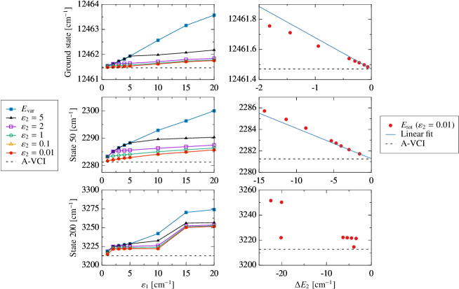
Figure 2: VHCI energy of the ground state (top row), the 50th state (middle row) and 200th state (bottom row) of ethylene oxide. The left-hand column shows the energy as a function of the variational heat-bath cutoff parameter ${\varepsilon}_{1}$ and includes the variational energy $E_{\mathrm{var}}$ (blue squares) and the total energy $E_{\mathrm{tot}}=E_{\mathrm{var}}+\Delta E_{2}$ for various values of the perturbative heat-bath screening parameter ${\varepsilon}_{2}$. The black dashed lines are the converged A-VCI values for each state, which can be considered to be exact. In the right-hand column, we present the total energy $E_{\mathrm{tot}}$ (red circles) with converged PT2 (${\varepsilon}_{2}=0.01$ cm^-1) as a function of the perturbative correction $\Delta E_{2}$. Note that we use a smaller y-range because the energy varies less with respect to ${\varepsilon}_{1}$ when the PT2 stage is converged. We also show the linear fits (blue lines) of the most accurate two points (${\varepsilon}_{1}=1$ and 2 cm^-1) for the ground state and state 50, which were used to find the extrapolated energies presented in Table 3.

Finally, following standard HCI practice in electronic structure, we attempt to approximate the exact energies via extrapolation. On the right-hand side of Fig. 2, we plot the VHCI+PT2 energy of each state as a function of the PT2 correction $\Delta E_{2}$ seeking to extrapolate to $\Delta E_{2}=0$, following Ref. 25. We see that extrapolation is reasonable and successful for low-lying states, but not for high-lying states. In general, extrapolation of high-lying states is difficult because the level spacing becomes very small and the states are highly multiconfigurational, such that tracking a single level as ${\varepsilon}_{1}$ changes is challenging. We performed extrapolation for the first 50 states using a linear fit to results obtained with ${\varepsilon}_{1}=1$ cm^-1 and 2 cm^-1, as shown graphically in the right-hand sides of Fig. 2 for the first and 50th states; we tested other polynomial fits and found linear extrapolation to be the simplest and best perfoming, although other schemes could be considered in the future. In Table 2, we present the extrapolated energies of the first ten states as well as the statistics of the first 50 states; all energies can be found in the supplementary material. The results are nearly exact, with a maximum AE below 0.1 cm^-1 for all 50 states, and obviously require no additional computing effort. We conclude that linear extrapolation of high-quality VHCI+PT2 energies is a powerful way to achieve nearly exact energies for the ground state and many low-lying excited states.

Table 4: Ten lowest- and ten highest-energy states from a calculation of the first 128 eigenstates of naphthalene, with excitation energies given relative to the ZPE. VHCI results are shown for two different values of ${\varepsilon}_{1}$ with no PT2 correction (Var) and with PT2 at ${\varepsilon}_{2}=0.2$ cm^-1. We compare to reference values from the smallest and largest HI-RRBPM calculations in Ref. 43 (“A” and “G” respectively) as well as to VASCI [36] with no PT2 correction and $N_{\mathcal{V}}$ similar to our ${\varepsilon}_{1}=1.5$ cm^-1 case. Assignments are given using the mode-numbering convention of Ref. 49. All energies are in cm^-1

Method:	${\varepsilon}_{1}=1.5$		${\varepsilon}_{1}=1.0$		VASCI [36]		HI-RRBPM [43]
$N_{\mathrm{\mathcal{V}}}$:	1 322 334		2 270 672		1 000 000	1 500 000	A	G
	Var	${\varepsilon}_{2}=0.2$	Var	${\varepsilon}_{2}=0.2$	Var	Var	Var	Var
ZPE	31772.71	31764.77	31769.90	31764.34	31774.4	31773.6	31782.20	31766.03
$\omega_{48}$	168.17	165.20	166.89	164.63	166.4	166.3	165.84	164.60
$\omega_{13}$	182.57	179.28	181.28	178.79	179.9	179.9	184.90	178.18
$2\omega_{48}$	335.22	329.48	333.17	328.69	336.4	336.1	338.21	329.41
$\omega_{13}+\omega_{48}$	349.25	342.84	346.48	341.76	349.5	349.4	365.68	342.02
$\omega_{24}$	358.59	356.26	357.83	355.97	361.4	363.8	372.86	354.44
$2\omega_{13}$	362.91	357.23	360.75	356.49	363.4	366.6	397.32	357.66
$\omega_{16}$	392.38	389.05	391.19	388.64	394.1	396.3	405.35	387.71
$\omega_{28}$	468.62	464.50	467.08	463.93	470.9	475.3	468.20	463.47
$\omega_{47}$	477.41	472.97	475.83	472.45	479.7	483.1	477.10	472.41
$3\omega_{48}$	503.57	493.98	499.45	492.38	502.5	501.8	506.60	495.50
$\omega_{13}+\omega_{23}$	978.99	972.19	976.88	971.60	991.6	1007.1	1091.20	974.99
$\omega_{24}+\omega_{36}$	982.41	977.49	981.37	977.64	1006.6	1015.4	1099.87	982.87
$\omega_{12}+\omega_{24}$	984.01	978.50	982.39	977.99	1002.2	1015.7	1100.56	985.06
$\omega_{9}+\omega_{28}$	984.89	978.67	982.83	978.03	997.7	1010.7	1098.74	981.31
$\omega_{44}+\omega_{47}$	986.66	979.81	984.23	979.12	1001.8	1013.3	1106.07	987.92
$\omega_{9}+\omega_{47}$	993.93	987.08	991.49	986.44	–	–	1121.57	994.66
$\omega_{35}$	1013.18	1008.63	1011.79	1008.21	–	–	1134.08	1011.99
$\omega_{16}+\omega_{36}$	1017.62	1011.96	1015.91	1011.51	–	–	1138.09	1013.55
$2\omega_{44}$	1017.51	1012.86	1016.19	1012.70	–	–	1138.46	1015.09
$\omega_{9}+\omega_{44}$	1024.79	1020.17	1023.43	1019.82	–	–	1148.79	1018.96
Max AE(25):	11.78	2.85	6.32	3.69	16.1	–	54.64	–
RMSE(25):	6.62	1.35	4.18	1.68	9.0	–	30.44	–
Core hours:	1234.4	2004.0	2620.8	3993.4	1584.7	1834.9	1167.4	63590.4
Cores:	20	20	20	20	40	40	128	64

III.5 Naphthalene: A 48-dimensional system

As a final test of VHCI, we consider naphthalene, C₁₀H₈, with 18 atoms and 48 normal modes, making it more than three times larger than any of the previous test systems. We use the quartic PES of Cané et al. [49], which was calculated at the B97-1/TZ2P level of theory, and includes 4125 nonzero anharmonic force constants. Large variational calculations were previously performed with this PES using the Hierarchical Intertwined Reduced-Rank Block Power Method (HI-RRBPM) [43]. We compare to the affordable HI-RRBPM (A) results and the most expensive HI-RRBPM (G) results, which we consider to be the most accurate. Finally, we compare to variational VASCI calculations from Ref. 36 with 1 million and 1.5 million basis states, obtained using 25 000 and 15 000 core states, respectively. Following Refs. 43, 36, we calculate the 128 lowest states of naphthalene, of which the ten lowest and ten highest are presented in Table 4; results for all states can be found in the supplementary material. We show results with VHCI variational cutoff values ${\varepsilon}_{1}=1.5$ cm^-1 and 1 cm^-1, producing approximately 1.3 million and 2.3 million basis states, respectively. Although a fully converged PT2 correction is intractable, we calculate an approximate PT2 correction with heat-bath screening; we used ${\varepsilon}_{2}=0.2$ cm^-1, producing a perturbative space containing approximately 15 million states.

For low-lying states, the agreement between variational VHCI and HI-RRBPM (G) is very good. At comparable computational cost, the accuracy of variational VASCI and VHCI is similar. The PT2 correction to VHCI produces a significant improvement of low-lying energies, which now match HI-RRBPM (G) to an accuracy of about 1 cm^-1.

We calculated the maximum absolute error and RMSE with respect to HI-RRBPM for the first 25 eigenstates. We matched the states to Ref. 43 and Ref. 36 according to their mode assignments. Variational VHCI achieves marginally closer agreement to the large HI-RRBPM(G) calculation than VASCI. Perturbation theory provides a noticeable improvement over the variational result. Curiously, VHCI+PT2 produces a more accurate result for the smaller variational space, indicating that the calculation is probably not converged with respect to ${\varepsilon}_{2}$. Indeed, ideally the PT2 correction should be calculated with ${\varepsilon}_{2}\ll{\varepsilon}_{1}$, but even ${\varepsilon}_{2}=0.2$ cm^-1 produces an accurate result for low-lying states. As a convergence test, we also performed a large VHCI calculation that optimizes only the ground state (not shown), and obtained a variational ZPE that is at least 4 cm^-1 lower than the HI-RRBPM (G) answer; therefore, some of our VHCI results that are lower than HI-RRBPM (G) may actually be more accurate, which would explain some of the discrepancies seen in the comparison.

For the high-lying states, which are much harder to converge as we discussed above, we only present results for those states that match the mode assignment from HI-RRBPM (G) and we do not attempt to calculate error statistics. For states with matching assignments, we see good agreement between variational VHCI and HI-RRBPM (G), especially at ${\varepsilon}_{1}=1$ cm^-1. The PT2 correction is not as helpful for high-lying states as it is for low-lying ones, because the variational space of the low-lying states is tightly converged and additional corrections are well-captured by perturbation theory. In some cases, the PT2 correction worsens the agreement with HI-RRBPM (G), although this may be a result of an incorrect mode assignment inside a dense spectrum of excited states. We do not attempt any extrapolation because ${\varepsilon}_{2}=0.2$ cm^-1 is not small enough to converge the PT2 correction; a stochastic PT2 implementation [26] would be clearly beneficial. Overall, we are confident that the eigenvalue spectrum obtained from our VHCI calculations is accurate enough to be useful in real-world applications. Comparison of the overall CPU times, presented at the bottom of Table 4, underscores the competitiveness of VHCI as a means of accurately solving the vibrational Schrödinger equation on high-dimensional anharmonic potentials.

IV Conclusions

We have introduced vibrational heat-bath configuration interaction based on the original principles of HCI [24], but with adaptations for vibrational Hamiltonians. VHCI+PT2 performed well on our four test molecules, achieving quantitative accuracy for the 12-dimensional systems acetonitrile and ethylene, while outperforming VASCI and vDMRG. VHCI also performed well on larger systems, especially for low-lying states. High-lying states are a challenge due to their highly multi-configurational character and dense energetic spacing. Convergence of high-lying states could be improved by implementing a state-specific algorithm [31, 32, 33].

In future work, the implementation of semistochastic PT2 [26, 25, 27] will be critical for studying even larger systems. Furthermore, VHCI can be straightforwardly extended to efficiently calculate spectroscopic intensities based on the dipole moment surface [50, 51, 33]. Consideration of spectroscopic activity can also be used to target eigenstates more efficiently, as recently implemented in A-VCI [52]. Finally, it will be interesting to apply VHCI to more strongly anharmonic systems, such as molecular clusters [53, 54] or floppy molecules [55, 56, 4], where truncated expansions of the PES may not be sufficient.

Supplementary material

See the supplementary material for VHCI energies and assignments of all states calculated for the four molecules considered in this work.

Data availability statement

The software and data that support the findings of this study are openly available in the supplementary material and in our GitHub repository at https://github.com/berkelbach-group/VHCI with digital object identifier 10.5281/zenodo.4116070.

References

- B. Gerber et al. [2002] R. B. Gerber, B. Brauer, S. K. Gregurick, and G. M. Chaban, “Calculation of anharmonic vibrational spectroscopy of small biological molecules,” PhysChemComm 5, 142 (2002).
- Chaban, Jung, and Benny Gerber [1999] G. M. Chaban, J. O. Jung, and R. Benny Gerber, “Ab initio calculation of anharmonic vibrational states of polyatomic systems: Electronic structure combined with vibrational self-consistent field,” J. Chem. Phys. 111, 1823–1829 (1999).
- Carter, Culik, and Bowman [1997] S. Carter, S. J. Culik, and J. M. Bowman, “Vibrational self-consistent field method for many-mode systems: A new approach and application to the vibrations of CO adsorbed on Cu(100),” J. Chem. Phys. 107, 10458–10469 (1997).
- Roy and Gerber [2013] T. K. Roy and R. B. Gerber, “Vibrational self-consistent field calculations for spectroscopy of biological molecules: new algorithmic developments and applications,” Phys. Chem. Chem. Phys. 15, 9468 (2013).
- Barone [2005] V. Barone, “Anharmonic vibrational properties by a fully automated second-order perturbative approach,” J. Chem. Phys. 122 (2005), 10.1063/1.1824881.
- Christiansen [2003] O. Christiansen, “Møller-Plesset perturbation theory for vibrational wave functions,” J. Chem. Phys. 119, 5773–5781 (2003).
- Sibert [1987] E. L. Sibert, “Theoretical studies of vibrationally excited polyatomic molecules using canonical Van Vleck perturbation theory,” J. Chem. Phys. 88, 4378–4390 (1987).
- Banik, Pal, and Prasad [2008] S. Banik, S. Pal, and M. D. Prasad, “Calculation of vibrational energy of molecule using coupled cluster linear response theory in bosonic representation: Convergence studies,” J. Chem. Phys. 129 (2008), 10.1063/1.2982502.
- Seidler and Christiansen [2009] P. Seidler and O. Christiansen, “Automatic derivation and evaluation of vibrational coupled cluster theory equations,” J. Chem. Phys. 131 (2009), 10.1063/1.3272796.
- Christiansen [2004] O. Christiansen, “Vibrational coupled cluster theory,” J. Chem. Phys. 120, 2149–2159 (2004).
- Bowman, Christoffel, and Tobin [1979] J. M. Bowman, K. Christoffel, and F. Tobin, “Application of SCF-SI theory to vibrational motion in polyatomic molecules,” J. Phys. Chem. 83, 905–920 (1979).
- Thompson and Truhlar [1980] T. C. Thompson and D. G. Truhlar, “SCF CI calculations for vibrational eigenvalues and wavefunctions of systems exhibiting fermi resonance,” Chem. Phys. Lett. 75, 87–90 (1980).
- Christoffel and Bowman [1982] K. M. Christoffel and J. M. Bowman, “Investigations of self-consistent field, scf ci and virtual stateconfiguration interaction vibrational energies for a model three-mode system,” Chem. Phys. Lett. 85, 220–224 (1982).
- Avila and Carrington [2011] G. Avila and T. Carrington, “Using nonproduct quadrature grids to solve the vibrational Schrödinger equation in 12D,” J. Chem. Phys. 134, 054126 (2011).
- Leclerc and Carrington [2014] A. Leclerc and T. Carrington, “Calculating vibrational spectra with sum of product basis functions without storing full-dimensional vectors or matrices,” J. Chem. Phys. 140, 174111 (2014).
- Odunlami et al. [2017] M. Odunlami, V. Le Bris, D. Bégué, I. Baraille, and O. Coulaud, “A-VCI: A flexible method to efficiently compute vibrational spectra,” J. Chem. Phys. 146, 214108 (2017).
- Baiardi et al. [2017] A. Baiardi, C. J. Stein, V. Barone, and M. Reiher, “Vibrational Density Matrix Renormalization Group,” J. Chem. Theory Comput. 13, 3764–3777 (2017).
- Huron, Malrieu, and Rancurel [1973] B. Huron, J. P. Malrieu, and P. Rancurel, “Iterative perturbation calculations of ground and excited state energies from multiconfigurational zeroth‐order wavefunctions,” J. Chem. Phys. 58, 5745–5759 (1973).
- Buenker and Peyerimhoff [1974] R. J. Buenker and S. D. Peyerimhoff, “Individualized configuration selection in CI calculations with subsequent energy extrapolation,” Theor. Chim. Acta 35, 33–58 (1974).
- Harrison [1991] R. J. Harrison, “Approximating full configuration interaction with selected configuration interaction and perturbation theory,” J. Chem. Phys. 94, 5021–5031 (1991).
- Schriber and Evangelista [2016] J. B. Schriber and F. A. Evangelista, “Communication: An adaptive configuration interaction approach for strongly correlated electrons with tunable accuracy,” J. Chem. Phys. 144, 161106 (2016).
- Tubman et al. [2016] N. M. Tubman, J. Lee, T. Y. Takeshita, M. Head-Gordon, and K. B. Whaley, “A deterministic alternative to the full configuration interaction quantum Monte Carlo method,” J. Chem. Phys. 145 (2016), 10.1063/1.4955109.
- Tubman et al. [2020] N. M. Tubman, C. D. Freeman, D. S. Levine, D. Hait, M. Head-Gordon, and K. B. Whaley, “Modern Approaches to Exact Diagonalization and Selected Configuration Interaction with the Adaptive Sampling CI Method,” J. Chem. Theory Comput. 16, 2139–2159 (2020).
- Holmes, Tubman, and Umrigar [2016] A. A. Holmes, N. M. Tubman, and C. J. Umrigar, “Heat-Bath Configuration Interaction: An Efficient Selected Configuration Interaction Algorithm Inspired by Heat-Bath Sampling,” J. Chem. Theory Comput. 12, 3674–3680 (2016).
- Holmes, Umrigar, and Sharma [2017] A. A. Holmes, C. J. Umrigar, and S. Sharma, “Excited states using semistochastic heat-bath configuration interaction,” J. Chem. Phys. 147, 164111 (2017).
- Sharma et al. [2017] S. Sharma, A. A. Holmes, G. Jeanmairet, A. Alavi, and C. J. Umrigar, “Semistochastic Heat-Bath Configuration Interaction Method: Selected Configuration Interaction with Semistochastic Perturbation Theory,” J. Chem. Theory Comput. 13, 1595–1604 (2017).
- Li et al. [2018] J. Li, M. Otten, A. A. Holmes, S. Sharma, and C. J. Umrigar, “Fast semistochastic heat-bath configuration interaction,” J. Chem. Phys. 149, 214110 (2018).
- Williams et al. [2020] K. T. Williams, Y. Yao, J. Li, L. Chen, H. Shi, M. Motta, C. Niu, U. Ray, S. Guo, R. J. Anderson, J. Li, L. N. Tran, C. N. Yeh, B. Mussard, S. Sharma, F. Bruneval, M. Van Schilfgaarde, G. H. Booth, G. K. L. Chan, S. Zhang, E. Gull, D. Zgid, A. Millis, C. J. Umrigar, and L. K. Wagner, “Direct Comparison of Many-Body Methods for Realistic Electronic Hamiltonians,” Phys. Rev. X 10, 11041 (2020).
- Yao et al. [2020] Y. Yao, E. Giner, J. Li, J. Toulouse, and C. J. Umrigar, “Almost exact energies for the Gaussian-2 set with the semistochastic heat-bath configuration interaction method,” J. Chem. Phys. 153, 124117 (2020).
- Eriksen et al. [2020] J. J. Eriksen, T. A. Anderson, J. E. Deustua, K. Ghanem, D. Hait, M. R. Hoffmann, S. Lee, D. S. Levine, I. Magoulas, J. Shen, N. M. Tubman, K. B. Whaley, E. Xu, Y. Yao, N. Zhang, A. Alavi, G. K.-L. Chan, M. Head-Gordon, W. Liu, P. Piecuch, S. Sharma, S. L. Ten-no, C. J. Umrigar, and J. Gauss, “The Ground State Electronic Energy of Benzene,” J. Phys. Chem. Lett. , 8922–8929 (2020).
- Rauhut [2007] G. Rauhut, “Configuration selection as a route towards efficient vibrational configuration interaction calculations,” J. Chem. Phys. 127 (2007), 10.1063/1.2790016.
- Neff and Rauhut [2009] M. Neff and G. Rauhut, “Toward large scale vibrational configuration interaction calculations,” J. Chem. Phys. 131 (2009), 10.1063/1.3243862.
- Carbonnière, Dargelos, and Pouchan [2010] P. Carbonnière, A. Dargelos, and C. Pouchan, “The VCI-P code: An iterative variation-perturbation scheme for efficient computations of anharmonic vibrational levels and IR intensities of polyatomic molecules,” Theor. Chem. Acc. 125, 543–554 (2010).
- Sibaev and Crittenden [2016a] M. Sibaev and D. L. Crittenden, “Balancing accuracy and efficiency in selecting vibrational configuration interaction basis states using vibrational perturbation theory,” J. Chem. Phys. 145, 064106 (2016a).
- Scribano and Benoit [2008] Y. Scribano and D. M. Benoit, “Iterative active-space selection for vibrational configuration interaction calculations using a reduced-coupling VSCF basis,” Chem. Phys. Lett. 458, 384–387 (2008).
- Lesko, Ardiansyah, and Brorsen [2019] E. Lesko, M. Ardiansyah, and K. R. Brorsen, “Vibrational adaptive sampling configuration interaction,” J. Chem. Phys. 151, 164103 (2019).
- Garnier et al. [2016] R. Garnier, M. Odunlami, V. Le Bris, D. Bégué, I. Baraille, and O. Coulaud, “Adaptive vibrational configuration interaction (A-VCI): A posteriori error estimation to efficiently compute anharmonic IR spectra,” J. Chem. Phys. 144, 1–4 (2016).
- Kratz [2016] E. G. Kratz, “LOVCI: Ladder operator vibrational configuration iteraction,” https://github.com/kratman/VibCI (2016).
- Fetherolf [2020] J. H. Fetherolf, “VHCI: Vibrational heat-bath configuration interaction v0.1,” https://github.com/berkelbach-group/VHCI (2020).
- Guennebaud, Jacob et al. [2010] G. Guennebaud, B. Jacob, et al., “Eigen v3,” http://eigen.tuxfamily.org (2010).
- Qiu [2015] Y. Qiu, “SPECTRA: Sparse eigenvalue computation toolkit as a redesigned ARPACK,” https://spectralib.org/ (2015).
- Brown and Carrington [2016] J. Brown and T. Carrington, “Using an expanding nondirect product harmonic basis with an iterative eigensolver to compute vibrational energy levels with as many as seven atoms,” J. Chem. Phys. 145, 144104 (2016).
- Thomas et al. [2018] P. S. Thomas, T. Carrington, J. Agarwal, and H. F. Schaefer, “Using an iterative eigensolver and intertwined rank reduction to compute vibrational spectra of molecules with more than a dozen atoms: Uracil and naphthalene,” J. Chem. Phys. 149 (2018), 10.1063/1.5039147.
- Begue, Carbonniere, and Pouchan [2005] D. Begue, P. Carbonniere, and C. Pouchan, “Calculations of Vibrational Energy Levels by Using a Hybrid ab Initio and DFT Quartic Force Field: Application to Acetonitrile,” J. Phys. Chem. A 109, 4611–4616 (2005).
- Delahaye et al. [2014] T. Delahaye, A. Nikitin, M. Rey, P. G. Szalay, and V. G. Tyuterev, “A new accurate ground-state potential energy surface of ethylene and predictions for rotational and vibrational energy levels,” J. Chem. Phys. 141 (2014), 10.1063/1.4894419.
- Sibaev and Crittenden [2015] M. Sibaev and D. L. Crittenden, “The PyPES library of high quality semi-global potential energy surfaces,” J. Comput. Chem. 36, 2200–2207 (2015).
- Sibaev and Crittenden [2016b] M. Sibaev and D. L. Crittenden, “PyVCI: A flexible open-source code for calculating accurate molecular infrared spectra,” Comput. Phys. Commun. 203, 290–297 (2016b).
- Bégué et al. [2007] D. Bégué, N. Gohaud, C. Pouchan, P. Cassam-Chenaï, and J. Liévin, “A comparison of two methods for selecting vibrational configuration interaction spaces on a heptatomic system: Ethylene oxide,” J. Chem. Phys. 127, 164115 (2007).
- Cané, Miani, and Trombetti [2007] E. Cané, A. Miani, and A. Trombetti, “Anharmonic force fields of naphthalene-h8 and naphthalene-d 8,” J. Phys. Chem. A 111, 8218–8222 (2007).
- Baraille et al. [2001] I. Baraille, C. Larrieu, A. Dargelos, and M. Chaillet, “Calculation of non-fundamental IR frequencies and intensities at the anharmonic level. I. The overtone, combination and difference bands of diazomethane, H2CN2,” Chem. Phys. 273, 91–101 (2001).
- Burcl, Carter, and Handy [2003] R. Burcl, S. Carter, and N. C. Handy, “Infrared intensities from the MULTIMODE code,” Chem. Phys. Lett. 380, 237–244 (2003).
- Le Bris et al. [2020] V. Le Bris, M. Odunlami, D. Bégué, I. Baraille, and O. Coulaud, “Using computed infrared intensities for the reduction of vibrational configuration interaction bases,” Phys. Chem. Chem. Phys. 22, 7021–7030 (2020).
- Kim, Jordan, and Zwier [1994] K. Kim, K. D. Jordan, and T. S. Zwier, “Low-Energy Structures and Vibrational Frequencies of the Water Hexamer: Comparison with Benzene-(H2O)6,” J. Am. Chem. Soc. 116, 11568–11569 (1994).
- Yu and Bowman [2019] Q. Yu and J. M. Bowman, “Classical, Thermostated Ring Polymer, and Quantum VSCF/VCI Calculations of IR Spectra of H 7 O 3 + and H 9 O 4 + (Eigen) and Comparison with Experiment,” J. Phys. Chem. A 123, 1399–1409 (2019).
- Bačić and Light [1989] Z. Bačić and J. C. Light, “Theoretical Methods For Rovibrational States Of Floppy Molecules,” Annu. Rev. Phys. Chem. 40, 469–498 (1989).
- Bramley et al. [1994] M. J. Bramley, J. W. Tromp, T. Carrington, and G. C. Corey, “Efficient calculation of highly excited vibrational energy levels of floppy molecules: The band origins of h + 3 up to 35 000 cm -1,” J. Chem. Phys. 100, 6175–6194 (1994).