Nonexistence of Invariant Tori Transverse to Foliations:
An Application of Converse KAM Theory

Abstract

Invariant manifolds are of fundamental importance to the qualitative understanding of dynamical systems. In this work, we explore and extend MacKay’s converse KAM condition to obtain a sufficient condition for the nonexistence of invariant surfaces that are transverse to a chosen 1D foliation. We show how useful foliations can be constructed from approximate integrals of the system. This theory is implemented numerically for two models, a particle in a two-wave potential and a Beltrami flow studied by Zaslavsky (Q-flows). These are both 3D volume-preserving flows, and they exemplify the dynamics seen in time-dependent Hamiltonian systems and incompressible fluids, respectively. Through both numerical and theoretical considerations, it is revealed how to choose foliations that capture the nonexistence of invariant tori with varying homologies.

Kolmogorov-Arnold-Moser (KAM) theory provides conditions under which a nearly-integrable Hamiltonian system or symplectic map can be guaranteed to have invariant tori on which the dynamics is conjugate to rigid rotations. Dynamical behavior on these invariant sets is just like that of an integrable system, for which the phase space is almost everywhere foliated by such tori. By contrast, converse KAM theory, as initiated by Mather in 1984, seeks to obtain conditions for the nonexistence of invariant tori. Mather’s idea is based on the fact that if a two-dimensional map has an invariant circle, then the iterates of an infinitesimal vector that is attached to a point on the circle cannot rotate through the tangent space of the circle. A converse KAM condition then becomes: no such circle can exist if a vector rotates “too much”. This condition was also extended to flows by MacKay, who gave a condition for the nonexistence of “rotational” invariant tori on three-dimensional energy surfaces of a two degree-of freedom Hamiltonian system.
Here we use MacKay’s ideas to explore the definition of rotation relative to a choice of foliation—a family of curves that cover the manifold. A codimension-one torus that is transverse to the foliation is ruled out when a positive tangent vector to the foliation flows past a negative one–exceeding a half rotation. Selection of the foliation is crucial in detecting the nonexistence of tori that might have different topological structures. We explore choosing foliations based on gradients of approximate invariants for several examples of flows in three dimensions.

I Introduction

Mather’s converse KAM theory Mat (84, 86) is based on a theorem due to Birkhoff: for an area and orientation-preserving twist (or more generally, tilt) map, $f:M\to M$, on $M=\mathbb{T}\times\mathbb{R}$, every rotational invariant circle is a Lipschitz graph over the angle variable Mat (84); Mei (92). Recall that a set $\mathcal{C}\subset M$ is invariant when $f(\mathcal{C})=\mathcal{C}$ and it is a rotational circle if it is homotopic to the horizontal circle $\{(x,0)\,|\,x\in\mathbb{T}\}$. The implication is that, if $v\in TM_{z}$ is a tangent vector at a point $z=(x,y)\in M$ to a rotational invariant circle $\mathcal{C}$, then it is contained in a Lipschitz cone.

Constraining the tangent vectors to a Lipschitz cone can be turned into a nonexistence condition in the following way. Consider a point $z_{0}\in M$ and an arbitrary vector $\xi_{0}\in T_{z_{0}}M$. If there is a rotational invariant circle $\mathcal{C}$ that contains $z_{0}$, then under iteration by linearized map $Df_{z_{t}}:T_{z_{t}}M\to T_{z_{t+1}}M$, this vector $\xi_{0}$ cannot cross the circle. Indeed, since the tangent to the circle lies in the Lipschitz cone, the image at time $t$, $\xi_{t}:=Df_{z_{t-1}}\xi_{t-1}$, cannot cross this cone. The simplest manifestation of this is that an initially vertical vector $\xi_{0}=(0,1)^{T}$ can never rotate past the negative vertical $(0,-1)^{T}$. For example, when the twist is positive, vertical vectors tilt to the right, so if there is a $t$ for which $\xi_{t}$ is in the third quadrant, there is no invariant circle through $z_{0}$. This gives a sufficient condition for nonexistence of a rotational circle.

Mather used this nonexistence condition, together with explicit Lipschitz bounds, to show that there are no rotational invariant circles for Chirikov’s standard map when $k>4/3$; this amazing result is not too far from the numerically obtained value $k_{cr}\approx 0.971$, for the last such circle Gre (79). Using interval arithmetic, MacKay and Percival MP (85) showed nonexistence for $k>63/64$. Subsequent calculations have improved this bound Jun (91).

This converse KAM condition has been generalized to higher-dimensional, symplectic maps with nondegenerate twist MMS (89) and monotone-positive, exact-symplectic maps Har (99), as well as to Hamiltonian systems on a cotangent bundle that satisfy a Legendre condition Mac (89). In these cases, the criteria can rule out the existence of tori that are Lagrangian graphs. Note, however, that for the higher-dimensional case there is no generalization of Birkhoff’s theorem: it is not clear that all rotational tori are indeed Lagrangian graphs, even when an analogue of the twist condition is satisfied.

Other applications include a study of the tilting of a rigid body in an elliptical Kepler orbit for both conservative and dissipative cases CM (07). This system is effectively three-dimensional, and the authors use the conjugate point technique of Mac (89) to compute regions of phase space that cannot contain rotational tori. Ideas similar to the converse KAM theorem show that in a “natural Hamiltonian system” (of kinetic plus potential energy form), any compact energy surface cannot be completely foliated by invariant $n$-tori Kna (90). Another result for these natural systems gives a criterion for the nonexistence of so-called “viscosity solutions” to the Hamilton-Jacobi equation GO (08).

White introduces an analogous condition in a study of guiding center dynamics Whi (11, 12, 15). This two degree-of-freedom Hamiltonian system can be reduced to an area-preserving map on an energy surface by taking a Poincaré section. In this work, instead of utilizing the tangent map idea of Mather, White computes a nearby trajectory $z^{*}_{t}$ to $z_{t}$ and studies the finite-size vector $\Delta z_{t}^{*}=z^{*}_{t}-z_{t}$. A similar converse KAM theorem still holds; if $\Delta z_{t}^{*}$ rotates by more than $\pi$, then $z_{t}$ does not lie on a rotational invariant torus. White calls his method “phase vector rotation”. Analyzing this finite-size vector $\Delta z_{t}^{*}$ has a deficiency that Mather’s tangent map does not. Consider the dynamics of a pendulum and suppose that $z_{t}$ is on a librational torus, so it oscillates about the stable equilibrium, but that $z_{t}^{*}$ is instead chosen to be on the other side of the separatrix, on a rotational torus. Then, in such a situation, $\Delta z_{t}^{*}$ will not necessarily rotate by more than $\pi$ — it could remain more-or-less vertical throughout the evolution. Thus, $z_{0}$ would not satisfy the phase vector rotation condition and hence it could not be concluded to not lie on a rotational torus. The implication is that one must be careful in interpreting the results of this method. We will use below a useful diagnostic that White introduces: a plot of the effective rotation rate as a function of initial condition.

A reformulation of the converse KAM condition was given by MacKay Mac (18) for three-dimensional flows, the context that we will be working on in this paper. In particular, we will numerically explore a key result of MacKay (Mac, 18, thm. 1). Given a flow $\phi$ generated by a $C^{1}$ vector field $v$ on some $n$-dimensional manifold $M$, MacKay finds conditions under which a given point $x\in M$ does not lie on an invariant, codimension-one, orientable surface $S$. The class of surfaces considered are those that are everywhere transverse to the leaves of a given one-dimensional, orientable foliation $\mathcal{F}$ of $M$. Recall that a $k$-dimensional foliation is an equivalence relation on the manifold $M$, where the equivalence classes, called leaves, are injectively immersed submanifolds of dimension $k$. Essentially $\mathcal{F}$ is a collection of disjoint $k$-dimensional submanifolds whose union is the manifold $M$.

Given a choice of foliation $\mathcal{F}$, we use the theorem of MacKay to construct a numerical scheme that detects the nonexistence of invariant surfaces transverse to the foliation. This scheme is applied to two models. The first is the two-wave model, which is perhaps the simplest nonintegrable, nonlinear, $1\tfrac{1}{2}$ degree-of-freedom Hamiltonian system. This model was also studied by MacKay using the vertical foliation Mac (89); here we will compare several foliations. The second model is a family of incompressible, Beltrami flows that were called Q-flows by Zaslavsky Zas (91). These vector fields can have crystalline or quasi-crystalline spatial symmetries. Zaslavsky studied anomalous diffusion in these systems, but converse KAM theory has not been previously applied.

Using these two models, we investigate methods for choosing an appropriate 1D foliation and reveal some of the consequences of such a choice. In particular, if the 1D foliation is generated from the gradient flow of a function $J:M\to\mathbb{R}$ , we are able to test for the nonexistence of invariant tori that are not of null-homology on the manifold $M\setminus\Sigma$, where $\Sigma$ is the set of singular leaves of $J$.

In §II we introduce the concepts and background for converse KAM theory. The main result of MacKay, Thm. II.3, is recalled and a simplification for Cartan-Arnol’d type systems is obtained. The two models that we study are described in §III. In §IV we discuss the construction of a number of foliations for each model and give a description of techniques used to numerically implement Thm. II.3. The results of numerical experiments are given in §V and discussed in §VI.

II Converse KAM Theorem: Background and Theory

In this section we will expand on some details of Mac (18), prove several helpful results, and discuss the generation of foliations from the gradient flow of an approximate integral.

We will study the flow $\phi$ of a $C^{1}$ vector field $v$ on an orientable manifold $M$:

$$\frac{d}{dt}\phi_{t}(x)=v(\phi_{t}(x)),\quad\phi_{0}(x)=x,$$ (1)

That is, we assume that $\phi$ is a complete flow on $M$. In our applications, $M$ will be three-dimensional and $v$ will either be Hamiltonian or divergence-free. However, at first, we more generally assume that $M$ is $n$-dimensional and $v$ is a general vector field on $M$.

II.1 Surfaces Transverse to a Foliation

Let $\mathcal{F}$ be a given 1D foliation on $M$ and denote the leaf at a point $x$ by $\mathcal{F}_{x}$. We begin by recalling the definition of a transverse surface to $\mathcal{F}$.

Definition (Transverse Surfaces).

Let $\mathcal{F}$ be a one-dimensional foliation of a manifold $M$. A codimension-one surface $S$ in $M$ is transverse to $\mathcal{F}$ if, for every point $x\in S$, the tangent space $T_{x}S$ does not contain the tangent space of the foliation $\mathcal{F}$ at $x$: $T_{x}\mathcal{F}\nsubseteq T_{x}S$.

Locally, there always exists an $n-1$ dimensional submanifold $B$ transverse to the leaves of $\mathcal{F}$. In other words, $\mathcal{F}$ is locally diffeomorphic to the trivial fibre bundle $B\times\mathbb{R}$. By definition, a surface $S$ is locally transverse to the leaves of $\mathcal{F}$ if and only if $S$ is locally a graph over $B$. This follows from the converse of the implicit function theorem; indeed, if there is some point $x\in M$ for which the tangent space $T_{x}S$ contains the tangent space of the foliation at $x$, $T_{x}\mathcal{F}$ then $S$ is not locally a $C^{1}$ graph over $B$.

When $S$ is invariant under the flow (1), we can use the vector field $v$ to help detect transversality:

Lemma II.1.

Suppose that $S$ is a surface that is invariant under (1); that is, for each $x\in S$, $v(x)\in T_{x}S$. Let $\eta$ be any nonzero vector field in $\mathcal{F}$ and $y$ be a point in $S$ for which $v(y)\neq 0$. Then if either

1. $\eta_{y}=cv(y)$, for some $c\neq 0$ or,

2. there exists some $s\in T_{y}S$ independent of $v(y)$ such that $\eta_{y}=s+cv(y)$,

then $S$ is not transverse to $\mathcal{F}$.

Proof.

Since invariance implies that $v(x)\in T_{x}S$, if there is a vector $s\in T_{y}S$ such that $\eta_{y}=s+cv(y)$ for some $c\in\mathbb{R}$ then $T_{y}\mathcal{F}_{y}\subset T_{y}S$. This is true whenever either (1) or (2) is true. ∎

Note that if the first condition in Lem. II.1 is true, it follows that $\mathcal{F}_{y}$ is not transverse to the vector field $v(y)$. This condition is easy to check analytically. Unfortunately, the second condition can only be checked if we already know $S$. However, knowing $S$ in advance is clearly inconsistent with our goal of deciding if such a surface actually exists! What is needed is a systematic way of ruling out potential vectors $s$.

Under the assumption that the invariant surface $S$ and the foliation $\mathcal{F}$ are both orientable we can make progress toward eliminating potential tangent vectors. We start by choosing some volume form $\Omega$ in a tubular neighbourhood of $S$. The existence of $\Omega$ is guaranteed as $S$ is orientable, thus, the tubular neighbourhood is orientable, and all orientable manifolds have a volume form. This form need not be invariant under the flow $\phi$. Take a point $x_{0}\in S$ and let $x_{t}:=\phi_{t}(x_{0})$ denote its orbit. At each point $x_{t}$ consider a basis $s_{i}^{t},i=1\ldots n-2$, so that

$$\operatorname{Span}\{s_{1}^{t},\dots,s^{t}_{n-2},v(x_{t})\}=T_{x_{t}}S,$$ (2)

and let $\eta_{t}\in T_{x_{t}}\mathcal{F}$ be a nonzero vector field tangent to the orientable foliation. We assume that both the bases $s_{i}^{t}$ and the vector $\eta_{t}$ are at least $C^{0}$ for $t\in I\subset\mathbb{R}$ some interval.

If the orientable surface $S$ is transverse to $\mathcal{F}$, then an orientation of $\eta_{t}$ can be chosen such that

$$\Omega(\eta_{t},s_{1}^{t},\dots,s_{n-2}^{t},v(x_{t}))>0,\quad\forall t\in I.$$ (3)

Indeed, continuity of the basis and vector field $\eta_{t}$ implies that the sign of (3) must remain constant. If condition (3) were to fail, then $\mathcal{F}$ is not transverse to the tangent space (2) at the point $x_{t}$, and so the surface $S$ cannot be transverse to $\mathcal{F}$.

Since $S$ is also invariant, a second requirement can be deduced. Let $\xi_{0}\in T_{x_{0}}\mathcal{F}$ and

$${eq:linearization}\xi_{t}:=\phi_{t*}\xi_{0}=D_{x_{0}}\phi_{t}(x_{0})\xi_{0}\in T_{x_{t}}M;$$ (4)

be the pushforward of $\xi_{0}$ under the flow $\phi_{t}$, as sketched in Fig. 1. Note that, in general, $\xi_{t}\notin T_{x_{t}}\mathcal{F}$. The invariance of $S$, together with orientability, guarantee that

$$\Omega(\xi_{t},s_{1}^{t},\dots,s^{t}_{n-2},v(x_{t}))>0.$$ (5)

If condition (5) were to fail then either $S$ is not orientable or is not transverse to $\mathcal{F}$.

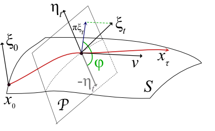
Figure 1: A sketch of a potential invariant surface $S$, the evolution of a vector $\xi_{0}$, to time $t$, and the local tangent $\eta_{t}$ to the foliation at $x_{t}$. A surface $\mathcal{P}$ transverse to $v(x_{t})$ gives a projection $\pi\xi_{t}$ along $v$, and the angle $\varphi$ (8). Here, $\mathcal{P}$ is chosen to contain $\mathcal{F}$.

These two conditions, (3) and (5), can be combined to imply

$$\Omega(c\eta_{t}+\xi_{t},s_{1}^{t},\dots,s^{t}_{n-2},v(x_{t}))>0,\qquad\forall c>0.$$ (6)

From the previous arguments, failure of (6) to hold implies that $x$ does not lie on an invariant, orientable surface $S$ transverse to $\mathcal{F}$ and with the given tangent space $\operatorname{Span}\{s_{1}^{t},\dots,s_{n-1}^{t}\}$.

In particular, if there is a time $t\in I$, such that $\xi_{t}=-c\eta_{t}+s$ where $\eta_{t}\in T_{x_{t}}\mathcal{F}$ and $s\in T_{x_{t}}S$, then condition (6) will fail. As we don’t know a priori if such an $s$ exists, all that can be checked is the case $s=dv(x_{t})$, that is, when $\xi_{t}=-c\eta_{t}+dv(x_{t})$ for some $c>0,d\in\mathbb{R}$.

This last result is still not computationally friendly, as one would need to check all possible coefficients $c$ and $d$ for each $t\in I$. To help avoid this, suppose that we can construct some $n-1$ dimensional foliation $\mathcal{P}$ that is transverse to $v$: we might think of $\mathcal{P}$ as a Poincaré foliation as it could lead to a local Poincaré section, recall Fig. 1. If we define the projection along $v(x)$ by $\pi:T_{x}M\to T_{x}\mathcal{P}_{x}$, then the condition $\xi_{t}=-c\eta_{t}+dv(x)$ becomes

$$\pi\xi_{t}=-c\pi\eta_{t}.$$ (7)

If $M$ has a Riemannian metric, the corresponding inner product $\langle\cdot,\cdot\rangle$ on each tangent space can be used to instead consider the angle

$$\varphi_{t}:=\cos^{-1}\left(\frac{\langle\pi\xi_{t},-\pi\eta_{t}\rangle}{\|\pi\xi_{t}\|\|\pi\eta_{t}\|}\right)\in[0,\pi],$$ (8)

as sketched in Fig. 1. Now (7) is equivalent to $\varphi_{t}=0$. Essentially we have the following extension of (Mac, 18, Thm. 1).

Theorem II.2.

Assume that $M$ is a manifold with dimension $n\geq 3$, $\mathcal{F}$ is an orientable 1D foliation, and $\mathcal{P}$ is a codimension-one Poincaré foliation containing $\mathcal{F}$. Given $x\in M$, a positively oriented tangent $\xi$ to $\mathcal{F}_{x}$ and the projection $\pi$, if there is some $t\in I\subset\mathbb{R}$ for which $\varphi_{t}=0$, then $x$ does not lie on any oriented, invariant $n-1$ dimensional sub-manifold of $M$ that is transverse to $\mathcal{F}$.

However, checking the hypotheses of Thm. II.2 is only reasonable for $n=3$. The issue is one of codimension: since each leaf of $\mathcal{P}$ is $n-1$ dimensional, checking that $\pi\xi_{t}=-c\pi\eta_{t}$ is equivalent to checking if a point crosses a codimension $n-2$ surface. Numerically, this can only be ascertained if the codimension of the crossed surface is $1$, that is, when $n=3$.

When $n=3$, we can refine Thm. II.2. Let,

$$\theta_{t}=\angle(\pi\xi_{t},-\pi\eta_{t})\in(-\pi,\pi]$$ (9)

be the oriented angle between $\pi\xi_{t}$ and $-\eta_{t}$. Note that computing the full-range angle is only possible if the two vectors are always in some given two-dimensional plane. If this angle crosses zero at some time, then we must have $\pi\xi_{t}=-\pi\eta_{t}$ at an earlier time. This leads to a mild extension of the original theorem of Mac (18).

Theorem II.3.

Mac (18) Assume that $M$ is a 3D manifold. Given $x\in M$, positively oriented tangent $\xi$ to an orientable foliation $\mathcal{F}$ at $x$ and the projection $\pi$, if there is a $t\in I\subset\mathbb{R}$ such that the oriented angle $\theta_{t}$ (9) changes sign, then $x$ does not lie on any oriented, invariant 2D sub-manifold of $M$ that is transverse to $\mathcal{F}$.

There is another method for adequately detecting nonexistence of invariant surfaces through the failure of condition (6). If a 3D manifold $M$ can, in addition, be assumed to be orientable, then necessarily there is some globally defined volume form $\Omega$. Checking whether at some time $t_{c}$ that $\xi_{t_{c}}=-c\eta_{t_{c}}+dv(x_{t_{c}})$ for some $c,d\in\mathbb{R}$ is equivalent to finding a time $t_{c}$ in which the volume,

$$K(t)=\Omega(v(x_{t}),\xi_{t},\eta_{t}),$$ (10)

vanishes. In order for (6) to then be satisfied, it is required that $c\geq 0$. This can be guaranteed provided $K(t_{c})=0$ whilst the inner product $\langle\eta_{t_{c}},\,\xi_{t_{c}}\rangle<0$. In summary, we have shown the following additional nonexistence condition.

Theorem II.4.

Assume that $M$ is a 3D, orientable manifold, $x_{0}\in M$, $\xi_{0}=\eta_{0}$ is a positively oriented tangent to $\mathcal{F}$ at $x_{0}$, and $\Omega$ is a volume form. If for some time $t\in I\subset\mathbb{R}$, $K(t):=\Omega(v_{t},\eta_{t},\xi_{t})$ changes sign while $\langle\eta_{t},\,\xi_{t}\rangle<0$ then $x_{0}$ does not lie on any oriented, invariant 2D sub-manifold of $M$ that is transverse to $\mathcal{F}$.

II.2 Converse KAM for a Cartan-Arnol’d System

One difficult facet of Thm. II.3 or Thm. II.4 is the construction of an appropriate foliation $\mathcal{P}$ or of the volume form $\Omega$. With some additional structure on $M$ this problem can be avoided. Specifically, as pointed out in Mac (18), this can be done if one has a so-called Cartan-Arnol’d one-form for the vector field $v$ on $M$.

Definition.

A one-form $\alpha$ for a vector field $v$ on a 3-manifold $M$ is Cartan-Arnol’d if $\iota_{v}d\alpha=0$. If such a one-form exists the differential equation associated to $v$ is said to be a Cartan-Arnol’d system.

Such forms naturally arise in many physical problems. For example, the Poincaré-Liouville one form,

$$\alpha=pdq-H(q,p,t)dt,$$ (11)

of a time-periodic, one degree-of-freedom Hamiltonian system $H(q,p,t)$ (i.e. a system with $1\tfrac{1}{2}$ degrees of freedom) is Cartan-Arnol’d. Here $M$ is the product of the 2D phase space and a circle for time $t$. A similar situation pertains to a two degree-of-freedom Hamiltonian system restricted to any regular, compact energy level, $H=E$.

Volume-preserving flows on $\mathbb{R}^{3}$ give another example: for any divergence free vector field $B$, let $A$ be the vector potential such that $B=\nabla\times A$. In this case, $\alpha=A\cdot dx$ is a Cartan-Arnol’d form; indeed $i_{B}d\alpha=0$ because $B\times B=0$.

More generally, any Cartan-Arnol’d vector field has a natural, conserved volume form

$$\Omega=\tfrac{1}{|v|^{2}}v^{\flat}\wedge d\alpha.$$ (12)

Here, if one takes the Riemannian metric $g$ to be the Euclidean metric, then $v^{\flat}=v\cdot dx$ is the one-form induced by $v$, so that $i_{v}v^{\flat}=|v|^{2}$. For this choice, since $i_{v}d\alpha=0$ by definition, then $i_{v}\Omega=d\alpha$. As a consequence $\mathcal{L}_{v}\Omega=0$, so $v$ is incompressible with respect to $\Omega$.

Given a foliation with tangent vector $\eta$, and taking $\xi_{t},\eta_{t}$ as in §II.1, the sign change of $\varphi_{t}$ (9) for $t\in I$, some interval, can be determined by a change in sign of

$$K(t)=\Omega(v_{\phi(t)},\xi_{t},\eta_{t})=d\alpha(\xi_{t},\eta_{t}).$$ (13)

Geometrically $K(t)$ represents an area. Indeed, note that, since $\iota_{v}d\alpha=0$, then for any point $x_{t}$

$$d\alpha(\xi_{t},\eta_{t})=d\alpha(\pi\xi_{t},\pi\eta_{t}),$$ (14)

where $\pi$ is the projection along $v$ onto any complementary subspace $W$ to $\ker(d\alpha)$. In particular, $W$ could be the tangent space of some Poincaré foliation $\mathcal{P}$. For any $W$, $d\alpha$ is an area form (thus a volume form) on $W$. Hence, $K(t)=0$ implies that the area spanned by $\pi\xi_{t}$ and $\pi\eta_{t}$ is zero, that is, $\pi\xi_{t}=\pm\pi\eta_{t}$. What is remarkable is that $K(t)$ gives an area independent of the choice of $W$. Thus, there is no need to construct a Poincaré foliation.

As pointed out in Mac (18), the only issue with using $K$ to detect sign changes is that this also happens when $\pi\xi_{t}=+\pi\eta_{t}$. In line with Thm. II.4, one way to ensure that $\varphi_{t}$ crosses $0$ over some interval $I$ is by requiring that $\langle\eta_{t},\xi_{t}\rangle<0$. We will make use of this fact in the computations throughout the paper.

II.3 Choosing Foliations

A crucial prerequisite for the results in the previous subsections is the choice of a one-dimensional foliation $\mathcal{F}$. It is clear, from the definition of tranversality, that the converse KAM condition is dependent on this choice (see also §V). We will say that a point lying on an invariant surface that nevertheless satisfies the converse KAM condition with respect to a given foliation, does so (only) dependently, and that point is a dependent point.

One goal is to select a foliation such that there are no dependent points; in this case if a point satisfies converse KAM then it is guaranteed to not lie on an invariant surface. For example, if the Poincaré map of a $1\tfrac{1}{2}$ degree-of-freedom Hamiltonian system satisfies the twist condition, then its rotational tori are graphs, and we can choose the vertical foliation in order to rule these out. This is what was done in the original studies of twist maps Mat (84); MP (85) and for the flows studied in Mac (89). In this case, every point that satisfies the converse KAM condition cannot lie on a rotational invariant torus. Such a foliation will not, however, correctly detect librational tori, such as those in the island chains of twist maps. Thus there can be dependent points that satisfy converse KAM condition, even though they lie on librational tori. The cited papers did not address how to select the best foliation that could detect such structures.

One way to build a foliation is to choose a smooth function $J:M\to\mathbb{R}$, and define a one-dimensional foliation by the integral curves of the gradient vector field $\eta=\nabla J$. A nice feature is that the hypotheses of Thm. II.3 only require the vector field $\eta$, and not its integral curves, so one need not actually construct $\mathcal{F}$: it is sufficient to have $\nabla J$. Such a foliation will have singularities on critical sets of $J$, where $\eta=0$. Any level set of $J$ containing such a critical point is a singular leaf of $J$. Removing these singular leaves from the phase space $M$, leads to additional structure, that (as we discuss below) can distinguish between tori of different topological classes. For such a foliation, we have to be a bit more careful in our discussion of the implications of the converse KAM condition.

One way to ensure that $\mathcal{F}$ be predominantly transverse to invariant surfaces of a vector field $v$ is to choose $J$ to be an approximate invariant of $v$, i.e., $v\cdot\nabla J\approx 0$. Indeed, if $J$ were a true invariant of the system, then its gradient would necessarily be transverse to any invariant tori. Such a function can be easily found when there is a small parameter so that $v$ is nearly integrable or has an adiabatic invariant. We will use this idea in §IV.

Having more information about the foliation $\mathcal{F}$ allows one to determine what types of surfaces on which a dependently satisfying point may lie. Let us focus on determining the existence of invariant tori, a question pertinent to Hamiltonian and volume-preserving systems. Let $\Sigma$ be the set of all singular leaves of $J$ and consider $\mathcal{M}=M\setminus\Sigma$. When $\Sigma$ is nonempty, the homology of $\mathcal{M}$ can be distinct from $M$.

There are three distinct issues that we must consider when we find a point $x$ that satisfies the converse KAM condition for $J$. Firstly, it is possible that $x$ lies on an invariant torus $S$ of null-homology on $\mathcal{M}$. Since $S$ is contractable in $\mathcal{M}$, but the levels sets of $J|_{\mathcal{M}}$ are not, such a torus cannot be everywhere transverse to the foliation generated from $J$. In this case, $x$ only satisfies the converse KAM condition dependently on the choice of $J$.

Secondly, it is possible that $x$ lies on a torus $S$ with nonzero homology on $\mathcal{M}$. In this case, it could still satisfy the converse KAM condition dependently when $S$ is not everywhere transverse to the foliation, i.e. $S$ is not locally a graph over level sets of $J$.

Finally, it is also possible that an invariant torus of $v$ intersects the set of singular leaves $\Sigma$. This could be the case when $J$ is an approximate invariant: tori could still exist near $\Sigma$. In such a circumstance, it is more difficult to say whether a point $x$ on this invariant surface will be dependent or whether it will not pass the converse KAM condition.

Consider, for example, the case of a $1\tfrac{1}{2}$ degree-of-freedom Hamiltonian

$$H_{\epsilon}(q,p,t)=\tfrac{1}{2}p^{2}-\mu\cos(2\pi q)+\epsilon H_{1}(q,p,t).$$ (15)

Here we assume the time-dependence is periodic, so that $M=\mathbb{T}\times\mathbb{R}\times\mathbb{T}$. In this case each constant $t$ surface will be a global Poincaré section. When $\epsilon\ll 1$, the dynamics is a weakly-perturbed pendulum, thus a reasonable choice for $J:M\to\mathbb{R}$ is one that when restricted to $t=0$ gives the pendulum $J|_{t=0}=H_{0}$. The intersection of the level sets of $J$ with the Poincaré section are sketched in Fig. 2. The singular leaves of $J$ intersect the Poincaré section at the elliptic point $a$ and the separatrix $\Gamma$, the red sets in the figure. Removing $\Sigma=\{a\}\cup\Gamma$ from $M$ yields a manifold $\mathcal{M}$ of homology distinct from $M$: for example, tori that enclose $a$ are no longer contractable. Three curves have been sketched in Fig. 2 to demonstrate cross sections of three potentially invariant tori of $v$. The torus $\gamma_{1}$ has null-homology in $\mathcal{M}$ and hence any point $x\in\gamma_{1}$ that satisfies the converse KAM condition does so dependently. Such a situation would pertain if, for example, the perturbed system $H_{\epsilon}$ still has an elliptic periodic orbit, but it moves away from $a$.

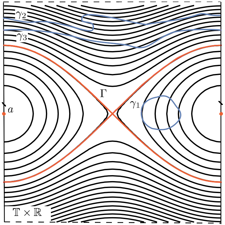
Figure 2: Sketch of the intersection of potentially invariant tori of (15) on a Poincaré section of $M$, a cylinder formed by identifying the right and left edges, at fixed time. Here the singular leaves of $J$ on the section are $\Sigma=\{a\}\cup\Gamma$, where $\Gamma$ is the separatrix

The rotational tori $\gamma_{2}$ and $\gamma_{3}$ are not of null-homology in $\mathcal{M}$. However, $\gamma_{2}$ does not remain transverse to the foliation generated by $J$, and thus will contain dependent points. This situation can happen if the dynamics of (15) no longer satisfied a twist (or tilt) condition. Finally $\gamma_{3}$ is everywhere transverse to the foliation, and thus no orbit on this set will satisfy the converse KAM theorem.

III Examples

In this section, we describe two volume-preserving systems and derive several foliations generated from adiabatic invariants or approximate integrals. These systems will be tested against the converse KAM condition with respect to the generated foliations in §V.

III.1 Two-Wave Model

As a first example, we will follow the original work of MacKay Mac (89) and study the motion of a charged particle with momentum $p$ in the potential of two longitudinal electrostatic waves. Without loss of generality, we can choose one of the waves to have phase velocity zero and the other to have phase velocity one and normalize the mass of the particle to one ED (81). This model, of the form (15), can be described by a nonautonomous Hamiltonian system,

$$H(q,p,t)=\tfrac{1}{2}p^{2}-\mu\cos(2\pi q)-\mu\nu\cos(2\pi k(q-t)),\qquad\mu,\nu\in\mathbb{R},\,k\in\mathbb{N}.$$ (16)

Thus the first wave has amplitude $\mu$, and the second has amplitude $\mu\nu$ and wavenumber $k$. By considering $q\mod 1$ and $k(q-t)\mod 1$, the phase space can be thought of as $\mathbb{T}\times\mathbb{R}\times\mathbb{T}$.

In fact, using the Poincare-Liouville one-form (11) we see that the system is Cartan-Arnol’d, that is, the Hamiltonian vector field $v$ associated to (16) also satisfies $\iota_{v}\alpha=0$. Thus we can use the sign of $K$, (13), in our computations.

The Hamiltonian (16) is perhaps the simplest nonintegrable, nonlinear Hamiltonian with two resonant terms. There are two obvious integrable limits:

1. $\mu=0$ yields the Hamiltonian for the motion of a free particle,

   $$H(q,p,t)=\tfrac{1}{2}p^{2}.$$ (17)

2. $\nu=0$ yields the Hamiltonian for a standard pendulum,

   $$H(q,p,t)=\tfrac{1}{2}p^{2}-\mu\cos(2\pi q).$$ (18)

If either $\mu\ll 1,\nu\sim O(1)$ or $\nu\ll 1,\mu\sim O(1)$ the dynamics is “nearly integrable”, and thus, by KAM theory, there will be a large set of invariant two-tori.

Following Mac (89), we will study (16) with $\nu=k=1$. Poincaré sections for four values of $\mu$, are shown in Fig. 3. Note that since the system is periodic in $t$, the section can be taken at $t=0\mod 1$. Near $\mu=0$, most orbits lie on rotational invariant tori, but as $\mu$ increases, the section exhibits two primary elliptic fixed points near $(0,0)$ and $(0,1)$ and two hyperbolic fixed points near $(\tfrac{1}{2},0),(\tfrac{1}{2},1)$. The figures only show the lower wave, near $p=0$. Of course, these fixed points correspond to elliptic and hyperbolic periodic orbits of the nonautonomous flow. The tori encircling the primary elliptic orbits are librational; they correspond to particles trapped in one of the two electrostatic waves.

(a) $\mu=0.0075$

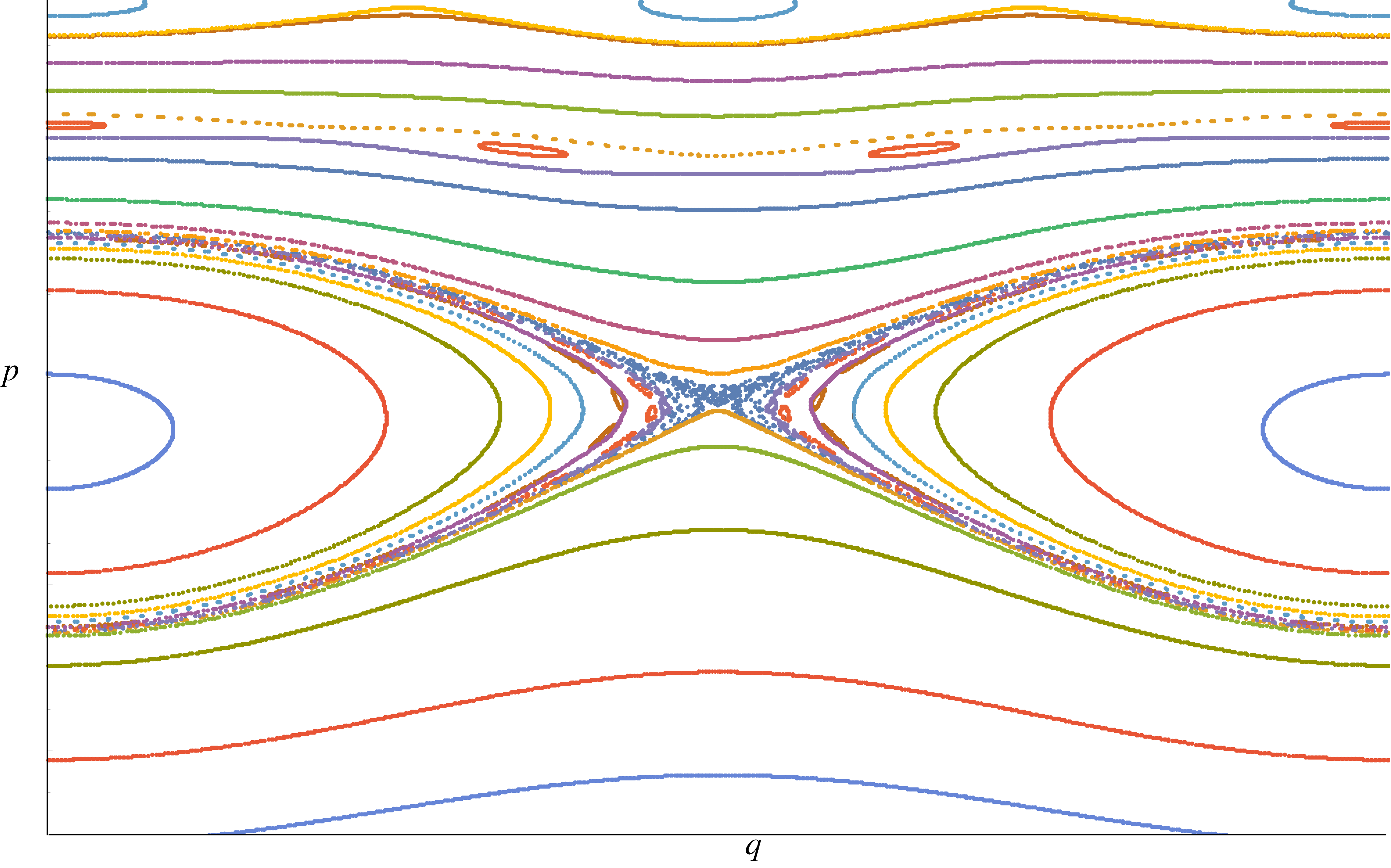
(b) $\mu=0.015$

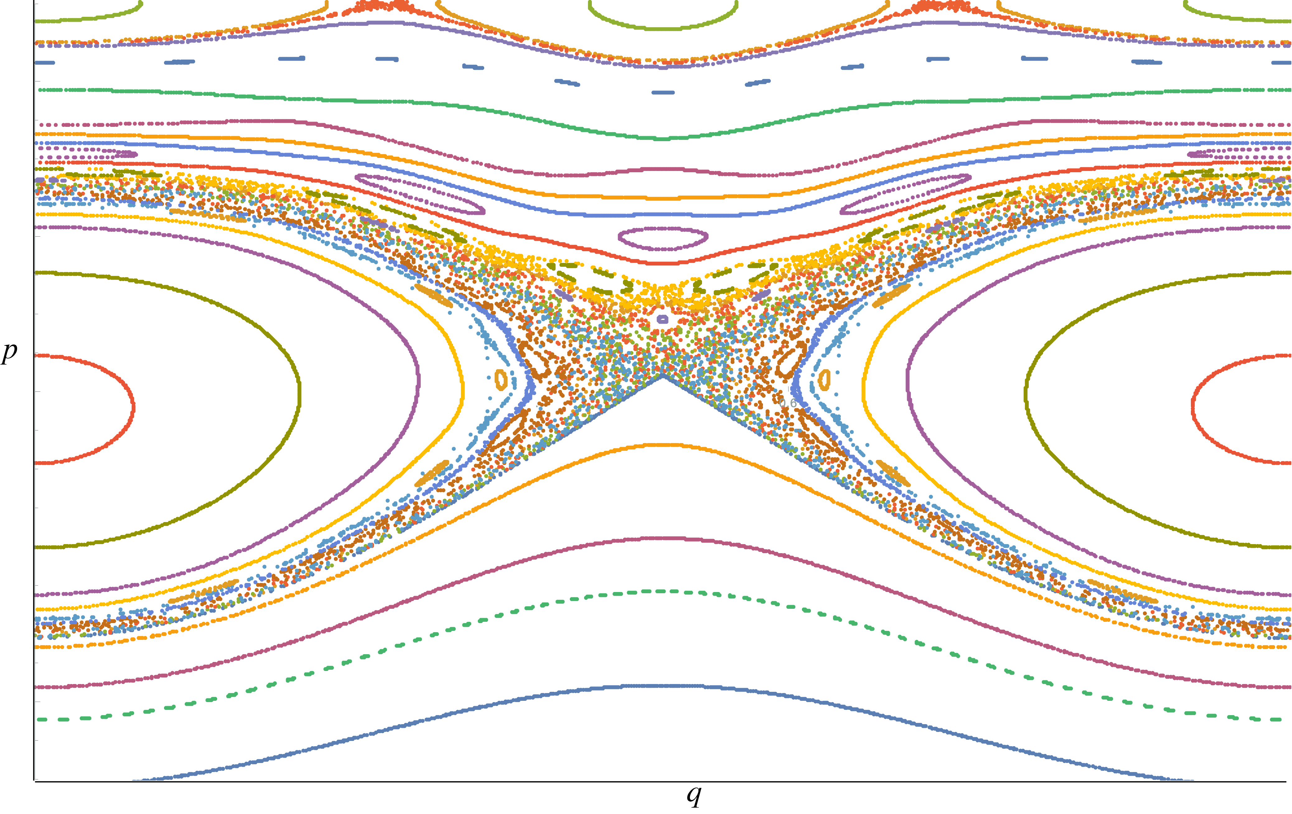
(c) $\mu=0.0225$

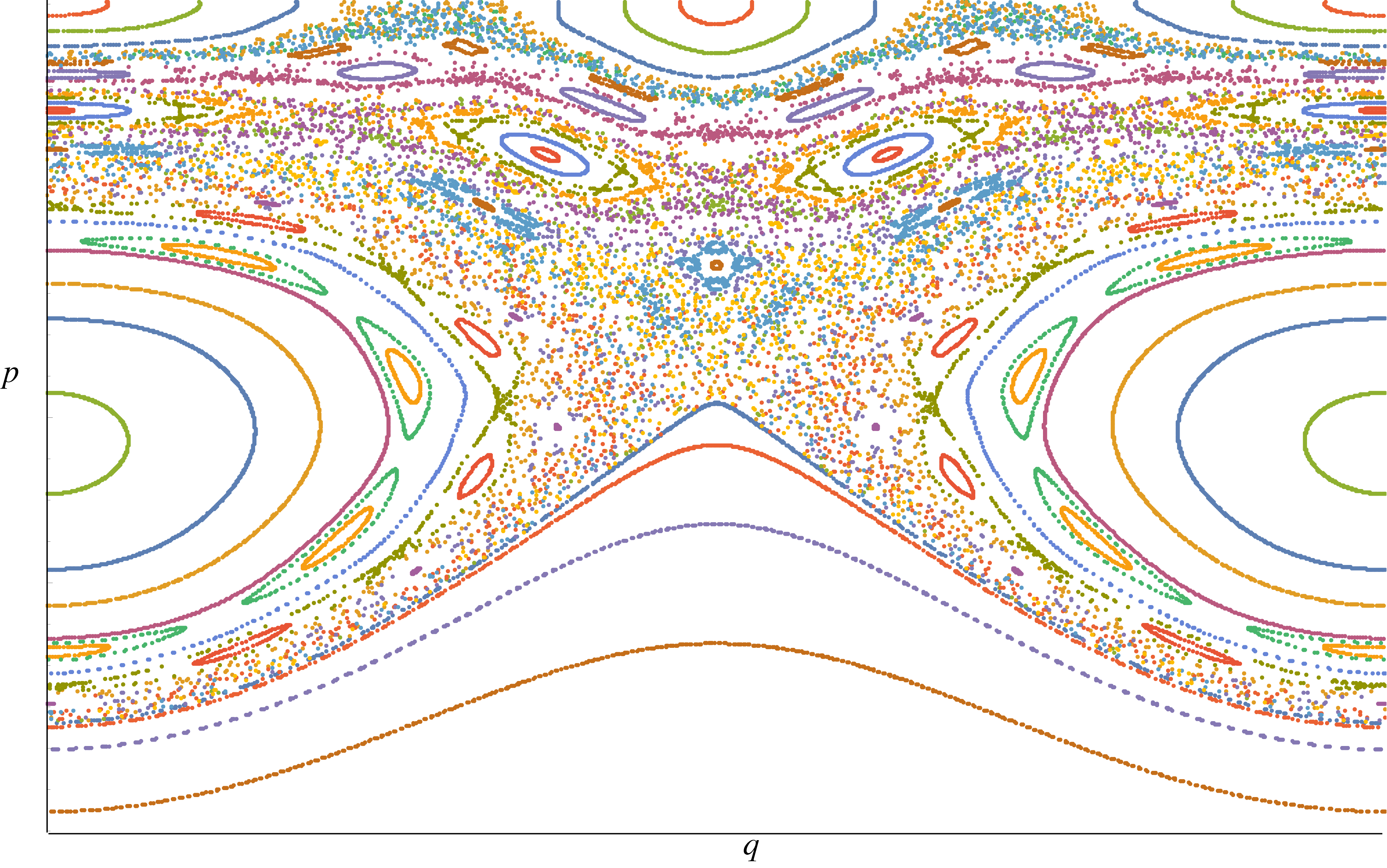
(d) $\mu=0.03$

Figure 3: Poincaré sections for (16) at $t=0$ for four values of $\mu$ when $\nu=k=1$. The domain of the figures is $(0,1)\times(-\frac{1}{2},\tfrac{1}{2})$.

By $\mu=0.015$, chaos is clearly evident near $(\tfrac{1}{2},0)$ in Fig. 3(b). As $\mu$ increases a secondary island appears near $p=\tfrac{1}{2}$ that generates its own chaotic region. As $\mu$ increases further, more resonant rotational tori break up, creating island chains and chaos near their hyperbolic orbits. This is clearly evident in Fig. 3(c). By $\mu=0.03$, in Fig. 3(d), the chaotic region around the secondary island merges with that of the original island: Chirikov’s resonance overlap.

Converse KAM theory was applied to this model in Mac (89). MacKay looked for orbits that do not lie on rotational invariant tori and gave several related “criteria” for the existence of these tori. The most relevant to numerical application relies on finding conjugate points. When $H$ has positive definite kinetic energy, this criterion is equivalent to the foliation condition of Mac (18) upon choosing a foliation $\mathcal{F}$ that is the union of vertical lines:

$$\mathcal{F}=\bigcup_{(q_{0},t_{0})\in\mathbb{T}^{2}}\{(p,q_{0},t_{0}):p\in\mathbb{R}\}.$$

Of course this can also be thought of as the foliation generated by the function $J=\tfrac{1}{2}p^{2}$.

Below, we will extend MacKay’s results by choosing several different foliations. Our aim is to to capture some of the librational tori around the main resonances at $p=0$ and $1$, as well as those in the driven resonance near $p=\tfrac{1}{2}$.

III.2 Zaslavsky’s Q-Flows: A Beltrami Example

In this section, to contrast the results of the two-wave model, we will study Zaslavsky’s so-called Q-flows Zas (91). While these dynamical systems are similar to $1\tfrac{1}{2}$ degree-of-freedom Hamiltonian systems, they do not have an obvious global Poincaré section. We will argue that they are more properly thought of as vector fields obtained from a Cartan-Arnol’d one form.

We begin with a vector field $v_{0}=\hat{z}\times\nabla\psi_{q}=(-\partial_{y}\psi_{q},\partial_{x}\psi_{q},0)$, where the stream function is

$$\psi_{q}(x,y):=\sum_{j=1}^{q}\cos\left(x\cos(2\pi j/q)+y\sin(2\pi j/q)\right).$$ (19)

Note that $\psi_{q}$ is an invariant of the flow of $v_{0}$ since

$$v_{0}\cdot\nabla\psi_{q}=0.$$

Thus the orbits lie on the surfaces $\psi_{q}=const$. These stream functions have discrete, $q$-fold rotational symmetry on $\mathbb{R}^{2}$. For $q=1,2,3,4,6$, the contours of $\psi_{q}$ form a periodic lattice; otherwise they have quasi-crystal symmetry, see Fig. 4.

      

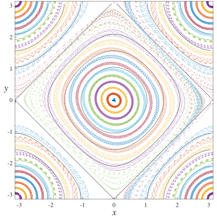
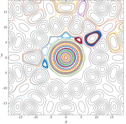
Figure 4: Projections of the flow of (20) onto the $(x,y)$ plane for $q=4$ (left), $q=5$ (right) and $\varepsilon=0.15$ for 25 initial conditions along the line $y=x$ for $z=0$. The contours of $\psi$ are shown as thin black curves. For $q=4$, periodicity is used in the $(x,y)$ plane.

The Q-flows correspond to a 3D perturbation of $v_{0}$, with the vector field

$$v=(\partial_{y}\psi_{q}+\varepsilon\sin(z),-\partial_{x}\psi_{q}+\varepsilon\cos(z),\psi_{q})$$ (20)

for each $\varepsilon\in\mathbb{R}$. This vector field maintains the $q$-fold symmetry about the $z$-axis. The case $q=4$ is a special case of the ABC vector field of DFG⁺ (86).

The vector field (20) is incompressible and satisfies the Beltrami condition:

$$\nabla\cdot v=0,\qquad\nabla\times v=\kappa v,$$ (21)

with $\kappa=1$, because $\nabla^{2}\psi_{q}=-\psi_{q}$,

Zaslavsky Zas (91) shows that the Q-flows can be formally thought of as a Hamiltonian system if one uses $z$ as an effective time variable. Unfortunately, this gives a singular vector field on the surfaces $\psi=0$. It is more appropriate to interpret $v$ as a Cartan-Arnol’d vector field using the form

$$\alpha_{q}=\left(\int^{y}\psi_{q}dy\right)dx-H(x,y,z)dz,$$ (22)

with the effective Hamiltonian

$$H(x,y,z)=\psi_{q}(x,y)+\varepsilon(y\sin(z)-x\cos(z)).$$ (23)

For this case the volume form (12) is $dy\wedge dx\wedge dz$ and the vector field $v$ is the unique vector field satisfying

$$\iota_{v}(dy\wedge dx\wedge dz)=d\alpha_{q}=\psi_{q}dy\wedge dx-dH\wedge dz,$$

Thus $\iota_{v}d\alpha_{q}=0$, and the form $\alpha_{q}$ generates the vector field $v$, up to a scalar scaling.

We will study in more detail the cases $q=4$ and $q=5$ as representatives of spatially periodic and quasi-periodic flows, respectively. When $\varepsilon=0$ and $q=4$, the $(x,y)$ phase portrait contains a square lattice of elliptic equilibria surrounded by a lattice of hyperbolic equilibria. Note that $\psi_{4}(x,y)=0$ on the hyperbolic points and their heteroclinic orbits so $z(t)$ is constant. For the case $q=5$, the contours of $\psi_{5}$ are a quasi-lattice (the contours in Fig. 4(b)), but there is still an elliptic orbit at the origin surrounded by a set of invariant tori. When $\varepsilon$ grows from zero, an increasing degree of chaos in the near the separatrices of these lattices is observed. Projections of the dynamics for $\varepsilon=0.15$ onto the $(x,y)$ plane are shown in Fig. 4.

When chaotic orbits of the Q-flows are unbounded they typically exhibit anomalous diffusion—that is, orbits travel along the channels associated with heteroclinic orbits, escaping from any bounded domain. The mean square drift grows with some non-integer power of $t$. This phenomenon is the motivation for the work in Zas (91). Here, we are more concerned with the breakup of tori, changes in topology, and birth of chaos as $\varepsilon$ increases. As we discuss next, to apply the converse KAM method we must start by constructing adequate foliations to detect these phenomenon.

IV Foliations

The primary aim of this section is to describe the various foliations to numerically test Thm. II.4 and determine the nonexistence of invariant tori transverse to these foliations.

IV.1 Two-Wave Model

For the two-wave model (16), five foliations are considered, each of which is generated from the gradient flow of an integrable Hamiltonian.

1. r-foliation: Generated from the gradient flow of the free particle Hamiltonian (17). It is designed to capture so called rotational tori. Specifically, it is the foliation given by

   $$\mathcal{F}^{r}=\bigcup_{q_{0},t_{0}}\{(p,q_{0},t_{0})|p\in\mathbb{R}\}.$$ (24)

2. l-foliation: Generated from the gradient flow of the harmonic oscillator Hamiltonian $H=\tfrac{1}{2}(p^{2}+q^{2})$. It is designed to capture the so called librational tori around the elliptic fixed point $(0,0)$ of the Poincaré section. This foliation is given by rays of constant angle from the origin in the $(q,p)$ plane:

   $$\mathcal{F}^{l}=\bigcup_{\theta,t_{0}}\{(r\cos\theta,r\sin\theta,t_{0})|r\in\mathbb{R}^{+}\}$$ (25)

   Note that this foliation is singular along $(q,p)=(0,0)$. Consequently, the curve $(q,p)=(0,0)$ needs to be removed from the phase space. Any orbit that intersects this removed curve is removed from consideration of the converse KAM theorem.

3. p-foliation: Generated from the gradient flow of the pendulum Hamiltonian (18). It is designed to capture both rotational and librational tori. This foliation $\mathcal{F}^{p}_{\mu}$ changes with the value of $\mu$, and is thus technically a family of foliations. This foliation reduces to $\mathcal{F}^{r}$ when $\mu=0$.

   As in the l-foliation, the p-foliation has singular points. These occur along $(q,p)=(0,0)$ and $(q,p)=(\tfrac{1}{2},0)$, and are elliptic and hyperbolic, respectively. Any orbit that passes though either of these singularities must be removed from consideration under the converse KAM theorem.

4. s1-foliation: Generated by the gradient flow of a first order global invariant,

   $$J=\tilde{H}_{\mu}(q,p,t)=-\tfrac{1}{2}p^{2}+\tfrac{1}{3}p^{3}-\mu\left[(p-1)\cos(2\pi q)+\nu p\cos(2\pi k(q-t))\right].$$ (26)

   Taking the orbits of the gradient flow of (26) for each value of $\mu$ gives the family of foliations $\mathcal{F}^{s}_{\mu}$. The invariant is computed using a method called ‘global removal of resonances’ from LL (92). The details of this method and its application to the two-wave model are given in Appendix A.

   The foliations $\mathcal{F}^{s1}_{\mu}$ are designed to capture both rotational and librational tori around $(0,0)$, as well as librational tori about the elliptic fixed point $(0,1)$, and track the movement of the two elliptic fixed points starting at $(0,0)$ and $(0,1)$ as $\mu$ varies.

5. s2-foliation: Generated by the gradient flow of a second order global invariant, (38). It is designed to capture all features of the s1-foliation as well as librational tori arising from the $1:2$ resonance. The family of foliations is denoted by $\mathcal{F}^{s2}_{\mu}$. The invariant (38) is computed using a higher order method of the global removal of resonances from LL (92). This higher order method was first realized in McN (78) and its details and application to the two-wave model are given in Appendix A.

   The level sets of (38) at the slice $t=0$ are given in Figure 5.

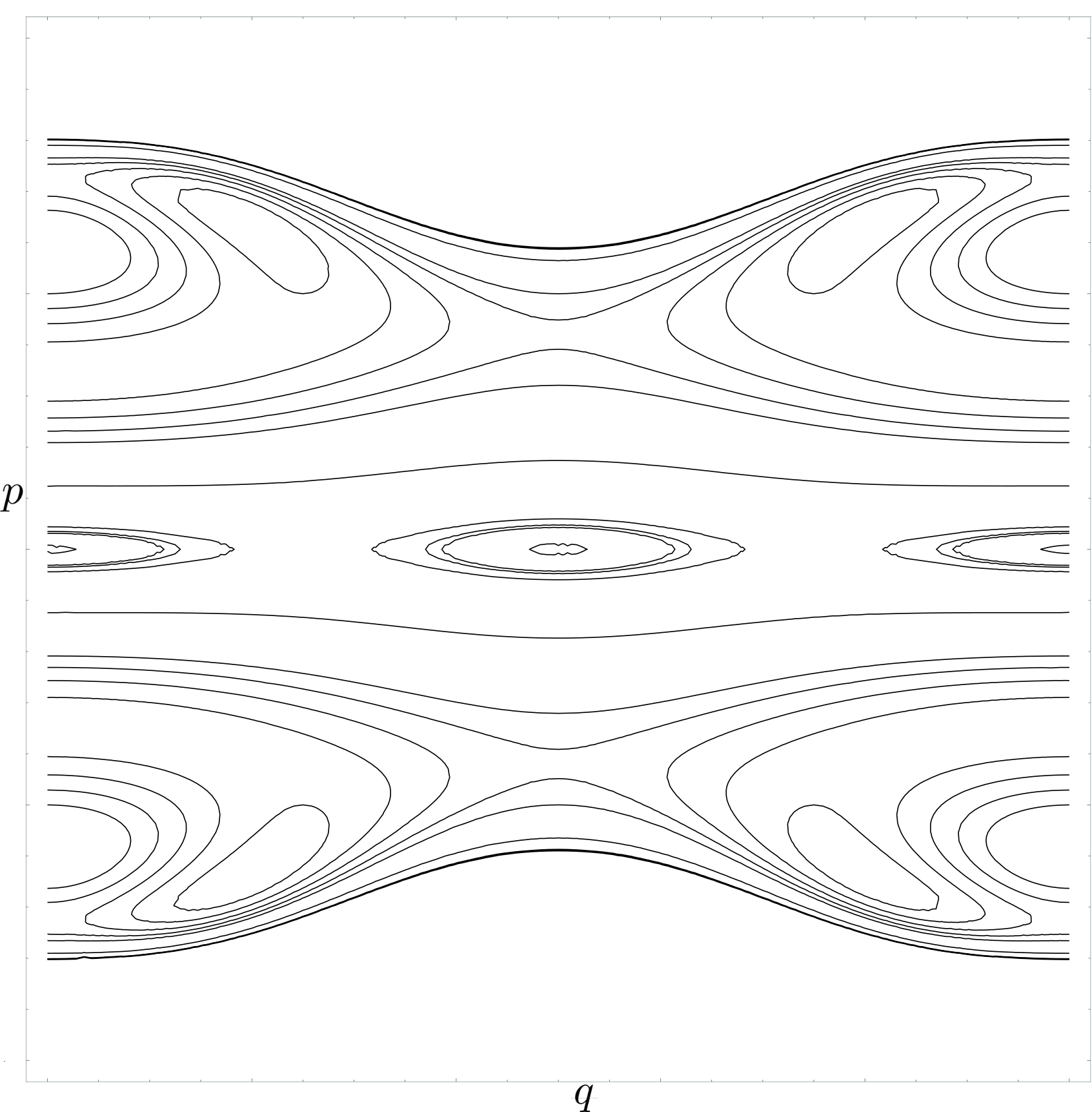
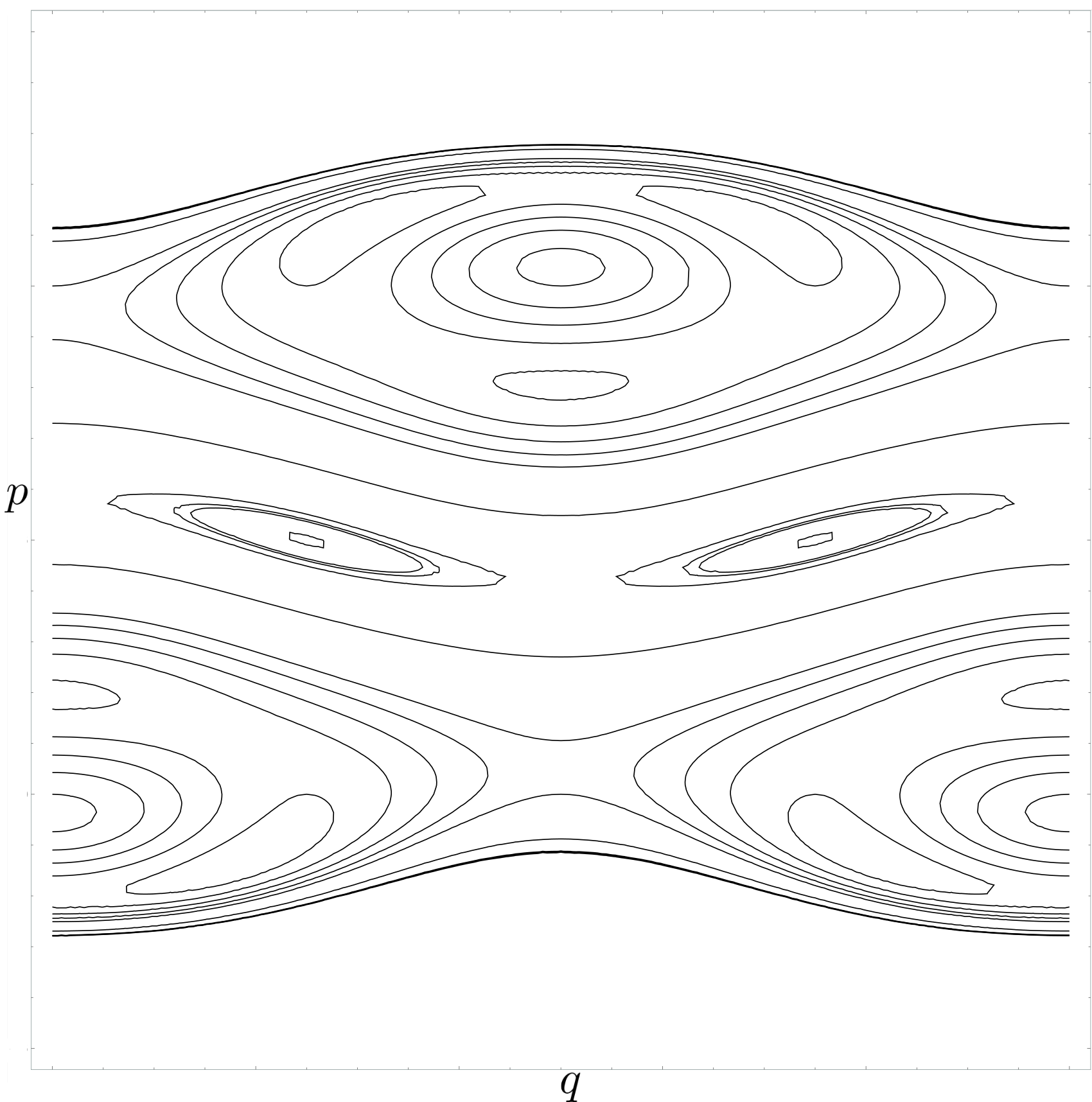
Figure 5: Level sets for the foliation $\mathcal{F}^{s2}_{0.02}$ at time $t=0$ (left) and $t=\tfrac{1}{2}$ (right). The domain of the figures is $(0,1)\times(-0.5,1.5)$.

IV.2 Q-Flow

For the Q-flows defined in (20) we will consider only two foliations:

1. l-foliation: Generated from the gradient flow of the Hamiltonian for the harmonic oscillator $H(x,y,z)=\tfrac{1}{2}(x^{2}+y^{2})$. The foliation is expected to capture only the primary librational tori that continue from those that encircle the elliptic orbit at $(0,0)$ for $\varepsilon=0$.

2. $\psi$-foliation: Generated from gradient flow of the approximate invariant $\psi_{q}(x,y)$ (19). This foliation should capture the librational tori around any elliptic point in the periodic or quasi-periodic lattice of $\psi_{q}$.

V Results

In this section we will compute the converse KAM condition for the two-wave and Q-flow models. In each case we will use several foliations, as discussed in §IV. The main results are shown below in Figs. 7, 8, 9, 10, 12, 15 and 17.

V.1 Numerical Implementation

For each model and each foliation the condition of Thm. II.4 will be tested numerically. Since both models can be formulated as Cartan-Arnol’d systems, we will use the techniques in §II.2. Thus the converse KAM condition is satisfied for the two-wave or Q-flow models only if,

$$K_{tw}(t):=d\alpha(\xi_{t},\eta_{t}),\quad\mbox{or}\quad K_{qf}(t):=d\alpha_{q}(\xi_{t},\eta_{t}),$$ (27)

changes sign, respectively.

To compute the sign change we choose a proposed point $u_{0}\in M$ to check for nonexistence of an invariant surface, and numerically find the flow $\phi_{t}(u_{0})$. Since each foliation is determined by a function $J$, we choose

$$\eta_{t}=\nabla J(\phi_{t}(u_{0})),\qquad\xi_{0}=\eta_{0}=\nabla J(u_{0}).$$ (28)

so that $\eta_{t}$ is in the tangent space to the foliation at each point and $\xi_{0}$ begins parallel to $\eta_{0}$. The vector $\xi_{t}$ is then obtained by integration of the linearized equations (LABEL:eq:linearlization) about the orbit $\phi_{t}(u_{0})$.

As discussed in §II.2, $K(t)$ changing sign is necessary but not sufficient to check the hypothesis of Thm. II.3 as it equally detects $\varphi_{t}$ crossing $\pi$. To remedy this, we will only check the change of sign of $K(t)$ when $\eta_{t}\cdot\xi_{t}<0$, using the Euclidean dot product, as this guarantees that $\theta_{t}<\pi/2$.

Both models and their tangent orbits, are integrated numerically using the $5/4$-Runge-Kutta scheme of Tsitouras Tsi (11); specifically we use the algorithm Tsit5() of the DifferentialEquations.jl library in Julia. A callback function is used to determine sign changes in $K(t)$ when $\eta_{t}\cdot\xi_{t}<0$, and linear interpolation to find a more accurate value of $t_{c}$, the time for which $K(t_{c})=0$.

V.2 Two-Wave Model

We computed the converse KAM condition for the two-wave model for the five different foliations $\mathcal{F}^{r}$, $\mathcal{F}^{l}$, $\mathcal{F}^{p}$, $\mathcal{F}^{s1}$ and $\mathcal{F}^{s2}$ defined in §IV.1. We typically chose a grid of $500$ values for $\mu\in[0,0.03]$, and of $500$ initial points on the line $(0,p_{0},0)$ for $p_{0}\in[0,1]$. For each initial point we integrated the orbit until either the converse KAM condition was satisfied at some time $t_{c}$ or $t$ reached time $150$.

However, first we address the choice of maximum integration time. The choice $t_{c}\leq 150$, seemed to be sufficient to capture most of the points that satisfy the converse KAM condition. This is indicated by Fig. 6, which shows a histogram of the number of points captured at time $t_{c}$ for the s1-foliation over the entire $500\times 500$ grid. It is evident that by $t=150$ the vast majority of points that would eventually satisfy the converse KAM criterion are captured. A similar convergence is also seen for the other foliations.

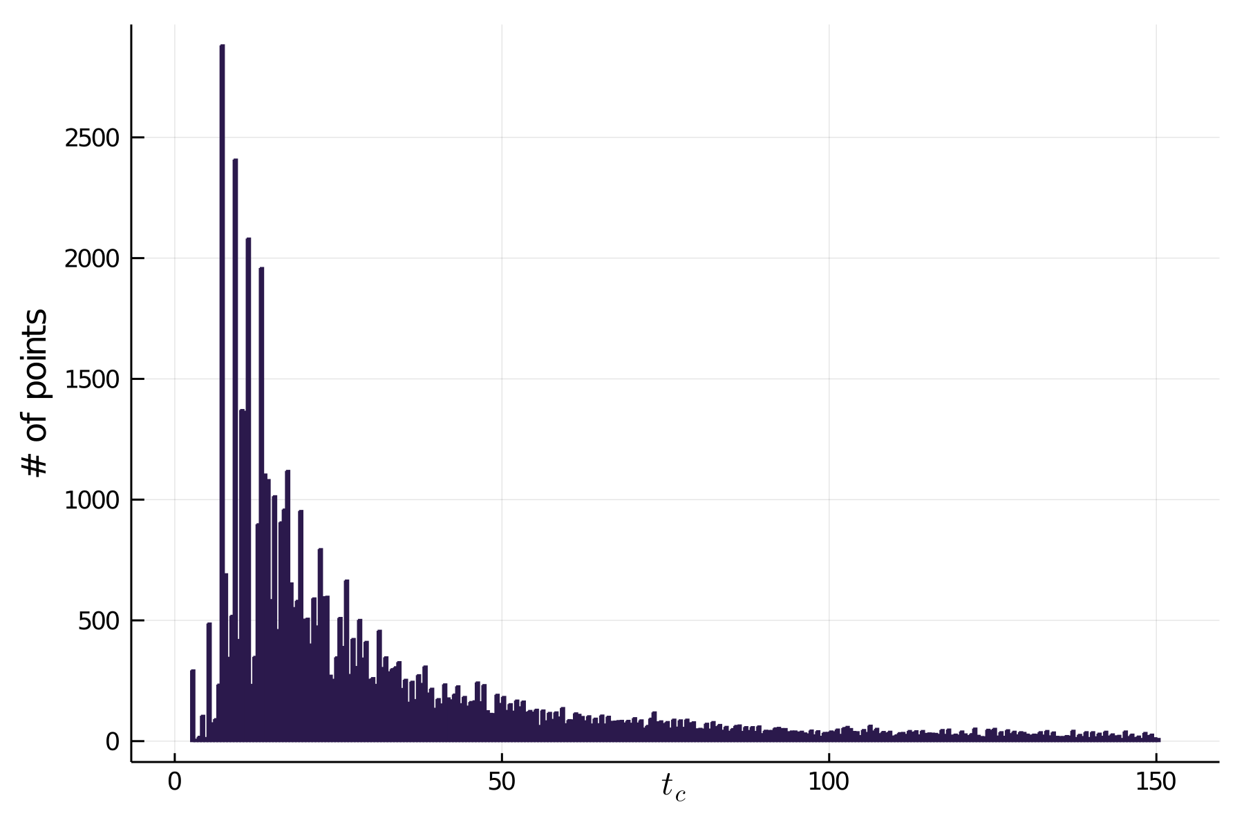
Figure 6: Histogram of the number orbits transverse to the s1-foliation at time $t_{c}$ for $250,000$ orbits of the two-wave model with $\mu\in[0,0.03]$.

The results of the computations are shown in Figs. 7, 8, 9, 10 and 12 for the five foliations. As we will argue below, the results for the various foliations differ, especially with respect to librational tori in various resonances of the dynamics.

The results for the r-foliation $\mathcal{F}^{r}$, are shown in Fig. 7. In the left panel, which is equivalent to Fig. 4 of Mac (89), each initial condition that satisfies the converse KAM condition, i.e., that does not lie on an invariant surface transverse to the foliation, is colored blue, and the darker hues indicate a smaller value of $t_{c}$.

In the right panel of Fig. 7, we show the $t=0$ Poincaré section for each of the orbits that pass the converse KAM condition for $\mu=0.015$. The contours of the foliation are also overlaid on the panel. Note that any initial conditions that lie within the 0:1 and 1:1 resonance islands do not lie on invariant surfaces transverse to the r-foliation and thus they pass the converse KAM condition “dependently”. These correspond to librational tori around the two primary elliptic orbits that start near $(q,p,t)=(0,0,0)$ and $(0,1,0)$. This is expected; clearly librational tori, whose Poincaré sections are circles about their respective elliptic points, fail to be transverse to planes of constant $p$. This explains the two dark blue regions in the left panel that grow in width as $2\sqrt{\mu}$, the half-width of these islands. Also seen in this panel are several tongues, the largest of which has a width that grows linearly in $\mu$ starting near $(\mu,p_{0})\approx(0.002,0.5)$. This corresponds to the driven resonance near $p=\tfrac{1}{2}$ that was seen in Fig. 3 and is clearly visible in the right panel of Fig. 7 as well.

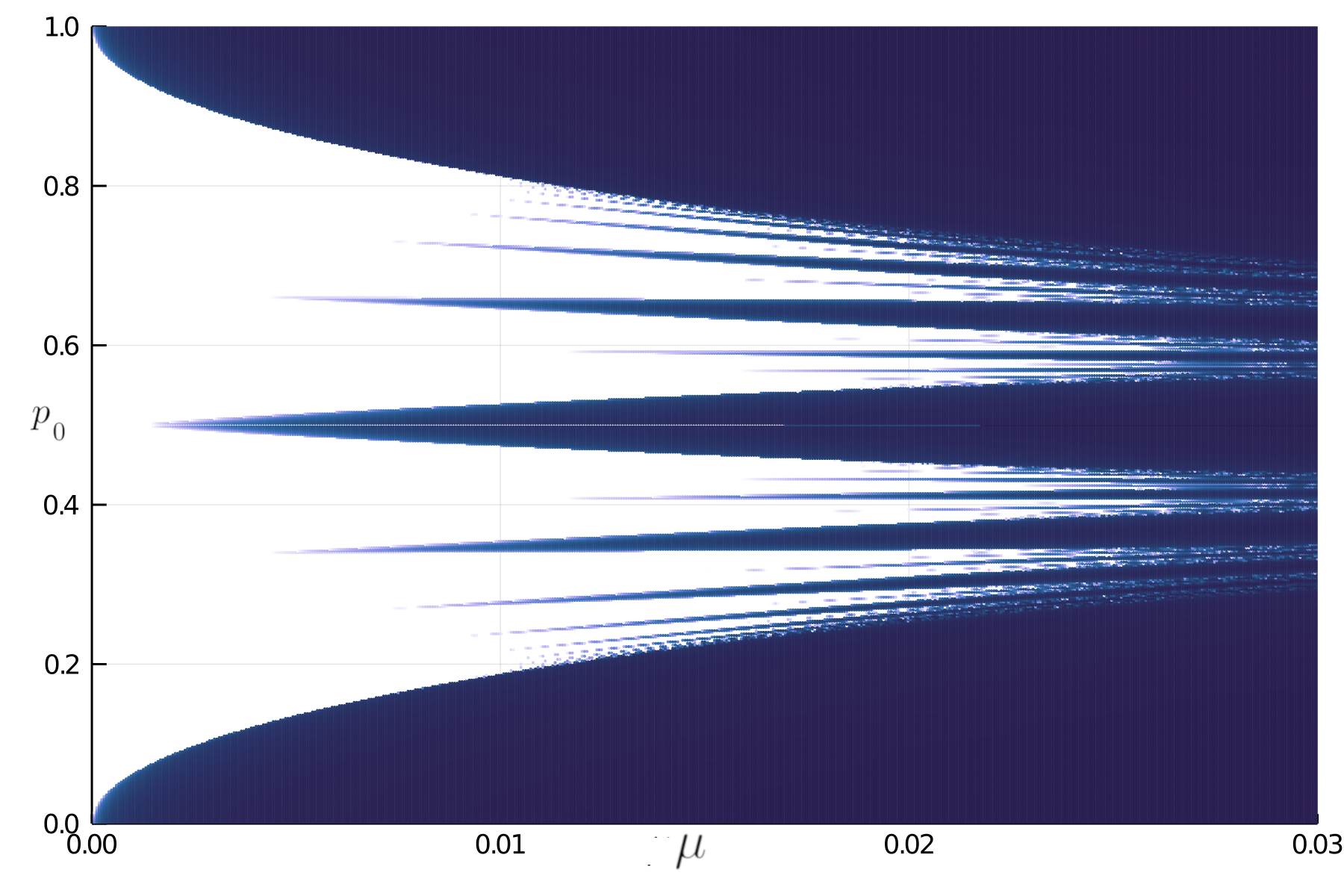
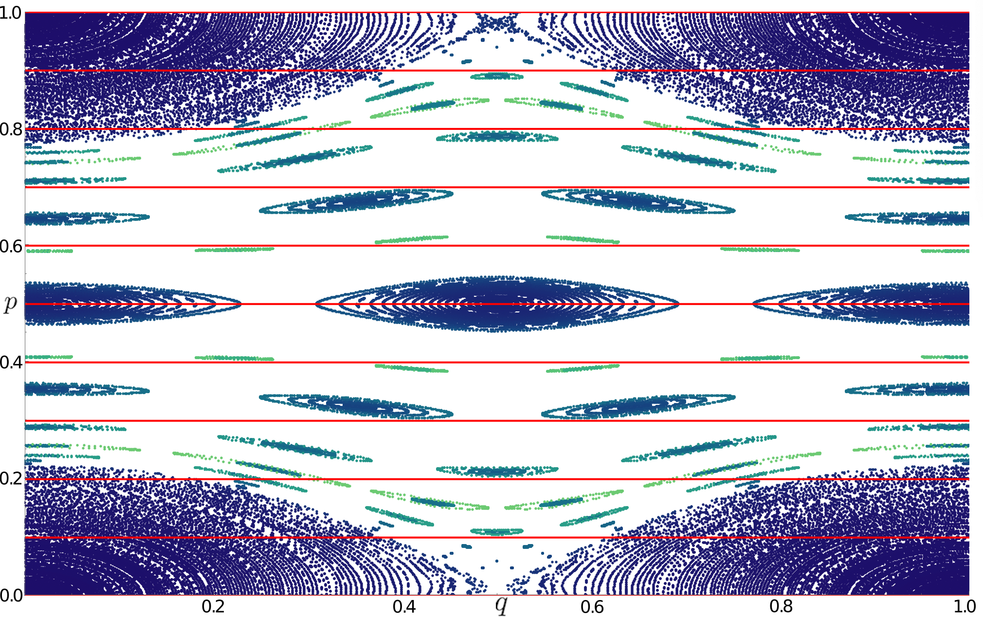
Figure 7: (r-foliation) (a) The left panel depicts the values of $(\mu,p_{0})\in[0,0.03]\times[0,1]$ that pass the converse KAM condition within the time $t_{c}\leq 150$ for the r-foliation. The points are colored according to the time taken to transversality violation, with a darker blue indicating a shorter time. (b) The right panel shows a $t=0$ Poincaré section of the orbits from (a) for $\mu=0.015$. The red curves are a cross-section of the level sets of the generating invariant for the foliation, namely $p^{2}$.

The l and p-foliations are shown in Figs. 8 and 9, respectively. For the range $0.2<p_{0}<1.0$, these figures share many features of the r-foliation. However, the librational tori near $(q,p,t)=(0,0,0)$ no longer satisfy the converse KAM condition, that is, the computations correctly indicate that these orbits lie on invariant tori. In addition, small spikes close to the curve $p_{0}=2\sqrt{\mu}$ are now evident; these represent the incursions of resonant islands into the edge of the main resonance. The p-foliation differs subtly from the l-foliation in that there are slight differences in some of the resonance tongues.

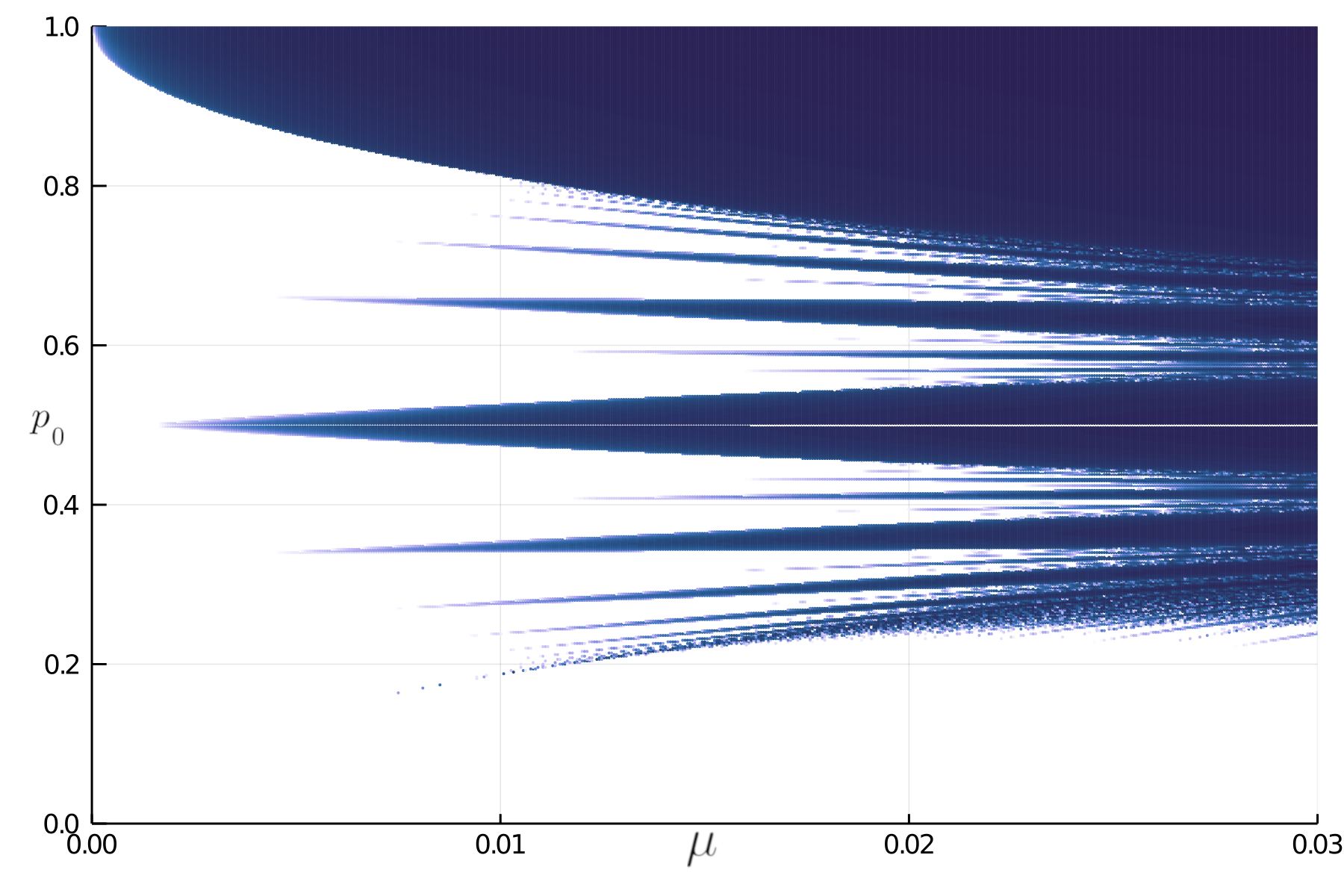
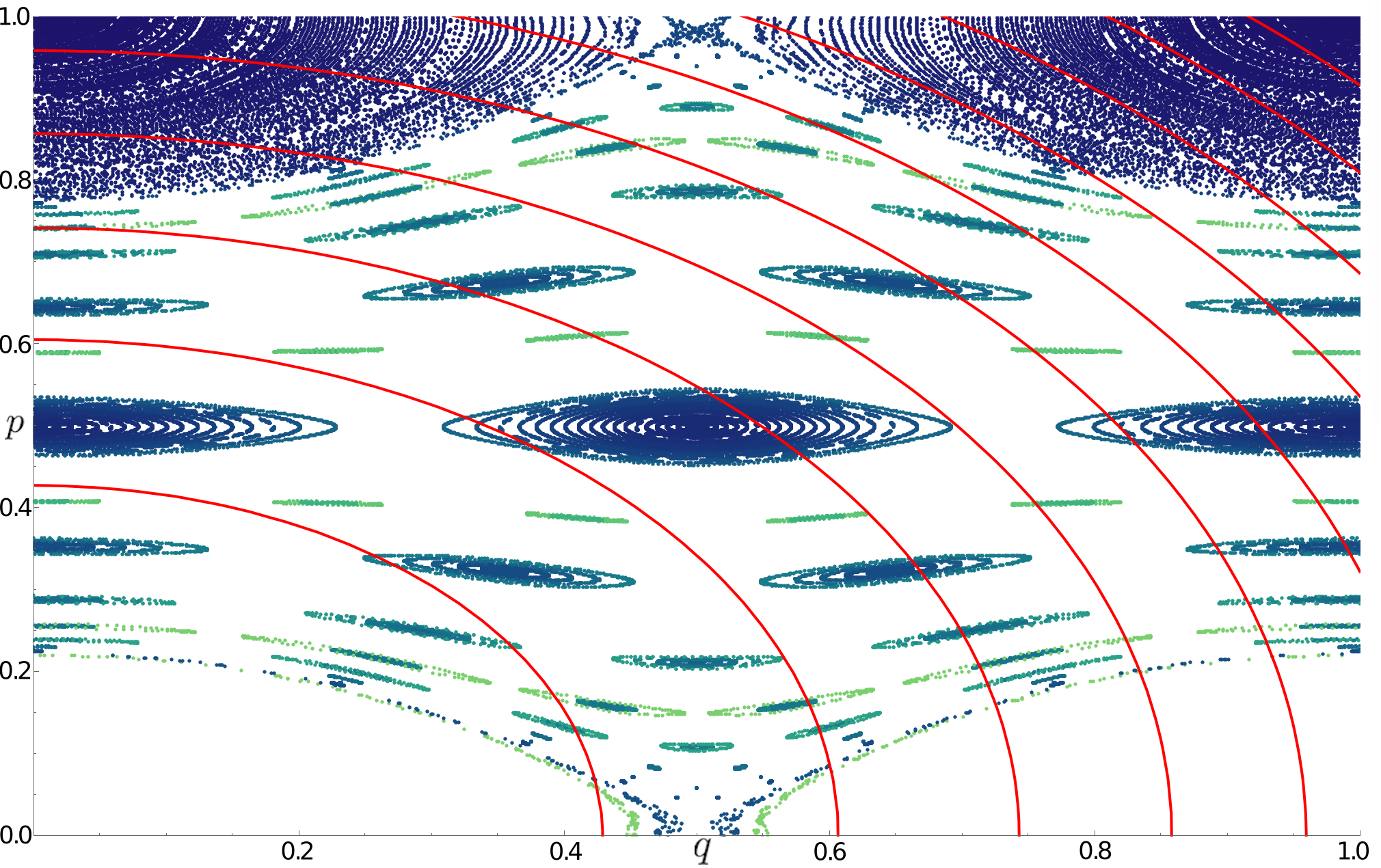
Figure 8: (l-foliation) Orbits satisfying the converse KAM condition for the l-foliation (details as in the caption to Fig. 7). The red curves (right panel) correspond to the Hamiltonian $\tfrac{1}{2}(p^{2}+q^{2})$.

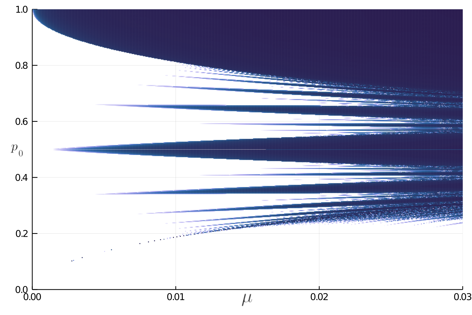
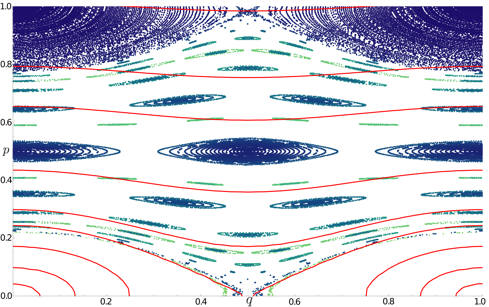
Figure 9: (p-foliation) Orbits satisfying the converse KAM condition for the p-foliation (details as in the caption to Fig. 7). The red curves (right panel) correspond to the Hamiltonian (18).

Though the s1-foliation, in Fig. 10, is nearly identical to the p-foliation for $0<p<0.8$, it also now identifies points on librational tori in the 1:1 resonance. Thus the s1-foliation correctly identifies the regular regions about both the $0:1$ and $1:1$ resonances.

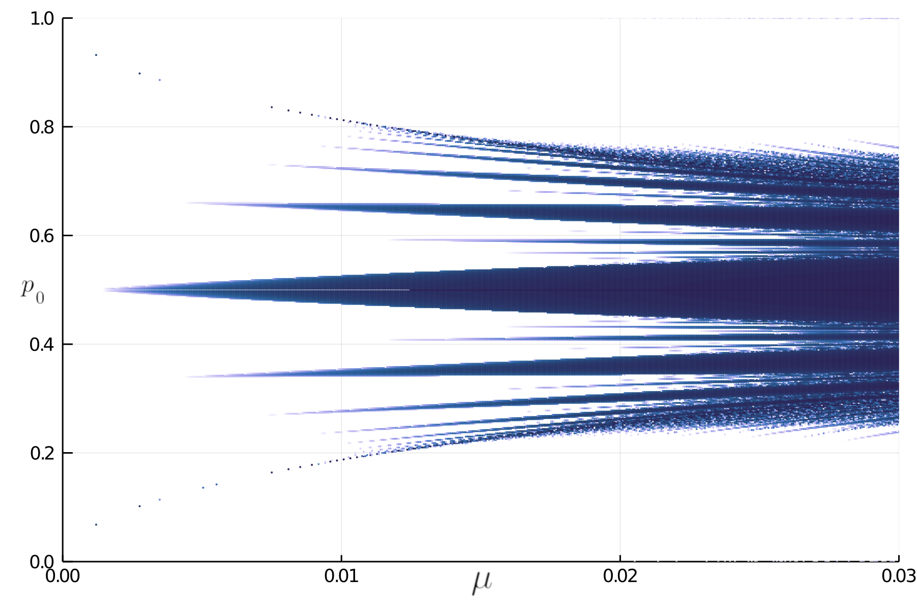
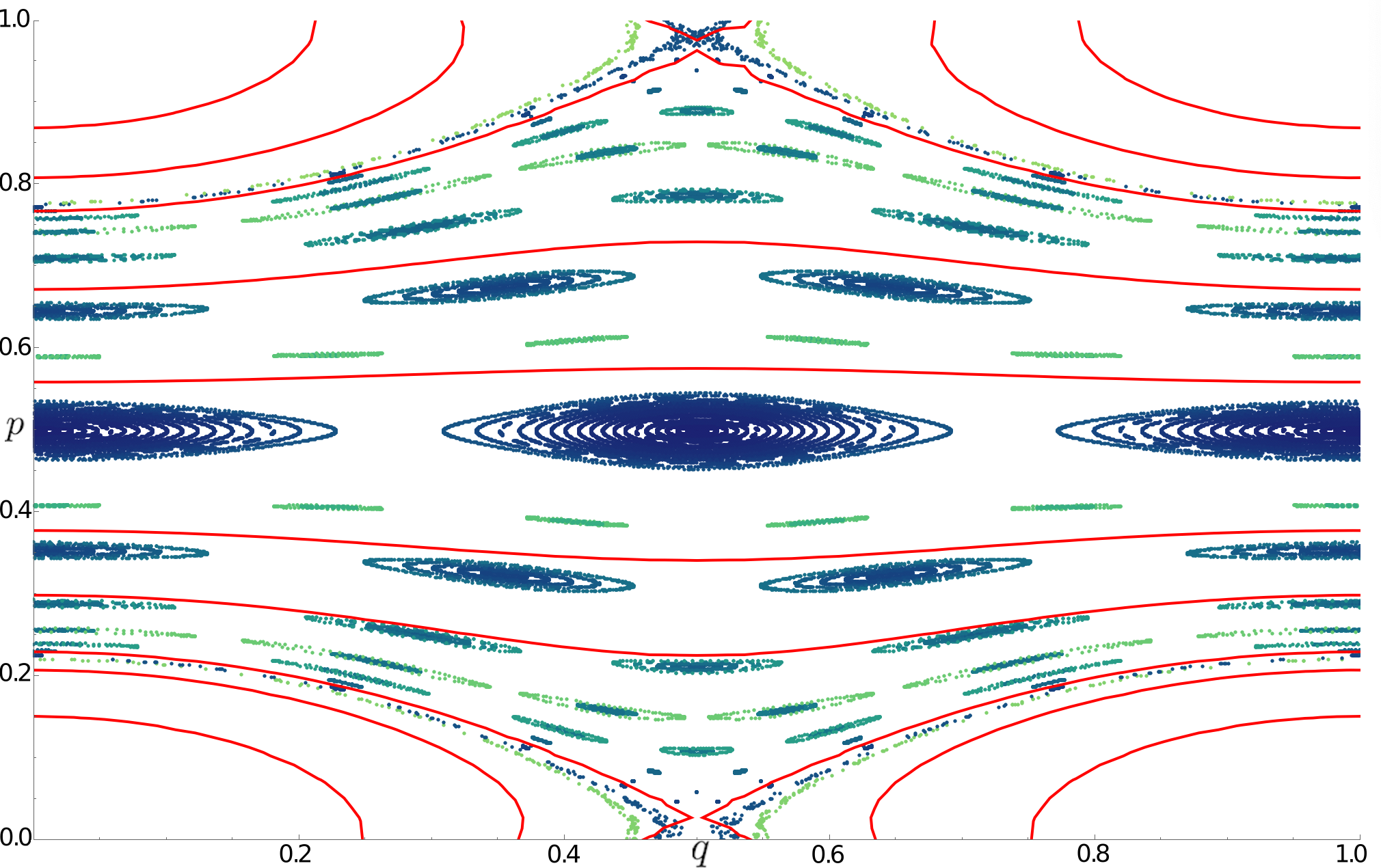
Figure 10: (s1-foliation) Orbits satisfying the converse KAM condition for the s1-foliation (details as in the caption to Fig. 7). The red curves (right panel) correspond to the Hamiltonian (26).

Two constant-$\mu$ slices though the results for the s1-foliation are shown in Fig. 11. These plots show the inverse of the time taken to pass the converse KAM condition $1/t_{c}$ as a function of $p_{0}$ $\mu=0.015$ (left panel) and $\mu=0.03$ (right panel). The peaks in each plot lie at the centre of the resonant tori not captured by the s1-foliation, or at the chaotic regions near the primary hyperbolic fixed point. These plots are analogous to those of Whi (15), who computed a rotation frequency for his phase vectors.

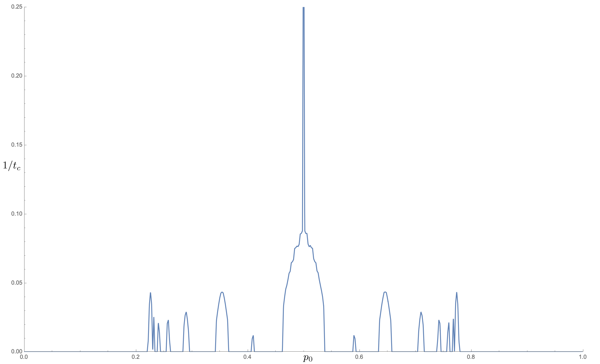
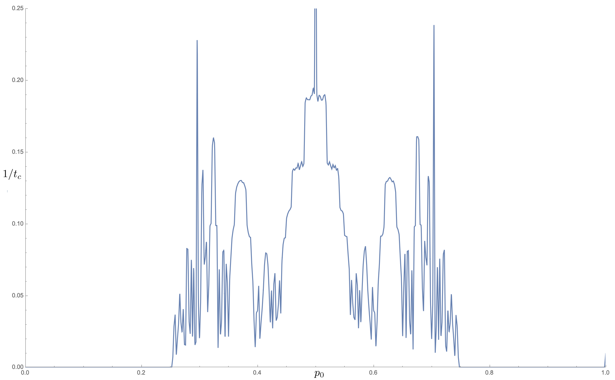
Figure 11: Plot of the inverse time $1/t_{c}$ taken to pass the converse KAM condition with respect to the s1-foliation for initial conditions $(0,p_{0})$ for (left) $\mu=0.015$ and (right) $\mu=0.03$.

Finally, Fig. 12 shows computations for the s2-foliation. This case is clearly different from the previous results for initial conditions in the 1:2 resonant island (near $p=\tfrac{1}{2}$). Indeed, as we saw in Fig. 5, this foliation has contours that are topologically similar to this island chain, and therefore many of these librational tori no longer satisfy the converse KAM criterion. Unfortunately, there are now regions that satisfy converse KAM near the 0:1 and 1:1 elliptic orbits, the blue regions near $p=0$ and $p=1$. These are apparently due to the fact that the contours of (38), shown in Fig. 5, have a large period three island trapped in the main resonances that is not present in the dynamics.

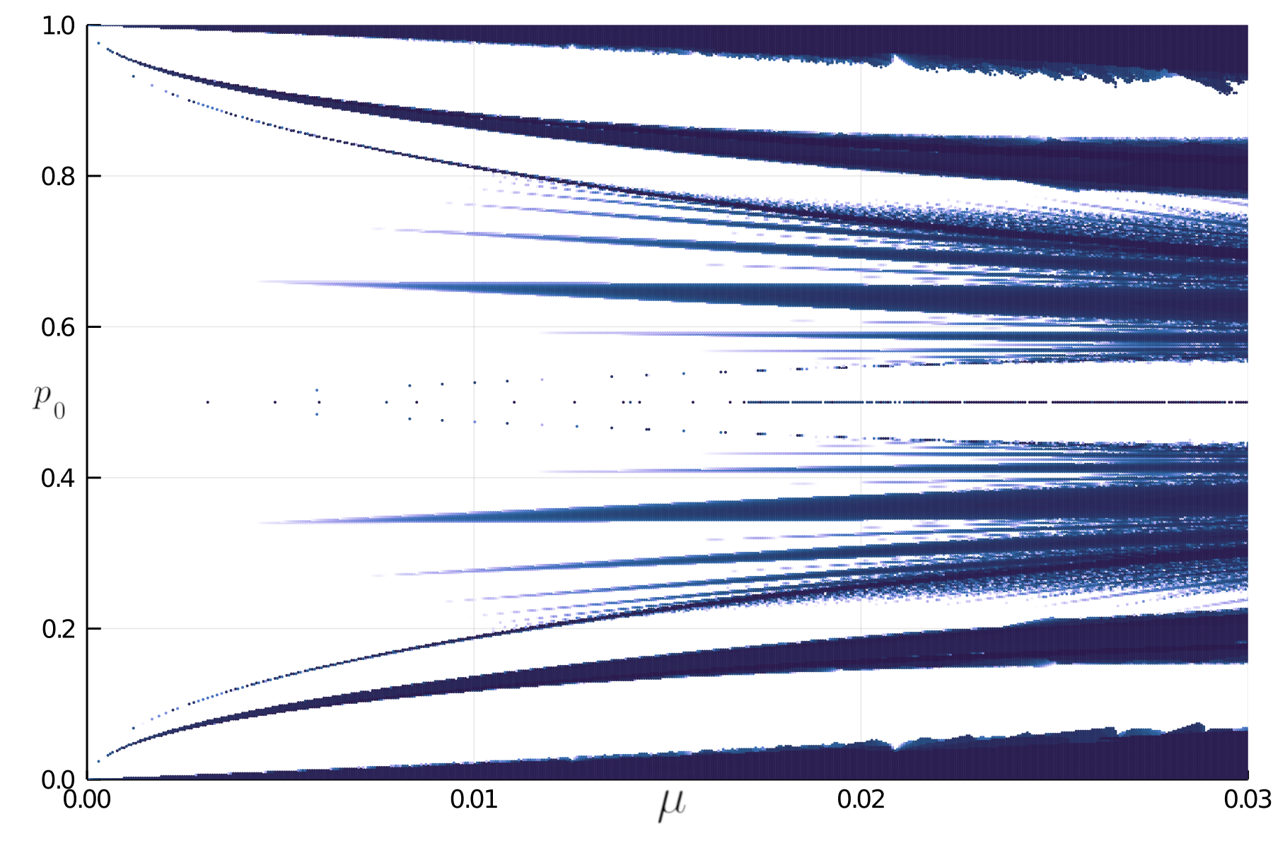
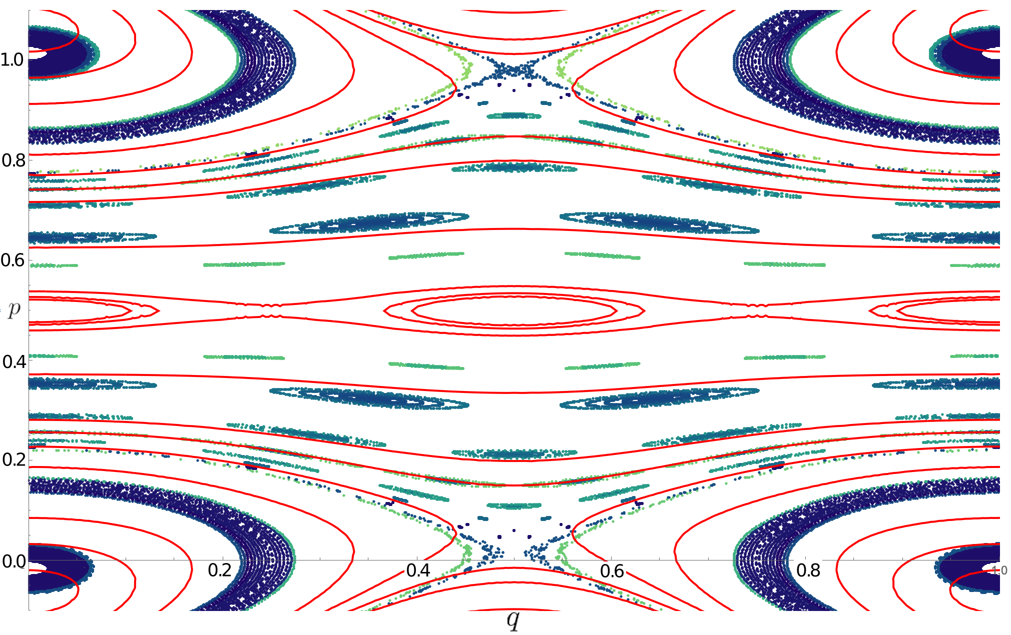
Figure 12: (s2-foliation) Orbits satisfying the converse KAM condition for the s1-foliation (details as in the caption to Fig. 7). The red curves (right panel) correspond to the Hamiltonian (38).

As a comparision, a computation of the finite time Lyapunov exponent is shown in Fig. 13. This shows the relative value of the computed Lyapunov exponent for each initial condition $(\mu,p_{0})$ integrated to $t=150$. Note that almost all of these exponents are quite small—those with $\lambda<0.05$ are colored white in the figure. However, it would be difficult to declare an orbit chaotic when $\lambda<0.2$ as it is for most of the parameters in the figure. Nevertheless, the domains where $\lambda>0.05$, correlate well with those that satisfy the converse KAM condition for the l and s1-foliations, apart from the regions in the interior of the 1:2 and higher-order resonances.

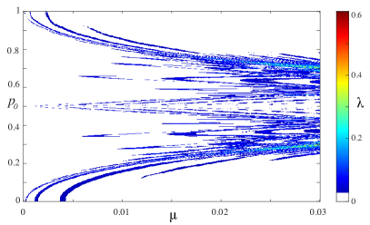
Figure 13: (Lyapunov Exponent) The finite time Lyapunov exponent for the same initial conditions as Figs. 7, 8, 9, 10 and 12.

To reveal the effect of the choice of section on the results, the converse KAM criterion with respect to the s1-foliation was tested on initial conditions $(q_{0},p_{0},0)$ for $q_{0}=0.25$ and $0.5$. The results are depicted in Fig. 14.

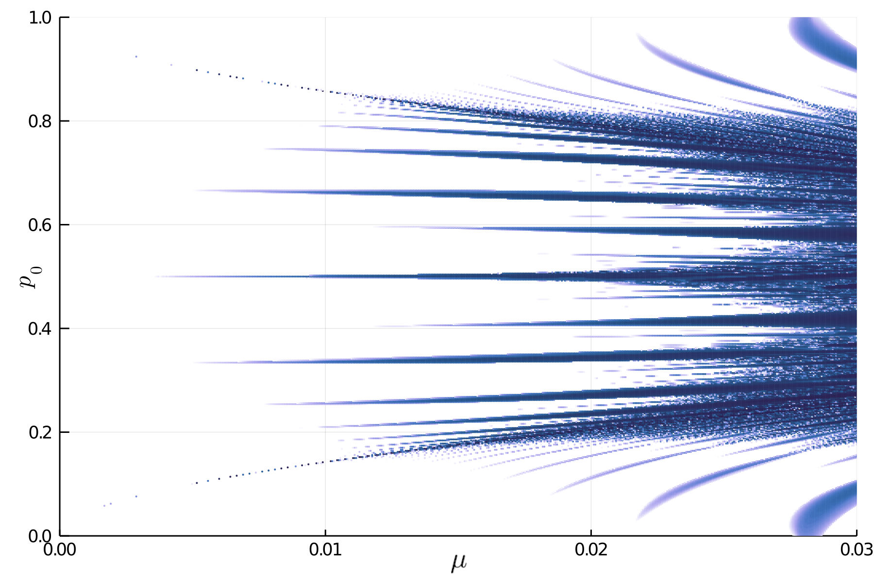
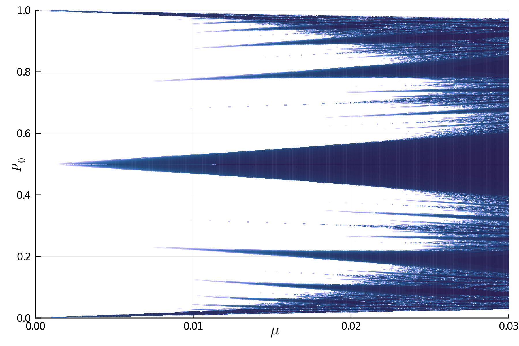
Figure 14: (s1-foliation) Points that pass the converse KAM condition for the s1-foliation for Poincaré sections at $t=0.25$ (left) and $t=0.5$ (right). Compare these to Fig. 10, which is on the section $t=0$.

V.3 Q-Flows

Computations of the converse KAM condition for the Q-flows, (20), are shown in Figs. 15 and 16 for $q=4$ and Figs. 17 and 18 for $q=5$. In each case, we choose $500$ initial conditions along a line in the phase space at $z=0$, and check the sign of $K_{qf}$ (27) for $t_{c}\leq 150$. As for the two-wave results, each point that satisfies the converse KAM condition is indicated in blue, and a darker blue indicates a smaller value of $t_{c}$.

For Fig. 15, the ordinate, $u_{0}$, represents initial conditions along the line $(x,y,z)=(u_{0},u_{0},0)$ and the abscissa is the perturbation strength, $\varepsilon$. Panels (a) and (b) compare the l-foliation to the $\psi$-foliation, respectively, for $(\varepsilon,u_{0})\in[0,0.5]\times[0,\pi]$. As was seen in Fig. 4(a), when $q=4$ the initial conditions with $u_{0}\in[0,\pi/2)$ correspond the lattice cell encircling the origin. For these initial conditions, the results of the two foliations are nearly identical. This can also be seen in panels (c) and (d), which display only orbits with $u_{0}\in[0,\pi/2]$ but extend the range of $\varepsilon$ to $[0,1]$. Both foliations correctly assess the expected growing chaotic zone that forms around the separatrix from the saddles at $(x,y)=(0,\pm\pi)$ and $(\pm\pi,0)$. They also indicate a narrow tongue near $u_{0}=1.2$ that starts near $\varepsilon=0.031$ in which there are no tori appropriate to the radial foliations.

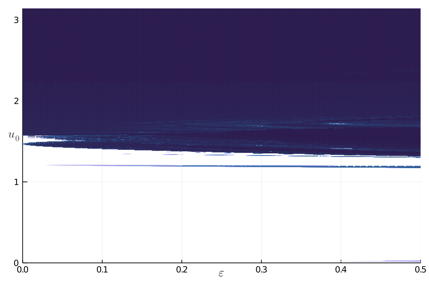
(a) l-foliation, $(\varepsilon,u_{0})\in[0,0.5]\times[0,\pi]$

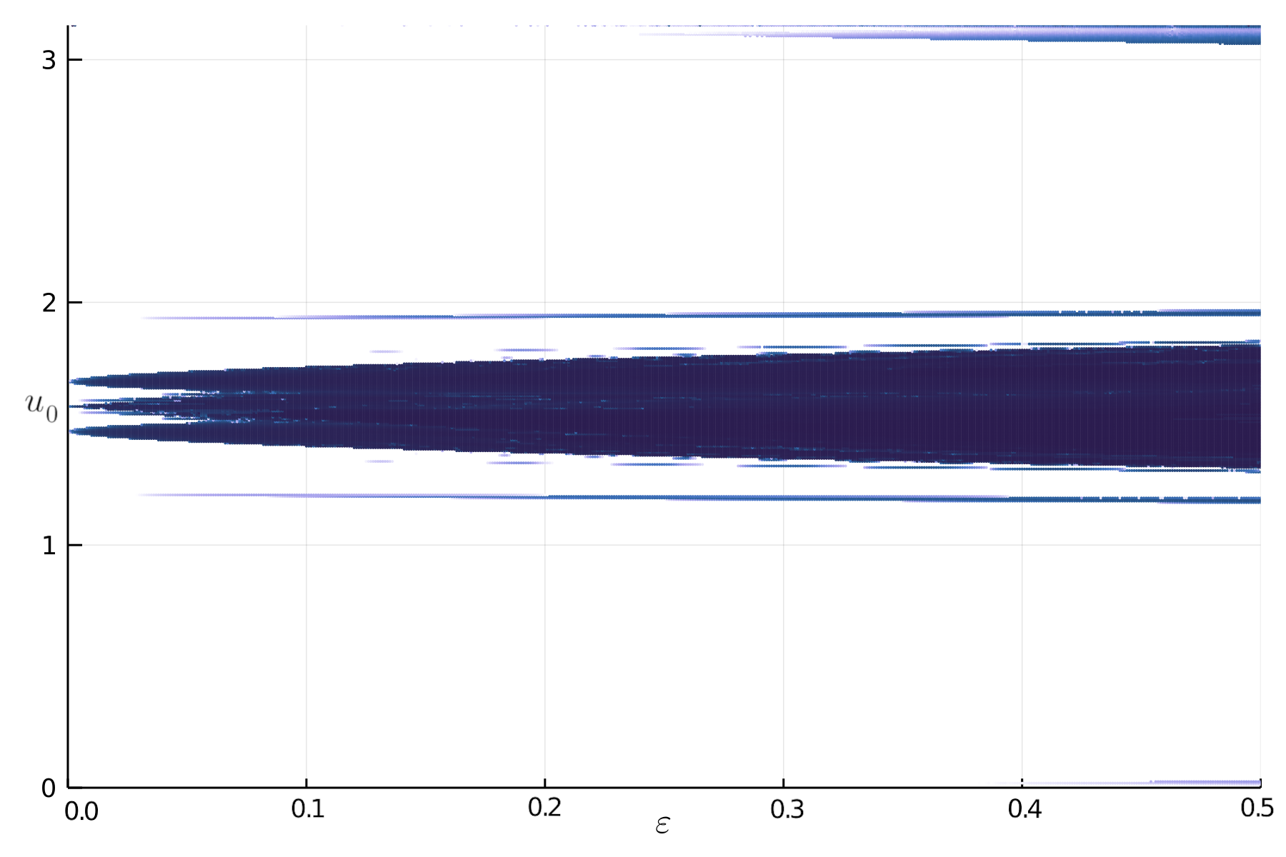
(b) $\psi$-foliation, $(\varepsilon,u_{0})\in[0,0.5]\times[0,\pi]$

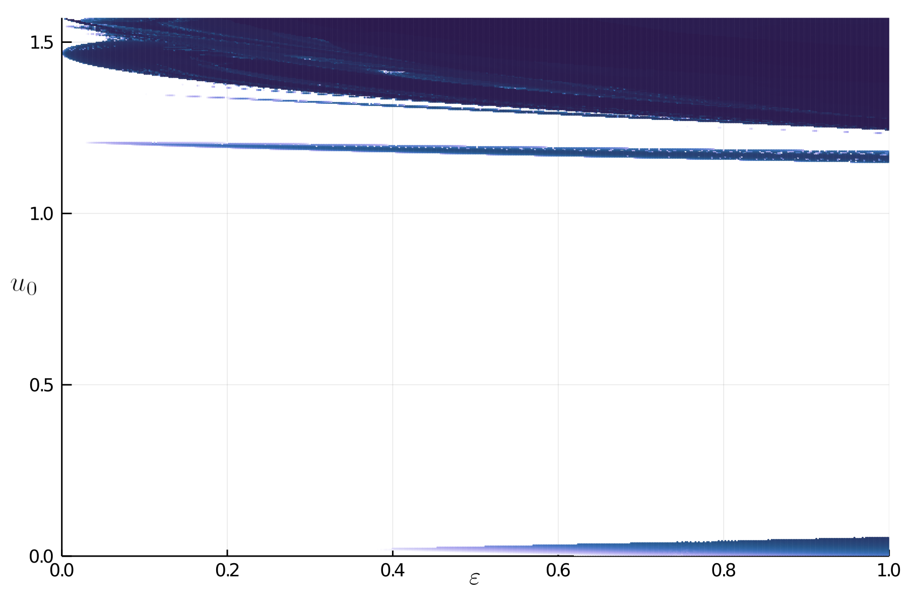
(c) l-foliation, $(\varepsilon,u_{0})\in[0,1]\times[0,\pi/2]$

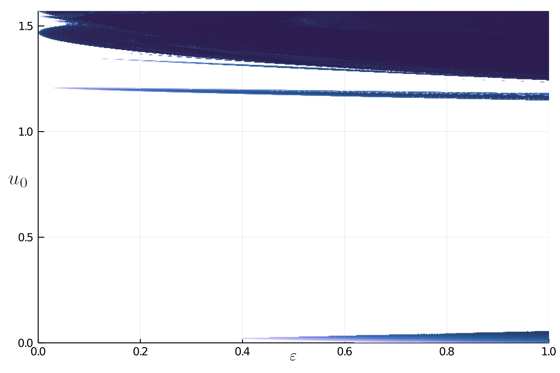
(d) $\psi$-foliation, $(\varepsilon,u_{0})\in[0,1]\times[0,\pi/2]$

Figure 15: Orbits of the Q-flow with $q=4$, that pass the converse KAM condition for time $t_{c}\leq 150$ with initial conditions on the line $(u_{0},u_{0},0)$. Panels (a) and (c) use the l-foliation and (b) and (d) use the $\psi$-foliation. The points are colored according to the time taken to transversality violation, with a darker blue indicating a shorter time.

When $\varepsilon=0$, the orbits of initial conditions with $u_{0}\in(\pi/2,\pi]$ lie in a second cell of $\psi$ contours that is centered at $(\pi,\pi)$. The implication is that orbits may satisfy the converse KAM condition with respect to the l-foliation, as seen in Fig. 15(a), even though they may still lie on tori—now enclosing the elliptic orbit near $(\pi,\pi)$. Indeed when $\varepsilon\ll 1$, most of the orbits in this region do lie on such tori. By contrast, the $\psi$-foliation shown in Fig. 15(b) correctly indicates that there are still tori in this region, since the foliation in this case is essentially radial with respect to the origin at $(\pi,\pi)$.

A further enlargement of Fig. 15(d) is shown in Fig. 16(a). Note that there are many small tongues of destroyed tori just above $u_{0}=\tfrac{\pi}{2}$. These results can be compared to the maximal Lyapunov exponent shown in the right panel. Here initial conditions with $\lambda<0.15$ are—somewhat arbitrarily—deemed to be regular and colored white. A large tongue that emanates from $(u_{0},\varepsilon)=(1.47,0)$ is a regular island chain. As for the two-wave case, it is difficult, using the finite-time Lyapunov exponent for $t=150$, to obtain a sharp distinction between regular and chaotic orbits .

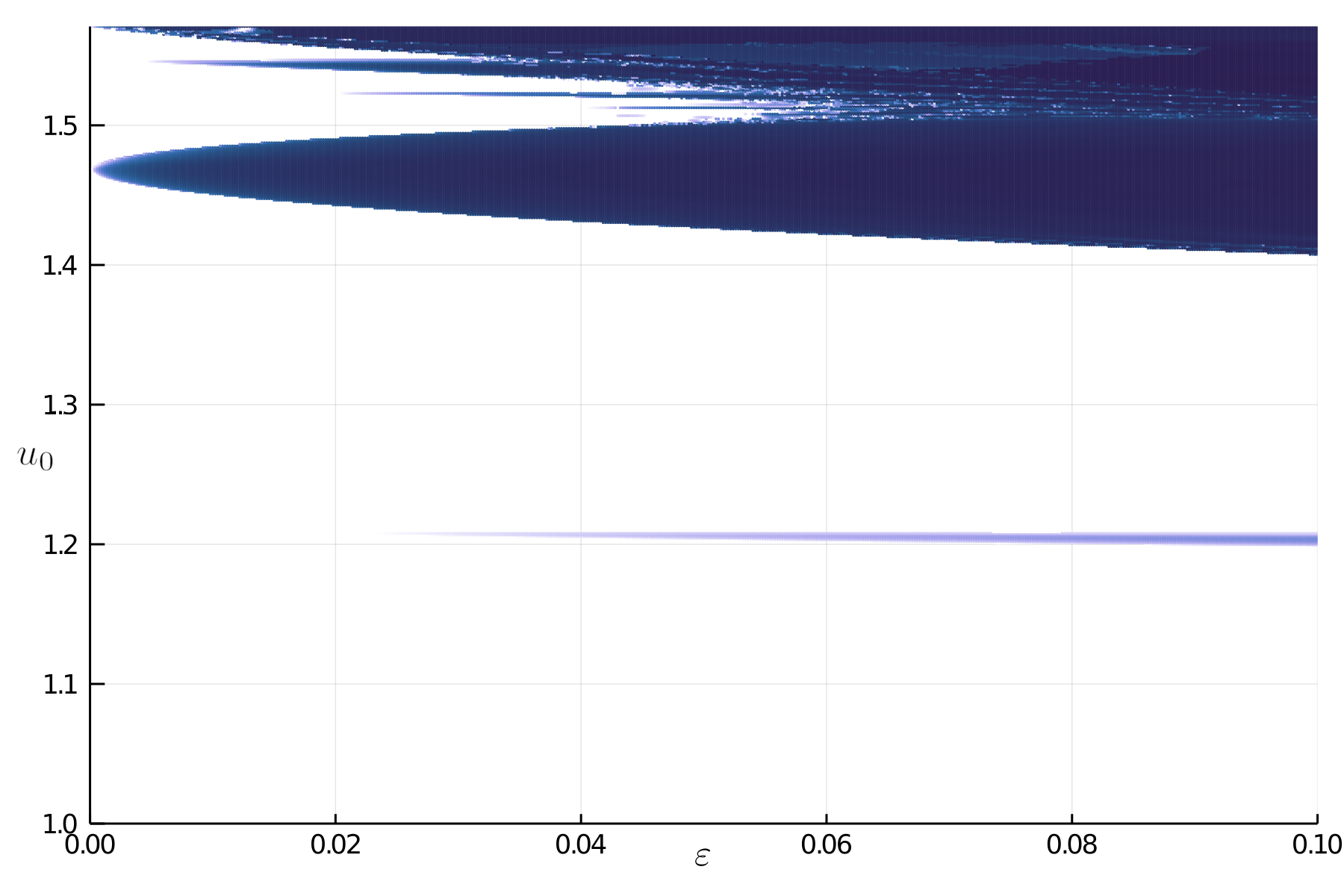
(a) $\psi$-foliation

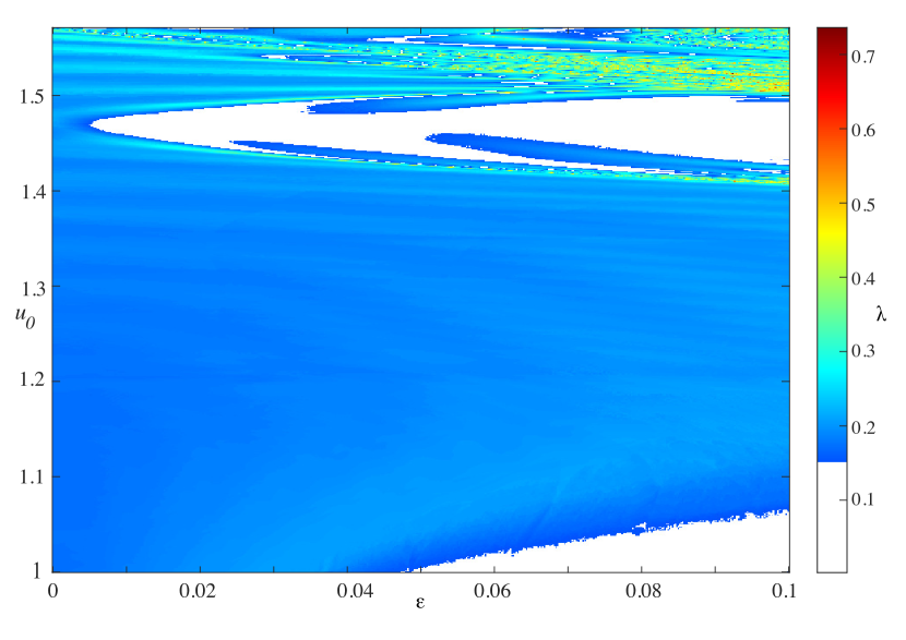
(b) Maximal Lyapunov exponent

Figure 16: Q-flow with $q=4$ for $(\varepsilon,u_{0})\in[0,0.1]\times[1,\pi/2]$. Panel (a) is an enlargement of Fig. 15(d). Panel (b) is the maximal Lyapunov exponent for the orbits of (a) using the initial tangent vector $v_{0}=(0,1,0)$.

Orbits that pass the converse KAM condition for the $q=5$ case, which, as we saw in Fig. 4(a), has quasi-crystal symmetry, are displayed in Fig. 17(a) using the $\psi$-foliation. Here the initial conditions lie on the line $(0,y_{0},0)$. The computations show that there are many tongues that have no tori relative to this foliation. This can be compared to the computations of the Lyapunov exponent in panel (b). Note that, again, the converse KAM condition is much more sensitive to the destruction of tori as it would require a longer computation to get convergence of the exponent.

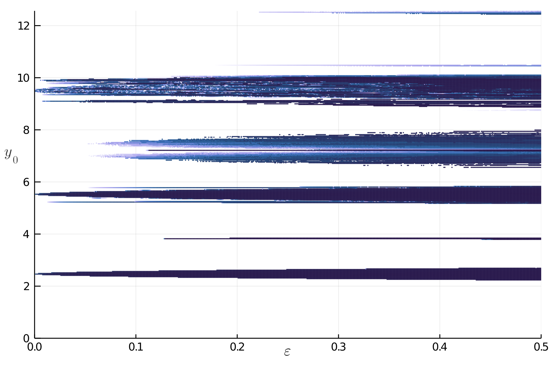
(a) $\psi$-foliation

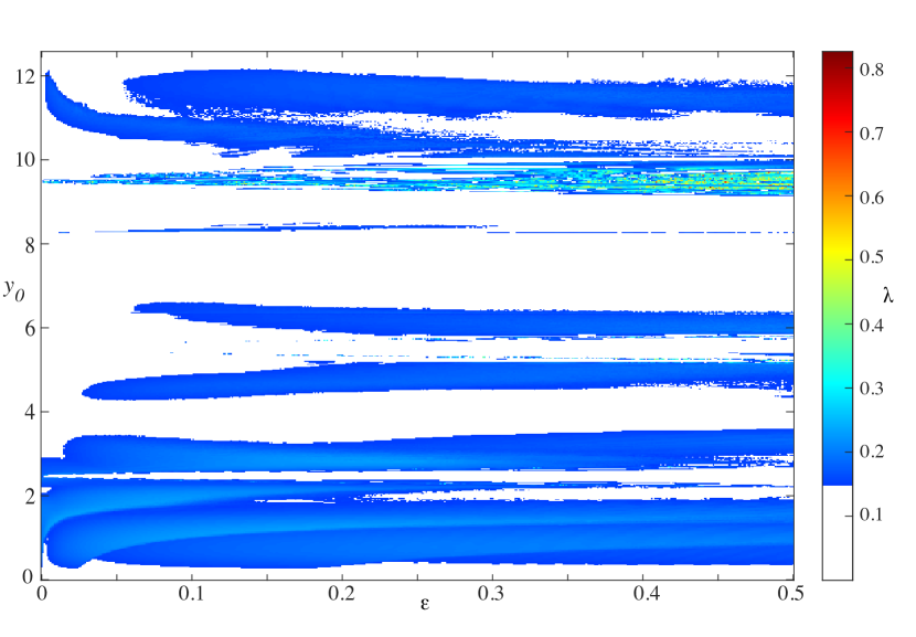
(b) Maximal Lyapunov exponent

Figure 17: Q-flow with $q=5$ for initial conditions on the line $(0,y_{0},0)$ and $(\varepsilon,y_{0})\in[0,0.5]\times[0,4\pi]$. Panel (a) shows orbits that pass the converse KAM condition for the $\psi$-foliation for $t\leq 150$. Panel (b) depicts the maximal Lyapunov exponent for the orbits of Panel (a).

Figure 18(a) shows an enlargement (near $y_{0}=7$) of two of the tongues of Fig. 17(a). A different set of initial conditions,$(x_{0},0,0)$ for $x_{0}$ near $11$ and $\varepsilon\in[0,0.5]$, are shown in panel (b). This panel gives a closer view of the elliptic orbit that passes near $(10.75,0,0)$.

(a) Enlargement of (a)

(b) Initial conditions on the line $(x_{0},0,0)$.

Figure 18: Q-flow with $q=5$. Panel (a) is an enlargement of Fig. 17(a). Panel (c) shows orbits staring on the line $(x_{0},0,0)$ that pass the converse KAM condition.

VI Discussion

We have shown computations of the converse KAM condition for two models using a variety of foliations. We summarize some our results here.

• For the rotational tori, our results agree with those of MacKay.

  The results for the r-foliation in the two-wave model (Fig. 7) are identical to those of (Mac, 89, Fig. 4). This foliation detects when a given point does not lie on a rotational invariant torus that is a graph over $(q,t)$.

• The selection of an appropriate foliation is crucial.

  As was discussed in §IV, the results obtained are sensitive to the choice of foliation. In §V.2, we presented results for four different foliations of the two-wave flow, and, in §V.3, results for two foliations of the Q-flow.

  For the two-wave case, one interesting aspect of the l-foliation, (25), shown in Fig. 8, is that points not on librational tori could be expected to dependently satisfy the converse KAM condition. However, it is apparent in the figure that those points on rotational tori are not dependent. This agrees with the discussion in §IV: the invariant tori of null-homology with respect to $\mathcal{M}=M\setminus\Sigma$ for the singuarlity set $\Sigma$ will satisfy the converse KAM condition dependently. Note that for the l-foliation, $M=\mathbb{T}\times\mathbb{R}\times\mathbb{T}$ and $\Sigma=\bigl{\{}(0,0,t)\bigm{|}t\in\mathbb{T}\bigr{\}}$; thus the rotational tori are not of null-homology, and these tori are transverse to the l-foliation.

  Hidden in Fig. 8 and Fig. 9, for the l- and p-foliations, are small tongues around $p_{0}=0$ that satisfy the converse KAM condition. These result from the elliptic periodic orbit that begins at $(q,p)=(0,0)$ for $\mu=0$, having a nontrivial oscillation when $\mu>0$. By contrast, the singular set of the s1-foliation more accurately tracks the drift of this orbit, so that $\mathcal{M}=M\setminus\Sigma$ agrees better with the homology of the true orbits of the vector field $v$.

  The s1-foliation (Fig. 10) also has an elliptic orbit near $(q,p)=(0,1)$. Thus, rotational tori around the elliptic orbit of the vector field near $(0,1)$ are not of null-homology with respect to this foliation. This gives a more accurate picture of both the rotational tori and the librational tori in the two forced resonances.

• It is difficult to conclude a point lies on no invariant surface.

  In a typical Hamiltonian or volume-preserving flow resonances are dense. Many of these will form island chains, and if one were to find points that do not lie on any invariant surface, one would have to know the locations of all of these resonant island chains.

  For example, the s1-foliation is constructed to ensure that points on rotational, and librational tori around $(0,0)$ and $(0,1)$, are not necessarily dependent. The s2-foliation was designed to also ensure that the 1:2 resonant tori near $(q,p)=(0,\tfrac{1}{2})$ are not dependent. However, it fails to appropriately test for librational tori in the primary elliptic regions; indeed, there are points passing the converse KAM criterion near $p=0$ and $p=1$ in Fig. 12 even though a phase portrait shows there are tori.

  It might be possible to use renormalization procedures to better design a foliation adapted to some resonances, but since there are typically an infinite number of homologies of tori, it seems impossible to detect them all. The methods discussed here could be used to design a foliation appropriate to a particular homology in a localized region of phase space.

• The results depend on choice of initial conditions.

  Figure 14 shows how the results depend on the choice of section for the two-wave model since we only have chosen initial conditions along a line $(0,p_{0},t_{0})$. Though the overall structure is similar to the $t=0$ section in Fig. 10, there are some notable differences.

  The $t=0.25$ section reveals more details about trapped islands in the librational regions about $p_{0}=0$ and $1$ because the initial conditions are closer to the hyperbolic points of these resonances.

  In the $t=0.5$ section there is almost a complete lack of orbits trapped in the librational regions because the line of initial conditions goes through the hyperbolic orbits of these main island chains. If one wants to understand all possible islands, one should take care to choose appropriate initial conditions.

  The importance of the choice of initial conditions is also evident in the Q-flow for $q=5$ by noting the various islands not sampled when taking $x_{0}=0$ in (Fig. 17(a)) compared to $y_{0}=0$ (Fig. 18(b)).

• Finite-time Lyapunov exponents can be less effective.

  Finite-time Lyapunov exponents, shown in Figs. 13, 16(b) and 17(b), are often used to detect chaotic regions. We have seen that the converse KAM criterion accurately detects such regions as well (though it also detects orbits on non-transverse tori). In our computations, we used the same time $t=150$ in both computations, and the distribution of Lyapunov exponents does not give a clear distinction between regular and chaotic orbits. Celletti et al CM (07) note that “in contrast to the Lyapunov exponents, the nonexistence criterion allows us to distinguish between chaotic motions [and] librational tori, and rotational tori, [thus] extending the idea of the fast Lyapunov indicators GLF (02).” This statement is clearly evident as the converse KAM method detects the nonexistent of tori of certain homology.

• The inverse of the converse KAM time gives a measure of librational frequency.

  As White notes Whi (15), the rate of rotation of the phase vector, $\xi_{t}$, for orbits in islands gives a measure of the librational frequency inside the island. This should correlate with a times scale for flattening of a density profile of a passive scalar inside these island chains. As such this could be a useful measure for plasma confinement devices.

In conclusion, the numerical application of Thm. II.3 or Thm. II.4 is extremely useful if one is looking in particular at the existence of invariant surfaces of a given homological type.

Future Directions

Whilst converse KAM theory dates back several decades, we hope that with an appropriate choice of foliation, it can be directly applied to the optimization of fusion confinement devices such as stellarators. For a stellarator to be effective at trapping charged particles, there should be many invariant tori that can act as effective barriers for particle transport. Indeed, integrability or near-integrability is an often used criterion for optimal design of these devices. In this sense, we hope that converse KAM theory can be used to create a rapidly computable measure that would help to design configurations that maximize integrability.

Another potential application is to the construction of divertors; configurations that enhance particle transport at controlled points on the outer surface of the plasma. These allow better control of the plasma boundary and help to control impurities Boo (15). One type of divertor uses a magnetic field with a hyperbolic orbit on the plasma edge BP (18). The positioning of this hyperbolic orbit must be precise. Hence, a foliation could be constructed to test potential magnetic fields for their ability to adhere to the desired divertor configuration.

While converse KAM theory has been applied to detect nonexistence of invariant Lagrangian tori in MMS (89), it does not seem to have been applied more generally to higher-dimensional systems. The ideas we have discussed can search for the nonexistence of invariant surfaces with a fixed Lipschitz constant. The core issue with checking Thm. II.2 for $n>3$ is the codimensionality of the line $\operatorname{Span}(\eta_{t})$, which is one for $n=3$ in $\mathcal{P}$, but in general is $n-2$. Thus, $\xi_{t}$ will almost never cross the line $\eta_{t}$. Given a constraint on the Lipschitz constant of possible invariant surfaces, one then asks if $\xi_{t}$ crosses a cone about $\eta_{t}$. This is again a codimension-one problem.

A converse KAM condition is said to be exhaustive if all orbits that do not lie on surfaces transverse to the chosen foliation $\mathcal{F}$ eventually satisfy the converse KAM condition. This notion is addressed in Mac (18) where it is noted that orbits on some invariant sets (for example cantori) may not satisfy the converse KAM condition even though these are not invariant surfaces. The remedy is to amend the procedure with the so-called “killends” condition MP (85). As argued in Mac (18), this condition allows any orbit in a volume-preserving system not lying on an invariant surface transverse to $\mathcal{F}$ to be detected. However, in general, exhaustiveness is only conjectured. In the future we hope to develop the killends condition to help address this question.

Appendix A Global Removal of Resonances

The approximate invariant (26) is the result of a technique used in §2.4d of LL (92), where it is called “global removal of resonances”. We assume that $M=(\mathbb{T}\times\mathbb{R})^{2}$ with coordinates $(\theta_{1},I_{1},\theta_{2},I_{2})$, where the angles have period one. The technique works for any two degree-of-freedom Hamiltonian that can be written as a perturbation of the integrable Hamiltonian $H_{0}:M\to\mathbb{R}$,

$$H_{0}(I_{1},\theta_{1},I_{2},\theta_{2})=S_{1}(I_{1})+I_{2}.$$ (29)

Note that this requires that the integrable system have global action-angle variables, $I_{i}$ and be separable. We also assume, for simplicity, that the second degree of freedom is harmonic, and without loss of generality set the harmonic frequency to one. Note that such a system also arises from a periodically time-dependent, $1\tfrac{1}{2}$ degree-of-freedom system, such as the two-wave model of §III.1, in extended in extended phase space.

Assume we have a Hamiltonian of the form

$$H(\theta_{1},I_{1},\theta_{2},I_{2})=H_{0}(I_{1},I_{2})+\varepsilon H_{1}(I_{1},\theta_{1},I_{2},\theta_{2})+\dots.$$ (30)

The key observation is that when $\varepsilon\ll 1$, $I_{1}$ will vary slowly; that is, $I_{1}$ is an adiabatic invariant. The question then becomes; can we build a ‘better’ (read ‘higher order’), adiabatic invariant $J$ from $I$?

A function $J:M\to\mathbb{R}$ is invariant whenever

$$\{H,J\}=0,$$ (31)

where $\{\cdot,\cdot\}$ is the canonical Poisson bracket,

$$\{F,G\}=\sum_{i=1}^{n}\frac{\partial F}{\partial I_{i}}\frac{\partial G}{\partial\theta_{i}}-\frac{\partial F}{\partial\theta_{i}}\frac{\partial G}{\partial I_{i}},$$

and we use the convention that the Hamiltonian vector field $X_{H}=\{H,\cdot\}$.

Expanding $J$ in $\varepsilon$,

$$J=J_{0}+\varepsilon J_{1}+\dots,$$

the most obvious direction to proceed is to expand $\{H,J\}$ in $\varepsilon$ and solve the equation at order-by-order in $\varepsilon$. This approach is sufficient for low order calculations, however, if one wants to compute $J$ to higher order, a Lie transform approach is more convenient.

Let us first use the direct method to compute the lowest order invariant. Expanding (31) to first order in $\varepsilon$ gives the two equations,

$$\{H_{0},J_{0}\} =0$$ (32)

$$\{H_{0},J_{1}\} =-\{H_{1},J_{0}\}=\{J_{0},H_{1}\}.$$ (33)

The first condition is satisfied for any $J_{0}=J_{0}(I_{1},I_{2})$. For the examples considered here, it is sufficient to consider $J_{0}$ a function of $I_{1}$ only. Expanding the second equation yields,

$$\omega_{1}(I_{1})\partial_{\theta_{1}}J_{1}+\partial_{\theta_{2}}J_{1}=J_{0}^{\prime}(I_{1})\partial_{\theta_{1}}H_{1}.$$ (34)

where $\omega_{1}=S_{1}^{\prime}$, is the action-dependent frequency of (29). Now, let,

$$H_{1}=\sum_{n,m}h_{n,m}(I_{1},I_{2})\mathrm{e}^{2\pi i(n\theta_{1}+m\theta_{2})},\qquad J_{1}=\sum_{n,m}k_{n,m}(I_{1},I_{2})\mathrm{e}^{2\pi i(n\theta_{1}+m\theta_{2})}.$$ (35)

Substituting these Fourier series into (34) yields,

$$(\omega_{1}n+m)k_{n,m}=J_{0}^{\prime}nh_{n,m}.$$

The solution for $k_{n,m}$ is singular whenever $\omega_{1}n+m=0$, the so called ‘resonances’. However, McNamara had the central idea that, provided one knows which resonances appear in $H_{1}$ a priori, then, through judicious choice of the free function $J_{0}^{\prime}$, it is possible to ensure the right hand side vanishes at resonance, thus obtaining a nonsingular value for $J_{1}$.

Let us apply this theory to the two-wave model. Here we extend the phase space by adding the (negative) energy variable $e$, so that $H\to H+e$ and the canonical form becomes $\omega=dp\wedge dq+de\wedge dt$. Setting $(\theta_{1},I_{1},\theta_{2},I_{2})=(q,p,t,e)$, $\varepsilon=\mu$ and

$$H_{0} =\tfrac{1}{2}p^{2}+e,$$

$$H_{1} =-\cos(2\pi q)-\nu\cos(2\pi k(q-t)).$$

so that $e$ is the negative of the time-dependent energy of the original system (16). Taking,

$$J_{1}=A(p)\cos(2\pi q)+B(p)\cos(2\pi k(q-t)),$$

to match the harmonics of $H_{1}$, then (34) is solved provided,

$$A=-\frac{J_{0}^{\prime}(p)}{p},\qquad B=-\nu\frac{J_{0}^{\prime}(p)}{p-1}.$$ (36)

It is then evident that choosing, for instance, $J_{0}^{\prime}(p)=p(p-1)$ will yield a nonsingular $J_{1}$. In summary, we obtain—to first order—that $J$ is given by (26).

Of course, it is important to ask whether one can use a similar method to obtain higher orders in $\varepsilon$. This is possible to do directly as above; however, making use of some normal form theory and Lie transforms allows for some ease in describing how to do this. This higher order version was first realized in McN (78).

The primary aim of this higher order invariant is to transform the Hamiltonian (30) to the Hamiltonian averaged over the $H_{0}$ trajectories,

$$\bar{H}(\phi_{1},\bar{I}_{1},\phi_{2},\bar{I}_{2})=H_{0}(\bar{I}_{1},\bar{I}_{2})+\varepsilon\bar{H}_{1}(\bar{I}_{1},\bar{I}_{2})+\dots,$$

at least to some order. If this is achieved then the resulting coordinates $\bar{I}_{1},\bar{I}_{2}$ will be nearly invariant and writing $\bar{I}_{1}=\bar{I}_{1}(\theta_{1},I_{1},\theta_{1},I_{2})$ gives the desired invariant in the old coordinates.

A convenient method for obtaining the averaged Hamiltonian is through normal form theory and Lie transforms. Given a function $W:M\to\mathbb{R}$ one can generate the associated Hamiltonian vector field $X_{W}$ through

$$X_{W}:=\{W,\cdot\}.$$

The time-$\varepsilon$ flow of such a vector field, $\phi_{W}^{\varepsilon}=e^{\varepsilon X_{W}}$, is a canonical transformation from the old coordinates $z$ to new coordinates, say $Z=\phi_{W}^{\varepsilon}(z)$. This gives a remarkable connection between functions and near-identity canonical transformations. Moreover, pulling back a function $F$ by $\phi_{W}^{\varepsilon}$, the so called Lie transformation, can be computed from the exponentiation of the vector field,

$$\phi_{W}^{\varepsilon*}F=\mathrm{e}^{\varepsilon X_{W}}F.$$

This is a consequence of the fact that the space of Hamiltonian vector fields $X$ is the Lie algebra associated to the Lie group of canonical transformations. The pullback of a function $F$ by $\phi_{W}^{\varepsilon*}$ can be written in the form

$$\phi_{W}^{\varepsilon*}F=\mathrm{e}^{\varepsilon\mathcal{L}_{W}}F.$$

The Lie transformation view gives a quick method for computing transformed a Hamiltonian under a canonical transform generated from some $W$. In particular, to carry out a normalization at order $\varepsilon^{i}$, we write,

$$H=H_{0}+\varepsilon H_{1}+\dots,\qquad W=\varepsilon^{i-1}W_{i},$$

then the Lie transform method yields the transformed Hamiltonian as,

$$\phi_{W}^{*}H =\mathrm{e}^{X_{W}}H$$

$$=\mathrm{e}^{\varepsilon^{i}\{W,\cdot\}}(H_{0}+\varepsilon H_{1}+\dots)$$

$$=H_{0}+\varepsilon H_{1}+\dots+\varepsilon^{i}(\{W_{i},H_{0}\}+H_{i})+\dots.$$

Hence, if $\phi_{W}^{*}H:=\bar{H}$ then the $\bar{H}_{j}=H_{j}$ for $j<i$ and at order $i$ we have,

$$\{H_{0},W_{i}\}=H_{i}-\bar{H}_{i},$$ (37)

the so call homological equation.

This observation gives a method for computing the averaged Hamiltonian $\bar{H}$ by sequentially solving each order $i$. The operator $\mathcal{L}_{H_{0}}:=\{H_{0},\cdot\}$ is known as the cohomological operator. For the two-wave example it is given by,

$$\mathcal{L}_{H_{0}}=p\partial_{q}+\partial_{t}.$$

Equation (37) can be solved by taking Fourier series as in (35). However the solution will be singular at resonance.

To obtain an integral that is not singular, despite the averaged Hamiltonian being singular, we can apply the inverse transformation generated by the $W_{i}$ to an arbitrary function $\tilde{J}_{0}(\bar{I}_{1})$. The inverse transformation is acquired through the composition of each of the $-W_{i}$ generated transformations. In particular, the lowest order terms would be,

$$J(\theta_{1},I_{1},\theta_{2},I_{2}) =e^{-\varepsilon^{2}X_{W_{2}}}e^{-\varepsilon X_{W_{1}}}\tilde{J}_{0}$$

$$=\tilde{J}_{0}(I_{1})-\varepsilon\{W_{1},\tilde{J}_{0}\}+\varepsilon^{2}\left(-\{W_{2},\tilde{J}_{0}\}+\tfrac{1}{2}\{W_{1},\{W_{1},\tilde{J}_{0}\}\}\right)+\dots.$$

Hence, in order $J_{0}$ be nonsingular, $\tilde{J}_{0}$ must be chosen to cancel the singularities in both $W_{2}$ and $W_{1}$.

Using the outlined procedure a second order adiabatic invariant for the two-wave model can be computed as,

$$J =\tfrac{1}{4}(p-1)^{4}p^{4}-\mu\left(p^{2}(2p-1)(p-1)^{3}\cos(2\pi q)+\nu p^{3}(2p-1)(p-1)^{2}\cos(2\pi(q-t))\right)$$ (38)

$$\qquad+\tfrac{1}{4}\mu^{2}\left[\nu^{2}p^{2}(10p^{2}-12p+3)+\nu^{2}p^{2}(3p-1)(4p-3)\cos(4\pi(q-t))\right.$$

$$\qquad\quad+4\nu p(p-1)(6p^{2}-6p+1)\cos(2\pi(2q-t))+\nu p(5p^{2}-5p+1)\cos(2\pi t))$$

$$\qquad\quad\left.+(3p-2)(4p-1)(p-1)^{2}\cos(4\pi q)+(10p^{2}-8p+1)(p-1)^{2}\right]$$

References

- Boo (15) A.H. Boozer. Stellarator design. Journal of Plasma Physics, 81(6):515810606, 2015. https://www.cambridge.org/core/article/stellarator-design/520178F88588D5631663E191EF6C6CE2.
- BP (18) A.H. Boozer and A. Punjabi. Simulation of stellarator divertors. Physics of Plasmas, 25(9):092505, 2018. https://doi.org/10.1063/1.5042666.
- CM (07) A. Celletti and R.S. MacKay. Regions of nonexistence of invariant tori for spin-orbit models. Chaos, 17(4):043119, 12, 2007. https://doi.org/10.1063/1.2811880.
- DFG+ (86) T. Dombre, U. Frisch, J.M. Greene, M. Hénon, A. Mehr, and A.M. Soward. Chaotic streamlines in the abc flows. J. Fluid Mech., 167:353–391, 1986. https://doi.org/10.1017/S0022112086002859.
- ED (81) D. F. Escande and F. Doveil. Renormalization method for computing the threshold of the large-scale stochastic instability in two degrees of freedom Hamiltonian systems. Journal of Statistical Physics, 26(2):257–284, October 1981.
- GLF (02) M. Guzzo, E. Lega, and C. Froeschle. On the numerical detection of the effective stability of chaotic motions in quasi-integrable systems. Physica D, 163(1-2):1–25, 2002. https://doi.org/10.1016/S0167-2789(01)00383-9.
- GO (08) D.A. Gomes and A. Oberman. Viscosity solutions methods for converse kam theory. ESAIM. Mathematical Modelling and Numerical Analysis, 42(6):1047–1064, 2008. http://dx.doi.org/10.1051/m2an:2008035.
- Gre (79) J.M. Greene. A method for determining a stochastic transition. J. Math. Phys., 20:1183–1201, 1979. https://doi.org/10.1063/1.524170.
- Har (99) A. Haro. Converse KAM theory for monotone positive symplectomorphisms. Nonlinearity, 12(5):1299–1322, 1999. https://doi.org/10.1088/0951-7715/12/5/306.
- Jun (91) I. Jungreis. A method for proving that monotone twist maps have no invariant circles. Erg. Th. Dyn. Sys., 11:79–84, 1991. https://doi.org/10.1017/S0143385700006027.
- Kna (90) A. Knauf. Closed orbits and converse KAM theory. Nonlinearity, 3:961–973, 1990. https://doi.org/10.1088/0951-7715/3/3/019.
- LL (92) A. J. Lichtenberg and M. A. Lieberman. Regular and Chaotic Dynamics, volume 38 of Applied Mathematical Sciences. Springer New York, 1992.
- Mac (89) R. S. MacKay. A criterion for non-existence of invariant tori for Hamiltonian systems. Physica D, 36(1):64–82, June 1989. https://doi.org/10.1016/0167-2789(89)90248-0.
- Mac (18) R.S. MacKay. Finding the Complement of the Invariant Manifolds Transverse to a Given Foliation for a 3D Flow. Regular and Chaotic Dynamics, 23(6):797–802, November 2018. https://doi.org/10.1134/S1560354718060126.
- Mat (84) J.N. Mather. Non-existence of invariant circles. Erg. Th. Dyn. Sys., 4:301–309, 1984. https://doi.org/10.1017/S0143385700002455.
- Mat (86) J.N. Mather. A criterion for non-existence of invariant circles. Publ. Math. I.H.E.S., 63:153–204, 1986. http://www.springerlink.com/content/w533532g54501m14/fulltext.pdf.
- McN (78) B. McNamara. Super‐convergent adiabatic invariants with resonant denominators by lie transforms. Journal of Mathematical Physics, 19(10):2154–2164, 1978. Publisher: American Institute of Physics.
- Mei (92) J.D. Meiss. Symplectic maps, variational principles, and transport. Rev. Mod. Phys., 64(3):795–848, 1992. https://doi.org/10.1103/RevModPhys.64.795.
- MMS (89) R S MacKay, J D Meiss, and J Stark. Converse KAM theory for symplectic twist maps. Nonlinearity, 2(4):555–570, November 1989.
- MP (85) R.S. MacKay and I.C. Percival. Converse KAM: Theory and practice. Comm. Math. Phys., 98:469–512, 1985. https://doi.org/10.1007/BF01209326.
- Tsi (11) Ch. Tsitouras. Runge–Kutta pairs of order 5(4) satisfying only the first column simplifying assumption. Computers & Mathematics with Applications, 62(2):770–775, July 2011.
- Whi (11) R B White. Modification of particle distributions by magnetohydrodynamic instabilities II. Plasma Physics and Controlled Fusion, 53(8):085018, August 2011.
- Whi (12) R.B. White. Modification of particle distributions by MHD instabilities I. Communications in Nonlinear Science and Numerical Simulation, 17(5):2200–2214, May 2012.
- Whi (15) R B White. Determination of broken KAM surfaces for particle orbits in toroidal confinement systems. Plasma Physics and Controlled Fusion, 57(11):115008, November 2015.
- Zas (91) G. M. Zaslavsky. Dynamical theory and mixing. In Arne V. Johansson and P. Henrik Alfredsson, editors, Advances in Turbulence 3, pages 243–256. Springer, 1991.