Anomalous dimensions from gauge couplings in SMEFT with right-handed neutrinos

Abstract

Standard Model Neutrino Effective Field Theory (SMNEFT) is an effective theory with Standard Model (SM) gauge-invariant operators constructed only from SM and right-handed neutrino fields. For the full set of dimension-six SMNEFT operators, we present the gauge coupling terms of the one-loop anomalous dimension matrix for renormalization group evolution (RGE) of the Wilson coefficients between a new physics scale and the electroweak scale. We find that the SMNEFT operators can be divided into five subsets which are closed under RGE. Our results apply for both Dirac and Majorana neutrinos. We also discuss the operator mixing pattern numerically and comment on some interesting phenomenological implications.

1 Introduction

The Standard Model (SM) of particle physics is an effective theory valid to some mass scale $\Lambda$. New physics at the scale $\Lambda$ may address important issues like the origin of the electroweak scale, $\mu_{EW}$. In the SM, electroweak symmetry breaking arises from a complex fundamental Higgs scalar. Between $\mu_{EW}$ and $\Lambda$, an effective field theory (EFT) framework can be used to describe new physics in a model independent way. In this approach, the leading terms are given by the SM, and corrections from an underlying theory beyond the SM are described by higher dimension operators,

$${\cal L}=\sum_{i}{\cal{C}}_{i}{\cal O}_{i}\,.\$$ (1)

The operators ${\cal O}_{i}$ are $SU(3)_{C}\times SU(2)_{L}\times U(1)_{Y}$ invariant and are constructed only from SM fields. The Wilson coefficients (WCs) ${\cal{C}}_{i}$, that determine the size of the contribution of operators ${\cal O}_{i}$, can be calculated by matching the effective theory with the underlying theory.

Analyses of higher dimension operators Buchmuller:1985jz have begun anew in the study of the SM as an effective field theory. Due to the phenomenological success of the SM gauge theory and the Higgs mechanism, the most studied EFT is the Standard Model Effective Field Theory (SMEFT) Grzadkowski:2010es ; Henning:2014wua ; Brivio:2017vri , which respects the SM gauge symmetry with only SM field content. The one-loop renormalization group evolution (RGE) of all dimension-six operators in SMEFT have been calculated in Refs. Jenkins:2013zja ; Jenkins:2013wua ; Alonso:2013hga .

In the SMEFT framework, new physics is considered to be heavy with $\Lambda\gg\mu_{EW}$. However, many experiments point to new physics with a mass scale well below the electroweak scale, and many experiments to search for new light states are planned. Since these states do not appear in SMEFT, its Lagrangian must be supplemented by interactions between these new states and the SM fields. Possible new states are right-handed neutrinos that are sterile under SM gauge interactions. The masses of the sterile neutrinos can vary over a large range and can be heavy or light compared to the electroweak scale. Light sterile neutrinos have been invoked to explain many phenomena; see Ref. Abazajian:2012ys for a review.

In this paper, we consider the sterile neutrinos to be light so that they appear as explicit degree of freedoms in the EFT framework. We use the Standard Model Neutrino Effective Field Theory (SMNEFT) which augments SMEFT with right-handed (RH) neutrinos $n$ delAguila:2008ir ; Aparici:2009fh ; Bhattacharya:2015vja ; Liao:2016qyd ; Bischer:2019ttk . The RGE of some SMNEFT operators have been calculated. The mixing between the bosonic operators has been calculated in Refs. Bell:2005kz ; Chala:2020pbn , and the one-loop RGE of a subset of four-fermion operators are given in Ref. Han:2020pff . In this work, we present the gauge terms of the one-loop RGE of all dimension-six operators in SMNEFT.

The paper is organized as follows. In section 2, we define SMNEFT and establish our notation. Our diagrammatic approach to calculate the one-loop anomalous dimension matrix (ADM) is described in section 3. In section 4, we present the ADM. In section 5, we study operator mixing using the leading-log approximation. We discuss some phenomenological implications in section 6, and summarize in section 7. Details of our calculations are provided in an appendix.

2 SMNEFT

In this section, we present SMNEFT. Neutrinos may be Dirac or Majorana. In the case of Dirac neutrinos, $\nu_{R}\equiv n$, with $n$ and the left-handed neutrino $\nu_{L}$ in the same spinor $\nu_{D}=(\nu_{L},n)^{T}$, and of the same mass. In the Majorana case, $n$ and $\nu_{L}$ are components of two different spinors, $\nu_{M}=(\nu_{L},\nu_{L}^{c})^{T}$, $n_{M}=(n^{c},n)^{T}$, and can have different masses. Our results are valid for both cases because we focus on the gauge sector. Without specifying any possible Majorana and Dirac mass terms, the dimension-six $B$ and $L$ conserving SMNEFT Lagrangian is

$$\mathscr{L}^{(6)}_{\text{SMNEFT}}\supset\mathscr{L}_{\rm{SM}}+i\bar{n}\not{\partial}n+\sum_{i}\mathcal{C}_{i}\mathcal{O}_{i}\,,$$ (2)

where $\mathcal{C}_{i}$ are the WCs with the scale of new physics absorbed in them, and the SM Lagrangian is given by

$$\mathscr{L}_{\rm SM}= = -\frac{1}{4}G_{\mu\nu}^{A}G^{A\mu\nu}-\frac{1}{4}W_{\mu\nu}^{I}W^{I\mu\nu}-\frac{1}{4}B_{\mu\nu}B^{\mu\nu}$$ (3)

$$+ (D_{\mu}\phi)^{\dagger}(D^{\mu}\phi)+m^{2}\phi^{\dagger}\phi-\frac{\lambda}{2}(\phi^{\dagger}\phi)^{2}$$

$$+ i(\bar{\ell}\not{D}\ell+\bar{e}\not{D}e+\bar{q}\not{D}q+\bar{u}\not{D}u+\bar{d}\not{D}d)$$

$$- (\bar{\ell}Y_{e}e\phi+\bar{q}Y_{u}u\tilde{\phi}+\bar{q}Y_{d}d\phi+\rm{h.c.})\,.$$

Here, $\tilde{\phi}^{j}=\epsilon_{jk}(\phi^{k})^{*}$, and the Higgs vacuum expectation value is $\langle\phi\rangle=v/\sqrt{2}$ with $v=246$ GeV. The covariant derivative and field strength tensors are defined by

$$D_{\mu}=\partial_{\mu}+ig_{1}yB_{\mu}+ig_{2}\frac{\tau^{I}}{2}W^{I}_{\mu}+ig_{3}\frac{T^{a}}{2}G^{a}_{\mu}\,,$$ (4)

$$B_{\mu\nu} = \partial_{\mu}B_{\nu}-\partial_{\nu}B_{\mu}\,,$$ (5)

$$W^{I}_{\mu\nu} = \partial_{\mu}W_{\nu}^{I}-\partial_{\nu}W_{\mu}^{I}-g_{2}\epsilon^{IJK}W_{\mu}^{J}W_{\nu}^{K}\,,$$ (6)

$$G^{a}_{\mu\nu} = \partial_{\mu}G_{\nu}^{a}-\partial_{\nu}G_{\mu}^{a}-g_{3}f^{abc}G_{\mu}^{b}G_{\nu}^{c}\,,$$ (7)

where $g_{1}$, $g_{2}$, and $g_{3}$ are the gauge couplings of $U(1)_{Y}$, $SU(2)_{L}$, and $SU(3)_{C}$, respectively, and $y$ is the hypercharge. $\epsilon^{IJK}$ and $f^{abc}$ are the $SU(2)_{L}$ and $SU(3)_{C}$ structure constants, respectively.

The 16 baryon and lepton number conserving ($\Delta B=\Delta L$ =0 ) operators involving the field $n$ in SMNEFT are shown in Table 1 Liao:2016qyd in the WCxf convention Aebischer:2017ugx .

$(\bar{R}R)(\bar{R}R)$		$(\bar{L}L)(\bar{R}R)$		$(\bar{L}R)(\bar{R}L)$ and $(\bar{L}R)(\bar{L}R)$
$\mathcal{O}_{nd}$	$(\bar{n}_{p}\gamma_{\mu}n_{r})(\bar{d}_{s}\gamma^{\mu}d_{t})$	$\mathcal{O}_{qn}$	$(\bar{q}_{p}\gamma_{\mu}q_{r})(\bar{n}_{s}\gamma^{\mu}n_{t})$	$\mathcal{O}_{\ell n\ell e}$	$(\bar{\ell}^{j}_{p}n_{r})\epsilon_{jk}(\bar{\ell}^{k}_{s}e_{t})$
$\mathcal{O}_{nu}$	$(\bar{n}_{p}\gamma_{\mu}n_{r})(\bar{u}_{s}\gamma^{\mu}u_{t})$	$\mathcal{O}_{\ell n}$	$(\bar{\ell}_{p}\gamma_{\mu}\ell_{r})(\bar{n}_{s}\gamma^{\mu}n_{t})$	$\mathcal{O}_{\ell nqd}^{(1)}$	$(\bar{\ell}^{j}_{p}n_{r})\epsilon_{jk}(\bar{q}^{k}_{s}d_{t})$
$\mathcal{O}_{ne}$	$(\bar{n}_{p}\gamma_{\mu}n_{r})(\bar{e}_{s}\gamma^{\mu}e_{t})$			$\mathcal{O}_{\ell nqd}^{(3)}$	$(\bar{\ell}^{j}_{p}\sigma_{\mu\nu}n_{r})\epsilon_{jk}(\bar{q}^{k}_{s}\sigma^{\mu\nu}d_{t})$
$\mathcal{O}_{nn}$	$(\bar{n}_{p}\gamma_{\mu}n_{r})(\bar{n}_{s}\gamma^{\mu}n_{t})$			$\mathcal{O}_{\ell nuq}$	$(\bar{\ell}^{j}_{p}n_{r})(\bar{u}_{s}q^{j}_{t})$
$\mathcal{O}_{nedu}$	$(\bar{n}_{p}\gamma_{\mu}e_{r})(\bar{d}_{s}\gamma^{\mu}u_{t})$
$\psi^{2}\phi^{3}$		$\psi^{2}\phi^{2}D$		$\psi^{2}X\phi$
$\mathcal{O}_{n\phi}$	$(\phi^{\dagger}\phi)(\bar{l}_{p}n_{r}\tilde{\phi})$	$\mathcal{O}_{\phi n}$	$i(\phi^{\dagger}\overset{\leftrightarrow}{D}_{\mu}\phi)(\bar{n}_{p}\gamma^{\mu}n_{r})$	$\mathcal{O}_{nW}$	$(\bar{\ell}_{p}\sigma^{\mu\nu}n_{r})\tau^{I}\tilde{\phi}W_{\mu\nu}^{I}$
		$\mathcal{O}_{\phi ne}$	$i(\tilde{\phi}^{\dagger}D_{\mu}\phi)(\bar{n}_{p}\gamma^{\mu}e_{r})$	$\mathcal{O}_{nB}$	$(\bar{\ell}_{p}\sigma^{\mu\nu}n_{r})\tilde{\phi}B_{\mu\nu}$

Table 1: The 16 SMNEFT operators involving RH neutrinos $n$ in the Warsaw basis convention which conserve baryon and lepton number $(\Delta B=\Delta L=0)$. The flavor indices $`prst`$ on the operators are suppressed for simplicity. The fundamental $SU(2)_{L}$ indices are denoted by $i,j$, and $I$ is the adjoint index.

3 Formalism

The anomalous dimensions of an operator are given by the infinite pieces, i.e., the coefficients of the $1/\varepsilon$ terms of the diagrams. In this section, we define our procedure to calculate the ADM, and relegate the details of our calculations to Appendix A. To compute the ADM we use the master formulae presented in Ref. Buras:1998raa . We compute one-loop contributions to the ADM due to SM gauge couplings. The four-fermion operators ($\psi^{4}$) in Table 1 can be divided into four categories: $(\bar{R}R)(\bar{R}R)$, $(\bar{L}L)(\bar{R}R)$, $(\bar{L}R)(\bar{R}L)$, and $(\bar{L}R)(\bar{L}R)$ on the basis of the chiralities of the fields. The remaining operators are of the form $\psi^{2}\phi^{3}$, $\psi^{2}\phi^{2}D$ and $\psi^{2}X\phi$. We focus on the $\psi^{4}$-$\psi^{4}$ and $\psi^{4}$ - $\psi^{2}\phi^{2}D$ operator mixing since the mixing between $\psi^{2}\phi^{3}$, $\psi^{2}\phi^{2}D$ and $\psi^{2}X\phi$ has been computed in the Ref. Chala:2020pbn using the background field method. We have checked that the resulting $5\times 5$ matrix is consistent with the result for the corresponding SMEFT operators Alonso:2013hga which have a similar ADM structure.

For the $\psi^{4}$ operators the bare and renormalized operators are related by

$$\langle{\vec{\mathcal{O}}}\rangle^{(0)}={{Z_{\psi_{1}}^{-\frac{1}{2}}}{Z_{\psi_{2}}^{-\frac{1}{2}}}{Z_{\psi_{3}}^{-\frac{1}{2}}}{Z_{\psi_{4}}^{-\frac{1}{2}}}}~{}{\hat{Z}}\langle\vec{\mathcal{O}}\rangle=Z\langle\vec{\mathcal{O}}\rangle\,,$$ (8)

where the superscript $(0)$ labels the bare matrix elements. Here, $\hat{Z}$ and $Z_{\psi}$ are the renormalization constants for the operator $\vec{\mathcal{O}}$ and the fields $\psi$, respectively. In the $\overline{\rm MS}$ scheme at one-loop level, the renormalization constants take the form,

$$(Z_{m})_{\psi} = 1+\frac{\alpha_{m}}{4\pi}\frac{1}{\varepsilon}a^{m}_{\psi}\,,$$ (9)

$$(Z_{m})_{ij} = \delta_{ij}+\frac{\alpha_{m}}{4\pi}\frac{1}{\varepsilon}b^{m}_{ij}\,,$$ (10)

$$(\hat{Z}_{m})_{ij} = \delta_{ij}+\frac{\alpha_{m}}{4\pi}\frac{1}{\varepsilon}c^{m}_{ij}\,,$$ (11)

with $\psi=\{q,u,d,\ell,e\}$ and $Z_{n}=1$. The coupling constants are defined by $\alpha_{m}={g_{m}^{2}}/{4\pi}$ with $m=1$, 2, 3 for $U(1)_{Y}$, $SU(2)_{L}$ and $SU(3)_{C}$, respectively. The coefficients of the UV divergent parts of the diagrams ($\alpha_{m}/(4\pi\varepsilon)$), $a^{m}_{\psi}$, $b^{m}_{ij}$ and $c^{m}_{ij}$, are independent of the gauge couplings. Note that $c^{m}_{ij}$ can be related to $a^{m}_{\psi}$ and $b^{m}_{ij}$ via Eq. (8). The anomalous dimension matrices are defined by the RG equations,

$$\dot{\mathcal{C}}_{i}(\mu)=16\pi^{2}\mu\frac{d}{d\mu}{\cal C}_{i}(\mu)={(\gamma_{\mathcal{C}})}_{ij}{\cal C}_{j}(\mu),$$ (12)

where $\gamma_{\mathcal{C}}=\gamma^{T}$ with $\gamma$ given by the matrix ${\hat{Z}}$ as

$$\frac{\gamma}{16\pi^{2}}={\hat{Z}}^{-1}\frac{d{\hat{Z}}}{d~{}{\rm\ln}~{}\mu}\,,$$ (13)

and which can be directly expressed in terms of $a^{m}_{\psi}$ and $b^{m}_{ij}$:

$$\gamma_{ij}=-2g_{m}^{2}\left(\sum_{\psi=\psi_{1},..\psi_{4}}\frac{1}{2}a^{m}_{\psi}\delta_{ij}+b^{m}_{ij}\right)\,.$$ (14)

Here, the sum is over external fields $\psi_{1}$ to $\psi_{4}$ in a given operator, and summation over $m$ is implicit. Therefore, in order to compute the ADM for a set of operators, we need to calculate the coefficients $a^{m}_{\psi}$ and $b^{m}_{ij}$ from the field strength renormalization and operator renormalization, respectively.

For the mixing between $\psi^{4}$-$\psi^{4}$ and $\psi^{4}$-$\psi^{2}\phi^{2}D$, the current-current (Fig. 1) and penguin (Fig. 2) topologies mediated by the gauge bosons $X_{\mu}=B_{\mu},W_{\mu},G_{\mu}$, or the scalar, have to be calculated. These diagrams can be computed by easily generalizing the master formulae of Ref. Buras:1998raa to SMNEFT; see Eqs. (53)-(59).

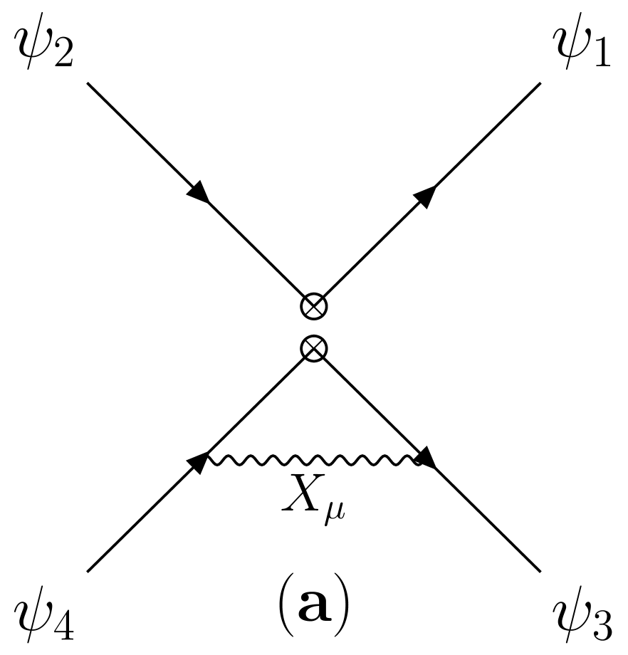
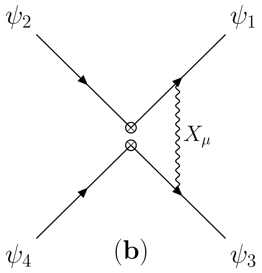
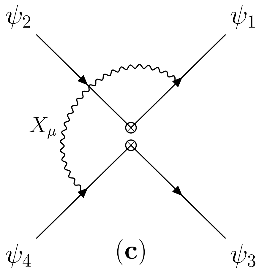
Figure 1: Current-current topologies with four-fermion insertions. Here $X_{\mu}$ represents the gauge bosons $B_{\mu}$, $W_{\mu}$ and $G_{\mu}$. The fermion fields $q,u,d,\ell,e$ and $n$ are represented by $\psi_{I}$.

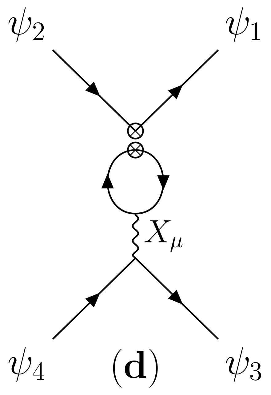
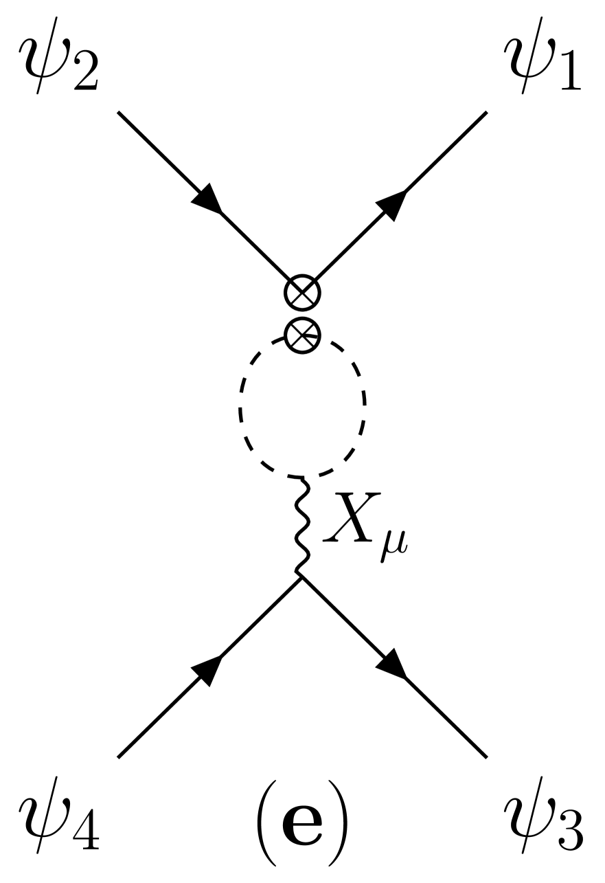
Figure 2: Penguin topologies with four-fermion (d) and boson (e) insertions.

In Appendix A, we present explicit calculations of the ADMs for $\mathcal{O}_{nd}-\mathcal{O}_{nd}$, $\mathcal{O}_{\phi n}-\mathcal{O}_{nd}$, $\mathcal{O}_{nedu}-\mathcal{O}_{nedu}$ and $\mathcal{O}_{\ell n\ell e}-\mathcal{O}_{\ell n\ell e}$ operator mixing. The same method is applicable to the other operators. It is worth noting that for most of the cases the structure of the ADMs of the SMNEFT operators are similar to those of SMEFT operators Alonso:2013hga . Therefore, our SMNEFT results also serve as an important cross-check for the corresponding gauge terms appearing in the SMEFT ADMs.

4 Anomalous dimensions

We now present terms for the one-loop ADM that depend on the gauge couplings $\alpha_{1}$, $\alpha_{2}$ and $\alpha_{3}$ for all 16 SMNEFT operators. The general formula for the ADM is given by Eq. (14) and details of the calculations of the Feynman diagrams to extract $a^{m}_{\psi}$ and $b^{m}_{ij}$ can be found in Appendix A. The ADM for bosonic SMNEFT operators is given in Ref. Chala:2020pbn . The ADM of most SMNEFT operators can be obtained from the ADM of the SMEFT operators Alonso:2013hga with a similar structure. For example, the ADM for the SMNEFT operators $\mathcal{O}_{\ell nuq}$, $\mathcal{O}^{(1)}_{\ell nqd}$ and $\mathcal{O}^{(3)}_{\ell nqd}$, can be obtained by replacing $e$ with $n$, and switching $u$ and $d$ in the SMEFT operators $\mathcal{O}_{\ell edq}$, $\mathcal{O}^{(1)}_{\ell equ}$ and $\mathcal{O}^{(3)}_{\ell equ}$. We use this procedure as a cross-check when available. No such comparison is possible for $\mathcal{O}_{nedu}$, which has a structure not present in SMEFT.

4.1 $\psi^{4}$

The ADM for four-fermion operators are provided below.

4.1.1 $(\bar{R}R)(\bar{R}R)$

$$\dot{\mathcal{C}}_{\underset{prst}{nd}} = (\frac{4}{3}N_{c}y_{d}^{2}\mathcal{C}_{\underset{prww}{nd}}+\frac{4}{3}N_{c}y_{d}y_{u}\mathcal{C}_{\underset{prww}{nu}}+\frac{4}{3}y_{d}y_{e}\mathcal{C}_{\underset{prww}{ne}}+\frac{8}{3}N_{c}y_{d}y_{q}\mathcal{C}_{\underset{wwpr}{qn}}+\frac{8}{3}y_{d}y_{\ell}\mathcal{C}_{\underset{wwpr}{\ell n}}$$ (15)

$$+\frac{4}{3}y_{d}y_{h}\mathcal{C}_{\underset{pr}{\phi n}}){g_{1}^{2}}\delta_{st}\,,$$

$$\dot{\mathcal{C}}_{\underset{prst}{nu}} = (\frac{4}{3}N_{c}y_{u}y_{d}\mathcal{C}_{\underset{prww}{nd}}+\frac{4}{3}N_{c}y_{u}^{2}\mathcal{C}_{\underset{prww}{nu}}+\frac{4}{3}y_{u}y_{e}\mathcal{C}_{\underset{prww}{ne}}+\frac{8}{3}N_{c}y_{u}y_{q}\mathcal{C}_{\underset{wwpr}{qn}}+\frac{8}{3}y_{u}y_{\ell}\mathcal{C}_{\underset{wwpr}{\ell n}}$$ (16)

$$+\frac{4}{3}y_{u}y_{h}\mathcal{C}_{\underset{pr}{\phi n}}){g_{1}^{2}}\delta_{st}\,,$$

$$\dot{\mathcal{C}}_{\underset{prst}{ne}} = (\frac{4}{3}N_{c}y_{e}y_{d}\mathcal{C}_{\underset{prww}{nd}}+\frac{4}{3}N_{c}y_{e}y_{u}\mathcal{C}_{\underset{prww}{nu}}+\frac{4}{3}y_{e}^{2}\mathcal{C}_{\underset{prww}{ne}}+\frac{8}{3}N_{c}y_{e}y_{q}\mathcal{C}_{\underset{wwpr}{qn}}+\frac{8}{3}y_{e}y_{\ell}\mathcal{C}_{\underset{wwpr}{\ell n}}$$ (17)

$$+\frac{4}{3}y_{e}y_{h}\mathcal{C}_{\underset{pr}{\phi n}}){g_{1}^{2}}\delta_{st}\,,$$

$$\dot{\mathcal{C}}_{\underset{prst}{nedu}} = ((y_{d}-y_{u})^{2}+y_{e}(y_{e}+8y_{u}-2y_{d})){g_{1}^{2}}\mathcal{C}_{\underset{prst}{nedu}}\,,$$ (18)

$$\dot{\mathcal{C}}_{\underset{prst}{nn}} = 0\,,$$ (19)

4.1.2 $(\bar{L}L)(\bar{R}R)$

$$\dot{\mathcal{C}}_{\underset{prst}{qn}} = (\frac{4}{3}N_{c}y_{q}y_{d}\mathcal{C}_{\underset{stww}{nd}}+\frac{4}{3}N_{c}y_{q}y_{u}\mathcal{C}_{\underset{stww}{nu}}+\frac{4}{3}y_{q}y_{e}\mathcal{C}_{\underset{stww}{ne}}+\frac{8}{3}N_{c}y_{q}^{2}\mathcal{C}_{\underset{wwst}{qn}}+\frac{8}{3}y_{q}y_{\ell}\mathcal{C}_{\underset{wwst}{\ell n}}$$ (20)

$$+\frac{4}{3}y_{q}y_{h}\mathcal{C}_{\underset{st}{\phi n}}){g_{1}^{2}}\delta_{pr}\,,$$

$$\dot{\mathcal{C}}_{\underset{prst}{\ell n}} = (\frac{4}{3}N_{c}y_{\ell}y_{d}\mathcal{C}_{\underset{stww}{nd}}+\frac{4}{3}N_{c}y_{\ell}y_{u}\mathcal{C}_{\underset{stww}{nu}}+\frac{4}{3}y_{\ell}y_{e}\mathcal{C}_{\underset{stww}{ne}}+\frac{8}{3}N_{c}y_{\ell}y_{q}\mathcal{C}_{\underset{wwst}{qn}}+\frac{8}{3}y_{\ell}^{2}\mathcal{C}_{\underset{wwst}{\ell n}}$$ (21)

$$+\frac{4}{3}y_{\ell}y_{h}\mathcal{C}_{\underset{st}{\phi n}}){g_{1}^{2}}\delta_{pr}\,.$$

4.1.3 $(\bar{L}R)(\bar{R}L)$ and $(\bar{L}R)(\bar{L}R)$

$$\dot{\mathcal{C}}_{\underset{prst}{\ell n\ell e}}=((y_{e}^{2}-8y_{e}y_{\ell}+6y_{\ell}^{2}){g_{1}^{2}}-\frac{3}{2}{g_{2}^{2}})\mathcal{C}_{\underset{prst}{\ell n\ell e}}-(4y_{\ell}(y_{e}+y_{\ell}){g_{1}^{2}}-3{g_{2}^{2}})\mathcal{C}_{\underset{srpt}{\ell n\ell e}}\,,$$ (22)

$$\dot{\mathcal{C}}^{(1)}_{\underset{prst}{\ell nqd}} = ((y_{d}^{2}-2y_{d}(y_{\ell}+4y_{q})+(y_{\ell}+y_{q})^{2}){g_{1}^{2}}-8{g_{3}^{2}})C^{(1)}_{\underset{prst}{\ell nqd}}\,,$$ (23)

$$+(-24y_{\ell}(y_{d}+y_{q}){g_{1}^{2}}+18{g_{2}^{2}})C^{(3)}_{\underset{prst}{\ell nqd}}\,,$$

$$\dot{\mathcal{C}}^{(3)}_{\underset{prst}{\ell nqd}} = (-\frac{1}{2}y_{\ell}(y_{d}+y_{q}){g_{1}^{2}}+\frac{3}{8}{g_{2}^{2}})C^{(1)}_{\underset{prst}{\ell nqd}}$$ (24)

$$+((y_{d}^{2}-6y_{d}y_{\ell}+y_{\ell}^{2}+6y_{\ell}y_{q}+y_{q}^{2}){g_{1}^{2}}-3{g_{2}^{2}}+\frac{8}{3}{g_{3}}^{2})C^{(3)}_{\underset{prst}{\ell nqd}}\,,$$

$$\dot{\mathcal{C}}_{\underset{prst}{\ell nuq}} = (((y_{\ell}+y_{u})^{2}+y_{q}(y_{q}-2y_{\ell}-8y_{u})){g_{1}^{2}}-8{g_{3}^{2}})\mathcal{C}_{\underset{prst}{\ell nuq}}\,.$$ (25)

4.2 $\psi^{2}\phi^{3}$

$$\begin{split}\dot{\mathcal{C}}_{\underset{pr}{n\phi}}=&-(9y_{\ell}^{2}{g_{1}^{2}}+\frac{27}{4}{g_{2}^{2}})\mathcal{C}_{\underset{pr}{n\phi}}-6(4y_{h}^{2}y_{\ell}{g_{1}^{3}}-y_{h}{g_{1}g_{2}^{2}})\mathcal{C}_{\underset{pr}{nB}}\\ &+3(4y_{h}y_{\ell}{g_{1}^{2}g_{2}}-3{g_{2}^{3}})\mathcal{C}_{\underset{pr}{nW}}\,.\end{split}$$ (26)

4.3 $\psi^{2}\phi^{2}D$

$$\dot{\mathcal{C}}_{\underset{pr}{\phi n}} = (\frac{4}{3}y_{h}^{2}\mathcal{C}_{\underset{pr}{\phi n}}+\frac{4}{3}N_{c}y_{d}y_{h}\mathcal{C}_{\underset{prww}{nd}}+\frac{4}{3}N_{c}y_{u}y_{h}\mathcal{C}_{\underset{prww}{nu}}+\frac{4}{3}y_{e}y_{h}\mathcal{C}_{\underset{prww}{ne}}+\frac{8}{3}N_{c}y_{q}y_{h}\mathcal{C}_{\underset{wwpr}{qn}}$$ (27)

$$+\frac{8}{3}y_{\ell}y_{h}\mathcal{C}_{\underset{wwpr}{\ell n}}){g_{1}^{2}}\,,$$

$$\dot{\mathcal{C}}_{\underset{pr}{\phi ne}} = (-3y_{e}^{2}\mathcal{C}_{\underset{pr}{\phi ne}}){g_{1}^{2}}\,.$$ (28)

4.4 $\psi^{2}X\phi$

$$\dot{\mathcal{C}}_{\underset{pr}{nW}} = ((3\mathcal{C}_{F,2}-b_{0,2}){g_{2}^{2}}-3y_{\ell}^{2}{g_{1}^{2}})\mathcal{C}_{\underset{pr}{nW}}+3y_{\ell}{g_{1}g_{2}}\mathcal{C}_{\underset{pr}{nB}}\,,$$ (29)

$$\dot{\mathcal{C}}_{\underset{pr}{nB}} = (-3\mathcal{C}_{F,2}{g_{2}^{2}}+(3y_{\ell}^{2}-b_{0,1}){g_{1}^{2}})\mathcal{C}_{\underset{pr}{nB}}+12\mathcal{C}_{F,2}y_{\ell}{g_{1}g_{2}}C_{\underset{pr}{nW}}\,,$$ (30)

where the quadratic Casimir $C_{F,2}=\frac{3}{4}$. $b_{0,1}=-\frac{41}{6}$ and $b_{0,2}=\frac{19}{6}$ are the first coefficients in the $g_{1}$ and $g_{2}$ $\beta-$functions, respectively.

5 Operator mixing

We study operator mixing by solving the RG equations presented above in the leading-log approximation. The solution to these equations for running between scales $\Lambda$ and $\mu$ is

$$\mathcal{C}_{i}(\mu)=\left(\delta_{ij}+\frac{{(\gamma_{\mathcal{C}})}_{ij}}{16\pi^{2}}\ln\frac{\mu}{\Lambda}\right)\mathcal{C}_{j}(\Lambda)\,.$$ (31)

Depending upon the mixing structure the operators are divided into five subsets forming $6\times 6$, $3\times 3$, $3\times 3$, $2\times 2$, and $2\times 2$ ADMs. Defining $\delta\mathcal{C}_{i}(\mu)=\mathcal{C}_{i}(\mu)-\mathcal{C}_{i}(\Lambda)$, the leading-log solution for the first group reads

$$\begin{pmatrix}\delta\mathcal{C}_{\underset{prst}{nd}}\\ \delta\mathcal{C}_{\underset{prst}{nu}}\\ \delta\mathcal{C}_{\underset{prst}{ne}}\\ \delta\mathcal{C}_{\underset{stpr}{qn}}\\ \delta\mathcal{C}_{\underset{stpr}{\ell n}}\\ \delta\mathcal{C}_{\underset{pr}{\phi n}}\end{pmatrix}_{(\mu)}=\frac{\alpha_{1}}{4\pi}\ln\frac{\mu}{\Lambda}\begin{pmatrix}\frac{4}{9}\delta_{st}&-\frac{8}{9}\delta_{st}&\frac{4}{9}\delta_{st}&-\frac{4}{9}\delta_{st}&\frac{4}{9}\delta_{st}&-\frac{2}{9}\delta_{st}\\ -\frac{8}{9}\delta_{st}&\frac{16}{9}\delta_{st}&-\frac{8}{9}\delta_{st}&\frac{8}{9}\delta_{st}&-\frac{8}{9}\delta_{st}&\frac{4}{9}\delta_{st}\\ \frac{4}{3}\delta_{st}&-\frac{8}{3}\delta_{st}&\frac{4}{3}\delta_{st}&-\frac{4}{3}\delta_{st}&\frac{4}{3}\delta_{st}&-\frac{2}{3}\delta_{st}\\ -\frac{2}{9}\delta_{st}&\frac{4}{9}\delta_{st}&-\frac{2}{9}\delta_{st}&\frac{2}{9}\delta_{st}&-\frac{2}{9}\delta_{st}&\frac{1}{9}\delta_{st}\\ \frac{2}{3}\delta_{st}&-\frac{4}{3}\delta_{st}&\frac{2}{3}\delta_{st}&-\frac{2}{3}\delta_{st}&\frac{2}{3}\delta_{st}&-\frac{1}{3}\delta_{st}\\ -\frac{2}{3}&\frac{4}{3}&-2&\frac{2}{3}&-\frac{2}{3}&\frac{1}{3}\\ \end{pmatrix}\begin{pmatrix}\mathcal{C}_{\underset{prww}{nd}}\\ \mathcal{C}_{\underset{prww}{nu}}\\ \mathcal{C}_{\underset{prww}{ne}}\\ \mathcal{C}_{\underset{wwpr}{qn}}\\ \mathcal{C}_{\underset{wwpr}{\ell n}}\\ \mathcal{C}_{\underset{pr}{\phi n}}\end{pmatrix}_{(\Lambda)}\,.$$ (32)

Summation over the repeated $w$ index is implicit. Next, we have the $3\times 3$ structure,

$$\begin{pmatrix}\delta\mathcal{C}_{\underset{pr}{n\phi}}\\ \delta\mathcal{C}_{\underset{pr}{nW}}\\ \delta\mathcal{C}_{\underset{pr}{nB}}\end{pmatrix}_{(\mu)}=\frac{1}{16\pi^{2}}\ln\frac{\mu}{\Lambda}\begin{pmatrix}-\frac{9}{4}(g_{1}^{2}+3g_{2}^{2})&-3g_{2}(g_{1}^{2}+3g_{2}^{2})&3g_{1}(g_{1}^{2}+g_{2}^{2})\\ 0&-\frac{1}{12}(9g_{1}^{2}+11g_{2}^{2})&-\frac{3g_{1}g_{2}}{2}\\ 0&-\frac{9g_{1}g_{2}}{2}&\frac{9}{4}(\frac{91}{27}g_{1}^{2}-g_{2}^{2})\end{pmatrix}\begin{pmatrix}\mathcal{C}_{\underset{pr}{n\phi}}\\ \mathcal{C}_{\underset{pr}{nW}}\\ \mathcal{C}_{\underset{pr}{nB}}\end{pmatrix}_{(\Lambda)}.$$ (33)

The operators $\mathcal{C}^{(1)}_{\ell nqd}$ and $\mathcal{C}^{(3)}_{\ell nqd}$ mix according to

$$\begin{pmatrix}\delta\mathcal{C}^{(1)}_{\underset{prst}{\ell nqd}}\\ \delta\mathcal{C}^{(3)}_{\underset{prst}{\ell nqd}}\end{pmatrix}_{(\mu)}=\ln\frac{\mu}{\Lambda}[\frac{\alpha_{1}}{4\pi}\begin{pmatrix}\frac{1}{3}&-2&\\ -\frac{1}{24}&-\frac{10}{9}\end{pmatrix}+\frac{\alpha_{2}}{4\pi}\begin{pmatrix}0&18&\\ \frac{3}{8}&-3\end{pmatrix}+\frac{\alpha_{3}}{4\pi}\begin{pmatrix}-8&0&\\ 0&\frac{8}{3}\end{pmatrix}]\begin{pmatrix}\mathcal{C}^{(1)}_{\underset{prst}{\ell nqd}}\\ \mathcal{C}^{(3)}_{\underset{prst}{\ell nqd}}\end{pmatrix}_{(\Lambda)}.$$ (34)

The operator $\mathcal{C}_{\ell n\ell e}$ mix with different flavors:

$$\begin{pmatrix}\delta\mathcal{C}_{\underset{prst}{\ell n\ell e}}\\ \delta\mathcal{C}_{\underset{srpt}{\ell n\ell e}}\\ \end{pmatrix}_{(\mu)}=\frac{\alpha_{1}+\alpha_{2}}{4\pi}\ln\frac{\mu}{\Lambda}\begin{pmatrix}-\frac{3}{2}&-3\\ -3&-\frac{3}{2}\\ \end{pmatrix}\begin{pmatrix}\mathcal{C}_{\underset{prst}{\ell n\ell e}}\\ \mathcal{C}_{\underset{srpt}{\ell n\ell e}}\\ \end{pmatrix}_{(\Lambda)}.$$ (35)

The remaining operators do not mix:

$$\begin{pmatrix}\delta\mathcal{C}_{\underset{prst}{nedu}}\\ \delta\mathcal{C}_{\underset{prst}{\ell nuq}}\\ \delta\mathcal{C}_{\underset{pr}{\phi ne}}\end{pmatrix}_{(\mu)}=\ln\frac{\mu}{\Lambda}[\frac{\alpha_{1}}{4\pi}\begin{pmatrix}-4&&&\\ &&-\frac{2}{3}&\\ &&&-3\end{pmatrix}+\frac{\alpha_{3}}{4\pi}\begin{pmatrix}0&&&\\ &&-8&\\ &&&0\end{pmatrix}]\begin{pmatrix}\mathcal{C}_{\underset{prst}{nedu}}\\ \mathcal{C}_{\underset{prst}{\ell nuq}}\\ \mathcal{C}_{\underset{pr}{\phi ne}}\end{pmatrix}_{(\Lambda)}.$$ (36)

To study the running numerically, we set $\{prst\}=\{1111\}$ for illustration. We list the $16\times 16$ ADM in the basis

$$\vec{\mathbf{\mathcal{C}}} = \{\mathcal{C}_{nd},\,\mathcal{C}_{nu},\,\mathcal{C}_{ne},\,\mathcal{C}_{qn},\,\mathcal{C}_{\ell n},\,\mathcal{C}_{\phi n},\,\mathcal{C}_{n\phi},\,\mathcal{C}_{nW},\,\mathcal{C}_{nB},\,C^{(1)}_{\ell nqd},\,C^{(3)}_{\ell nqd},\,\mathcal{C}_{nedu},\,\mathcal{C}_{\ell n\ell e},\,\mathcal{C}_{\ell nuq},\,\mathcal{C}_{\phi ne},\,\mathcal{C}_{nn}\}\,.$$

The gauge couplings at 1 TeV are set to $g_{1}=0.36,\,g_{2}=0.64,\,g_{3}=1.1$ Zyla:2020zbs . The 16 WCs at $M_{Z}$ and at $\Lambda=1$ TeV are related by

$$\frac{\delta\mathbf{\mathcal{C}}(M_{Z})}{10^{-3}}=\setcounter{MaxMatrixCols}{17}\begin{pmatrix}-0.87&1.7&-0.87&0.87&-0.87&0.43&&&&&&&&&&\\ 1.7&-3.5&1.7&-1.7&1.7&-0.87&&&&&&&&&&\\ -2.6&5.2&-2.6&2.6&-2.6&1.3&&&&&&&&&&\\ 0.44&-0.87&0.44&-0.44&0.44&-0.22&&&&&&&&&&\\ -1.3&2.6&-1.3&1.3&-1.3&0.65&&&&&&&&&&\\ 1.3&-2.6&3.9&-1.3&1.3&-0.65&&&&&&&&&&\\ &&&&&&46&39&-8.8&&&&&&&&\\ &&&&&&0&7.1&5.2&&&&&&&\\ &&&&&&0&16&-0.99&&&&&&&\\ &&&&&&&&&150&-110&&&&&\\ &&&&&&&&&-2.2&-29&&&&&\\ &&&&&&&&&&&7.9&&&&\\ &&&&&&&&&&&&-0.43&&&\\ &&&&&&&&&&&&&150&&\\ &&&&&&&&&&&&&&5.9&\\ &&&&&&&&&&&&&&&0\\ \end{pmatrix}\mathbf{\mathcal{C}}(\Lambda)\,.$$ (38)

The running effects in the $6\times 6$ and $3\times 3$ blocks are small because only electroweak gauge couplings contribute. The mixing in the $2\times 2$ block is large as it is governed by QCD.

6 Phenomenology

We briefly comment on some phenomenological consequences of our results; for earlier work see Refs. Alcaide:2019pnf ; Butterworth:2019iff ; Chala:2020vqp ; Li:2020lba ; Biekotter:2020tbd ; Li:2020wxi . Semileptonic decays of the $b$ quark are topical given that both charged current and neutral current decay measurements are hinting at new physics. SMNEFT operators lead to the charged current decay $b\to c\ell\bar{n}$, which contributes at the hadronic level to $B\to D^{(*)}\tau\bar{\nu}_{\tau}$. They also generate the neutral current decay $b\to s\bar{n}n$ which contributes at the hadronic level to $B\to K^{(*)}+\text{invisible}$ decays, which is interpreted as $B\to K^{(*)}\bar{\nu}\nu$ in the SM. In the lepton sector, of interest are the FCNC decays $\tau\to\mu+\text{invisible}$ and $\mu\to e+\text{invisible}$. To make contact with low-energy phenomenology, we first run the RG equations down to the weak scale and then match to the low-energy effective field theory extended with right-handed neutrinos $n$ (LNEFT). Depending on the process, further RG running must be performed from the electroweak scale to the appropriate low energy scale such as the $m_{b}$ scale for $B$ meson decay and the $m_{\tau}$ scale for $\tau$ decay. Note that the sterile neutrino can mix with the active neutrinos, which in itself produces interesting phenomenology, but to keep our discussion simple we neglect this mixing. We select the following four types of process and list the SMNEFT operators relevant to them:

• $B\to D^{(*)}\tau\bar{\nu}_{\tau}$: $\mathcal{O}_{nedu}$, $\mathcal{O}_{\ell nuq}$, $\mathcal{O}^{(1)}_{\ell nqd}$, and $\mathcal{O}^{(3)}_{\ell nqd}$

• $B\to K^{(*)}\nu\bar{\nu}$ & $K\to\pi\nu\bar{\nu}$: $\mathcal{O}_{nd}$, $\mathcal{O}_{qn}$, $\mathcal{O}^{(1)}_{\ell nqd}$, and $\mathcal{O}^{(3)}_{\ell nqd}$

• $t\to c\nu\bar{\nu}$ & $c\to u\nu\bar{\nu}$: $\mathcal{O}_{nu}$, $\mathcal{O}_{qn}$, and $\mathcal{O}_{\ell nuq}$

• $\tau\to\mu\nu\bar{\nu}$ & $\mu\to e\nu\bar{\nu}$: $\mathcal{O}_{ne}$, $\mathcal{O}_{\ell n}$, and $\mathcal{O}_{\ell n\ell e}$

The FCNC operators, $\mathcal{O}_{nd}$, $\mathcal{O}_{nu}$, $\mathcal{O}_{ne}$, $\mathcal{O}_{qn}$ and $\mathcal{O}_{\ell n}$ do not run when only gauge interactions are considered. So we do not study these operators and focus on the five operators, $\mathcal{O}_{nedu}$, $\mathcal{O}_{\ell nuq}$, $\mathcal{O}^{(1)}_{\ell nqd}$, $\mathcal{O}^{(3)}_{\ell nqd}$ and $\mathcal{O}_{\ell n\ell e}$. Interestingly, $\mathcal{O}_{\ell nuq}$, $\mathcal{O}^{(1)}_{\ell nqd}$ and $\mathcal{O}^{(3)}_{\ell nqd}$ can contribute to both the charged current and neutral current decays, and to coherent elastic neutrino-nucleus scattering Han:2020pff . For certain flavor combinations, $\mathcal{O}_{\ell n\ell e}$ can produce both $\tau\to\mu$ and $\mu\to e$ decays.

Before studying the low-energy phenomenology, we first run the operators down from the new physics scale $\Lambda$ to the weak scale $\mu_{EW}$. By using the leading-log approximation in Eq. (31), we relate the values of the WCs at $M_{Z}$ to their values at 1 TeV:

$$\begin{pmatrix}\mathcal{C}_{\underset{prst}{nedu}}\\ \mathcal{C}_{\underset{prst}{\ell nuq}}\\ C^{(1)}_{\underset{prst}{\ell nqd}}\\ C^{(3)}_{\underset{prst}{\ell nqd}}\end{pmatrix}_{(M_{Z})} = \begin{pmatrix}1.0&0&0&0\\ 0&1.1&0&0\\ 0&0&1.1&-0.11\\ 0&0&-2.2\times 10^{-3}&0.97\\ \end{pmatrix}\begin{pmatrix}\mathcal{C}_{\underset{prst}{nedu}}\\ \mathcal{C}_{\underset{prst}{\ell nuq}}\\ C^{(1)}_{\underset{prst}{\ell nqd}}\\ C^{(3)}_{\underset{prst}{\ell nqd}}\end{pmatrix}_{(\text{1 TeV})},$$ (39)

$$\begin{pmatrix}\mathcal{C}_{\underset{prst}{\ell n\ell e}}\\ \mathcal{C}_{\underset{srpt}{\ell n\ell e}}\\ \end{pmatrix}_{(M_{Z})} = \begin{pmatrix}1.0&-1.3\times 10^{-2}\\ -1.3\times 10^{-2}&1.0\\ \end{pmatrix}\begin{pmatrix}\mathcal{C}_{\underset{prst}{\ell n\ell e}}\\ \mathcal{C}_{\underset{srpt}{\ell n\ell e}}\\ \end{pmatrix}_{(\text{1 TeV})}.$$ (40)

To study the phenomenology at energies below the electroweak scale one can no longer use SMNEFT because of electroweak symmetry breaking. Instead, LNEFT, which respects the ${SU(3)}_{C}\times U(1)_{Q}$ symmetry must be employed to study the processes listed above. We introduce the relevant LNEFT operators and match them with the SMNEFT operators at the weak scale. The SMNEFT operators can generate both neutral and charged current processes after electroweak symmetry breaking. The induced LNEFT operators in the convention of Ref. Bischer:2019ttk are displayed in Table 2 and their matching relations at tree level are

$$\begin{split}C^{V,RR}_{\underset{prst}{nedu}}&=\mathcal{C}_{\underset{prst}{nedu}}\,,\quad C^{S,RL}_{\underset{prst}{enud}}=\mathcal{C}_{\underset{prst}{\ell nuq}}\,,\quad C^{S,RR}_{\underset{prst}{enud}}=-C^{(1)}_{\underset{pr\delta t}{\ell nqd}}\frac{V_{s\delta}}{V_{st}}\,,\\ \quad C^{T,RR}_{\underset{prst}{enud}}&=-C^{(3)}_{\underset{pr\delta t}{\ell nqd}}\frac{V_{s\delta}}{V_{st}}\,,\quad C^{S,RR}_{\underset{prst}{en\nu e}}=-\mathcal{C}_{\underset{prst}{\ell n\ell e}}\,,\end{split}$$ (41)

$$C^{S,RL}_{\underset{prst}{\nu nuu}}=\mathcal{C}_{\underset{prs\delta}{\ell nuq}}V^{*}_{t\delta}\,,\quad C^{S,RR}_{\underset{prst}{\nu ndd}}=C^{(1)}_{\underset{prst}{\ell nqd}}\,,\quad C^{T,RR}_{\underset{prst}{\nu ndd}}=C^{(3)}_{\underset{prst}{\ell nqd}}\,,\quad C^{S,RR}_{\underset{prst}{\nu nee}}=\mathcal{C}_{\underset{prst}{\ell n\ell e}}\,.$$ (42)

where we chose a flavor basis in which the left-handed down-type quarks and charged leptons are aligned. The flavor basis for up-type quarks in terms of the mass basis is given by $V^{\dagger}u_{L}$, where $V$ is the SM CKM matrix. The neutrino fields are in the flavor basis for convenience.

SMNEFT	NC LNEFT	CC LNEFT
$\mathcal{O}_{\underset{prst}{nedu}}$	-	$O^{V,RR}_{\underset{prst}{nedu}}=(\bar{n}_{Rp}\gamma^{\mu}e_{Rr})(\bar{d}_{Rs}\gamma^{\mu}u_{Rt})$
$\mathcal{O}_{\underset{prst}{\ell nuq}}$	$O^{S,RL}_{\underset{prst}{\nu nuu}}=(\bar{\nu}_{Lp}n_{Rr})(\bar{u}_{Rs}u_{Lt})$	$O^{S,RL}_{\underset{prst}{enud}}=(\bar{e}_{Lp}n_{Rr})(\bar{u}_{Rs}d_{Lt})$
$\mathcal{O}^{(1)}_{\underset{prst}{\ell nqd}}$	$O^{S,RR}_{\underset{prst}{\nu ndd}}=(\bar{\nu}_{Lp}n_{Rr})(\bar{d}_{Ls}d_{Rt})$	$O^{S,RR}_{\underset{prst}{enud}}=(\bar{e}_{Lp}n_{Rr})(\bar{u}_{Ls}d_{Rt})$
$\mathcal{O}^{(3)}_{\underset{prst}{\ell nqd}}$	$O^{T,RR}_{\underset{prst}{\nu ndd}}=(\bar{\nu}_{Lp}\sigma^{\mu\nu}n_{Rr})(\bar{d}_{Ls}\sigma_{\mu\nu}d_{Rt})$	$O^{T,RR}_{\underset{prst}{enud}}=(\bar{e}_{Lp}\sigma^{\mu\nu}n_{Rr})(\bar{u}_{Ls}\sigma_{\mu\nu}d_{Rt})$
$\mathcal{O}_{\underset{prst}{\ell n\ell e}}$	$O^{S,RR}_{\underset{prst}{\nu nee}}=(\bar{\nu}_{Lp}n_{Rr})(\bar{e}_{Ls}e_{Rt})$	$O^{S,RR}_{\underset{prst}{en\nu e}}=(\bar{e}_{Lp}n_{Rr})(\bar{\nu}_{Ls}e_{Rt})$

Table 2: Operator structure matching between SMNEFT and LNEFT.

In the next subsections, we study the low-energy phenomenology of the listed processes.

6.1 $B\to D^{(*)}\tau\bar{\nu}$

The CC LNEFT operators induced by the SMNEFT operators $\mathcal{O}_{\underset{\alpha 332}{nedu}},\mathcal{O}_{\underset{3\alpha 23}{\ell nuq}},\mathcal{O}_{\underset{3\alpha 23}{\ell nqd}}^{(1)}\,\text{and}~{}\mathcal{O}_{\underset{3\alpha 23}{\ell nqd}}^{(3)}$ can affect this process; see Table 2. Here, $\alpha$ is the flavor index of the right-handed neutrino $n$. Accounting for QED and QCD running below the weak scale, the one-loop RGE for the four LNEFT operators is given by

$$\begin{pmatrix}\dot{C}^{V,RR}_{\underset{\alpha 332}{nedu}}\\ \dot{C}^{S,RL}_{\underset{3\alpha 23}{enud}}\\ \dot{C}^{S,RR}_{\underset{3\alpha 23}{enud}}\\ \dot{C}^{T,RR}_{\underset{3\alpha 23}{enud}}\\ \end{pmatrix}_{(\mu)}=[e^{2}\begin{pmatrix}-4&0&0&0\\ 0&\frac{4}{3}&0&0\\ 0&0&\frac{4}{3}&8\\ 0&0&\frac{1}{6}&-\frac{40}{9}\\ \end{pmatrix}+g_{3}^{2}\begin{pmatrix}0&0&0&0\\ 0&-8&0&0\\ 0&0&-8&0\\ 0&0&0&\frac{8}{3}\\ \end{pmatrix}]\begin{pmatrix}C^{V,RR}_{\underset{\alpha 332}{nedu}}\\ C^{S,RL}_{\underset{3\alpha 23}{enud}}\\ C^{S,RR}_{\underset{3\alpha 23}{enud}}\\ C^{T,RR}_{\underset{3\alpha 23}{enud}}\\ \end{pmatrix}_{(\mu)},$$ (43)

where $e$ is the QED coupling. Using Eq. (31), we relate the four LNEFT operators at the $m_{b}$ and $M_{Z}$ scales:

$$\begin{pmatrix}C^{V,RR}_{\underset{\alpha 332}{nedu}}\\ C^{S,RL}_{\underset{3\alpha 23}{enud}}\\ C^{S,RR}_{\underset{3\alpha 23}{enud}}\\ C^{T,RR}_{\underset{3\alpha 23}{enud}}\\ \end{pmatrix}_{(m_{b})}=\begin{pmatrix}1.0&0&0&0\\ 0&1.2&0&0\\ 0&0&1.2&-1.5\times 10^{-2}\\ 0&0&-3.2\times 10^{-4}&0.93\\ \end{pmatrix}\begin{pmatrix}C^{V,RR}_{\underset{\alpha 332}{nedu}}\\ C^{S,RL}_{\underset{3\alpha 23}{enud}}\\ C^{S,RR}_{\underset{3\alpha 23}{enud}}\\ C^{T,RR}_{\underset{3\alpha 23}{enud}}\\ \end{pmatrix}_{(M_{Z})}.$$ (44)

The mixing between $O^{S,RR}_{enud}$ and $O^{T,RR}_{enud}$ is small as it is induced by QED. However, the corresponding mixing of the SMNEFT operators is relatively strong as it comes from electroweak effects.

6.2 $B\to K^{(*)}\nu\bar{\nu}$ & $K\to\pi\nu\bar{\nu}$

$B\to K^{(*)}+\text{invisible}$ decay, which would be interpreted as $B\to K^{(*)}\nu\bar{\nu}$ in the SM, is produced by $O^{S,RR}_{\nu ndd}$ and $O^{T,RR}_{\nu ndd}$. The flavor structures are $\{prst\}=\{\alpha\beta 23\}$. The process $K\to\pi\nu\bar{\nu}$ can also be generated with the flavor structures, $\{prst\}=\{\alpha\beta 12\}$. The ADM for $O^{S,RR}_{\nu ndd}$ and $O^{T,RR}_{\nu ndd}$ is

$$\begin{pmatrix}\dot{C}^{S,RR}_{\underset{\alpha\beta 23}{\nu ndd}}\\ \dot{C}^{T,RR}_{\underset{\alpha\beta 23}{\nu ndd}}\\ \end{pmatrix}_{(\mu)}=[e^{2}\begin{pmatrix}-\frac{2}{3}&0\\ 0&\frac{2}{9}\\ \end{pmatrix}+g_{3}^{2}\begin{pmatrix}-8&0\\ 0&\frac{8}{3}\\ \end{pmatrix}]\begin{pmatrix}C^{S,RR}_{\underset{\alpha\beta 23}{\nu ndd}}\\ C^{T,RR}_{\underset{\alpha\beta 23}{\nu ndd}}\\ \end{pmatrix}_{(\mu)}.$$ (45)

The WCs at $m_{b}$ and $M_{Z}$ are related by

$$\begin{pmatrix}C^{S,RR}_{\underset{\alpha\beta 23}{\nu ndd}}\\ C^{T,RR}_{\underset{\alpha\beta 23}{\nu ndd}}\\ \end{pmatrix}_{(m_{b})}=\begin{pmatrix}1.2&0\\ 0&0.92\\ \end{pmatrix}\begin{pmatrix}C^{S,RR}_{\underset{\alpha\beta 23}{\nu ndd}}\\ C^{T,RR}_{\underset{\alpha\beta 23}{\nu ndd}}\\ \end{pmatrix}_{(M_{Z})}.$$ (46)

While there is no mixing between the NC LNEFT operators, their corresponding SMNEFT operators can mix above the weak scale. For $K\to\pi\nu\bar{\nu}$ one has to run down to a scale appropriate for kaon decays.

6.3 $t\to c\nu\bar{\nu}$ & $c\to u\nu\bar{\nu}$

The NC LNEFT operator $O^{S,RL}_{\nu nuu}$ induced by $\mathcal{O}_{\ell nuq}$ can generate the rare decay $t\to c\nu\bar{\nu}$ with $\{prst\}=\{\alpha\beta 23\}$. The RG equation for $O^{S,RL}_{\nu nuu}$ below the weak scale is

$$\dot{C}^{S,RL}_{\nu nuu}(\mu)=[e^{2}(-\frac{8}{3})+g_{3}^{2}(-8)]C^{S,RL}_{\nu nuu}(\mu)\,,$$ (47)

and

$$C^{S,RL}_{\nu nuu}(\mu=m_{b})=1.2~{}C^{S,RL}_{\nu nuu}(\mu=M_{Z})\,.$$ (48)

6.4 $\tau\to\mu\nu\bar{\nu}$ & $\mu\to e\nu\bar{\nu}$

The decays $\tau\to\mu+\text{invisible}$ and $\mu\to e+\text{invisible}$ are generated by $O^{S,RR}_{\nu nee}$ and $O^{S,RR}_{en\nu e}$. Note that the flavor is mixed for $\mathcal{O}_{\ell n\ell e}$. The flavor combination $\{prst\}=\{1132\}$ can generate both $\tau\to\mu$ and $\mu\to e$ decays. The relevant operators are $O^{S,RR}_{\underset{1132}{\nu nee}}$, $O^{S,RR}_{\underset{1132}{en\nu e}}$, $O^{S,RR}_{\underset{3112}{\nu nee}}$ and $O^{S,RR}_{\underset{3112}{en\nu e}}$. The running at one-loop order is given by

$$\begin{pmatrix}\dot{C}^{S,RR}_{\underset{1132}{\nu nee}}\\ \dot{C}^{S,RR}_{\underset{3112}{en\nu e}}\\ \dot{C}^{S,RR}_{\underset{1132}{en\nu e}}\\ \dot{C}^{S,RR}_{\underset{3112}{\nu nee}}\\ \end{pmatrix}_{(\mu)}=e^{2}\begin{pmatrix}-6&4&&\\ 0&2&&\\ &&-6&4\\ &&0&2\\ \end{pmatrix}\begin{pmatrix}C^{S,RR}_{\underset{1132}{\nu e}}\\ C^{S,RR}_{\underset{3112}{e\nu\nu e}}\\ C^{S,RR}_{\underset{1132}{e\nu\nu e}}\\ C^{S,RR}_{\underset{3112}{\nu e}}\\ \end{pmatrix}_{(\mu)}.$$ (49)

The WCs at $m_{\tau}$ and $M_{Z}$ are related by

$$\begin{pmatrix}C^{S,RR}_{\underset{1132}{\nu nee}}\\ C^{S,RR}_{\underset{3112}{en\nu e}}\\ C^{S,RR}_{\underset{1132}{en\nu e}}\\ C^{S,RR}_{\underset{3112}{\nu nee}}\end{pmatrix}_{(m_{\tau})}=\begin{pmatrix}1.0&-9.9\times 10^{-3}&&\\ 0&1.0&&\\ &&1.0&-9.9\times 10^{-3}\\ &&0&1.0\\ \end{pmatrix}\begin{pmatrix}C^{S,RR}_{\underset{1132}{\nu nee}}\\ C^{S,RR}_{\underset{3112}{en\nu e}}\\ C^{S,RR}_{\underset{1132}{en\nu e}}\\ C^{S,RR}_{\underset{3112}{\nu nee}}\end{pmatrix}_{(M_{Z})}.$$ (50)

The small mixing between these operators is a consequence of QED. For muon decay, one needs to run down to the muon mass.

6.5 Electroweak precision observables

The operators $\mathcal{O}_{\phi n}$ and $\mathcal{O}_{\phi ne}$ give rise to RH $Z$-couplings to $n$ and RH $W$ couplings to $n$ and leptons. The RH $Z$ couplings to $n$ can be parameterized in terms of the Wilson coefficient $\mathcal{C}_{\phi n}$ as

$$\delta\mathcal{L}_{Z}=-\frac{g_{Z}}{2}v^{2}[\mathcal{C}_{\phi n}]_{pr}~{}(\bar{n}_{p}\gamma_{\mu}n_{r})~{}Z_{\mu}\,,$$ (51)

where $g_{Z}^{2}=g_{1}^{2}+g_{2}^{2}$. Therefore, $\mathcal{C}_{\phi n}$ contributes to the $Z$-width via $\Gamma(Z\to n\bar{n})$. Similary, the RH $W$ couplings can be parameterized in terms of $\mathcal{C}_{\phi ne}$ as

$$\delta\mathcal{L}_{W}=-\frac{g_{2}}{2\sqrt{2}}v^{2}[\mathcal{C}_{\phi ne}]_{pr}~{}(\bar{n}_{p}\gamma^{\mu}e_{r})~{}W_{\mu}^{+}+h.c.\,.$$ (52)

Note that such leptonic RH $W$ couplings are absent in SMEFT because the RH neutrino field is absent. The modified $Z$ and $W$ couplings affect electroweak precision observables. Interestingly, while $\mathcal{O}_{\phi ne}$ does not mix with the other operators as can be seen from Eq. (28), $\mathcal{O}_{\phi n}$ has mixing with other operators; see Eq. (27). Hence, electroweak precision observables can place indirect constraints on the $\mathcal{O}_{nd}$, $\mathcal{O}_{nu}$, $\mathcal{O}_{ne}$, $\mathcal{O}_{qn}$ and $\mathcal{O}_{\ell n}$ operators that mix with $\mathcal{O}_{\phi n}$, by a global fit.

7 Summary

We presented the gauge terms of the one-loop anomalous dimension matrix for the dimension-six operators of SMNEFT; see Eqs. (32) to (36). We found that renormalization group evolution introduces interesting correlations among observables in different sectors. We discussed a few phenomenological implications of our results. To make contact with low energy observables we also included the matching of SMNEFT to LNEFT at the weak scale and RGE below the weak scale. However, to be confident that cancellations of terms between independent operators are absent, the full one-loop RGE must be calculated.

Appendix A Derivation of anomalous dimensions

A.1 Master formulae for the ADM

In this appendix, we collect the master formulae Buras:1998raa for computing the ADM in the context of low energy effective field theory due to one-loop QCD corrections and generalize them to the electroweak interactions and use them for deriving ADMs in SMNEFT. Consider an insertion of a four-fermion $\psi^{4}$ operator $(\bar{\psi}_{1}^{\alpha,i}(\hat{V}_{1})_{\alpha\beta,ij}\Gamma_{1}\psi_{2}^{\beta,j})\otimes(\bar{\psi}_{3}^{\gamma,k}(\hat{V}_{2})_{\gamma\delta,kl}\Gamma_{2}\psi_{4}^{\delta,l})$ into the diagrams in Fig. 1 (current-current topology) and 2(d) (penguin topology). Here, $\hat{V}_{1}\otimes\hat{V}_{2}$ represent the $SU(3)_{C}$ and $SU(2)_{L}$ structure of the operator, and the color and isospin indices are denoted by Greek and Latin letters. For the four-fermion operators in Table 1, $\hat{V}_{1}\otimes\hat{V}_{2}$ are $\delta_{\alpha\beta}$, $\delta_{ij}$, $\delta_{\alpha\beta}\delta_{ij}$, $\varepsilon_{jk}$, $\delta_{\alpha\beta}\varepsilon_{jk}$, etc., and $\Gamma_{1,2}$ are Dirac matrices.

The UV divergent parts of the current-current diagrams in Fig. 1 mediated by the gauge boson $X_{\mu}=(B_{\mu},W_{\mu},G_{\mu})$ depend on $\alpha_{m}$ and are given by

$$\mathcal{D}_{a} = \mathcal{D}_{a}^{(1)}+\mathcal{D}_{a}^{(2)}=\frac{\alpha_{m}}{4\pi}\frac{1}{4\varepsilon}\left(\mathcal{C}_{a}^{(1)}\gamma_{\mu}\gamma_{\rho}\Gamma_{1}\gamma^{\rho}\gamma^{\mu}\otimes\Gamma_{2}+\mathcal{C}_{a}^{(2)}\Gamma_{1}\otimes\gamma_{\mu}\gamma_{\rho}\Gamma_{2}\gamma^{\rho}\gamma^{\mu}\right)\,,$$ (53)

$$\mathcal{D}_{b} = \mathcal{D}_{b}^{(1)}+\mathcal{D}_{b}^{(2)}=-\frac{\alpha_{m}}{4\pi}\frac{1}{4\varepsilon}\left(\mathcal{C}_{b}^{(1)}\Gamma_{1}\gamma_{\rho}\gamma_{\mu}\otimes\Gamma_{2}\gamma^{\rho}\gamma^{\mu}+\mathcal{C}_{b}^{(2)}\gamma_{\mu}\gamma_{\rho}\Gamma_{1}\otimes\gamma^{\mu}\gamma^{\rho}\Gamma_{2}\right)\,,$$ (54)

$$\mathcal{D}_{c} = \mathcal{D}_{c}^{(1)}+\mathcal{D}_{c}^{(2)}=\frac{\alpha_{m}}{4\pi}\frac{1}{4\varepsilon}\left(\mathcal{C}_{c}^{(1)}\Gamma_{1}\gamma_{\rho}\gamma_{\mu}\otimes\gamma^{\mu}\gamma^{\rho}\Gamma_{2}+\mathcal{C}_{c}^{(2)}\gamma_{\mu}\gamma_{\rho}\Gamma_{1}\otimes\Gamma_{2}\gamma^{\rho}\gamma^{\mu}\right)\,.$$ (55)

In dimensional regularization, we use the convention $d=4-2\varepsilon$. Here, $\mathcal{D}_{a,b,c}^{(1)}$ represent the symmetric counterparts of the diagrams $\mathcal{D}_{a,b,c}^{(2)}$ shown in Fig. 1. The two terms in Eqs. (53)-(55) correspond to these two kinds of diagrams. The coefficients are given by

$$\mathcal{C}_{a}^{(1)} = J_{m}^{x}\hat{V}_{1}J_{m}^{x}\otimes\hat{V}_{2}\,,\quad\mathcal{C}_{a}^{(2)}=\hat{V}_{1}\otimes J_{m}^{x}\hat{V}_{2}J_{m}^{x}\,,$$ (56)

$$\mathcal{C}_{b}^{(1)} = \hat{V}_{1}J_{m}^{x}\otimes\hat{V}_{2}J_{m}^{x}\,,\quad\mathcal{C}_{b}^{(2)}=J_{m}^{x}\hat{V}_{1}\otimes J_{m}^{x}\hat{V}_{2}\,,$$ (57)

$$\mathcal{C}_{c}^{(1)} = \hat{V}_{1}J_{m}^{x}\otimes J_{m}^{x}\hat{V}_{2}\,,\quad\mathcal{C}_{c}^{(2)}=J_{m}^{x}\hat{V}_{1}\otimes\hat{V}_{2}J_{m}^{x}\,,$$ (58)

where $J_{m}^{x}$ $(m=1,2,3)$ are the $SU(3)_{C}$, $SU(2)_{L}$ and $U(1)_{Y}$ generators. The sum over the index $x$ is implied.

For the penguin insertion in Fig. 2(d), the UV divergent part, if we close $\hat{V}_{1}\Gamma_{1}$ part of the inserted operator, is given by

$$\mathcal{D}_{d}=\mathcal{C}_{d}\frac{\alpha_{m}}{4\pi}\frac{1}{4\varepsilon}\left[\frac{1}{6}\frac{q^{\mu}q^{\nu}}{q^{2}}+\frac{g^{\mu\nu}}{12}\right]{\rm Tr}(\Gamma_{1}\gamma_{\mu}\gamma_{\lambda}\gamma_{\nu})\Gamma_{2}\otimes\gamma^{\lambda}\,,$$ (59)

with the coefficient $\mathcal{C}_{d}={\rm Tr}(\hat{V}_{1}J_{m}^{x})\hat{V}_{2}\otimes J_{m}^{x}$. Note that, depending upon the structure of the operator given by the matrix ($\hat{V}_{1}$) and the type of gauge boson mediated in the penguin diagram Fig. 2(d), the trace can be over the $SU(3)_{C}$ or $SU(2)_{L}$ indices.

A.2 Field strength renormalization

The field strength renormalization constants are defined in Eq. (9). At one-loop, these are given by the coefficients

$$a_{q,u,d}^{3} = -\frac{4}{3}\,,\quad a^{3}_{\ell,e}=0\,,$$ (60)

$$a^{2}_{q,\ell} = -\frac{3}{4}\,,\quad a^{2}_{u,d,e}=0\,,$$ (61)

$$a^{1}_{\psi} = -y_{\psi}^{2}\,,\quad a_{n}^{1,2,3}=0\,,$$ (62)

where $y_{\psi}$ is the hypercharge of the fields $\psi=\{q,u,d,\ell,e\}$.

A.3 Operator renormalization

For illustration, we present an explicit computation of the renormalization constants for $\mathcal{O}_{nd}$, $\mathcal{O}_{nedu}$, $\mathcal{O}_{\ell n\ell e}$ and $\mathcal{O}_{\phi n}$. For the other operators, a similar procedure can be followed. Here we present $\gamma$, and in section 4 we present $\gamma_{\mathcal{C}}=\gamma^{T}$.

A.3.1 $\mathcal{O}_{nd}$-$\mathcal{O}_{nd}$ mixing

To extract the divergent pieces of the diagrams we use the master formulae of Appendix A.1. For the insertion of $\mathcal{O}_{nd}=(\bar{n}_{p}\gamma_{\mu}n_{r})(\bar{d}_{s}\gamma^{\mu}d_{t})$ to generate the same, we have

$$\psi_{1} = n_{p}\,,\quad\psi_{2}=n_{r}\,,\quad\psi_{3}=d_{s}\,,\quad\psi_{4}=d_{t}\,,$$ (63)

$$\hat{V}_{1} \otimes \hat{V_{2}}=\delta_{\alpha\beta}\,,\quad\Gamma_{1}\otimes\Gamma_{2}=\gamma_{\mu}P_{R}\otimes\gamma^{\mu}P_{R}\,.$$ (64)

In this case, $\mathcal{D}_{a}^{(2)}$, i.e. the first topology in Fig. 1 with $X_{\mu}=G_{\mu}$ or $B_{\mu}$ connected between two $d$-quark legs is generated. Using Eq. (53), the divergent parts of these two contributions are given by

$$\mathcal{D}_{a}^{(2)}[B] = \frac{\alpha_{1}}{4\pi}\frac{1}{4}\frac{1}{\varepsilon}(4y_{d}^{2})(\gamma_{\mu}P_{R}\otimes\gamma^{\mu}P_{R})\,,$$ (65)

$$\mathcal{D}_{a}^{(2)}[G] = \frac{\alpha_{3}}{4\pi}\frac{1}{4}\frac{1}{\varepsilon}{16\over 3}(\gamma_{\mu}P_{R}\otimes\gamma^{\mu}P_{R})\,.$$ (66)

A.3.2 $\mathcal{O}_{nd}$-$\mathcal{O}_{nu}$ mixing

Next, we consider the penguin insertion which leads to $\mathcal{O}_{nd}$-$\mathcal{O}_{nu}$ operator mixing through $\mathcal{D}_{d}[B]$. The penguin insertion of $\mathcal{O}_{nu}$ leads to operator $\mathcal{O}_{nd}$ for

$$\psi_{1} = n_{p}\,,\quad\psi_{2}=n_{r}\,,\quad\psi_{3}=d_{s}\,,\quad\psi_{4}=d_{t}\,,$$ (67)

$$\hat{V}_{1} \otimes \hat{V_{2}}=\delta_{\alpha\beta}\,,\quad\Gamma_{1}\otimes\Gamma_{2}=\gamma_{\mu}P_{R}\otimes\gamma^{\mu}P_{R}\,.$$ (68)

Now, using the Eq. (59), we obtain

$$\mathcal{D}_{d}[B]=-\frac{\alpha_{1}}{4\pi}\frac{1}{\varepsilon}\frac{2}{3}y_{d}y_{u}N_{c}(\gamma_{\mu}P_{R}\otimes\gamma^{\mu}P_{R})\,.$$ (69)

A.3.3 $\mathcal{O}_{nd}$-$\mathcal{O}_{\phi n}$ mixing

As an example of fermionic and bosonic oprator mixing, we present the mixing between $\mathcal{O}_{nd}$ and $\mathcal{O}_{\phi n}$, which is given by Fig. 2(e). Its divergent part reads

$$\mathcal{D}_{e}[B]=-\frac{\alpha_{1}}{4\pi}\frac{1}{\varepsilon}\frac{2}{3}y_{d}y_{h}(\gamma_{\mu}P_{R}\otimes\gamma^{\mu}P_{R})\,.$$ (70)

Combining all these contributions yields the renormalization constants,

$$b_{\underset{prst}{nd},\underset{prst}{nd}}^{1} = y_{d}^{2}g_{1}^{2}\,,\quad b_{\underset{prst}{nd},\underset{prst}{nd}}^{3}=\frac{4}{3}g_{3}^{2}\,,\quad$$ (71)

$$b_{\underset{prww}{nu},\underset{prst}{nd}}^{1} = -\frac{2}{3}y_{d}y_{u}g_{1}^{2}\delta_{st}N_{c}\,,\quad b_{\underset{pr}{\phi n},\underset{prst}{nd}}^{1}=-\frac{2}{3}y_{d}y_{h}g_{1}^{2}\delta_{st}\,,$$ (72)

and subsequently combining these constants with the field renormalizations (60), the elements of the ADM are obtained using Eq. (14):

$$(\gamma_{1})_{\underset{prst}{nd},\underset{prst}{nd}} = -2(-y_{d}^{2}+y_{d}^{2})g_{1}^{2}=0\,,\quad(\gamma_{3})_{\underset{prst}{nd},\underset{prst}{nd}}=-2(-\frac{4}{3}+\frac{4}{3})g_{3}^{2}=0\,,$$ (73)

$$(\gamma_{1})_{\underset{prww}{nu},\underset{prst}{nd}} = -2(-\frac{2}{3}y_{d}y_{u}\delta_{st})N_{c}g_{1}^{2}\,,\quad(\gamma_{1})_{\underset{pr}{\phi n},\underset{prst}{nd}}=-2(-\frac{2}{3}y_{d}y_{h}\delta_{st})g_{1}^{2}\,,$$ (74)

where $(\gamma_{1})_{ij}\equiv-2g_{1}^{2}\left(\sum_{\psi=\psi_{1},..\psi_{4}}\frac{1}{2}a^{1}_{\psi}\delta_{ij}+b^{1}_{ij}\right)$, and similarly for $\gamma_{2}$ and $\gamma_{3}$.

A.3.4 $\mathcal{O}_{\phi n}$-$\mathcal{O}_{nd}$ mixing

$\mathcal{D}_{d}$ which involves a penguin insertion of $\mathcal{O}_{nd}$ can be computed using Eq. (59):

$$\mathcal{{D}}_{d}[B] = -\frac{\alpha_{1}}{4\pi}\frac{1}{\varepsilon}(\gamma_{\mu}P_{R}\otimes D^{\mu}P_{R}){2\over 3}y_{d}y_{h}N_{c}\,.$$ (75)

The renormalization constant and anomalous dimension are then

$$b^{1}_{\underset{prst}{nd},\underset{pr}{\phi n}}=-\frac{2}{3}y_{d}y_{h}N_{c}g_{1}^{2}\delta_{st}\,,$$ (76)

$$(\gamma_{1})_{\underset{prst}{nd},\underset{pr}{\phi n}}=\frac{4}{3}y_{d}y_{h}N_{c}g_{1}^{2}\delta_{st}\,.$$ (77)

Note that in this case there are no contributions from wavefunction renormalization.

A.3.5 $\mathcal{O}_{nedu}$-$\mathcal{O}_{nedu}$ mixing

For the insertion of $\mathcal{O}_{nedu}=(\bar{n}_{p}\gamma_{\mu}e_{r})(\bar{d}_{s}\gamma^{\mu}u_{t})$, we have

$$\psi_{1} = n_{p}\,,\quad\psi_{2}=e_{r}\,,\quad\psi_{3}=d_{s}\,,\quad\psi_{4}=u_{t}\,,$$ (78)

$$\hat{V}_{1} \otimes \hat{V_{2}}=\delta_{\alpha\beta}\,,\quad\Gamma_{1}\otimes\Gamma_{2}=\gamma_{\mu}P_{R}\otimes\gamma^{\mu}P_{R}\,.$$ (79)

In this case, $\mathcal{D}_{a}^{(2)}$, $\mathcal{D}_{b}^{(2)}$ and $\mathcal{D}_{c}^{(2)}$ mediated by the gauge boson $B_{\mu}$, and $\mathcal{D}_{a}^{(2)}$ mediated by $G_{\mu}$ are generated. We find

$$\mathcal{D}_{a}^{(2)}[B] = \frac{\alpha_{1}}{4\pi}\frac{1}{4}\frac{1}{\varepsilon}(4y_{d}y_{u})(\gamma_{\mu}P_{R}\otimes\gamma^{\mu}P_{R})\,,$$ (80)

$$\mathcal{D}_{b}^{(2)}[B] = -\frac{\alpha_{1}}{4\pi}\frac{1}{4}\frac{1}{\varepsilon}(16y_{e}y_{u})(\gamma_{\mu}P_{R}\otimes\gamma^{\mu}P_{R})\,,$$ (81)

$$\mathcal{D}_{c}^{(2)}[B] = \frac{\alpha_{1}}{4\pi}\frac{1}{4}\frac{1}{\varepsilon}(4y_{d}y_{e})(\gamma_{\mu}P_{R}\otimes\gamma^{\mu}P_{R})\,,$$ (82)

$$\mathcal{D}_{a}^{(2)}[G] = \frac{\alpha_{3}}{4\pi}\frac{1}{4}\frac{1}{\varepsilon}\frac{16}{3}(\gamma_{\mu}P_{R}\otimes\gamma^{\mu}P_{R})\,.$$ (83)

Therefore, the divergent parts are

$$b_{\underset{prst}{nedu},\underset{prst}{nedu}}^{1}=(y_{d}y_{u}-4y_{e}y_{u}+y_{d}y_{e})g_{1}^{2}\,,\quad b_{\underset{prst}{nedu},\underset{prst}{nedu}}^{3}=\frac{4}{3}\,,$$ (84)

and using Eqs. (60) and (14), the elements of the ADM are

$$(\gamma_{1})_{\underset{prst}{nedu},\underset{prst}{nedu}}=-2\left(-\frac{y_{d}^{2}}{2}-\frac{y_{u}^{2}}{2}-\frac{y_{e}^{2}}{2}+y_{d}y_{u}-4y_{e}y_{u}+y_{d}y_{e}\right)g_{1}^{2}\,,\,(\gamma_{3})_{\underset{prst}{nedu},\underset{prst}{nedu}}=-2(-\frac{4}{3}+\frac{4}{3})=0\,.$$ (85)

A.3.6 $\mathcal{O}_{\ell n\ell e}$-$\mathcal{O}_{\ell n\ell e}$ mixing

The operator $\mathcal{O}_{\ell n\ell e}=(\bar{\ell}_{p}^{j}n_{r})\epsilon_{jk}(\bar{\ell}_{s}^{k}e_{t})$ mixes with itself through its insertion into the diagrams $\mathcal{D}_{a}^{(2)}[B]$, $\mathcal{D}_{b}^{(2)}[B]$, $\mathcal{D}_{c}^{(2)}[B]$ and $\mathcal{D}_{b}^{(2)}[W]$. We have

$$\psi_{1} = \ell_{p}^{j}\,,\quad\psi_{2}=n_{r}\,,\quad\psi_{3}=\ell_{s}^{k}\,,\quad\psi_{4}=e_{t}\,,$$ (86)

$$\hat{V}_{1} \otimes \hat{V_{2}}=\varepsilon_{jk}\,,\quad\Gamma_{1}\otimes\Gamma_{2}=P_{R}\otimes P_{R}\,.$$ (87)

The contributions to the divergent parts are

$$\mathcal{D}_{a}^{(2)}[B] = \frac{\alpha_{1}}{4\pi}\frac{1}{4}\frac{1}{\varepsilon}\left((P_{R})\otimes\gamma_{\alpha}\gamma_{\beta}(P_{R})\gamma^{\beta}\gamma^{\alpha}\right)y_{\ell}y_{e}\varepsilon_{jk}\,,$$ (88)

$$\mathcal{D}_{b}^{(2)}[B] = -\frac{\alpha_{1}}{4\pi}\frac{1}{4}\frac{1}{\varepsilon}\left(\gamma_{\alpha}\gamma_{\beta}(P_{R})\otimes\gamma^{\alpha}\gamma^{\beta}(P_{R})\right)y_{\ell}^{2}\varepsilon_{jk}\,,$$ (89)

$$\mathcal{D}_{c}^{(2)}[B] = \frac{\alpha_{1}}{4\pi}\frac{1}{4}\frac{1}{\varepsilon}\left(\gamma_{\alpha}\gamma_{\beta}(P_{R})\otimes(P_{R})\gamma^{\beta}\gamma^{\alpha}\right)y_{\ell}y_{e}\varepsilon_{jk}\,,$$ (90)

$$\mathcal{D}_{b}^{(2)}[W] = -\frac{\alpha_{2}}{4\pi}\frac{1}{4}\frac{1}{\varepsilon}\left(\gamma_{\alpha}\gamma_{\beta}(P_{R})\otimes\gamma^{\alpha}\gamma^{\beta}(P_{R})\right){\frac{3}{4}}\varepsilon_{jk}\,.$$ (91)

After simplification using the Fierz identity,

$$(\bar{\ell}_{p}^{j}\sigma^{\mu\nu}P_{R}n_{r})\epsilon_{jk}(\bar{\ell}^{k}_{s}\sigma_{\mu\nu}P_{R}e_{t})=-4\mathcal{O}_{\underset{prst}{\ell n\ell e}}+8\mathcal{O}_{\underset{srpt}{\ell n\ell e}}\,,$$ (92)

we find the renormalization constants to be

$$b_{\underset{prst}{\ell n\ell e},\underset{prst}{\ell n\ell e}}^{1} = (4y_{\ell}y_{e}-2y_{\ell}^{2})g_{1}^{2}\,,\quad b_{\underset{srpt}{\ell n\ell e},\underset{prst}{\ell n\ell e}}^{1}=(2y_{\ell}^{2}+2y_{\ell}y_{e})g_{1}^{2}\,,$$ (93)

$$b_{\underset{prst}{\ell n\ell e},\underset{prst}{\ell n\ell e}}^{2} = \frac{3}{2}g_{2}^{2}\,,\quad b_{\underset{srpt}{\ell n\ell e},\underset{prst}{\ell n\ell e}}^{2}=-\frac{3}{2}g_{2}^{2}.\,$$ (94)

The elements of the ADM are

$$(\gamma_{1})_{\underset{prst}{\ell n\ell e},\underset{prst}{\ell n\ell e}} = -2(-3y_{\ell}^{2}-\frac{y_{e}^{2}}{2}+4y_{\ell}y_{e})g_{1}^{2}\,,\quad(\gamma_{2})_{\underset{prst}{\ell n\ell e},\underset{prst}{\ell n\ell e}}=-2(-\frac{3}{4}+\frac{3}{2})g_{2}^{2}\,,$$ (95)

$$(\gamma_{1})_{\underset{srpt}{\ell n\ell e},\underset{prst}{\ell n\ell e}} = -2(2y_{\ell}^{2}+2y_{\ell}y_{e})g_{1}^{2}\,,\quad(\gamma_{2})_{\underset{srpt}{\ell n\ell e},\underset{prst}{\ell n\ell e}}=-2\,(-\frac{3}{2})g_{2}^{2}\,.$$ (96)

References

- (1) W. Buchmuller and D. Wyler, Effective Lagrangian Analysis of New Interactions and Flavor Conservation, Nucl. Phys. B 268 (1986) 621–653.
- (2) B. Grzadkowski, M. Iskrzynski, M. Misiak, and J. Rosiek, Dimension-Six Terms in the Standard Model Lagrangian, JHEP 10 (2010) 085, [arXiv:1008.4884].
- (3) B. Henning, X. Lu, and H. Murayama, How to use the Standard Model effective field theory, JHEP 01 (2016) 023, [arXiv:1412.1837].
- (4) I. Brivio and M. Trott, The Standard Model as an Effective Field Theory, Phys. Rept. 793 (2019) 1–98, [arXiv:1706.08945].
- (5) E. E. Jenkins, A. V. Manohar, and M. Trott, Renormalization Group Evolution of the Standard Model Dimension Six Operators I: Formalism and lambda Dependence, JHEP 10 (2013) 087, [arXiv:1308.2627].
- (6) E. E. Jenkins, A. V. Manohar, and M. Trott, Renormalization Group Evolution of the Standard Model Dimension Six Operators II: Yukawa Dependence, JHEP 01 (2014) 035, [arXiv:1310.4838].
- (7) R. Alonso, E. E. Jenkins, A. V. Manohar, and M. Trott, Renormalization Group Evolution of the Standard Model Dimension Six Operators III: Gauge Coupling Dependence and Phenomenology, JHEP 04 (2014) 159, [arXiv:1312.2014].
- (8) K. Abazajian et al., Light Sterile Neutrinos: A White Paper, arXiv:1204.5379.
- (9) F. del Aguila, S. Bar-Shalom, A. Soni, and J. Wudka, Heavy Majorana Neutrinos in the Effective Lagrangian Description: Application to Hadron Colliders, Phys. Lett. B 670 (2009) 399–402, [arXiv:0806.0876].
- (10) A. Aparici, K. Kim, A. Santamaria, and J. Wudka, Right-handed neutrino magnetic moments, Phys. Rev. D 80 (2009) 013010, [arXiv:0904.3244].
- (11) S. Bhattacharya and J. Wudka, Dimension-seven operators in the standard model with right handed neutrinos, Phys. Rev. D 94 (2016), no. 5 055022, [arXiv:1505.05264]. [Erratum: Phys.Rev.D 95, 039904 (2017)].
- (12) Y. Liao and X.-D. Ma, Operators up to Dimension Seven in Standard Model Effective Field Theory Extended with Sterile Neutrinos, Phys. Rev. D 96 (2017), no. 1 015012, [arXiv:1612.04527].
- (13) I. Bischer and W. Rodejohann, General neutrino interactions from an effective field theory perspective, Nucl. Phys. B 947 (2019) 114746, [arXiv:1905.08699].
- (14) N. F. Bell, V. Cirigliano, M. J. Ramsey-Musolf, P. Vogel, and M. B. Wise, How magnetic is the Dirac neutrino?, Phys. Rev. Lett. 95 (2005) 151802, [hep-ph/0504134].
- (15) M. Chala and A. Titov, One-loop running of dimension-six Higgs-neutrino operators and implications of a large neutrino dipole moment, JHEP 09 (2020) 188, [arXiv:2006.14596].
- (16) T. Han, J. Liao, H. Liu, and D. Marfatia, Scalar and tensor neutrino interactions, JHEP 07 (2020) 207, [arXiv:2004.13869].
- (17) J. Aebischer et al., WCxf: an exchange format for Wilson coefficients beyond the Standard Model, Comput. Phys. Commun. 232 (2018) 71–83, [arXiv:1712.05298].
- (18) A. J. Buras, Weak Hamiltonian, CP violation and rare decays, in Les Houches Summer School in Theoretical Physics, pp. 281–539, 6, 1998. hep-ph/9806471.
- (19) Particle Data Group Collaboration, P. Zyla et al., Review of Particle Physics, PTEP 2020 (2020), no. 8 083C01.
- (20) J. Alcaide, S. Banerjee, M. Chala, and A. Titov, Probes of the Standard Model effective field theory extended with a right-handed neutrino, JHEP 08 (2019) 031, [arXiv:1905.11375].
- (21) J. M. Butterworth, M. Chala, C. Englert, M. Spannowsky, and A. Titov, Higgs phenomenology as a probe of sterile neutrinos, Phys. Rev. D 100 (2019), no. 11 115019, [arXiv:1909.04665].
- (22) M. Chala and A. Titov, One-loop matching in the SMEFT extended with a sterile neutrino, JHEP 05 (2020) 139, [arXiv:2001.07732].
- (23) T. Li, X.-D. Ma, and M. A. Schmidt, General neutrino interactions with sterile neutrinos in light of coherent neutrino-nucleus scattering and meson invisible decays, JHEP 07 (2020) 152, [arXiv:2005.01543].
- (24) A. Biekötter, M. Chala, and M. Spannowsky, The effective field theory of low scale see-saw at colliders, Eur. Phys. J. C 80 (2020), no. 8 743, [arXiv:2007.00673].
- (25) T. Li, X.-D. Ma, and M. A. Schmidt, Constraints on the charged currents in general neutrino interactions with sterile neutrinos, JHEP 10 (2020) 115, [arXiv:2007.15408].