GPS-Denied Navigation using SAR Images and Neural Networks

Abstract

Unmanned aerial vehicles (UAV) often rely on GPS for navigation. GPS signals, however, are very low in power and easily jammed or otherwise disrupted. This paper presents a method for determining the navigation errors present at the beginning of a GPS-denied period utilizing data from a synthetic aperture radar (SAR) system. This is accomplished by comparing an online-generated SAR image with a reference image obtained apriori. The distortions relative to the reference image are learned and exploited with a convolutional neural network to recover the initial navigational errors, which can be used to recover the true flight trajectory throughout the synthetic aperture. The proposed neural network approach is able to learn to predict the initial errors on both simulated and real SAR image data.

Index Terms—  SAR images, CNNs, GPS-denied navigation

1 Introduction

Unmanned aerial vehicles (UAV) have many applications such as search and rescue operations, military applications, agricultural applications, surveillance and more. In many of these applications, knowledge of the current flight trajectory of the UAV is necessary to carry out the UAV’s mission. In normal circumstances, GPS is typically used to obtain this knowledge. However, in abnormal and important circumstances, such as navigating in a hostile airspace, the GPS signal may be denied or otherwise degraded. Here, we propose a deep neural network model that accurately estimates the flight trajectory by comparing a synthetic aperture radar (SAR) image obtained online to a previously-obtained reference image.

GPS signal vulnerability to many forms of interference has motivated research in alternative approaches to localization [1, 2]. Radar is one of many active approaches, which, in contrast to image-based methods, is independent of lighting conditions, operates in any weather condition, and provides an accurate measurement of range. Many approaches have been developed which exploit artifacts in SAR imagery to determine navigation errors, either relative to the beginning of the synthetic aperture [3, 4, 5, 6, 7] or in a global/absolute reference frame [8, 9, 10, 11, 12, 13, 14, 15].

Back-projection-based SAR imaging is a technique for producing radar images during arbitrary flight trajectories [16, 17, 18]. SAR images are created by sending a series of radar pulses during a portion of the vehicle’s trajectory. The back-projection algorithm (BPA) is then used to synthesize the reflected signals into a two or three-dimensional SAR image. To obtain an accurate image, back-projection requires an accurate estimate of the position of the radar antenna throughout the synthetic aperture. If the assumed flight trajectory is inaccurate, the resulting SAR image will be distorted by shifts and blurs in the along track (AT) and cross track directions (CT) [19]. In a typical SAR application, an inertial navigation system utilizes GPS measurements to generate the best estimate of the aircraft trajectory and minimize SAR image distortions. In contrast, we focus on the reverse problem, where the distortions in the SAR image are exploited to estimate the vehicle trajectory throughout the synthetic aperture. To reduce the dimensionality of the estimation problem, we use the well-known error dynamics for inertial navigation systems, effectively reducing the number of solve-for parameters to nine initial errors.

For the simple case of constant horizontal position errors, identification of SAR image shifts with respect to an a priori SAR map provide easily exploitable information regarding position errors. When velocity and attitude errors are included, however, the mapping from initial errors to image distortions is more complex [19, 20].

There is a strong precedent for applying machine learning techniques to SAR imagery. The most common application is automatic target recognition [21, 22, 23, 24, 25, 26]. Other applications include the use of deep learning to detect changes in radar images of the same landscape over time [27] or auto-focusing blurry radar images [28]. These latter two applications focus primarily on image reconstruction. Despite a wide range of target recognition problems, there is no precedent in the literature to use machine learning to predict initial navigational errors in a regression-based framework, further motivating the need for our analysis.

Our problem shares some similarities with the task of image registration [29, 30, 31, 32] in that a reference image and an input image are both considered. However, in image registration, the goal is to align the input image with the reference image. In our setting, we extract information (the true trajectory of the aircraft) from the degree to which the input image and reference image do not match, as well as the manner in which they differ.

We show that neural networks can be used to develop a black-box model of the distortion dynamics that takes as input the distorted image and a reference image and outputs the true flight trajectory. In particular, this work shows that a modern convolutional neural network (CNN) architecture produces the best results in estimating the flight trajectory using both simulated and real data.

2 Background

In strapdown inertial navigation systems, measurements of specific force $\bm{\nu^{b}}$ and angular rate $\bm{\omega^{b}}$ are used to propagate the position $\bm{p}^{n}$, velocity $\bm{v}^{n}$, and attitude quaternion $q_{b}^{n}$ of the aircraft, via the following differential equations

$$\left[\begin{array}[]{c}\dot{\bm{p}}^{n}\\ \dot{\bm{v}}^{n}\\ \dot{q}_{b}^{n}\end{array}\right]=\left[\begin{array}[]{c}\bm{v}^{n}\\ T_{b}^{n}\bm{\nu}^{b}+\bm{g}^{n}\\ \frac{1}{2}q_{b}^{n}\otimes\left[\begin{array}[]{c}0\\ \bm{\omega}^{b}\end{array}\right]\end{array}\right],$$ (1)

where $b$ represents a coordinate system attached to the body and $n$ represents a locally-level frame with the x-axis aligned with the nominal vehicle velocity, the z-axis in the direction of gravity, and the y-axis determined by the right-hand-rule. Thus the $n$ frame represents an along-track, cross-track, down coordinate system.

At regular intervals, an external aiding device, such as GPS, provides information to correct the navigation states, typically in the framework of an extended Kalman filter. In between aiding device measurements, or in the absence thereof, the navigation errors accumulate over time. For straight and level flight, typical of SAR data collection, the growth of error is modeled to first order:

$$\left[\begin{array}[]{c}\delta\bm{p}^{n}\left(t\right)\\ \delta\bm{v}^{n}\left(t\right)\\ \delta\bm{\theta}^{n}\left(t\right)\\ \end{array}\right]=\Phi\left(t,t_{0}\right)\left[\begin{array}[]{c}\delta\bm{p}^{n}\left(t_{0}\right)\\ \delta\bm{v}^{n}\left(t_{0})\right)\\ \delta\bm{\theta}^{n}\left(t_{0}\right)\\ \end{array}\right],$$ (2)

where $\Phi\left(t,t_{0}\right)$ is the state transition matrix defined as

$$\Phi\left(t,t_{0}\right)=\left[\begin{array}[]{ccc}I_{3\times 3}&I_{3\times 3}\Delta t&\left(\bm{\nu}^{n}\times\right)\frac{\Delta t^{2}}{2!}\\ 0_{3\times 3}&I_{3\times 3}&\left(\bm{\nu}^{n}\right)\times\Delta t\\ 0_{3\times 3}&0_{3\times 3}&I_{3\times 3}\end{array}\right].$$ (3)

The relationship between the estimated, true, and error parameters is defined by the additive or multiplicative relationships

$$\bm{p}^{n}\left(t\right)=\hat{\bm{p}}^{n}\left(t\right)+\delta\bm{p}^{n}\left(t\right)$$ (4)

$$\bm{v}^{n}\left(t\right)=\hat{\bm{v}}^{n}\left(t\right)+\delta\bm{v}^{n}\left(t\right)$$ (5)

$$q_{b}^{n}\left(t\right)=\left[\begin{array}[]{c}1\\ -\frac{1}{2}\delta\bm{\theta}^{n}\left(t\right)\end{array}\right]\otimes\hat{q}_{b}^{n}\left(t\right).$$ (6)

Thus given an initial condition for the navigation errors, the true navigation states can be recovered by propagating the errors using Equation 2 and substituting the result into Equations 4-6. The task of correcting errors in the estimated trajectory is, therefore, reduced to determining the nine errors at the beginning of the time interval of interest. A more detailed discussion of the inertial navigation framework and error modeling is provided in [20, 19].

Previous sensitivity studies discovered the complex and seemingly ambiguous relationship between the nine initial navigation errors and the induced SAR image distortions, summarized in Table 1 [19]. In practical navigation systems, however, the down component of position and velocity errors are easily controlled with a barometric altimeter. The absence of vertical errors, combined with relatively small sensitivity to typical attitude errors, results in SAR image distortions dominated by position and velocity errors in the AT and CT directions.

Error	Shift Direction	Blur Direction
AT Position	AT	None
CT Position	CT	None
D Position	CT	None
AT Velocity	None	AT
CT Velocity	AT	None
D Velocity	AT	None
AT Attitude	None	Small AT
CT Attitude	None	Small AT
D Attitude	None	Small AT

Table 1: Effect of navigation errors on BPA-SAR images.

While image distortions are characterized by shifts and blurs in different directions (see Figure 1), certain combinations of navigation errors can create image distortions that appear similar to the human eye, making it difficult to determine the true source of distortion and thus the true trajectory error. We hypothesize that different error combinations create subtly different image distortions that can be learned using neural networks to predict the initial navigation errors.

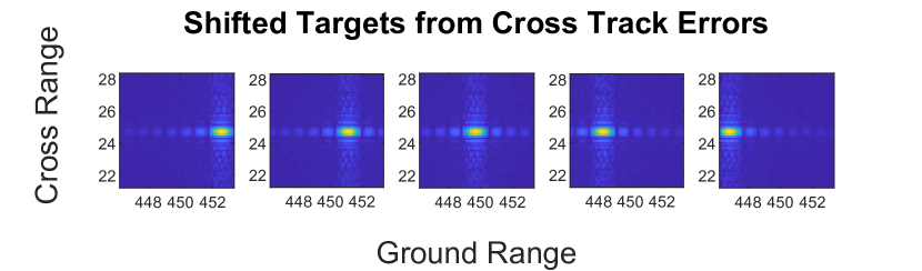
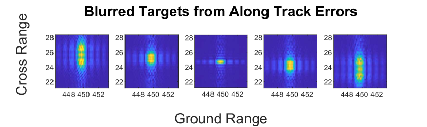
Fig. 1: Demonstration of shifting and blurring distortions due to navigation errors. (Top) Shift distortions caused by errors in cross track position. From left to right, cross track errors are -3, -1.5, 0, 1.5, and 3 meters. (Bottom) Blur distortions caused by errors in along track velocity. From left to right, along track errors are -0.4, -0.2, 0, 0.2, and 0.4 meters per second.

3 The SAR Data

Three different sets of SAR image data were generated for training and testing: simulated data with a 5 second aperture length (sim-5-sec), and two real datasets with 2 (real-2-sec) and 10 second (real-10-sec) aperture lengths, respectively. Simulated data is generated from flight and radar software developed in MATLAB. The software has the capability to generate a flight trajectory, populate the ground with radar targets, and form both truth and distorted SAR images via the BPA from synthesized radar data [33, 20]. For the real datasets, the radar data is obtained from flight tests of the Space Dynamics Laboratory X-band radar system. A sub-centimeter-accurate, post-processed trajectory is used as truth, and corrupted to synthesize distorted SAR images.

Scenario #	AT Pos	CT Pos	D Pos	AT Vel	CT Vel	D Vel
1	x	x
2				x	x
3	x	x		x	x
4	x	x	x
5				x	x	x
6	x	x	x	x	x	x

Table 2: Summary of scenarios and corresponding initial errors.

For each of the simulated and real datasets, six different scenarios were studied, with varying numbers and combinations of active navigation errors, as shown in Table 2. For each of the six scenarios, a total of 192, 185, and 175 unique target locations were considered for the sim-5-sec, real-2-sec, and real-10-sec dataset, respectively. For each target, we generated 100 distorted images of size $80\times 80$ pixels, paired with the corresponding navigation errors. The datasets were then sorted by targets into training, validation, and testing sets as shown in Table 3. We train on a set of targets, and validate and test on an entirely different set of targets. Thus a network’s performance on the test dat reflects its ability to generalize to new locations.

Dataset	Training		Validation		Testing
	# targets	# images	# targets	# images	# targets	# images
Sim-5-sec	134	13500	19	1900	39	3800
Real-2-sec	130	13000	18	1800	37	3700
Real-10-sec	122	12300	17	1700	36	3500

Table 3: Data split details. The six datasets of the sim-5-sec, real-2-sec, and real-10-sec data were approximately split into a $70\%$ training, $10\%$ validation, and $20\%$ testing set.

The brightness of each pixel of a SAR image represents the reflectivity of all targets within that pixel’s region. The intensities of the pixels are inherently right-skewed and subject to changes in magnitude based on the geometric conditions. Thus, we preprocessed the images and errors as follows.

Let $X$ be an input image, $X^{\prime}$ the corresponding reference image, and $y_{\alpha_{\beta}}$ the corresponding navigational error vector. We first log-transform each pixel in each image (including the reference images): $L=\log_{10}(X)$ as is common practice in SAR images. We then standardize each pixel in the image to ensure standardized inputs to the neural network by subtracting the mean and dividing by the standard deviation: $Z=\frac{L-\mu_{L}}{\sigma_{L}}$, where $\mu_{L}$ and $\sigma_{L}$ are estimated on an image-by-image basis.

Each of the navigational errors $y_{\alpha_{\beta}}$ are measured on different scales. We therefore standardize the navigational errors as $\bm{s}=\frac{\bm{y}-\mu_{\bm{y}}}{\sigma_{\bm{y}}}$ to ensure equal consideration of all navigational errors during training. We estimate $\mu_{\bm{y}}$ and $\sigma_{\bm{y}}$ from the entire dataset. In practice, the standardization of the navigation parameters would use a mean of 0 (assuming unbiased navigation errors on average) and a standard deviation estimated from a extended Kalman filter [34].

4 Neural Network Methods

Convolutional neural networks (CNN) are a special case of a neural network that achieve very good performance on image recognition tasks [35, 36, 37]. We therefore use CNN architectures to learn the initial navigational errors. We considered multiple ResNet [35] and Wide ResNet [38] architectures. Each of these architectures is built with the residual block. This block allows networks to be much deeper (more layers and hence better at dealing with images) while simultaneously mitigating the issue of the vanishing gradient [35].

Each of the ResNet and Wide ResNet architectures have pre-trained models trained on large image datasets. We settled on the Wide ResNet 50_2 network because it outperformed all other models, and because its wide (and relatively shallow) nature enables faster training. Our input consists of a 3-channel image with the distorted image, the reference image, and the difference image as each of the channels. This is fed into a randomly initialized convolutional layer followed by the ResNet architecture. The final layer of ResNet is replaced with a fully connected layer with the same number of outputs as error states. In our experiments, we found that fine-tuning all of the ResNet weights resulted in better performance than “freezing” any of the weights or randomly initializing them. This is remarkable considering the datasets used for pretraining contained natural images, which differ considerably from SAR images. This suggests that the pretrained network has learned image features (e.g. lines and other shapes) that are also present in SAR images.

We considered two main approaches for training for the real data. In the first, we simply trained on the real data using the split described in Table 3. In the second, we used transfer learning. Transfer learning is a technique that can help to improve the learning in a new task through the transfer of knowledge from another related task. For example, using the pretrained Wide ResNet 50_2 is a form of transfer learning. The goal of using transfer learning is to fully learn the target task given the transferred knowledge instead of learning from scratch. It can often speed up the training and improve the performance of the model. To do transfer learning in this approach, we pretrained the network (which was already pretrained on other image data) on the simulated training data and then trained on the real training data. The goal of this study was to determine if training on simulated data can improve the performance on real data.

We used the average mean squared error (MSE) loss function across all considered initial errors for training and for testing:

$$\text{MSE}=\frac{1}{mn}\sum_{\alpha=1}^{n}\sum_{\beta=1}^{m}\left(s_{\alpha_{\beta}}-\hat{s}_{\alpha_{\beta}}\right)^{2},$$

where $m$ is the number of error states considered, $n$ is the number of training images in the data, $s_{\alpha_{\beta}}$ is the true standardized error of the $\beta$th error and the $\alpha$th image, and $\hat{s}_{\alpha_{\beta}}$ is the corresponding error estimate by the neural network. The MSE for any prediction can be compared against the value of 1: if the network guesses that the initial error state is 0 or randomly guesses with a mean 0 and a similar standard deviation, then the network will have an estimated MSE of 1. Thus this serves as a benchmark for learning, where an MSE less than one indicates that the neural network is learning relevant information for this task.

5 Experimental Results

Table 4 lists the results obtained in all six scenarios for both the sim-5-sec and the real-2-sec dataset. For all scenarios in the simulated dataset, the MSE is less than $1$ for all considered errors. In particular, the simulated dataset performs well for scenarios 1 and 2, where no ambiguity exists. These results suggest that the neural network is capable of characterizing both shifts and blurs, in the absence of ambiguity. However, as more errors are introduced, the performance degrades, suggesting difficulties in resolving ambiguous error sources.

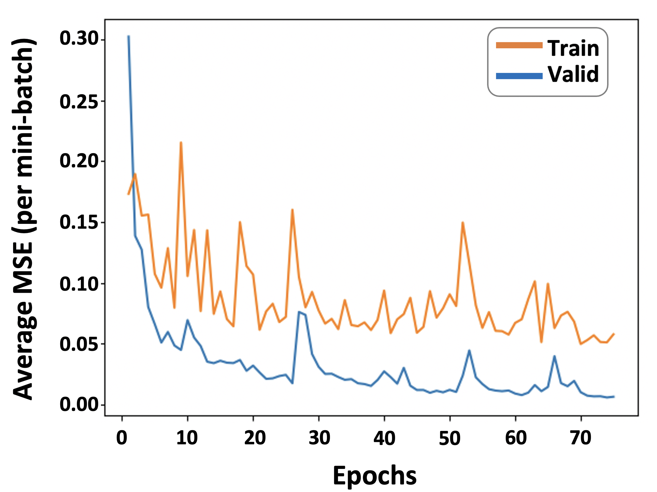
Fig. 2: Training and validation MSE as a function of training epoch for scenario 1. The gap between the errors is small.

In the real dataset, the MSE is below 1 for all errors in scenarios 1 and 4. The network performs particularly well in scenario 1 with a low MSE (see also Figure 2). It is noteworthy that for scenario 4, ambiguity exists in CT shifts, due to either CT or D position errors. The network, however, is able to identify subtleties in the distorted SAR images and properly attribute the effect to the corresponding error. Figure 3 shows the distribution of the error states before and after estimation of the navigation errors for scenarios 1 and 4. The resulting error distributions are more concentrated around zero, indicating that the neural network is able to improve our knowledge of the initial error states. Furthermore, no outliers are introduced by the neural network. However, as was the case for the simulated dataset, increasing numbers of ambiguous error sources results in degraded overall performance, with an MSE near 1.0 in cases where little information is learned by the network.

Scenario #	Dataset	AT Pos	CT Pos	D Pos	AT Vel	CT Vel	D Vel
1	MSE (Sim-5-sec)	0.0594	0.0289	N/A	N/A	N/A	N/A
	MSE (Real-2-sec)	0.0563	0.0425	N/A	N/A	N/A	N/A
2	MSE (Sim-5-sec)	N/A	N/A	N/A	0.2456	0.1162	N/A
	MSE (Real-2-sec)	N/A	N/A	N/A	1.0729	0.1683	N/A
3	MSE (Sim-5-sec)	0.5229	0.2237	N/A	0.2442	0.1259	N/A
	MSE (Real-2-sec)	1.0657	0.2340	N/A	1.0682	0.1468	N/A
4	MSE (Sim-5-sec)	0.0941	0.9204	0.2800	N/A	N/A	N/A
	MSE (Real-2-sec)	0.1020	0.8102	0.3734	N/A	N/A	N/A
5	MSE (Sim-5-sec)	N/A	N/A	N/A	0.2834	0.7982	0.5460
	MSE (Real-2-sec)	N/A	N/A	N/A	1.0699	0.6459	0.5795
6	MSE (Sim-5-sec)	0.6321	0.9139	0.5245	0.3677	0.8661	0.5331
	MSE (Real-2-sec)	1.0846	0.7509	0.5353	1.0868	0.6039	0.5984

Table 4: Summary of Model Performance for each error state for scenarios 1-6 of the sim-5-sec and the real-2-sec datasets. The network is able to learn many of the errors for both simulated and real data ($MSE<1$).

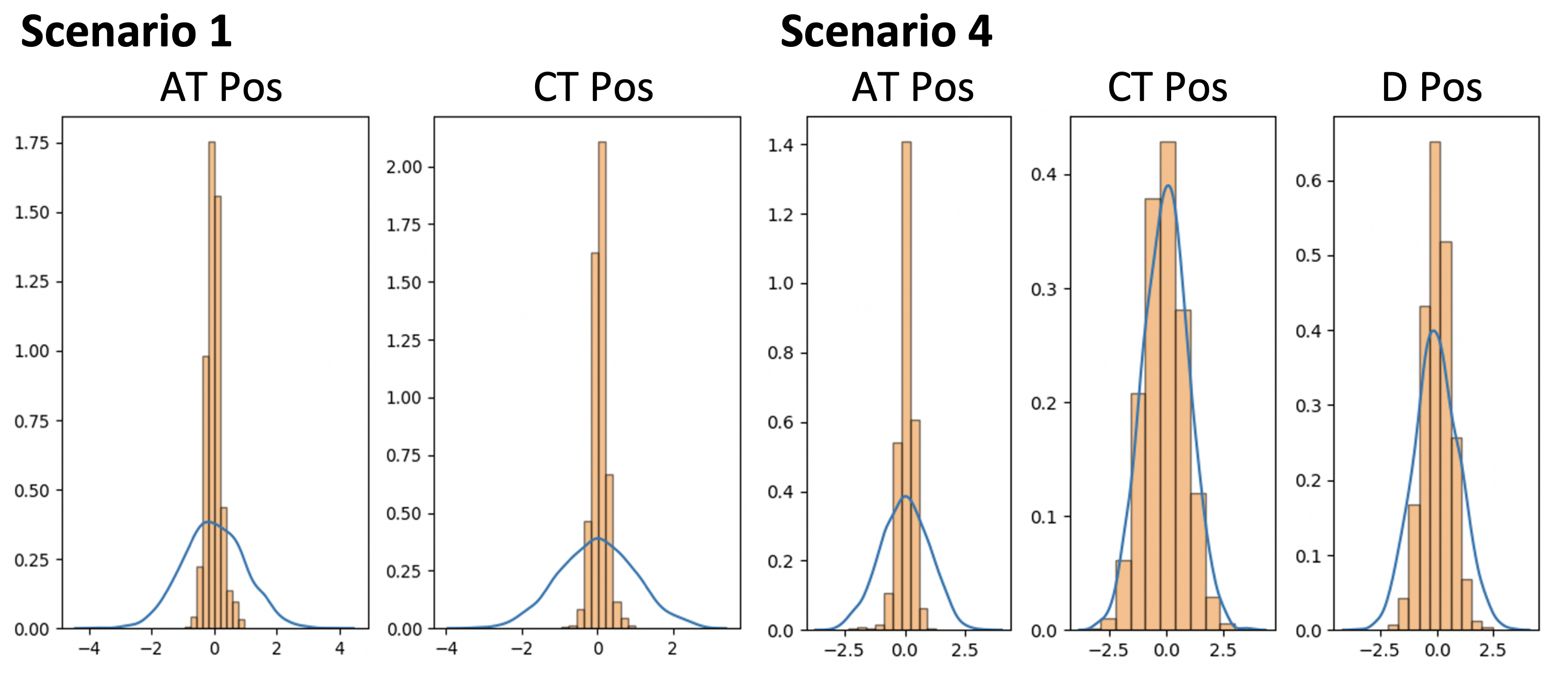
Fig. 3: Distribution of Error States before (blue line) and after (histogram) estimation for the real-2-sec dataset for scenarios 1 and 4. In both cases, the error distributions are more concentrated around zero, indicating that the network has improved our ability to estimate navigation errors. No outliers have been introduced by the network.

For some of these errors, the network may also be overfitting. Figure 4 shows the training and validation MSE as a function of training epoch for scenario 2. Here, we see that the average training error is very low, indicating that the network is able to accurately predict both errors on the training set. However, the validation MSE is considerably higher, suggesting that overfitting is occurring. Increasing the amount of training data, especially adding more targets, will likely reduce the tendency to overfit.

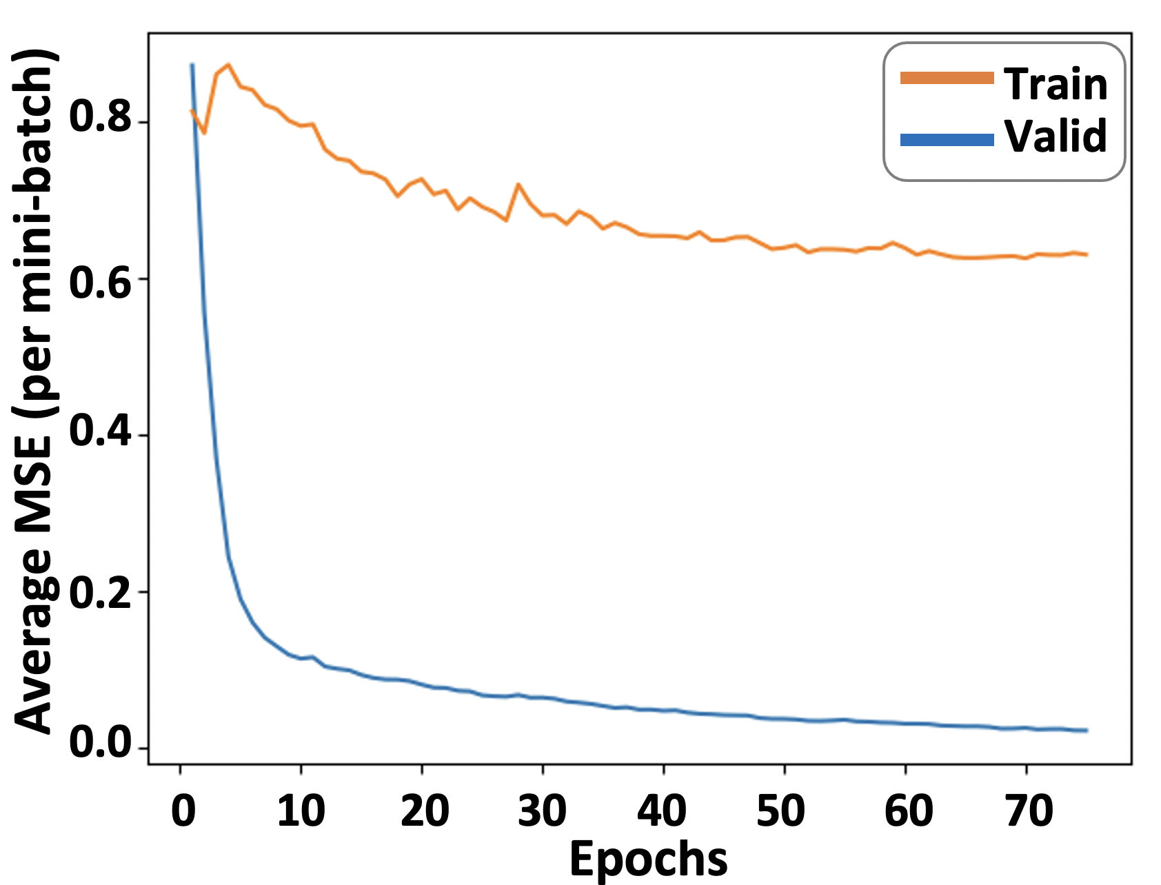
Fig. 4: Training and validation MSE as a function of training epoch for scenario 2 for the real-2-sec dataset. There is a large gap between the training and validation error, suggesting the network may be overfitting. Compare with Figure 2 where little overfitting is occurring in scenario 1.

As observed in scenario 2 of the real-2-sec dataset, the network was not able to characterize blur distortions for the 2-second synthetic aperture despite the lack of error ambiguity. Table 5 summarizes the network’s performance in this scenario for a 2-second aperture, as compared to a 10-second aperture. In the latter case, the MSE for the North velocity error decreased by more than 25%, suggesting that the neural network successfully characterized the effect of blurs for the larger apertures. Notably, the neural network also improves its estimation of the East velocity error by a factor of 2. These results identify a trend of improved performance on real datasets with increasing aperture length.

Dataset, Scenario 2	AT Vel	CT Vel
MSE (Real-2-sec)	1.0729	0.1683
MSE (Real-10-sec)	0.7895	0.0812
MSE (Transfer Learning - 2 sec)	1.0429	0.0849

Table 5: Summary of Model Performance for the error states present in scenario 2. This table shows: 1) the results of applying the proposed model on the real-2-sec and real-10-sec data; 2) the results of pretraining on simulated data and training on real-2-sec data. Going from 2 seconds to 10 seconds improves the performance. Improvements from transfer learning are negligible.

We also applied transfer learning, where we trained the network on the sim-5-sec dataset first, then trained on the real-2-sec dataset. Table 5 shows the performance for scenario 2. We see that transfer learning resulted in negligible improvement in both the AT and CT velocity MSE. Similar results were obtained in other scenarios.

6 Conclusion

We used a convolutional neural network to estimate position and velocity errors at the beginning of a SAR data collection period, by comparison of a distorted SAR image to an a priori SAR reference image. Performance was assessed on both simulated and real SAR data. In general, the network performs well in the absence of ambiguous error sources, reducing the MSE of the active navigation errors. As the number of error sources increases, the performance degrades due to the inability to separate errors which result in the same image distortion. In the case of the real data, however, the network successfully separated CT shifts caused by CT and D position errors. This exciting result suggest that the network is able to identify subtleties in the image distortions that are not readily apparent to human eyes. Another key finding in the testing of the network on real data, is sensitivity of estimation performance on the length of the synthetic aperture. As the length increases, the network successfully characterizes blurring in real images, and appropriately attributes it to the corresponding error source.

Future work includes further investigation of the effect of the aperture length on the network’s ability to learn. Furthermore, the sensitivity of distortions to the vehicle/target geometry may be exploited to reduce ambiguities and improve performance. Future approaches may, therefore, augment the training data with information about the viewing geometry, including the estimated vehicle position at the beginning/end of the synthetic aperture, the location of known targets, or the time history of barometric altimeter measurements. Finally, including more training data in future iterations will likely help mitigate overfitting.

References

- [1] J. Raquet and R. K. Martin, “Non-GNSS radio frequency navigation,” in ICASSP, Mar. 2008, pp. 5308–5311.
- [2] M. J. Veth, “Navigation Using Images, A Survey of Techniques,” Navigation, vol. 58, no. 2, pp. 127–139, 2011.
- [3] E. B. Quist, P. C. Niedfeldt, and R. W. Beard, “Radar odometry with recursive-RANSAC,” IEEE Trans. Aerosp. Electron. Syst., vol. 52, no. 4, pp. 1618–1630, Aug. 2016.
- [4] E. B. Quist and R. W. Beard, “Radar odometry on fixed-wing small unmanned aircraft,” IEEE Trans. Aerosp. Electron. Syst., vol. 52, no. 1, pp. 396–410, Feb. 2016.
- [5] A. F. Scannapieco, A. Renga, G. Fasano, and A. Moccia, “Experimental Analysis of Radar Odometry by Commercial Ultralight Radar Sensor for Miniaturized UAS,” J. Intell. Robot. Syst, vol. 90, no. 3-4, pp. 485–503, June 2018.
- [6] P. Samczynski and K.S. Kulpa, “Coherent MapDrift Technique,” IEEE Trans. Geosci. Remote Sens, vol. 48, no. 3, pp. 1505–1517, Mar. 2010.
- [7] P. Samczynski, “Superconvergent Velocity Estimator for an Autofocus Coherent MapDrift Technique,” IEEE Geosci. Remote Sense. Lett, vol. 9, no. 2, pp. 204–208, Mar. 2012.
- [8] L. Hostetler and R. Andreas, “Nonlinear Kalman filtering techniques for terrain-aided navigation,” IEEE Trans. Automat. Contr, vol. 28, no. 3, pp. 315–323, Mar. 1983.
- [9] J. Hollowell, “Heli/SITAN: a terrain referenced navigation algorithm for helicopters,” in PLANS, Mar. 1990, pp. 616–625.
- [10] N. Bergman, L. Ljung, and F. Gustafsson, “Terrain navigation using Bayesian statistics,” IEEE Control Syst. Mag, vol. 19, no. 3, pp. 33–40, June 1999.
- [11] P.-J. Nordlund and F. Gustafsson, “Marginalized Particle Filter for Accurate and Reliable Terrain-Aided Navigation,” IEEE Trans. Aerosp. Electron. Syst., vol. 45, no. 4, pp. 1385–1399, Oct. 2009.
- [12] Y Kim, J Park, and H Bang, “Terrain-Referenced Navigation using an Interferometric Radar Altimeter: IRA-Based TRN,” Navigation, vol. 65, no. 2, pp. 157–167, June 2018.
- [13] Z Sjanic and F Gustafsson, “Simultaneous navigation and SAR auto-focusing,” in FUSION, July 2010, pp. 1–7.
- [14] M. Greco, S. Querry, G. Pinelli, K. Kulpa, P. Samczynski, D. Gromek, A. Gromek, M. Malanowski, B. Querry, and A. Bonsignore, “SAR-based augmented integrity navigation architecture,” in IRS, May 2012, pp. 225–229.
- [15] D Nitti, F Bovenga, M Chiaradia, M Greco, and G Pinelli, “Feasibility of Using Synthetic Aperture Radar to Aid UAV Navigation,” Sensors, vol. 15, no. 8, pp. 18334–18359, July 2015.
- [16] E. C. Zaugg and D. G. Long, “Generalized Frequency Scaling and Backprojection for LFM-CW SAR Processing,” IEEE Trans. Geosci. Remote Sens, vol. 53, no. 7, pp. 3600–3614, July 2015.
- [17] W. G. Carrara, R. S. Goodman, and R.d M. Majewski, Spotlight SAR: Signal processing algorithms, Artech House, Boston, 1995.
- [18] F Ulaby and D Long, Microwave Radar and Radiometric Remote Sensing, University of Michigan Press, Ann Arbor, 2014.
- [19] R. S. Christensen, J. Gunther, and D. Long, “Toward gps-denied navigation utilizing back projection-based synthetic aperture radar imagery,” in Proceedings of the ION 2019 Pacific PNT Meeting, 2019, pp. 108–119.
- [20] C. Lindstrom, R. Christensen, and J. Gunther, “Sensitivity of bpa sar image formation to initial position, velocity, and attitude navigation errors,” arXiv, vol. abs/2009.10210, 2020.
- [21] V Berisha, N Shah, D Waagen, H Schmitt, S Bellofiore, A Spanias, and D Cochran, “Sparse manifold learning with applications to sar image classification,” in ICASSP. IEEE, 2007, vol. 3, pp. III–1089.
- [22] S Chen and H Wang, “Sar target recognition based on deep learning,” in DSAA. IEEE, 2014, pp. 541–547.
- [23] S Chen, H Wang, F Xu, and Y.-Q. Jin, “Target classification using the deep convolutional networks for sar images,” IEEE Trans. Geosci. Remote Sens, vol. 54, no. 8, pp. 4806–4817, 2016.
- [24] M Wilmanski, C Kreucher, and J Lauer, “Modern approaches in deep learning for sar atr,” in Algorithms for SAR imagery, 2016, vol. 9843, p. 98430N.
- [25] Q Zhao and J. C. Principe, “Support vector machines for sar automatic target recognition,” IEEE Trans. Aerosp. Electron. Syst., vol. 37, no. 2, pp. 643–654, 2001.
- [26] B Krishnapuram, D Williams, Y Xue, L Carin, M Figueiredo, and A. J. Hartemink, “On semi-supervised classification,” in NeurIPS, 2005, pp. 721–728.
- [27] M Gong, J Zhao, J Liu, Q Miao, and L Jiao, “Change detection in synthetic aperture radar images based on deep neural networks,” IEEE Trans. Neural Netw. Learn. Syst, vol. 27, no. 1, pp. 125–138, 2016.
- [28] E Mason, B Yonel, and B Yazici, “Deep learning for radar,” in RadarConf. IEEE, 2017, pp. 1703–1708.
- [29] A. O. Hero, B. Ma, O. JJ. Michel, and J. Gorman, “Applications of entropic spanning graphs,” IEEE Signal Process. Mag, vol. 19, no. 5, pp. 85–95, 2002.
- [30] M. E. Tipping and C. M. Bishop, “Bayesian image super-resolution,” in NeurIPS, 2003, pp. 1303–1310.
- [31] L. C. Pickup, D. P. Capel, S. J. Roberts, and A. Zisserman, “Bayesian image super-resolution, continued,” in NeurIPSs, 2007, pp. 1089–1096.
- [32] M. V. Wyawahare, P. M. Patil, H. K. Abhyankar, et al., “Image registration techniques: an overview,” Int. J. Signal Process. Image Process. and Patt. Recog, vol. 2, no. 3, pp. 11–28, 2009.
- [33] M. I. Duersch and D. G. Long, “Analysis of time-domain back-projection for stripmap SAR,” International Journal of Remote Sensing, vol. 36, no. 8, pp. 2010–2036, Apr. 2015.
- [34] R. E. Kalman, “A new approach to linear filtering and prediction problems,” J. Basic Eng, vol. 82, no. 1, pp. 35–45, 1960.
- [35] K. He, X. Zhang, S. Ren, and J. Sun, “Deep residual learning for image recognition,” in CVPR, 2016, pp. 770–778.
- [36] A. Krizhevsky, I. Sutskever, and G. E. Hinton, “Imagenet classification with deep convolutional neural networks,” in NeurIPS, 2012, pp. 1097–1105.
- [37] T. N. Sainath, A.-r. Mohamed, B. Kingsbury, and B. Ramabhadran, “Deep CNN for LVCSR,” in ICASSP. IEEE, 2013, pp. 8614–8618.
- [38] S. Zagoruyko and N. Komodakis, “Wide residual networks,” arXiv, vol. abs/1605.07146, 2016.