ROGER: Reconstructing Orbits of Galaxies in Extreme Regions using machine learning techniques

Abstract

We present the ROGER (Reconstructing Orbits of Galaxies in Extreme Regions) code, which uses three different machine learning techniques to classify galaxies in, and around, clusters, according to their projected phase-space position. We use a sample of 34 massive, $M_{200}>10^{15}h^{-1}M_{\odot}$, galaxy clusters in the MultiDark Planck 2 (MDLP2) simulation at redshift zero. We select all galaxies with stellar mass $M_{\star}\geq 10^{8.5}h^{-1}M_{\odot}$, as computed by the semi-analytic model of galaxy formation SAG, that are located in, and in the vicinity of, these clusters and classify them according to their orbits. We train ROGER to retrieve the original classification of the galaxies from their projected phase-space positions. For each galaxy, ROGER gives as output the probability of being a cluster galaxy, a galaxy that has recently fallen into a cluster, a backsplash galaxy, an infalling galaxy, or an interloper. We discuss the performance of the machine learning methods and potential uses of our code. Among the different methods explored, we find the K-Nearest Neighbours algorithm achieves the best performance.

1 Introduction

Galaxies in the Universe show a wide variety of properties as a result of the action of both, internal and environmental processes. Clusters of galaxies constitute the most extreme environments in the Universe for galaxy evolution. They are the most massive objects $(\sim 10^{14-15}M_{\odot})$ in virial equilibrium, are characterised by a deep gravitational potential well, a large number of galaxy members, and an intracluster medium filled with hot ionised gas. Galaxies in clusters exhibit different properties compared to galaxies that reside in the field, or in less massive systems.

Several physical processes affect galaxies inside clusters in a simultaneous way. One of these mechanisms is the ram pressure stripping (e.g. Gunn & Gott 1972; Abadi et al. 1999; Book & Benson 2010; Steinhauser et al. 2016). This process can remove an important fraction of the cold gas from galaxies, resulting in the inhibition of star formation. Although this mechanism is more effective at the central regions of massive clusters, it has been reported in less massive systems (e.g. Rasmussen et al. 2006; Jaffé et al. 2012; Hess & Wilcots 2013). Ram pressure stripping occurs as galaxies move at high speeds through the hot ionised gas of the intracluster medium, which collides with the cold gas of the galaxies and removes it. The warm gas from the galactic halo can also be removed by the gas of the intracluster medium, a process known as starvation (e.g. Larson et al. 1980; Balogh et al. 2000; McCarthy et al. 2008; Bekki 2009; Bahé et al. 2013; Vijayaraghavan & Ricker 2015). This process can cut off further gas cooling from the galaxy’s halo gas that fuels future star formation. Kawata & Mulchaey (2008) predicted that starvation can act in galaxy groups as well. Another physical process that works on galaxies in their passage through the deep potential well of the cluster is tidal stripping (e.g. Zwicky 1951; Gnedin 2003a; Villalobos et al. 2014). It can induce a central star formation burst (Byrd & Valtonen, 2001), bar instabilities (Łokas et al., 2016), changes in the pattern of the spiral arms (Semczuk et al., 2017), and truncate dark matter haloes (e.g. Gao et al. 2004; Limousin et al. 2009). In the outskirts of clusters, mechanisms like galaxy-galaxy interaction, known as harassment, are more effective (e.g. Moore et al. 1996; Moore et al. 1998; Gnedin 2003b; Smith et al. 2015). Most of the processes mentioned above tend to decrease or to completely suppress the star formation in galaxies. As a consequence, galaxies in clusters are typically red, early-type, with an old stellar population, and have little or none star formation at all.

Clusters of galaxies are continually accreting galaxies. Some galaxies may fall as members of galaxy groups and, therefore, they may have already experienced environmental effects that accelerated the consumption of their gas reservoir prior to entering the cluster. This is known as pre-processing (e.g. Mihos 2004; Fujita 2004), and has both observational and theoretical support (e.g. Balogh et al. 1999; McGee et al. 2009; De Lucia et al. 2012; Jaffé et al. 2012; Wetzel et al. 2013; Hou et al. 2014). In the outskirts of clusters, not only star forming and pre-processed galaxies are found, but also backsplash galaxies. These are galaxies that have orbited the central regions of the cluster only once since their infall. They are currently outside the cluster, and will fall back to the cluster in the future (e.g. Gill et al. 2005; Rines & Diaferio 2005; Aguerri & Sánchez-Janssen 2010; Muriel & Coenda 2014). Backsplash galaxies do not necessarily have become passive yet. They have suffered the extreme environmental effects of the inner regions of a cluster, which has surely left traces in their physical properties. Consequently, the characterisation of this population of galaxies is important to understand the effects that the cluster environment produces in galaxies.

Since the efficiency of the physical processes described above depends heavily on the history of galaxies in and around clusters, a detailed knowledge of galaxy orbits is essential. It is customary to classify galaxies around clusters using different criteria according to their position in the Projected Phase-Space Diagram (PPSD). This two-dimensional space combines the projected cluster-centric distance, with the line-of-sight velocity relative to the cluster. Oman et al. (2013) use a N-body simulation to compile a catalogue of the orbits of satellite haloes in cluster environments. They found that satellite haloes in different phases of their orbits occupy different regions in the PPSD. Mahajan et al. (2011) quantify the decrease of star formation in backsplash galaxies. Muzzin et al. (2014) find that quiescent, star forming and post-starburst galaxies in clusters at $z\sim 1$, are distributed differently in the PPSD. Muriel & Coenda (2014) study the properties of galaxies in the outskirts of a sample of 90 galaxy clusters. They split galaxies into two classes: those with high relative velocity, and those with low relative velocity, being the latter candidates to be backsplash galaxies. These authors find that backsplash candidates are systematically older, redder, and have formed fewer stars in the last 3 Gyrs than high-velocity galaxies. In addition, Hernández-Fernández et al. (2014) and Jaffé et al. (2015) infer the orbital histories of cluster galaxies from their PPSD positions to investigate the effects of ram pressure on the gas fraction of galaxies. Oman & Hudson (2016) measure quenching time-scales in clusters as a function of the position in the PPSD. Yoon et al. (2017) trace the gas stripping histories of galaxies infalling into the Virgo cluster using a reference sample in the PPSD. Jaffé et al. (2018) reconstruct the stripping history of jellyfish galaxies using their PPSD position as an indication of their orbits.

Using cosmological hydrodynamic N-body simulations of groups and clusters, Rhee et al. (2017) separate galaxies in the PPSD as a function of the time elapsed since their infall into the system: first, recent, intermediate, and ancient infallers. They define regions in the PPSD where each of these types of galaxies are more likely to be found. These regions can, in turn, be used to classify galaxies from their PPSD position. An alternative tool is given by Pasquali et al. (2019). They use cosmological simulations of groups and clusters and derive zones of constant mean infall time. They use these zones to study the environmental effects upon satellite galaxies. They provide an analytical form for the curves that define each zone. Smith et al. (2019) use these zones in the PPSD to create samples of ancient and recent infallers among satellite galaxies in a SDSS group catalogue. They use these samples to study the stellar mass growth histories of galaxies as a function of infall time.

Although many interesting results have been obtained using the PPSD, in practice it is very difficult to determine with certainty whether a particular galaxy is a backsplash, or it is infalling to the cluster for the first time, or if it has already become a cluster member. In this work we take a different approach by classifying galaxies relating their three-dimensional orbits with their position in the PPSD. We use a sample of massive clusters from the MultiDark Planck 2 (MDLP2) cosmological simulation (Klypin et al., 2016) and generate the galaxy population with the semi-analytic model of galaxy formation SAG (Cora et al., 2018). We classify galaxies in and around these clusters into five types, according to their three-dimensional orbits. Then, we develop a Machine Learning code and train it to recover the orbital classification (3-D) of the galaxies out of their PPSD position (2-D). Machine learning techniques represent a new way of analysing big data-sets in an agnostic and homogeneous way. Taking into account the amount of data generated by current and future surveys and simulations, the data-driven techniques will become a fundamental tool for their analysis. These methods are very useful and powerful tools to find patterns and relations between the variables that are involved in a specific problem. In particular, these methods are especially good in classification problems (de los Rios et al., 2016; Bom et al., 2017; Diaz Rivero & Dvorkin, 2020).

This article is organised as follows: we describe the data sets of simulated clusters and galaxies in Sect. 2, where we also define different galaxy types according to their orbits; in sect. 3, we present our code ROGER (Reconstructing Orbits of Galaxies in Extreme Regions) that relates the two-dimensional PPSD position of galaxies to their 3-D orbits, and analyse its performance; finally, we present our conclusions in Sect. 4.

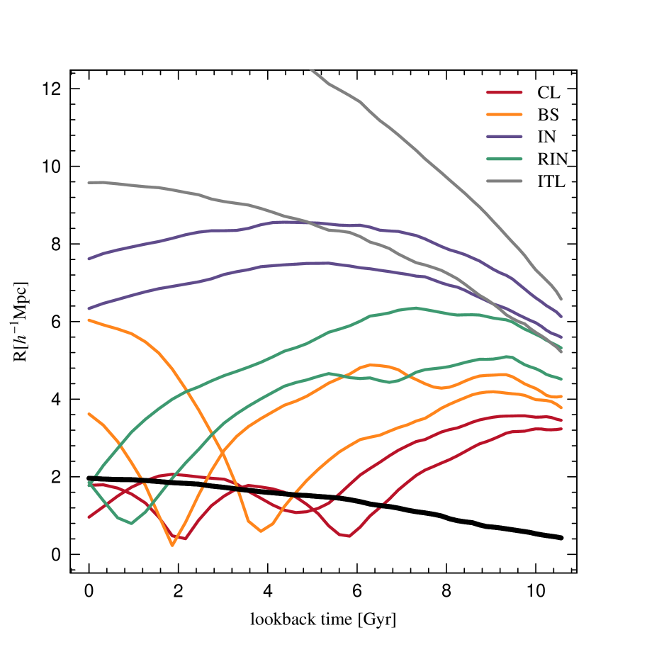
Figure 1: Cluster-centric distance as a function of lookback time for ten galaxies in/around one of the clusters in our sample. The thick black solid line represents the $R_{200}$ of the cluster. Different colours correspond to galaxies classified as: cluster members (CL, red lines), recent infallers (RIN, green lines), backsplash (BS, orange lines), infall galaxies (IN, violet lines), and interlopers (ITL, gray lines).

2 The sample of simulated clusters and galaxies

We use a sample of clusters and galaxies from a simulated galaxy catalogue constructed using the semi-analytic model of galaxy formation and evolution SAG (Semi-Analytic Galaxies, Cora et al. 2018). As a backbone for this synthetic catalogue, we use dark matter haloes and subhaloes, and their corresponding merger trees, extracted from the cosmological simulation MDPL2 (Klypin et al., 2016). In this section, we briefly present the MDPL2 simulation and the SAG code, and describe the samples of simulated clusters and galaxies we use throughout the paper.

2.1 The MDPL2 simulation

The MDPL2 simulation is part of the MultiDark suite of dark matter simulations, publicly available at the CosmoSim database (Riebe et al., 2013; Klypin et al., 2016). The simulation has $3840^{3}$ dark matter particles in a comoving cubic volume of $1~{}h^{-3}{\rm Gpc^{3}}$, evolved from redshift 120 to redshift 0. The cosmology adopted corresponds to a $\Lambda$CDM model with parameters consistent with Planck measurements (Planck Collaboration et al., 2014, 2016): $\Omega_{\rm m}=0.307$, $\Omega_{\rm\Lambda}=0.693$, $\Omega_{\rm b}=0.048$, $\sigma_{8}=0.823$, $n=0.96$, and $h=0.678$. Dark matter haloes were identified using the Rockstar halo finder (Behroozi et al., 2013a), keeping all the dark matter bounded structures with at least 20 particles. The final catalogue comprises $\sim 127\times 10^{6}$ haloes, whose merger trees were constructed using the ConsistentTrees algorithm (Behroozi et al., 2013b).

2.2 The SAG model

The version of SAG used in this work was presented in detail in Cora et al. (2018). This model includes the main physical processes relevant to galaxy formation and evolution: radiative cooling of hot gas in central and satellite galaxies, star formation in quiescent and bursty modes, being the latter triggered by galaxy mergers and disc instabilities, detailed treatment of chemical enrichment of gaseous and stellar components, supernova feedback and stellar winds, gas ejection and reincorporation of hot gas, central super-massive black hole growth and AGN feedback, ram pressure and tidal stripping. For a complete and detailed description of all of these processes and their implementations, we refer the reader to Cora (2006), Lagos et al. (2008), Tecce et al. (2010), Gargiulo et al. (2015), Muñoz Arancibia et al. (2015), Ruiz et al. (2015), Cora et al. (2018), Collacchioni et al. (2018), and Cora et al. (2019).

2.3 Galaxies in and around clusters in the MDPL2-SAG catalogue

From the MDPL2 simulated volume, we select all haloes at redshift zero that have a mass, computed within the region that encloses 200 times the critical density, $M_{\rm 200}\geq 10^{15}h^{-1}M_{\odot}$. Furthermore, we impose an isolation criterion by requiring that they have no companion haloes more massive than $0.1\times M_{\rm 200}$, within $5\times R_{\rm 200}$, where $R_{\rm 200}$ is the radius enclosing the overdensity. With this restriction, we exclude from our analysis haloes undergoing a major merger, or interacting with a massive companion. Both these situations are likely to affect galaxy orbits to a great extent in the vicinity of the main halo. Out of the 85 haloes more massive than $10^{15}h^{-1}M_{\odot}$ in the MDPL2 volume, our selection results in a set of 34 massive, relaxed haloes that constitute our cluster sample for the present paper.

In order to guarantee completeness, we impose a low stellar mass cut-off of $\log_{10}(M_{\star}^{\rm min}/h^{-1}M_{\odot})=8.5$ in our sample of galaxies (Knebe et al., 2018). Below this mass limit, observed stellar mass functions are not well reproduced and galaxy properties are not followed in a reliable way.

For each cluster in our sample, we follow the trajectory of all central galaxies and of those satellite galaxies that keep their dark matter substructure and that end up in a region that includes the cluster and its surroundings. We choose each of these regions to be a cylinder elongated along the $z-$axis of the simulation box to include not only the cluster galaxies and galaxies in the surroundings of the cluster, but also interlopers, i.e., galaxies that will appear in or around the cluster in projection but are unrelated to it; interlopers constitute the main source of contamination in the PPSD. There is no lost of generality by choosing cylinders parallel to the $z-$axis, i.e., we are choosing the line-of-sight direction to be this axis of the simulation box. The dimensions of these cylinders are: a radius of $5\times R_{\rm 200}$, and a longitude in the $z-$axis that extends as far as to include all galaxies within $|\Delta V_{z}+H_{0}\Delta z|\leq 3\sigma$, where $\Delta V_{z}$ is the galaxy peculiar velocity in the $z$ direction relative to the cluster, $\Delta z$ is the proper distance between the galaxy and the cluster in the $z-$direction, $H_{0}=67.8\,{\rm km}\,{\rm s}^{-1}\,{\rm Mpc}^{-1}$ is the Hubble constant, and $\sigma$ is the one dimensional velocity dispersion of the cluster. As shown by Munari et al. (2013), the measurement of $\sigma$ produces different values depending on whether dark matter particles or subhaloes are used in the computation. For consistency, we computed $\sigma$ out of the satellite galaxies more massive than $M_{\star}^{\rm min}$, using the biweight estimator of Beers et al. (1990). We recall that satellite galaxies in the MDPL2-SAG catalogue are the central galaxies of the subhaloes, thus our estimation of $\sigma$ is made out of those subhaloes that harbor a central galaxy more massive than our chosen stellar mass threshold.

We classify all galaxies in these cylinders into different types according to their orbits around clusters. These galaxies are, in turn, used to train and test the machine learning algorithms described in the next section. We define five classes of galaxies:

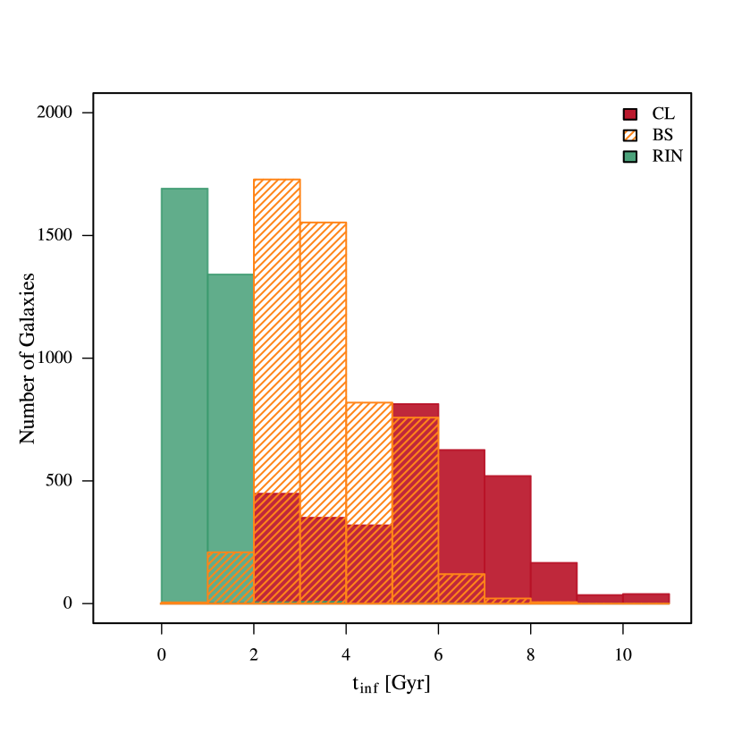
Figure 2: Distribution of the time since first infall for all galaxies in our sample that have been within $R_{\rm 200}$ of a cluster at some point in their lifetimes. Colours are as in Fig. 1.

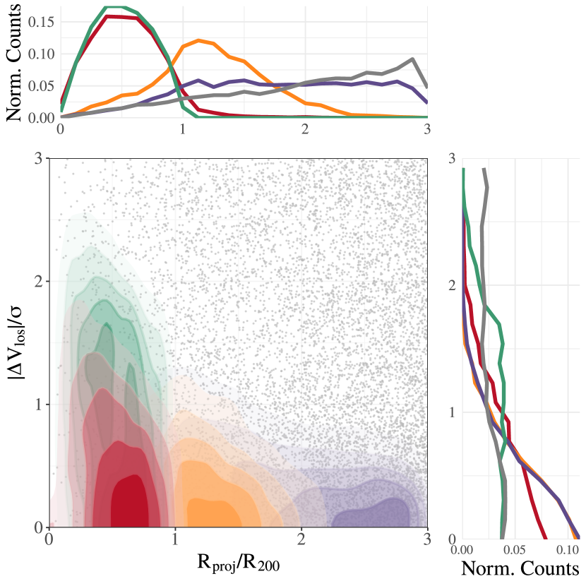
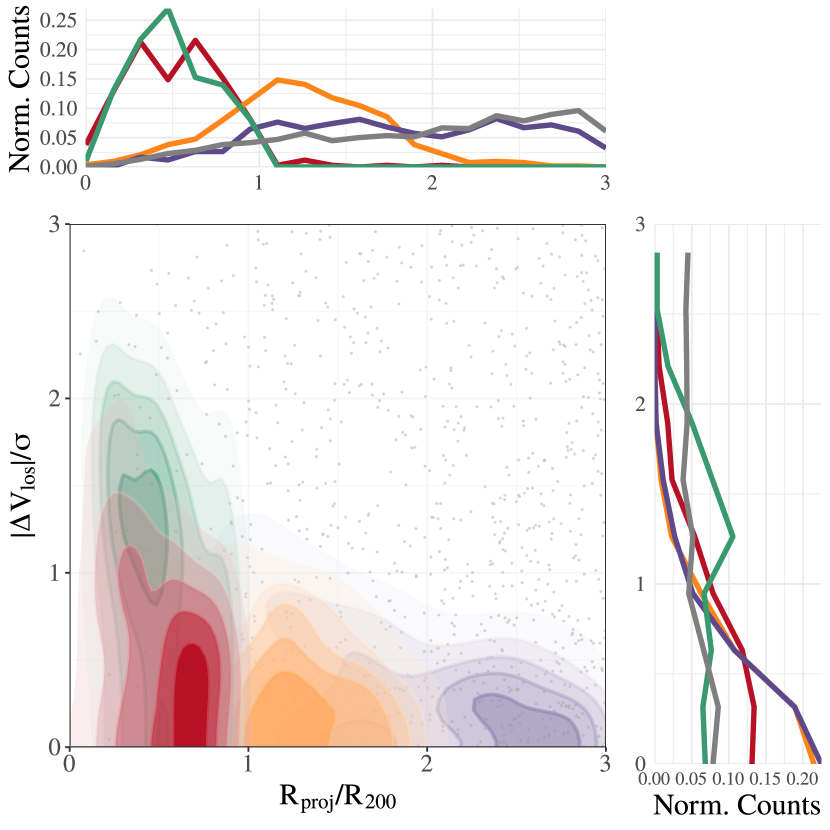
Figure 3: Projected phase-space diagram of our full sample (left panel) and of the validation-set (right panel) of MDPL2-SAG galaxies. In the main box, we show in different colour shades the density of galaxies classified as CL (red), RIN (green), BS (orange), and IN (violet). ITL galaxies are shown as individual gray points for clarity. We show in the upper and right-side panels, the corresponding marginalised distributions of $R_{\rm proj}/R_{200}$ and $|\Delta V_{\rm los}|/\sigma$. These distributions are normalised to have unity area.

1. Clusters members (CL): galaxies that may have crossed $R_{\rm 200}$ several times in the past and now orbit around the cluster centre. Most of them are found within $R_{\rm 200}$ of the cluster centre.

2. Recent infallers (RIN): galaxies that have crossed $R_{\rm 200}$ only once on their way in in the past $2~{}\rm Gyr$ (we discuss the choice of this timescale below). Among these, there are galaxies that can get further away than $R_{\rm 200}$ from the cluster centre in the future.

3. Backsplash galaxies (BS): galaxies that have crossed $R_{\rm 200}$ exactly twice. The first time on their way in, and the second time on their way out of the cluster, where they are found now. Most of these galaxies will fall back into the cluster. Accordingly to this definition, some RIN may become BS in the future.

4. Infalling galaxies (IN): galaxies that have never been closer than $R_{\rm 200}$ to the cluster centre, and their main halo has negative radial velocity relative to the cluster. We consider these galaxies to be either bounded to the cluster, or will potentially fall into the cluster in the future.

5. Interlopers (ITL): galaxies that have never been closer than $R_{200}$ to the cluster centre, but unlike IN, their main halo has a positive radial velocity relative to the cluster, i.e., the halo is receding away from the cluster at redshift zero. In contrast to the IN galaxies described above, we consider these galaxies as objects that will not fall into the cluster. They are galaxies unrelated to the cluster that can be confused with classes (i)-(iv) in the PPSD.

Galaxies of classes (i) to (iv) are of interest in cluster studies, while galaxies of class (v) constitute the main source of contamination at the time of classifying galaxies in and around clusters from an observational point of view.

We show in Fig. 1 examples of how our classification scheme works. For one of the cluster in our sample, we have chosen examples of galaxies from the five classes defined above, and show their three dimensional cluster-centric distance as a function of the lookback time.

Special attention deserves our choice of 2 Gyr to define RIN galaxies above. It makes no sense to classify all galaxies within $R_{\rm 200}$ as cluster members, since some of the galaxies that have entered the clusters in recent times may get out of the cluster in the future, and become BS galaxies. On the other hand, it would be very useful to pick out the galaxies that are experiencing the effects of the cluster environment for the first time. Thus, it is important to define a time-scale to tell apart between ‘old’ cluster galaxies, and galaxies that have fallen into the cluster not a long time ago. When we analysed the distribution of the infall time of galaxies that are within $R_{\rm 200}$ at redshift zero, we find a clear peak at lookback times $t_{\rm inf}\leq 2$ Gyr; this fact motivates our choice of the condition imposed to classify RIN galaxies. We show in Fig. 2 the distribution of the first infall times of galaxies that have been within $R_{\rm 200}$ at least once in their lifetimes, i.e., CL, RIN and BS.

For real galaxies, only their projected distance to the centre of the cluster, and their line-of-sight velocity relative to the cluster can be measured, i.e., their positions in the PPSD. In Fig. 3 (left panel), we show the PPSD of all galaxies in our sample. Phase-space positions of galaxies relative to their parent cluster’s centre are computed by projecting the 3D cartesian coordinates of the galaxies in the MDPL2 box into the $(x,y)$ plane. Hereafter, the projected distance on this plane, $R_{\rm proj}$, will be referred to as the 2D distance, and it will be quoted in units of $R_{200}$ unless otherwise specified. On the other hand, the $z-$axis velocity relative to the cluster, $\Delta V_{\rm los}\equiv|\Delta V_{z}+H_{0}\Delta z|$, will be called the line-of-sight velocity, and will be quoted in units of the velocity dispersion of the cluster, $\sigma$.

As can be seen in Fig. 3, there is much overlap between the five classes of galaxies in the PPSD. Thus, deciding how to classify a galaxy according to its phase-space position is not trivial. CL and RIN galaxies have similar radial distributions, occupying the region defined by $R_{\rm proj}/R_{200}\lesssim 1$. These two classes differ, however, in their line-of-sight velocity distributions: CL galaxies are concentrated towards $\Delta V_{\rm los}/\sigma\sim 0$, while RIN galaxies show a roughly flat distribution up to $\Delta V_{\rm los}/\sigma\sim 1.25$, an indication that the latter do not constitute a population in virial equilibrium. BS galaxies are found preferentially between $0.5R_{200}$ and $2R_{200}$, with a broad peak at $\sim 1.2R_{200}$. Their velocity distribution is very similar to that of IN galaxies. These two latter classes are characterised by having typically low line-of-sight velocities. IN galaxies, in turn, have little overlap with CL and RIN galaxies, they are mostly located at $R_{\rm proj}/R_{200}>1$, showing a flat radial distribution up to $R_{\rm proj}/R_{200}\sim 3$. Finally, ITL galaxies are found everywhere in the PPSD, with two distinctive features consistent with a population uncorrelated to the clusters: their radial distribution is roughly linear with $R_{\rm proj}$, and they have an almost flat velocity distribution. ITL galaxies are a clear source of contamination for BS and IN galaxies, and to a much lesser extent for CL and RIN galaxies.

To tackle the problem of classifying galaxies out of their PPSD position, we explore machine learning techniques in the next section. This constitutes a new, alternative way to address the problem, not previously found in the literature.

3 Machine Learning classification of galaxies in the 2-D phase space.

Machine learning (ML) techniques have proved to be powerful tools for classification tasks, as they look for correlations between the input variables, also called features, and the classes in which we want to group our data. It is important to remark that, in order to achieve this goal, it is mandatory to have a reliable dataset in which we must know the input variables (in our case, the 2D distance to the cluster centre and the relative velocity along the line-of-sight), as well as the output classes (in our case, the real orbital classification).

Using the dataset described in Sec. 2, we analyse the performance of three different techniques: K-Nearest Neighbours, Support Vector Machine, and Random Forest. We briefly describe them.

• K-Nearest Neighbours (KNN): This algorithm estimates the probability of a new object to belong to a certain class taking into account the proportion of neighbours of each class. The neighbours are defined as the $k$ nearest objects belonging to the training set. It is worth remarking that as the variables in the $y$ and $x-$axis are normalised and span a similar range of values, we decided to use the Euclidean distance in the PPSD to look for neighbours.

• Support Vector Machine (SVM, Cortes & Vapnik 1995): It is a supervised learning algorithm that, given a training set $\{(x_{1},y_{1}),\ldots,(x_{n},y_{n})\}$ in a feature space of dimension $d$, it looks for hyper-planes, i.e. hyper-surfaces of dimension $d-1$, that separate the classes. It is important to note that this algorithm only looks for linear hyper-planes in the feature space. A way to generalise this method to more complex hyper-planes is to enlarge the feature space by means of a set of basis functions $h(x)$. Then the hyper-planes will be searched for in a new feature space defined by $h(x_{i})=(h_{1}(x_{i}),h_{2}(x_{i}),\ldots)$, that translates onto non-linear surfaces in the original feature space.

• Random Forest (RF): A decision tree algorithm is a supervised learning algorithm that subdivides the input feature space into sub-regions and then adjusts a local model to each of these sub-regions. One of the main problems of the decision trees is their instability; this means that small changes in the training set can lead to very different predictions. That is why in general it is advisable to train many decision trees and then average the results. RF is an implementation of this technique developed by Breiman (2001). This method consists in training $N$ decision trees randomly selecting the features that will be studied to sub-divide the input space as explained above. In this way, we can reduce the correlation between different trees.

With the aim of providing a fully consistent and automatic method for the classification of galaxies, we have created the R-package ROGER (Reconstructing Orbits of Galaxies in Extreme Regions) that is publicly available through the github repository: https://github.com/Martindelosrios/ROGER/. With this software any user can analyse their own galaxy sample with the methods described above.

For the analysis of the three machine learning methods, we use the R-package caret (Kuhn, 2020). To train the three algorithms described above, we first randomly split the full data-set of galaxies into two independent samples: a training-set of 26370 galaxies (90 per cent of the total) and a validation-set of 2930 galaxies (10 per cent of the total). Each of these sets is a random pick of the galaxies shown in left panel of Fig. 3. For a better comparison, we show in the right panel of Fig. 3 the PPSD of the galaxies in the validation-set. It can be seen that this sub-sample follows similar trends than the full data-set as expected. The first set is used for the training of the machine learning algorithms, while the validation-set is used to estimate the performance of each technique.

We also randomly choose one galaxy cluster and its associated galaxies (1041 galaxies in the cylinder), which are not included neither in the training-set nor in the validation-set, but are used to test the final algorithm instead. Taking into account that the galaxies in the validation-set are never ‘seen’ by the trained machine learning algorithms, we avoid over-fitting the data, thus achieving a reliable measurement of the performance of each method as explained below.

3.1 Class-probability of galaxies in the PPSD: a comparison of the three ML methods

Once the ML methods have been trained, we use them to predict, for each galaxy in the validation-set, the class-probability, $p_{i}$ ($i=1,\ldots,5$), of belonging to a particular class. These predicted probabilities allow us to classify galaxies, to measure the performance of each method, and to compare their outputs.

In Fig. 4 we show, for each method, the mean probability of the four classes of interest (CL, RIN, BS, and IN) as a function of the position in the PPSD. To compute these maps, we perform a two-dimensional binning of the PPSD and compute the mean value of the probability of a particular class for all validation-set galaxies in each bin. It can be seen that, as expected, the high-probability regions found by all methods agree well with the high-density regions of Fig. 3. It is interesting to note that the SVM method assigns a non-zero (however very low) probability of being a galaxy of classes (i) to (iv), to regions of the phase-space where there are almost exclusively interlopers (class (v)).

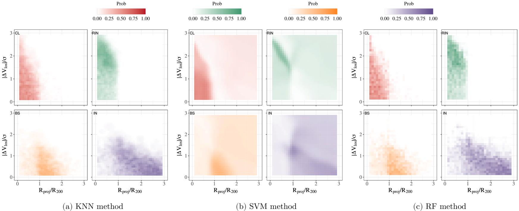
Figure 4: Mean class-probability in the PPSD for galaxies in the validation-set. Panel (a) shows the results obtained with the KNN method, panel (b) SVM method, and panel (c) RF method. In each case, different sub-panels correspond to galaxies classified as CL (red), RIN (green), BS (orange), and IN (violet).

3.1.1 Classification from the class-probability and testing the ML methods

With the estimated class-probabilities, there are at least three straightforward schemes for classifying a galaxy:

(a) The class is given by the highest class-probability.

(b) The class is given by a random pick of the five classes taking into account the estimated class-probabilities. Briefly, given a galaxy with class probabilities, $p_{i}$, where $\sum_{i=1}^{5}p_{i}=1$, we choose the class using the R-function sample setting the parameter prob $=p_{i}$.

(c) The class is given by the class-probability that is higher than a certain threshold.

Another utility of the class-probabilities is their use in weighted statistics. There might be situations in which it is not desirable to split galaxies in the sample under study into classes, but to use all galaxies in statistics which involve a weighting scheme. The estimated class-probabilities can be used as such weights.

In order to compare the performance of the ML methods, we define the following statistics:

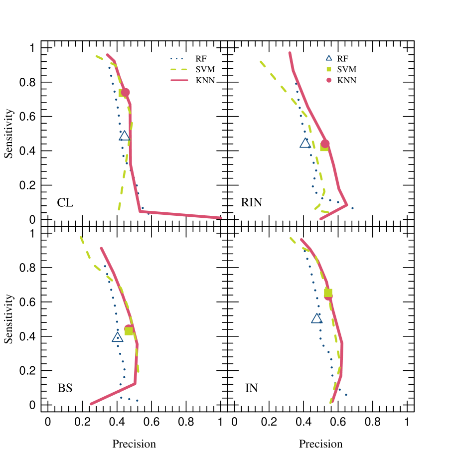
Figure 5: Sensitivity vs. precision of the trained ML algorithms represented by different curves. Results are obtained using the scheme (c) that considers a probability threshold as a parameter. In the curves shown, the parameter ranges from 0.1 at the upper end to 0.9 at the lower end. We show as blue triangle, light-green square and red filled circle the sensitivity and precision obtained when classifying galaxies taking into account the class with the highest probability. Each panel corresponds to a different class of galaxy in the training-set: cluster galaxies (upper left panel), recent infallers (upper right panel) backsplash galaxies, (lower left panel), and infalling galaxies (lower right panel).

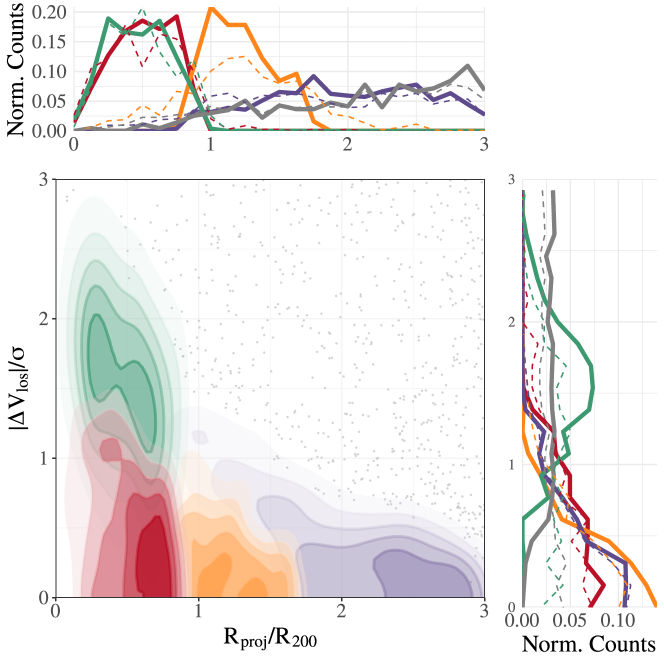
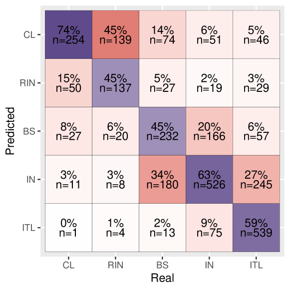
(a) KNN method

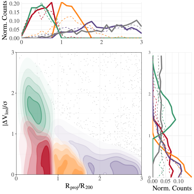
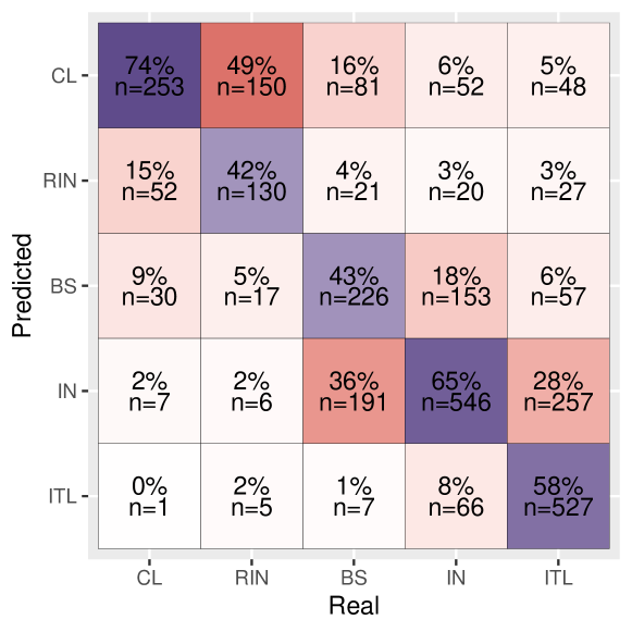
(b) SVM method

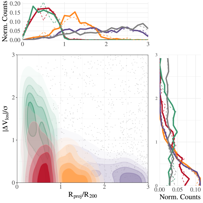
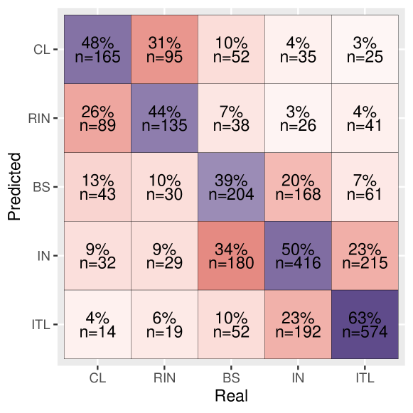
(c) RF method

Figure 6: Left panels: Phase-space ROGER classification of the galaxies in the validation-set determined by the highest class-probability using the three different ML techniques: KNN method (panel a), SVM method (panel b), and RF method (panel c). Symbols and colours are as in Fig. 3. Marginalised normalised distributions are shown at the top and at the right side of each panel in continuous lines. We have included as dashed lines the ‘true’ distributions shown in the right panel of Fig. 3. Right panels: Confusion matrices associated with the classification of the left panels.

• Sensitivity: the number of correct predictions of a given class in the resulting sample, divided by the total number of galaxies of that class in the validation-set.

• Precision: the number of correctly predicted galaxies of a given class in the resulting sample, divided by the total number of galaxies of that class in the resulting sample.

Using the scheme (c) above, and taking the probability threshold as a parameter, we can construct different resulting samples. This procedure, in turn, allows us to build a curve in the sensitivity-precision space. In Fig. 5, we show sensitivity vs. precision, for each of the trained algorithms, parameterised by the threshold value, that varies from $0.1$ (corresponding to the extreme of each curve in the upper left corner of each panel) to $0.9$ (the other extreme of the curves). It is important to remark that, given a certain threshold, there can be galaxies in the validation-set with all their probabilities lower than this value, and so, they will not be classified, and consequently, the sensitivity of the method will be reduced. In some extreme cases (see for example the SVM classification for backsplash galaxies) the are no galaxies with a probability higher than a threshold of 0.6, making it impossible to compute the sensitivity and precision. We also show in this figure as a blue triangle, light-green square and red filled circle the sensitivity vs. precision achieved for each method when classifying galaxies taking into account the class with the highest probability (scheme (a) above).

As expected, the sensitivity decreases as the probability threshold increases. This happens because increasing the threshold reduces the number of galaxies of each class in the resulting sample, thus the sensitivity is also reduced. It is also expected that the precision increases with increasing probability threshold. It can be seen that in general this is the case, with some few exceptions. This can be understood in terms of the overlapping of the different classes in the phase-space diagram. Thus there are regions in which, although the machine learning methods may compute a high probability for a galaxy of being of a certain class, there could also be many galaxies of other classes. In these regions, an important degree of contamination is expected.

As an example of the ML predictions, we show in the left panels of Fig. 6 the PPSD of the validation-set, where the classification of the galaxies is determined by the highest class-probability. Additionally, we show in solid lines the corresponding $R_{\rm proj}/R_{200}$ and $|\Delta V_{\rm los}|/\sigma$ marginalised distribution for the estimated classification, while in dashed lines we show the ‘true’ distributions corresponding to the validation-set (same as right panel of Fig. 3). It can be seen that, although the algorithm is capable of recovering similar trends as in Fig. 3, there are regions in which the different classes overlap and so, this echoes in contamination on the resulting samples. As discussed above, an important feature in Fig. 3 is that some classes overlap more with the rest than others. For instance, it is more likely for miss-classified cluster galaxies to be classified as recent infallers than as backsplash or infallers. This implies that in the resulting predictions the miss-classification will not be at random.

A useful way to visualise the performance of an algorithm is through the confusion matrix. Each row of this matrix represents the instances of each predicted class, while each column represents the instances of each real class. On the one hand, from the diagonal of this matrix we can read the sensitivity of the method when classifying the different types of galaxies. On the other hand, from the off-diagonal terms we can see the miss-classifications. In the right panels of Fig. 6, we present the confusion matrices of the classification shown in the left panels, quoting the percentages of galaxies of each real class that were classified as belonging to each predicted class. For instance, when using the KNN method, out of the real CL galaxies, 74 per cent are well classified. The remaining 26 per cent were classified as RIN (15 per cent), as BS (8 per cent), as IN (3 per cent) and as INT (0 per cent). The row corresponding to CL galaxies shows that 45 per cent of the real RIN galaxies, 14 per cent of the real BS galaxies, the 6 per cent of the real IN galaxies, and the 5 per cent of the real ITL galaxies were classified as CL. We find that the KNN method achieves a sensitivity of 74 per cent, 45 per cent, 45 per cent, 63 per cent, and 59 per cent when classifying galaxies as CL, RIN, BS, IN, and ITL, respectively. The SVM method achieves a 74 per cent, 42 per cent, 43 per cent, 65 per cent, and 58 per cent of sensitivity, while the RF method achieves 48 per cent, 44 per cent, 39 per cent, 50 per cent, and 63 per cent of sensitivity. It should be kept in mind that these numbers correspond to the classification taking into account the highest class-probability (scheme (a)), and they will change if the classification is performed with another scheme. Another feature worth remarking is that, although the RF method recovers distributions more similar to the real ones, its performance is poorer than the SVM and KNN methods in terms of both sensitivity and precision.

Finally, as the ROGER software gives as output the class-probability of a galaxy of belonging to each class, we can build a random realisation of a particular cluster, by randomly classifying each galaxy as explained in scheme (b). An example of such procedure is given in Sec. 3.1.2.

Taking into account the results shown in this section, the method of our preference is KNN. It has two main advantages: it is the simplest one, and performs similarly or better than the more complex SVM and RF methods. We remark that in the ROGER package the three methods are available.

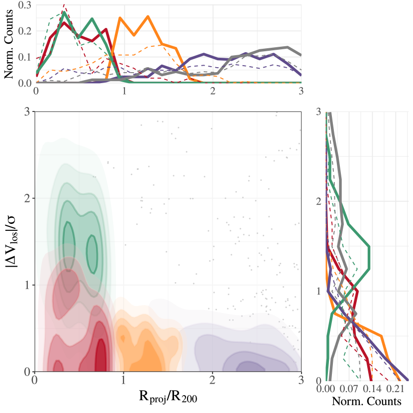
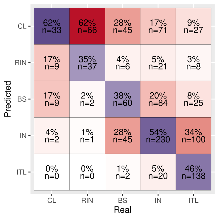
Figure 7: Left panel: Phase-space ROGER classification of the galaxies in the test cluster using the KNN method and the highest class-probability for each galaxy. We show in different colour shades the density of galaxies classified as CL (red), RIN (green), BS (orange), and IN (violet). ITL galaxies are shown as individual gray points for clarity. In the upper and right sub-panels, we show the marginalised distributions of projected distance and line-of-sight velocity of galaxies, respectively, according to the ROGER classification (continuous lines) and the ’real’ classification (dashed lines). Right panel: confusion matrix associated to the left panel.

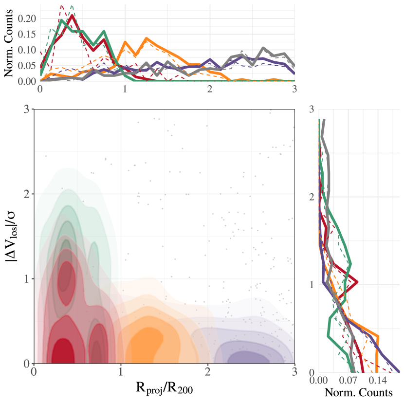
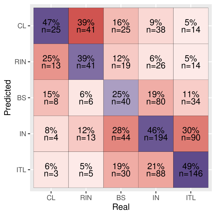
Figure 8: Left panel: Phase-space ROGER classification of the galaxies in the test cluster using the KNN method and a random realisation considering the class-probabilities for each galaxy. We show in different colour shades the density of galaxies classified as CL (red), RIN (green), BS (orange), and IN (violet). ITL galaxies are shown as individual gray points for clarity. In the upper and right sub-panels, we show the marginalised distributions of projected distance and line-of-sight velocity of galaxies, respectively, according to the ROGER classification (continuous lines) and the ‘real’ classification (dashed lines). Right panel: confusion matrix associated to the left panel.

3.1.2 Testing the methods in an independent cluster

As a further test, and to provide an end-to-end example, we analyse the cluster that was previously left aside from both the training and validation sets. Several jupyter notebooks with full examples are provided on the github repository. We also include an appendix (A) where we show the basic options included in the ROGER software.

In the left panel of Fig. 7, we show the PPSD of the test galaxy cluster, where different colours refer to the types of galaxies as predicted by the KNN method by taking into account the highest class-probability. We show the resulting confusion matrix in the right panel of Fig. 7.

Finally, we create a random realisation of the test cluster following the scheme (b) as explained in the previous subsection. In the left panel of Fig. 8, we show the PPSD of the random realisation for the test cluster and its surroundings. The corresponding marginalised distributions are represented by solid lines. For a better comparison, in dashed lines, we add the marginalised distributions of galaxy projected distance and line-of-sight velocity taking into account their real classes. As it can be seen from this figure, the distributions in both axis of the random realisation agree well with the real distributions of the galaxies, which demonstrate the ability of the method to learn the real properties of each galaxy class. In the right panel of Fig. 8, we show the corresponding confusion matrix. The classification obtained by taking into account the highest class-probability achieves a better performance in terms of the confusion matrix, nevertheless the random realisation reproduces better the overall distributions.

The results of applying the ROGER algorithm to a sample of galaxies completely independent of the samples used for training and validation follow the same trends and are consistent with the results obtained during the validation process (see Figs. 5 and 6).

4 Conclusions

We have developed ROGER, a machine learning technique-based algorithm that classifies galaxies by relating their position in the projected phase space diagram with their three-dimensional orbits. This algorithm was trained using a galaxy catalogue generated from the MDPL2 cosmological simulation and the SAG semi-analytic model of galaxy formation. The volume of this simulation is large enough to have a statistically significant sample of massive isolated clusters and galaxies, which we used to study different machine learning methods. For each galaxy, these methods give as output the probability of being a cluster galaxy, a recent infaller, a backsplash galaxy, an infalling galaxy or an interloper galaxy. Classifying galaxies into these five classes is useful in studies in which it is necessary to know the past trajectory of galaxies, in order to understand how different physical mechanisms have acted upon them. As an example, let us consider a backsplash and a recent infaller, they may both be satellites of a cluster, however, their past histories are different. The former has been all the way into the cluster and out, while the latter has just dived into the cluster. We should expect them to have different physical properties.

Considering a classification scheme that adopts different probability thresholds, we were able to build different final samples with different contamination and sensitivity. We found that the method with the best performance is the K-Nearest Neighbours method, achieving a 74 per cent, 45 per cent, 45 per cent, 63 per cent and 59 per cent of sensitivity when classifying cluster galaxies, recent infaller galaxies, backsplash galaxies, infaller galaxies and interloper galaxies, respectively (see Fig. 6). Although the other methods have similar performances and are available in the ROGER software, we choose the KNN method as our preferred algorithm for its simplicity.

Finally, with the aim of providing a fully consistent and automatic algorithm for the classification of galaxies in the PPSD, we present ROGER, an R-package that is publicly available through the github repository: https://github.com/Martindelosrios/ROGER/.

Data availability

The data underlying this article are available in https://github.com/Martindelosrios/ROGER at https://zenodo.org/badge/latestdoi/224241400

Appendix A ROGER examples

This is a simple example of the basic use of the ROGER software in an R-console.

Once the library is installed, we begin by loading the ROGER library

library(‘ROGER’)

Assuming that the data of a galaxy cluster is loaded in a data-frame called ‘cat’ with the projected phase-space information of each galaxy, that have at least two columns named ‘r’ (projected radius in units of $R_{200}$), and ‘v’ (line-of-sight velocity relative to the cluster in units of the cluster velocity dispersion $\sigma$), we can just run the following script to estimate the class-probability of each galaxy using the trained KNN algorithm.

pred_prob <- get_class(cat, model = knn,
             type = ‘prob’)

This will give as an output a data-frame with five columns that correspond to the five class-probabilities. It is worth to remark that the user can use the SVM or the RF method just changing the model option with ‘svm’ or ‘rf’, respectively. The user can also change the type of prediction from ‘prob’ to ‘class’ in order to directly predict the most probable class, or set a probability threshold value putting ‘threshold $=x$’ to classify galaxies that have the corresponding class-probability higher that the selected value.

References

- Abadi et al. (1999) Abadi M. G., Moore B., Bower R. G., 1999, MNRAS, 308, 947
- Aguerri & Sánchez-Janssen (2010) Aguerri J. A. L., Sánchez-Janssen R., 2010, A&A, 521, A28
- Bahé et al. (2013) Bahé Y. M., McCarthy I. G., Balogh M. L., Font A. S., 2013, MNRAS, 430, 3017
- Balogh et al. (1999) Balogh M. L., Morris S. L., Yee H. K. C., Carlberg R. G., Ellingson E., 1999, ApJ, 527, 54
- Balogh et al. (2000) Balogh M. L., Navarro J. F., Morris S. L., 2000, ApJ, 540, 113
- Beers et al. (1990) Beers T. C., Flynn K., Gebhardt K., 1990, AJ, 100, 32
- Behroozi et al. (2013a) Behroozi P. S., Wechsler R. H., Wu H.-Y., 2013a, ApJ, 762, 109
- Behroozi et al. (2013b) Behroozi P. S., Wechsler R. H., Wu H.-Y., Busha M. T., Klypin A. A., Primack J. R., 2013b, ApJ, 763, 18
- Bekki (2009) Bekki K., 2009, MNRAS, 399, 2221
- Bom et al. (2017) Bom C. R., Makler M., Albuquerque M. P., Brandt C. H., 2017, A&A, 597, A135
- Book & Benson (2010) Book L. G., Benson A. J., 2010, ApJ, 716, 810
- Breiman (2001) Breiman L., 2001, Machine Learning, 45, 5
- Byrd & Valtonen (2001) Byrd G., Valtonen M., 2001, AJ, 121, 2943
- Collacchioni et al. (2018) Collacchioni F., Cora S. A., Lagos C. D. P., Vega-Martínez C. A., 2018, MNRAS, 481, 954
- Cora (2006) Cora S. A., 2006, MNRAS, 368, 1540
- Cora et al. (2018) Cora S. A., et al., 2018, MNRAS, 479, 2
- Cora et al. (2019) Cora S. A., Hough T., Vega-Martínez C. A., Orsi Á. A., 2019, MNRAS, 483, 1686
- Cortes & Vapnik (1995) Cortes C., Vapnik V., 1995, Machine Learning, 20, 273
- de los Rios et al. (2016) de los Rios M., Domínguez R. M. J., Paz D., Merchán M., 2016, MNRAS, 458, 226
- De Lucia et al. (2012) De Lucia G., Weinmann S., Poggianti B. M., Aragón-Salamanca A., Zaritsky D., 2012, MNRAS, 423, 1277
- Diaz Rivero & Dvorkin (2020) Diaz Rivero A., Dvorkin C., 2020, Physical Review D, 101
- Fujita (2004) Fujita Y., 2004, PASJ, 56, 29
- Gao et al. (2004) Gao L., White S. D. M., Jenkins A., Stoehr F., Springel V., 2004, MNRAS, 355, 819
- Gargiulo et al. (2015) Gargiulo I. D., et al., 2015, MNRAS, 446, 3820
- Gill et al. (2005) Gill S. P. D., Knebe A., Gibson B. K., 2005, MNRAS, 356, 1327
- Gnedin (2003a) Gnedin O. Y., 2003a, ApJ, 582, 141
- Gnedin (2003b) Gnedin O. Y., 2003b, ApJ, 589, 752
- Gunn & Gott (1972) Gunn J. E., Gott J. R. I., 1972, ApJ, 176, 1
- Hernández-Fernández et al. (2014) Hernández-Fernández J. D., Haines C. P., Diaferio A., Iglesias-Páramo J., Mendes de Oliveira C., Vilchez J. M., 2014, MNRAS, 438, 2186
- Hess & Wilcots (2013) Hess K. M., Wilcots E. M., 2013, AJ, 146, 124
- Hou et al. (2014) Hou A., Parker L. C., Harris W. E., 2014, MNRAS, 442, 406
- Jaffé et al. (2012) Jaffé Y. L., Poggianti B. M., Verheijen M. A. W., Deshev B. Z., van Gorkom J. H., 2012, ApJL, 756, L28
- Jaffé et al. (2015) Jaffé Y. L., Smith R., Candlish G. N., Poggianti B. M., Sheen Y.-K., Verheijen M. A. W., 2015, MNRAS, 448, 1715
- Jaffé et al. (2018) Jaffé Y. L., et al., 2018, MNRAS, 476, 4753
- Kawata & Mulchaey (2008) Kawata D., Mulchaey J. S., 2008, ApJL, 672, L103
- Klypin et al. (2016) Klypin A., Yepes G., Gottlöber S., Prada F., Heß S., 2016, MNRAS, 457, 4340
- Knebe et al. (2018) Knebe A., et al., 2018, MNRAS, 474, 5206
- Kuhn (2020) Kuhn M., 2020, caret: Classification and Regression Training. https://CRAN.R-project.org/package=caret
- Lagos et al. (2008) Lagos C. d. P., Cora S. A., Padilla N. D., 2008, MNRAS, 388, 587
- Larson et al. (1980) Larson R. B., Tinsley B. M., Caldwell C. N., 1980, ApJ, 237, 692
- Limousin et al. (2009) Limousin M., Sommer-Larsen J., Natarajan P., Milvang-Jensen B., 2009, ApJ, 696, 1771
- Łokas et al. (2016) Łokas E. L., Ebrová I., del Pino A., Sybilska A., Athanassoula E., Semczuk M., Gajda G., Fouquet S., 2016, ApJ, 826, 227
- Mahajan et al. (2011) Mahajan S., Mamon G. A., Raychaudhury S., 2011, MNRAS, 416, 2882
- McCarthy et al. (2008) McCarthy I. G., Frenk C. S., Font A. S., Lacey C. G., Bower R. G., Mitchell N. L., Balogh M. L., Theuns T., 2008, MNRAS, 383, 593
- McGee et al. (2009) McGee S. L., Balogh M. L., Bower R. G., Font A. S., McCarthy I. G., 2009, MNRAS, 400, 937
- Mihos (2004) Mihos J. C., 2004, Cambridge: Cambridge Univ. Press, ed. J. S. Mulchaey, A. Dressler, & A. Oemler, p. 277
- Moore et al. (1996) Moore B., Katz N., Lake G., Dressler A., Oemler A., 1996, Nature, 379, 613
- Moore et al. (1998) Moore B., Lake G., Katz N., 1998, ApJ, 495, 139
- Muñoz Arancibia et al. (2015) Muñoz Arancibia A. M., Navarrete F. P., Padilla N. D., Cora S. A., Gawiser E., Kurczynski P., Ruiz A. N., 2015, MNRAS, 446, 2291
- Munari et al. (2013) Munari E., Biviano A., Borgani S., Murante G., Fabjan D., 2013, MNRAS, 430, 2638
- Muriel & Coenda (2014) Muriel H., Coenda V., 2014, A&A, 564, A85
- Muzzin et al. (2014) Muzzin A., et al., 2014, ApJ, 796, 65
- Oman & Hudson (2016) Oman K. A., Hudson M. J., 2016, MNRAS, 463, 3083
- Oman et al. (2013) Oman K. A., Hudson M. J., Behroozi P. S., 2013, MNRAS, 431, 2307
- Pasquali et al. (2019) Pasquali A., Smith R., Gallazzi A., De Lucia G., Zibetti S., Hirschmann M., Yi S. K., 2019, MNRAS, 484, 1702
- Planck Collaboration et al. (2014) Planck Collaboration et al., 2014, A&A, 571, A16
- Planck Collaboration et al. (2016) Planck Collaboration et al., 2016, A&A, 594, A13
- Rasmussen et al. (2006) Rasmussen J., Ponman T. J., Mulchaey J. S., 2006, MNRAS, 370, 453
- Rhee et al. (2017) Rhee J., Smith R., Choi H., Yi S. K., Jaffé Y., Candlish G., Sánchez-Jánssen R., 2017, ApJ, 843, 128
- Riebe et al. (2013) Riebe K., et al., 2013, Astronomische Nachrichten, 334, 691
- Rines & Diaferio (2005) Rines K., Diaferio A., 2005, in American Astronomical Society Meeting Abstracts. p. 101.03
- Ruiz et al. (2015) Ruiz A. N., et al., 2015, ApJ, 801, 139
- Semczuk et al. (2017) Semczuk M., Łokas E. L., del Pino A., 2017, ApJ, 834, 7
- Smith et al. (2015) Smith R., et al., 2015, MNRAS, 454, 2502
- Smith et al. (2019) Smith R., Pacifici C., Pasquali A., Calderón-Castillo P., 2019, ApJ, 876, 145
- Steinhauser et al. (2016) Steinhauser D., Schindler S., Springel V., 2016, A&A, 591, A51
- Tecce et al. (2010) Tecce T. E., Cora S. A., Tissera P. B., Abadi M. G., Lagos C. d. P., 2010, MNRAS, 408, 2008
- Vijayaraghavan & Ricker (2015) Vijayaraghavan R., Ricker P. M., 2015, MNRAS, 449, 2312
- Villalobos et al. (2014) Villalobos Á., De Lucia G., Murante G., 2014, MNRAS, 444, 313
- Wetzel et al. (2013) Wetzel A. R., Tinker J. L., Conroy C., van den Bosch F. C., 2013, MNRAS, 432, 336
- Yoon et al. (2017) Yoon H., Chung A., Smith R., Jaffé Y. L., 2017, ApJ, 838, 81
- Zwicky (1951) Zwicky F., 1951, PASP, 63, 17