The subtraction contribution to the muonic-hydrogen Lamb shift: a point for lattice QCD calculations of the polarizability effect

Abstract

The proton-polarizability contribution to the muonic-hydrogen Lamb shift is a major source of theoretical uncertainty in the extraction of the proton charge radius. An empirical evaluation of this effect, based on the proton structure functions, requires a systematically improvable calculation of the “subtraction function”, possibly using lattice QCD. We consider a different subtraction point, with the aim of accessing the subtraction function directly in lattice calculations. A useful feature of this subtraction point is that the corresponding contribution of the structure functions to the Lamb shift is suppressed. The whole effect is dominated by the subtraction contribution, calculable on the lattice.

I Introduction — The point of subtraction

The nucleon structure functions are used as input in calculations of the nuclear structure effects in precision atomic spectroscopy (see Pohl et al. (2013); Carlson (2015); Hagelstein et al. (2016); Pasquini and Vanderhaeghen (2018) for reviews). The muonic-hydrogen ($\mu$H) experiments demand a higher quality of this input in both the Lamb shift Pohl et al. (2010); Antognini et al. (2013) and hyperfine structure Pohl et al. (2016); Bakalov et al. (2015); Kanda et al. (2018). In the Lamb-shift calculations, however, the problem is severed by the fact that, in addition to the unpolarized structure functions $F_{1}(x,Q^{2})$ and $F_{2}(x,Q^{2})$, one encounters a “subtraction function” which is largely unknown. Thus, the subtraction-function contribution to the Lamb shift precludes insofar any systematic improvement of the theoretical uncertainty of the “data-driven” evaluations, based on dispersion relations alone.

Ultimately, one should aim at calculating the subtraction-function contribution in lattice QCD (LQCD). Some efforts in this direction have already been made Ji and Jung (2001); Chambers et al. (2017); Can et al. (2020); Hannaford-Gunn et al. (2020) In the present work we propose an unconventional choice of the subtraction point, which, first of all, is directly accessible in lattice calculations, and secondly, diminishes the structure-function contribution.

Figure 1: Forward doubly-virtual Compton scattering process.

We start by considering the forward doubly-virtual Compton scattering (VVCS) amplitude (cf. Fig. 1):

$$T^{\mu\nu}(p,q)=i\int d^{4}x\,e^{-iq\cdot x}\,\big{\langle}N(p)\big{|}T\big{(}j^{\mu}(x)\,j^{\nu}(0)\big{)}\big{|}N(p)\big{\rangle},$$ (1)

with $p$ and $q$ the target and photon four-momenta, respectively. For an unpolarized target (of any spin), the forward VVCS amplitude decomposes into two Lorentz structures:

$$T^{\mu\nu}(p,q)=\left(-g^{\mu\nu}+\frac{q^{\mu}q^{\nu}}{q^{2}}\right)T_{1}(\nu,Q^{2})+\frac{1}{M^{2}}\left(p^{\mu}-\frac{p\cdot q}{q^{2}}\,q^{\mu}\right)\left(p^{\nu}-\frac{p\cdot q}{q^{2}}\,q^{\nu}\right)T_{2}(\nu,Q^{2}),$$ (2)

where $\sqrt{p^{2}}=M$ is the target mass. The two scalar amplitudes $T_{1,2}$ are functions of the photon energy $\nu=p\cdot q/M$ and the virtuality $Q^{2}=-q^{2}$.

Figure 2: Forward two-photon exchange in a hydrogen-like atom.

The two-photon exchange (TPE) correction to the $n$-th $S$-level of a hydrogen-like atom, shown in Fig. 2, is subleading to the well-known proton charge radius effect. To order $\alpha^{5}$, the TPE contribution is expressed entirely in terms of the forward VVCS amplitudes:

$$\Delta E_{nS}=8\pi\alpha m\,\phi_{n}^{2}\,\frac{1}{i}\int_{-\infty}^{\infty}\!\frac{\mathrm{d}\nu}{2\pi}\int\!\!\frac{\mathrm{d}\mathbf{q}}{(2\pi)^{3}}\frac{\left(Q^{2}-2\nu^{2}\right)T_{1}(\nu,Q^{2})-(Q^{2}+\nu^{2})\,T_{2}(\nu,Q^{2})}{Q^{4}(Q^{4}-4m^{2}\nu^{2})},$$ (3)

where $\alpha$ is the fine-structure constant, $\phi_{n}^{2}=1/(\pi n^{3}a^{3})$ is the Coulomb wave-function at the origin, $a=(Z\alpha m_{r})^{-1}$ is the Bohr radius, $m_{r}=mM/(m+M)$ is the reduced mass, $M$ and $m$ are the nucleus and lepton masses, and $Z$ is the charge of the nucleus (in the following we assume $Z=1$).

To date, all the data-driven evaluations of the TPE effect in $\mu$H, employ the following dispersion relations:

$$T_{1}(\nu,Q^{2}) = T_{1}(0,Q^{2})+\frac{32\pi\alpha M\nu^{2}}{Q^{4}}\int_{0}^{1}\,\mathrm{d}x\,\frac{x\,F_{1}(x,Q^{2})}{1-x^{2}(\nu/\nu_{\mathrm{el}})^{2}-i0^{+}},$$ (4a)

$$T_{2}(\nu,Q^{2}) = \frac{16\pi\alpha M}{Q^{2}}\int_{0}^{1}\!\mathrm{d}x\,\frac{F_{2}(x,Q^{2})}{1-x^{2}(\nu/\nu_{\mathrm{el}})^{2}-i0^{+}},$$ (4b)

with $\nu_{\mathrm{el}}=\nicefrac{{Q^{2}}}{{2M}}$ and the Bjorken variable $x$. Note that, while $T_{2}$ is fully determined by the empirical proton structure function $F_{2}(x,Q^{2})$, the amplitude $T_{1}$ is determined by $F_{1}(x,Q^{2})$ only up to the subtraction function at $\nu=0$. This is because the high-energy behaviour of the proton structure function $F_{1}$ requires at least one subtraction for a valid dispersion relation.

The point of subtraction, however, is rather arbitrary. Recently, Gasser, Leutwyler and Rusetsky have considered the subtraction at $\nu=\mbox{$\frac{1}{2}$}iQ$ and argued that it is advantageous in the context of the Cottingham formula for the proton-neutron mass splitting Gasser et al. (2020). Here, we find that the subtraction at $\nu=iQ$ leads to interesting ramifications for the $\mu$H Lamb-shift evaluation. In this case, for example, the so-called “inelastic contribution” (i.e., the contributions of inelastic structure functions $F_{1}$ and $F_{2}$) becomes negligible. In what follows, we go through the main steps of the formulae, present numerical results based on the Bosted-Christy parametrization of proton structure functions Christy and Bosted (2010), and discuss the prospects for future lattice calculations of these effects.

II Standard formulae

Recall that the VVCS amplitudes can be split unambiguously into Born and polarizability pieces:

$$T_{i}=T_{i}^{\mathrm{Born}}+\overline{T}_{i},$$ (5)

with the Born term given entirely by the elastic form factors $G_{E}(Q^{2})$ and $G_{M}(Q^{2})$, whereas the remainder $\overline{T}_{i}$ is, in the low-energy limit, characterised by polarizabilities, e.g.:

$$\overline{T}_{1}(\nu,Q^{2}) = 4\pi\left[\beta_{M1}Q^{2}+\big{(}\alpha_{E1}+\beta_{M1}\big{)}\nu^{2}\right]+O(Q^{4},\nu^{4},Q^{2}\nu^{2})$$ (6a)

$$\overline{T}_{2}(\nu,Q^{2}) = 4\pi\big{(}\alpha_{E1}+\beta_{M1}\big{)}Q^{2}+O(Q^{4},\nu^{4},Q^{2}\nu^{2}),$$ (6b)

where $\alpha_{E1}$ ($\beta_{M1}$) is the electric (magnetic) dipole polarizability. In general, the polarizability term by itself satisfies the aforementioned dispersion relations (omitting the $i0^{+}$ prescription from now on) :

$$\overline{T}_{1}(\nu,Q^{2}) = \overline{T}_{1}(0,Q^{2})+\frac{32\pi\alpha M\nu^{2}}{Q^{4}}\int_{0}^{x_{0}}\,\mathrm{d}x\,\frac{x\,F_{1}(x,Q^{2})}{1-x^{2}(\nu/\nu_{\mathrm{el}})^{2}},$$ (7a)

$$\overline{T}_{2}(\nu,Q^{2}) = \frac{16\pi\alpha M}{Q^{2}}\int_{0}^{x_{0}}\!\mathrm{d}x\,\frac{F_{2}(x,Q^{2})}{1-x^{2}(\nu/\nu_{\mathrm{el}})^{2}}.$$ (7b)

The only distinction with the above Eq. (4) is the upper limit of integration over the Bjorken-$x$, which is now set by an inelastic threshold $x_{0}$, thus excluding explicitly the elastic contribution.

The full TPE calculation, in the data-driven approach based on dispersion relations, is then split into three contribution: elastic, inelastic and subtraction. The elastic one follows directly from the Born contribution to VVCS amplitudes and it yields essentially the effect of the Friar radius (a.k.a., the 3^rd Zemach moment). The other two contributions follow from the polarizability piece, such that the inelastic contribution is given by the inelastic structure functions, whereas subtraction is the rest, i.e., the $nS$ level is affected as:

$$\Delta E^{(\mathrm{inel.})}_{nS} = -32\alpha^{2}Mm\,\phi_{n}^{2}\,\int_{0}^{\infty}\frac{\mathrm{d}Q}{Q^{5}}\,\int_{0}^{x_{0}}\frac{\mathrm{d}x}{(1+v_{l})(1+v_{x})}\Bigg{\{}\left[1+\frac{v_{l}v_{x}}{v_{l}+v_{x}}\right]F_{2}(x,Q^{2})$$ (8a)

$$+\frac{2x}{(1+v_{l})(1+v_{x})}\left[2+\frac{3+v_{l}v_{x}}{v_{l}+v_{x}}\right]F_{1}(x,Q^{2})\Bigg{\}},$$

$$\Delta E^{\mathrm{(subtr.)}}_{nS} = \frac{2\alpha m}{\pi}\,\phi_{n}^{2}\,\int_{0}^{\infty}\frac{\mathrm{d}Q}{Q^{3}}\frac{2+v_{l}}{(1+v_{l})^{2}}\,\overline{T}_{1}(0,Q^{2}),$$ (8b)

with the following definitions:

$$v_{x} = \sqrt{1+x^{2}\tau^{-1}},\qquad\tau=\frac{Q^{2}}{4M^{2}},$$ (9a)

$$v_{l} = \sqrt{1+\tau_{l}^{-1}},\qquad\tau_{l}=\frac{Q^{2}}{4m^{2}}.$$ (9b)

These are the standard formulae, where the subtraction is made at $\nu=0$.

III A different subtraction point

Now, for the subtraction at $\nu=iQ$, the subtracted dispersion relation reads as:

$$\overline{T}_{1}(\nu,Q^{2})=\overline{T}_{1}(iQ,Q^{2})+\frac{32\pi\alpha M}{Q^{4}}\left(\nu^{2}+Q^{2}\right)\int_{0}^{x_{0}}\mathrm{d}x\,x\,\frac{F_{1}(x,Q^{2})}{\big{[}1-x^{2}(\nu/\nu_{\mathrm{el}})^{2}\big{]}\big{(}1+x^{2}\tau^{-1}\big{)}}.$$ (10)

Hence, the inelastic and subtraction contributions change into:

$$\Delta E^{\prime\,(\mathrm{inel.})}_{nS} = -32\alpha^{2}Mm\phi_{n}^{2}\int_{0}^{\infty}\frac{\mathrm{d}Q}{Q^{5}}\int_{0}^{x_{0}}\ \mathrm{d}x\,\Bigg{\{}\frac{1}{(1+v_{l})(1+v_{x})}\left[1+\frac{v_{l}v_{x}}{v_{l}+v_{x}}\right]F_{2}(x,Q^{2})$$ (11a)

$$+\frac{x}{2}\frac{1}{v_{x}^{2}(v_{l}^{2}-v_{x}^{2})}\left[x^{2}\frac{3+9v_{x}+4v_{x}^{2}}{\tau\,(1+v_{x})^{3}}-\frac{3+9v_{l}+4v_{l}^{2}}{\tau_{l}\,(1+v_{l})^{3}}\right]\,F_{1}(x,Q^{2})\Bigg{\}},$$

$$\Delta E^{\prime\,\mathrm{(subtr.)}}_{nS} = \frac{2\alpha m}{\pi}\phi_{n}^{2}\int_{0}^{\infty}\frac{\mathrm{d}Q}{Q^{3}}\frac{2+v_{l}}{(1+v_{l})^{2}}\,\overline{T}_{1}(iQ,Q^{2}).$$ (11b)

Of course the sum of the two, i.e., the polarizability contribution, remains to be the same,

$$\Delta E^{\text{(pol.)}}_{nS}=\Delta E^{\text{(inel.)}}_{nS}+\Delta E^{\text{(subtr.)}}_{nS}=\Delta E^{\prime\,(\mathrm{inel.})}_{nS}+\Delta E^{\prime\,\mathrm{(subtr.)}}_{nS}.$$ (12)

What changes is the relative size of the two contributions: while for the subtraction at zero the inelastic contribution is relatively large, for the subtraction at $iQ$ it is negligible at the current level of experimental precision ($\sim 2\,\upmu$eV). For example, substituting the commonly used Bosted-Christy parametrization of the structure functions (limited to the region $0\leq Q^{2}\leq 8$ GeV² and $1.1\leq W\leq 3.1$ GeV) Christy and Bosted (2010), we obtain:

$$\Delta E^{(\mathrm{inel.})}_{2S}\simeq-12.3\,\upmu\text{eV},\quad\mbox{versus}\quad\Delta E^{\prime\,(\mathrm{inel.})}_{2S}\simeq 1.6\,\upmu\text{eV}.$$ (13)

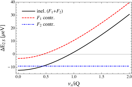
Figure 3: Inelastic contribution to the $\mu$H Lamb shift as function of an arbitrary subtraction point $\nu_{s}$.

For an arbitrary subtraction point $\nu_{s}$, the situation is illustrated in Fig. 3, where the inelastic contribution, along with the separate contributions of $F_{1}$ and $F_{2}$ is considered as function of $\nu_{s}/iQ$. The values shown in Eq. (13) correspond with the black curve at 0 and 1 respectively. One can see that the inelastic contribution vanishes in the vicinity of $\nu_{s}=iQ$. This happens for a combination of reasons, but to give a simple explanation consider the following.

The TPE effect in the Lamb shift is dominated by longitudinal photons, and as a result by the electric form factor and the electric polarizability. The conventional subtraction function is, however, dominated by transverse photons and the magnetic polarizability, $\overline{T}_{1}(0,Q^{2})=4\pi\beta_{M1}Q^{2}+O(Q^{4})$. The dominant effect is therefore contained in the inelastic contribution. For the subtraction at $iQ$, the subtraction function is equivalent to the purely longitudinal amplitude, defined as $T_{L}=-T_{1}+(1+\nu^{2}/Q^{2})T_{2}$, which at low $Q^{2}$ is given by the electric polarizability:

$$\overline{T}_{L}(iQ,Q^{2})=-\overline{T}_{1}(iQ,Q^{2})=4\pi\alpha_{E1}Q^{2}+O(Q^{4}).$$ (14)

At the same time, the integrand of the inelastic contribution is, at low $Q$, given by the longitudinal function, $F_{L}=-2xF_{1}+F_{2}$. This particular combination of structure functions is suppressed at low $Q$, due to gauge invariance. As the result, the dominant contribution is contained solely in the subtraction function.

Concerning the transverse contributions, note that for the conventional subtraction at 0 they cancel between the subtraction and inelastic contributions (e.g., the magnetic polarizability effect), whereas for the subtraction at $iQ$ they are absent form the subtraction function and cancel between the structure functions within the inelastic contribution.

IV Prospects for lattice calculations

The subtraction point at $iQ$ brings a few advantages for a LQCD evaluation of the polarizability effect. First LQCD calculations of the nucleon VVCS Can et al. (2020); Hannaford-Gunn et al. (2020); Chambers et al. (2017), employing the Feynman-Hellmann theorem Ji and Jung (2001), isolate $T_{1}(\nu,Q^{2})$ in the unphysical region. They obtain results for $Q^{2}\in\{3\dots 7\}$ GeV² Can et al. (2020), with the main aim to compute the moments of $F_{1}$, which is done by extrapolating to $\nu=0$. The calculation of the Lamb-shift contribution at the point $\nu=iQ$, proposed here, simply means setting the three-momentum of external photon to zero, $\vec{q}=0$. This point can be accessed directly in lattice calculations.

The second advantage is that the evaluation at the $iQ$ point ensures that the subtraction function gives nearly the entire effect; the impact of the empirical structure function contribution is minimal. This said, it would be interesting to test the lattice calculations of this effect with structure functions. This can for instance be done by calculation the VVCS amplitude $T_{1}$ at two different subtraction points. The difference can then be expressed through an integral of the structure function $F_{1}$. For example, the difference between the subtraction functions at 0 and $iQ$ points is given by

$$\overline{T}_{1}(0,Q^{2})-\overline{T}_{1}(iQ,Q^{2})=\frac{8\pi\alpha}{M}\int_{0}^{x_{0}}\mathrm{d}x\,\frac{x}{\tau+x^{2}}F_{1}(x,Q^{2}).$$ (15)

V Conclusions

We have considered the possibility of an ab initio calculation of the proton-polarizability contribution to the Lamb shift of hydrogen-like atoms. In a data-driven approach, one relies on the dispersion relations that determine this contribution in terms of empirical structure functions of the proton, albeit not entirely. The subtraction function, needed for a well-defined dispersion relation involving the structure function $F_{1}$, is not determined experimentally and is modeled. Present state-of-art dispersive calculations model the subtraction function, whereas the structure-function contributions are calculated by a double integration (over x and $Q^{2}$) of the empirical parametrizations of $F_{1}$ and $F_{2}$. Each piece of this splitting is affected by a large Delta-resonance contribution which must cancel in the total. The empirical and modeled pieces do not have exactly the same Delta-resonance physics, which makes the cancellation difficult to achieve in practice.

Ideally, the subtraction function should be calculated from LQCD. However, the problem of Delta-resonance cancellation would remain, because of the different systematics of the lattice versus empirical evaluation. In addition, the strict zero-energy limit is not directly accessible in lattice calculations. Here we have addressed both of these problems by considering a different subtraction point: $\nu=iQ$.

Besides the easier access of $T_{1}(iQ,Q^{2})$ in Euclidean finite-volume calculations, this choice has the other advantage: the polarizability contribution is dominated by the subtraction contribution; the structure-function contribution becomes suppressed, avoiding the large cancellations between these two contributions. Thus, while the subtraction function is directly accessed on the lattice, the structure function contribution is dramatically reduced and hence can be calculated to better precision, relative to the full contribution.

References

- Pohl et al. (2013) R. Pohl, R. Gilman, G. A. Miller, and K. Pachucki, Ann. Rev. Nucl. Part. Sci. 63, 175 (2013), arXiv:1301.0905 [physics.atom-ph] .
- Carlson (2015) C. E. Carlson, Prog. Part. Nucl. Phys. 82, 59 (2015), arXiv:1502.05314 [hep-ph] .
- Hagelstein et al. (2016) F. Hagelstein, R. Miskimen, and V. Pascalutsa, Prog. Part. Nucl. Phys. 88, 29 (2016), arXiv:1512.03765 [nucl-th] .
- Pasquini and Vanderhaeghen (2018) B. Pasquini and M. Vanderhaeghen, Ann. Rev. Nucl. Part. Sci. 68, 75 (2018), arXiv:1805.10482 [hep-ph] .
- Pohl et al. (2010) R. Pohl et al., Nature 466, 213 (2010).
- Antognini et al. (2013) A. Antognini, F. Nez, K. Schuhmann, F. D. Amaro, et al., Science 339, 417 (2013).
- Pohl et al. (2016) R. Pohl et al., in Proceedings, 12th International Conference on Low Energy Antiproton Physics (LEAP2016), Kanazawa, Japan, March 6-11, 2016 (2016) arXiv:1609.03440 [physics.atom-ph] .
- Bakalov et al. (2015) D. Bakalov, A. Adamczak, M. Stoilov, and A. Vacchi, Proceedings, 5th International Conference on Exotic Atoms and Related Topics (EXA2014): Vienna, Austria, September 15-19, 2014, Hyperfine Interact. 233, 97 (2015).
- Kanda et al. (2018) S. Kanda et al., J. Phys. Conf. Ser. 1138, 012009 (2018).
- Ji and Jung (2001) X.-d. Ji and C.-w. Jung, Phys. Rev. Lett. 86, 208 (2001), arXiv:hep-lat/0101014 .
- Chambers et al. (2017) A. Chambers, R. Horsley, Y. Nakamura, H. Perlt, P. Rakow, G. Schierholz, A. Schiller, K. Somfleth, R. Young, and J. Zanotti, Phys. Rev. Lett. 118, 242001 (2017), arXiv:1703.01153 [hep-lat] .
- Can et al. (2020) K. Can, A. Hannaford-Gunn, R. Horsley, Y. Nakamura, H. Perlt, P. Rakow, G. Schierholz, K. Somfleth, H. Stüben, R. Young, and et al., Phys. Rev. D 102 (2020), 10.1103/physrevd.102.114505.
- Hannaford-Gunn et al. (2020) A. Hannaford-Gunn, R. Horsley, Y. Nakamura, H. Perlt, P. Rakow, G. Schierholz, K. Somfleth, H. Stüben, R. Young, and J. Zanotti, PoS LATTICE2019, 278 (2020), arXiv:2001.05090 [hep-lat] .
- Gasser et al. (2020) J. Gasser, H. Leutwyler, and A. Rusetsky, (2020), arXiv:2003.13612 [hep-ph] .
- Christy and Bosted (2010) M. E. Christy and P. E. Bosted, Phys. Rev. C 81, 055213 (2010).
- Carlson and Vanderhaeghen (2011) C. E. Carlson and M. Vanderhaeghen, Phys. Rev. A 84, 020102 (2011), arXiv:1101.5965 [hep-ph] .