${\cal O}(\alpha_{s}v^{2})$ corrections to hadronic decay of vector quarkonia

Abstract

Within the nonrelativistic QCD (NRQCD) factorization framework, we compute the ${\mathcal{O}}(\alpha_{s}v^{2})$ corrections to the hadronic decay rate of vector quarkonia, exemplified by $J/\psi$ and $\Upsilon$. Setting both the renormalization and NRQCD factorization scales to be $m_{Q}$, we obtain $\Gamma(J/\psi\to{\rm LH})=0.0716\frac{\alpha_{s}^{3}}{m_{c}^{2}}\langle\mathcal{O}_{1}({}^{3}S_{1})\rangle_{J/\psi}[1-1.19\alpha_{s}+(-5.32+3.03\alpha_{s})\langle v^{2}\rangle_{J/\psi}]$ and $\Gamma(\Upsilon\to{\rm LH})=0.0716\frac{\alpha_{s}^{3}}{m_{b}^{2}}\langle\mathcal{O}_{1}({}^{3}S_{1})\rangle_{\Upsilon}[1-1.56\alpha_{s}+(-5.32+4.61\alpha_{s})\langle v^{2}\rangle_{\Upsilon}]$. We confirm the previous calculation of $\mathcal{O}(\alpha_{s})$ corrections on a diagram-by-diagram basis, with the accuracy significantly improved. For $J/\psi$ hadronic decay, we find that the ${\mathcal{O}}(\alpha_{s}v^{2})$ corrections are moderate and positive, nevertheless unable to counterbalance the huge negative corrections. On the other hand, the effect of ${\mathcal{O}}(\alpha_{s}v^{2})$ corrections for $\Upsilon(nS)$ is sensitive to the $\mathcal{O}(v^{2})$ NRQCD matrix elements. With the appropriate choice of the NRQCD matrix elements, our theoretical predictions for the decay rates may be consistent with the experimental data for $\Upsilon(1S,2S)\to{\rm LH}$. As a byproduct, we also present the theoretical predictions for the branching ratio of $J/\psi(\Upsilon)\to 3\gamma$ accurate up to $\mathcal{O}(\alpha_{s}v^{2})$.

I Introduction

The successful predictions of charmonium annihilation decay rates are among the earliest triumph of perturbative QCD Appelquist:1974zd . Among the quarkonia families, the spin-triplet $S$-wave sates with $J^{PC}=1^{--}$, exemplified by $J/\psi$ and $\Upsilon$, undoubtedly occupy the central stage, whose various decay channels have been extensively studied both experimentally and theoretically. Among a variety of decay channels of the vector quarkonia, the inclusive hadronic decays are particularly interesting and important. Obviously these are not only the most dominant decay channels, but an ideal place to test our understanding about the interplay between perturbative and nonperturbative aspects of QCD. Historically, $\Upsilon\to{\rm light\;hadrons}$ has been employed to calibrate the strong coupling constant at the scale of bottom mass Mackenzie:1981sf ; Brambilla:2007cz .

At lowest order, the inclusive hadronic decays of vector quarkonia proceed via $J/\psi(\Upsilon)\to 3g$, as demanded by conservation of $C$ parity. This is very similar to the ortho-positronium (o-Ps) annihilation decay into three photons Caswell:1976nx , so the corresponding expression can be directly transplanted supplemented with the proper color factor.

Since quarkonia are essentially the bound states composed of slowly-moving heavy quark and heavy antiquark, the consensus is nowadays that quarkonium annihilation decay processes can be reliably tackled in nonrelativistic QCD (NRQCD) factorization framework Bodwin:1994jh , which effectively organizes the theoretical predictions as double expansion in $\alpha_{s}$ and $v$. The $\mathcal{O}(\alpha_{s})$ perturbative corrections, which turn out to be negative, was first computed by Mackenzie and Lepage in 1981 Mackenzie:1981sf . In sharp contrast to the significantly negative $\mathcal{O}(\alpha_{s})$ corrections in $J/\psi\to 3\gamma$, the $\mathcal{O}(\alpha_{s})$ correction in $J/\psi(\Upsilon)$ hadronic decay appears to be moderate in magnitude. On the other hand, the leading relativistic corrections to $J/\psi(\Upsilon)\to 3g,\,3\gamma$ were first calculated by Keung in 1982 Keung:1982jb . With reasonable assumption of the relativistic NRQCD matrix elements for $J/\psi$, the $\mathcal{O}(v^{2})$ corrections appear to be significantly negative for both $J/\psi(\Upsilon)$ inclusive hadronic decay channel and three-photon channel. Bodwin et al. proceeded further to compute the $\mathcal{O}(v^{4})$ corrections to the $J/\psi(\Upsilon)$ hadronic decay Bodwin:2013zu . It was observed that the relativistic corrections in the color-singlet channel exhibit decent convergence pattern, but for consistency one should also include contributions from various color-octet operator matrix elements at $\mathcal{O}(v^{4})$. Unfortunately, the actual values of the higher-order NRQCD color-octet matrix elements are rather poorly known. The proliferation of many poorly constrained nonpertubative matrix elements severely hinders the predictive power of NRQCD approach .

It is interesting to recall how a longstanding puzzle for $J/\psi\to 3\gamma$ is resolved. After incorporating both substantially negative $\mathcal{O}(\alpha_{s})$ and $\mathcal{O}(v^{2})$ corrections, one simply ends up with a negative, hence unphysical, prediction to the partial width! Fortunately, the dilemma is greatly reconciled after including the joint perturtative and relativistic correction, e.g., the $\mathcal{O}(\alpha_{s}v^{2})$ correction, which turns out to be positive and unexpectedly sizable Feng:2012by . Incorporating this new piece of correction, with the renormalization scale in the range $1.2\;{\rm GeV}<\mu<1.4\;{\rm GeV}$, one can reach satisfactory agreement between the state-of-the-art NRQCD prediction Feng:2012by and the latest measurement at BESIII Ablikim:2012zwa for the rare decay channel $J/\psi\to 3\gamma$.

Inspired by the important role played by the $\mathcal{O}(\alpha_{s}v^{2})$ correction to $J/\psi\to 3\gamma$, the aim of this work is to investigate the $\mathcal{O}(\alpha_{s}v^{2})$ correction to the $J/\psi(\Upsilon)$ hadronic widths. Obviously, the corresponding calculation is much more challenging than that for $J/\psi\to 3\gamma$. We note that this joint radiative and relativistic correction is formally of the comparable magnitude with the ${\cal O}(\alpha_{s}^{2}v^{0})$ and ${\cal O}(\alpha_{s}^{0}v^{4})$ corrections. Nevertheless, unlike these two types of corrections, which are either beyond current calculational capability or lacking predictive power, we are equipped with sufficient technicality to tackle the $\mathcal{O}(\alpha_{s}v^{2})$ correction, and can also make some unambiguous and concrete predictions. We hope our calculation can serve to further test the validity of NRQCD factorization approach in these basic vector quarkonia decay channels.

The remainder of the paper is organized as follows. In Section II, we recapitulate the NRQCD factorization formula for the hadronic decay of vector quarkonia and set up the notations. In Sec. III, we sketch the calculational strategy for the intended NRQCD SDCs. In Sec. IV we present the main numerical results. In particular, a detailed comparison with the existing $\mathcal{O}(\alpha_{s})$ corrections in a diagram-by-diagram basis has also been given. We devote Section V to a comprehensive phenomenological analysis. Finally we summarize in Section VI. We also dedicate Appendix A to describe the technicality in treating multi-body phase space integration in dimensional regularization.

II NRQCD factorization formula for hadronic width of vector quarkonia 

In line with the NRQCD factorization Bodwin:1994jh , the annihilation hadronic decay rate of a vector quarkonium $V$ ($V$ may refer to $\Upsilon$ or $J/\psi$) can be expressed as

$$\Gamma(V\to{\rm LH}) = F_{1}({}^{3}S_{1})\langle\mathcal{O}_{1}({}^{3}S_{1})\rangle_{V}+\frac{G_{1}({}^{3}S_{1})}{m_{Q}^{2}}\langle\mathcal{P}_{1}({}^{3}S_{1})\rangle_{V}+{\mathcal{O}(v^{4}\Gamma)},$$ (1)

where LH denotes the abbreviation for light hadrons, and $m_{Q}$ is the heavy quark mass with quark species $Q=c,b$. The four-fermion NRQCD operators in (1) are defined by

$$\mathcal{O}_{1}({}^{3}S_{1}) = \psi^{\dagger}\bm{\sigma}\chi\cdot\chi^{\dagger}\bm{\sigma}\psi,$$ (2a)

$$\mathcal{P}_{1}({}^{3}S_{1}) = \frac{1}{2}\bigg{[}\psi^{\dagger}\bm{\sigma}\chi\cdot\chi^{\dagger}\big{(}-\tfrac{i}{2}\overleftrightarrow{\bm{D}}\big{)}^{2}\bm{\sigma}\psi+\psi^{\dagger}\big{(}-\tfrac{i}{2}\overleftrightarrow{\bm{D}}\big{)}^{2}\bm{\sigma}\chi\cdot\chi^{\dagger}\bm{\sigma}\psi\bigg{]},$$ (2b)

whose matrix elements are expected to obey the velocity counting rule and scale as $v^{3}$ and $v^{5}$, respectively. Hence, the second term constitutes the ${\cal O}(v^{2})$ relativistic correction to the first term in (1).

The coefficients $F$ and $G$ in (1) are referred to as the NRQCD short-distance coefficients (SDCs), which capture the relativistic ($k\sim 1/m_{Q}$) short-distance effects of QCD. Owing to asymptotic freedom, they can be reliably computed in perturbation theory:

$$F_{1}({}^{3}S_{1})=F_{1}^{(0)}({}^{3}S_{1})+\frac{\alpha_{s}}{\pi}F_{1}^{(1)}({}^{3}S_{1})+\cdots,$$ (3a)

$$G_{1}({}^{3}S_{1})=G_{1}^{(0)}({}^{3}S_{1})+\frac{\alpha_{s}}{\pi}G_{1}^{(1)}({}^{3}S_{1})+\cdots.$$ (3b)

The various SDCs can be deduced via the standard perturbative matching technique. The key idea is because the SDCs like $F$, $G$ are insensitive to the long-distance physics, we can replace the physical vector quarkonium state $V$ in (1) with a fictitious quarkonium state carrying the same quantum number ${}^{3}S_{1}$, yet composed of a free heavy quark-antiquark pair. Concretely speaking, our matching equation reads

$$\Gamma(Q\overline{Q}(^{3}S_{1})\to{\rm LH}) = F_{1}({}^{3}S_{1})\langle\mathcal{O}_{1}({}^{3}S_{1})\rangle_{Q\overline{Q}(^{3}S_{1})}+\frac{G_{1}({}^{3}S_{1})}{m_{Q}^{2}}\langle\mathcal{P}_{1}({}^{3}S_{1})\rangle_{Q\overline{Q}(^{3}S_{1})}+{\mathcal{O}(v^{4}\Gamma)}.$$ (4)

We can calculate both sides of (4) using perturbative QCD and NRQCD, then iteratively solve for a variety of SDCs to a prescribed order in $\alpha_{s}$. Our main task in this work is to determine the unknown coefficient $G_{1}({}^{3}S_{1})$.

III Technical strategy of calculating NRQCD SDCs

III.1 A shortcut to deduce the SDC at ${\cal O}(v^{2})$

In this section we sketch some important technicalities encountered in the perturbative matching calculation. For the fictitious vector quarkonium appearing in (4), we assign the momenta carried by the heavy quark $Q$ and antiquark $\overline{Q}$ to be

$$p = \frac{P}{2}+q,\qquad\bar{p}=\frac{P}{2}-q,$$ (5)

where $P$ and $q$ denote the total momentum and half of the relative momentum of the $Q\overline{Q}$ pair, respectively. The on-shell condition indicates

$$p^{2}=\bar{p}^{2}=m_{Q}^{2},\qquad P\cdot q=0,\qquad P=4E^{2},$$ (6)

with $E=\sqrt{m_{Q}^{2}-q^{2}}>m_{Q}$. Moreover, we assign the momentum of each massless parton in the decay products of $V$ to be $k_{i}$ ($i=1,2,3$ for three particles in the final state, and $i=1,2,3,4$ for four-body decay), which is subject to the on-shell condition $k_{i}^{2}=0$.

To facilitate the perturbative QCD calculation on the left-hand side of (4), it is convenient to employ the covariant projector to enforce the $Q\overline{Q}$ pair to be in the spin-triplet and color-singlet state. The nonrelativistically-normalized spin-triplet/color-singlet projector reads (Bodwin:2013zu, )

$$\Pi_{1}=\frac{-1}{2\sqrt{2}E(E+m_{Q})}(p\!\!\!/+m_{Q})\frac{P\!\!\!/+2E}{4E}\epsilon\!\!\!/(\bar{p}\!\!\!/-m_{Q})\otimes{\textbf{1}_{C}\over\sqrt{N_{c}}},$$ (7)

where $\epsilon^{\mu}$ represents the spin-1 polarization vector.

With the aid of (7), the amplitude for the spin-triplet/color-singlet $Q\overline{Q}$ pair to annihilating into massless partons can be obtained through

$$\mathcal{A}={\rm Tr}[\widetilde{A}\Pi_{1}],$$ (8)

where $\widetilde{A}$ denotes the quark amplitude for $Q\overline{Q}\to{\rm LH}$ with the external quark spinors amputated, and it is understood that the trace acts on both spinor and color indices.

We proceed to project out the $S$-wave piece from (8). To our purpose, we need expand the amplitude $\mathcal{A}$ through the second order in $q$. The desired amplitude for $Q\overline{Q}(^{3}S_{1})\to{\rm LH}$ can be expanded into

$$\mathcal{A}_{S}=\mathcal{A}_{S0}+\mathcal{A}_{S2}+\mathcal{O}(v^{4}),$$ (9)

with

$$\mathcal{A}_{S0} = \mathcal{A}\big{|}_{{\bm{q}}\to 0},$$ (10a)

$$\mathcal{A}_{S2} = {{\bm{q}}^{2}\over 2(d-1)}\mathcal{I}^{\mu\nu}{\partial^{2}{\mathcal{A}}\over\partial q^{\mu}\partial q^{\nu}}\bigg{|}_{{\bm{q}}\to 0}.$$ (10b)

Here ${\bm{q}}^{2}=-q^{2}$ is defined in the rest frame of $Q\overline{Q}$ pair, and the symmetric tensor is given by

$$\mathcal{I}^{\mu\nu}=-g^{\mu\nu}+\frac{P^{\mu}P^{\nu}}{4E^{2}}.$$ (11)

The above $\mathcal{A}_{S0}$ and $\mathcal{A}_{S2}$ represent the $\mathcal{O}(v^{0})$ and $\mathcal{O}(v^{2})$ amplitudes respectively.

Squaring the $S$-wave amplitude in (9) and integrating over multi-body phase space, truncating through order-${\bm{q}}^{2}$, we then accomplish the calculation of the quark-level decay rate on left side of (4). Nevertheless, a technical subtlety may be worth mentioning. Firstly, some portion of relativistic correction is hidden in the phase space integral, since the invariant mass of $Q\overline{Q}$ is $4E^{2}$ instead of $4m_{Q}^{2}$. Secondly, the squared $S$-wave amplitude explicitly involves factors $P\cdot k_{i}$, which also depend on the variable $E$ other than $m_{Q}$. As pointed out in Refs. Jia:2009np ; Feng:2012by , in order to extract the relativistic correction, it may be more convenient to expand the quark amplitude (8) in power series of $\tfrac{{\bf q}^{2}}{E^{2}}$. This strategy guarantees that the relativistic effect is automatically taken into account in the phase space integral. Finally, we return to more conventional expressions by further expanding $E=\sqrt{m_{Q}^{2}+{\bm{q}}^{2}}$ in power of $v^{2}\equiv\tfrac{{\bm{q}}^{2}}{m_{Q}^{2}}$.

Another point in calculating the virtual correction is also worth mentioning. Prior to conducting loop integration, we have already expanded the integrand of the quark amplitude in power series of ${\bm{q}}^{2}$. This operation amounts to directly extracting the hard matching coefficient in the context of strategy of region Beneke:1997zp . Therefore, we are no longer concerned with Coulomb singularity and other soft contributions ubiquitously arising in virtual correction calculation. As a consequence, calculating the radiative correction to the NRQCD side of (4) is no longer required. It suffices to know the following perturbative NRQCD matrix elements at leading order (LO) in $\alpha_{s}$:

$$\langle\mathcal{O}_{1}({}^{3}S_{1})\rangle_{Q\overline{Q}(^{3}S_{1})} \equiv \langle Q(p)\overline{Q}(\bar{p})(^{3}S_{1})|\mathcal{O}_{1}(^{3}S_{1})|Q(p)\overline{Q}(\bar{p})(^{3}S_{1})\rangle=2N_{c},$$ (12a)

$$\langle\mathcal{P}_{1}({}^{3}S_{1})\rangle_{Q\overline{Q}(^{3}S_{1})} \equiv \langle Q(p)\overline{Q}(\bar{p})(^{3}S_{1})|\mathcal{P}_{1}(^{3}S_{1})|Q(p)\overline{Q}(\bar{p})(^{3}S_{1})\rangle=2N_{c}{\bm{q}}^{2}.$$ (12b)

In a sense, rather than literally follow perturbative matching calculation, we take an efficient shortcut to obtain the NRQCD SDCs.

III.2 Strategy of calculating virtual and real corrections

To coherently unify the treatment of the virtual and real corrections to $Q\overline{Q}({}^{3}S_{1})$ inclusive decay, we utilize the optical theorem to organize the calculation for ${\cal O}(\alpha_{s})$ correction. Concretely, we follow Mackenzie:1981sf to consider the imaginary part of the $Q\overline{Q}({}^{3}S_{1})$ forward-scattering amplitude, and place all possible cuts in accordance with Cutkosky’s rule.

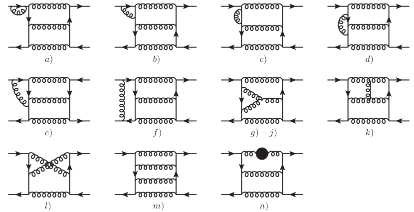
Figure 1: The relevant Feynman diagrams for the forward-scattering amplitude of $Q\overline{Q}({}^{3}S_{1}^{(1)})\to Q\overline{Q}({}^{3}S_{1}^{(1)})$ at ${\cal O}(\alpha_{s}^{4})$. It is tacitly understood that a Custkosky cut should be placed on all possible intermediate state for each diagram, since we are only interested in the imaginary part of the amplitude. We follow the same classification convention as Ref. Mackenzie:1981sf . The solid blob in class $n)$ signifies the one-loop vacuum polarization diagrams that are composed of gluon and massless quarks.

Throughout the work, we choose Feynman gauge to compute the quark amplitude, and adopt the dimensional regularization to regularize both UV and IR divergences. We use the package FeynArts Hahn:2000kx to generate Feynman diagrams and the corresponding $Q\overline{Q}$ amplitudes. As illustrated in Fig. 1, all Feynman diagrams are categorized into a dozen of groups with distinct topology. The Cutkosky’s cut is implicitly assumed and acts on all possible places. For each side of the cut, we apply the spin/color projector (7) together with (8), (9) and (10) to project out the amplitude for $Q\overline{Q}({}^{3}S_{1})$ transitioning into massless partons through $\mathcal{O}(v^{2})$. The packages FeynCalc Mertig:1990an and Form Kuipers:2012rf /FormLink Feng:2012tk are utilized for tensor contraction to obtain the squared $S$-wave amplitudes.

We utilize the packages Apart Feng:2012iq to conduct partial fraction and FIRE Smirnov:2014hma for the corresponding IBP reduction. We end up with obtaining 17 MIs for the real corrections and 58 MIs for the virtual corrections. For all the MIs, we use the packages FIESTA Smirnov:2013eza /SecDec Carter:2010hi to perform sector decomposition (SD) . For each decomposed sector, we first use CubPack CubPack /Cuba Hahn:2004fe to conduct the first-round rough numerical integration. For those integrals with large estimated errors, a parallelized integrator HCubature HCubature is utilized to repeat the numerical integration until the prescribed accuracy is achieved.

Both UV and IR divergences could arise in the NLO correction calculation. The UV divergence is affiliated only to the virtual correction calculation. We implement the on-shell renormalization for the heavy quark wave function and mass, and renormalize the strong coupling constant under $\overline{\rm MS}$ prescription. The virtual correction then becomes UV finite after standard renormalization procedure. Nevertheless, both virtual and real corrections are still plagued with IR divergences. At $\mathcal{O}(\alpha_{s}v^{0})$, upon summing both contributions, the IR divergences are exactly cancelled Mackenzie:1981sf . As we shall see in Section IV, a peculiar pattern actually emerges at $\mathcal{O}(\alpha_{s}v^{2})$. Upon summing virtual and real corrections, the IR singularities do not exactly cancel away, but leave a logarithmic IR divergence as the remnant. This single IR pole should in fact be factored into the NRQCD matrix element, so that one finally arrives at IR-finite yet scale-dependent SDC at ${\cal O}(\alpha_{s}v^{2})$.

Some remarks are in order for treating the multi-body phase space integration. Rather than directly integrating the squared amplitudes over the three(four)-body phase space, which appears to be a daunting task, we employ some modern technique, e.g., the reverse unitarity method Anastasiou:2002yz ; Gehrmann-DeRidder:2003pne to simplify the calculation. The trick is to convert a phase-space integral into a loop integral, which is facilitated by the following identity involving the $i$-th cut propagator:

$$\int\!\!\frac{d^{D}k_{i}}{(2\pi)^{D}}2\pi\,i\,\delta(k_{i}^{2})\theta(k_{i}^{0})=\int\!\!\frac{d^{D}k_{i}}{(2\pi)^{D}}\left(\frac{1}{k_{i}^{2}+i\varepsilon}-\frac{1}{k_{i}^{2}-i\varepsilon}\right).$$ (13)

Since the differentiation operation is insensitive to the $\pm i\varepsilon$ in the propagator, one can fruitfully apply the integration-by-parts (IBP) identities, which are widely used in reducing the multi-loop integrals into a set of simpler Master Integrals (MIs), also to reduce the various phase-space integrals into a set of simple MIs. We then perform the corresponding multi-body phase space integration numerically with these much simpler MIs. In Appendix A, we provide some details on how to parameterize the multi-body phase space integration in dimensional regularization.

IV Numerical results for NRQCD SDCs

In this section, we collect the known results of various SDCs in the NRQCD factorization formula for $J/\psi(\Upsilon)$ hadronic decay, and report the major new result of this work, the ${\cal O}(\alpha_{s}v^{2})$ correction to SDC.

IV.1 Leading-order NRQCD SDC

At LO in $\alpha_{s}$, the inclusive hadronic decay of the $Q\overline{Q}(^{3}S_{1})$ pair is characterized by its annihilation into three gluons. It is a straightforward exercise to deduce the LO decay rate in $d=4-2\epsilon$ spacetime dimensions:

$$\Gamma^{(0,0)}(Q\overline{Q}(^{3}S_{1})\to 3g) = \frac{1}{3}\frac{8(4E^{2})^{-1-2\epsilon}\alpha_{s}^{3}(4\pi)^{2\epsilon}}{\Gamma(2-2\epsilon)}\bigg{[}\frac{20(\pi^{2}-9)}{27}$$ (14)

$$+ \frac{5}{36}\bigg{(}28+224\zeta(3)-29\pi^{2}\bigg{)}\epsilon\bigg{]}.$$

We have introduced the symbol $\Gamma^{(i,j)}$ to denote the perturbative decay rate computed at a specific order in $\alpha_{s}$ and $v$ expansion, e.g., with the superscript $(i,j)$ signifying the joint ${\cal O}(\alpha_{s}^{i}v^{2j})$ correction. For future usage, we have deliberately kept the ${\cal O}(\epsilon)$ piece in (14).

Substituting (14) and (12a) into (4), and setting $\epsilon\to 0$, we then solve the SDC at ${\cal O}(\alpha_{s}^{0}v^{0})$:

$$F_{1}^{(0)}({}^{3}S_{1}) = \frac{20\alpha_{s}^{3}}{243m_{Q}^{2}}\left(\pi^{2}-9\right).$$ (15)

In deriving this, we have replaced $E$ by $m_{Q}$, which is valid at LO in $v^{2}$. As expected, we have just reproduced the classical result Mackenzie:1981sf ; Bodwin:1994jh ; Bodwin:2013zu .

IV.2 SDC at $\mathcal{O}(\alpha_{s}^{0}v^{2})$

Following the shortcut to extract the relativistic correction, as outlined in Section III.1, we find the $\mathcal{O}(\alpha_{s}^{0}v^{2})$ correction to the perturbative decay rate to be

$$\Gamma^{(0,1)}(Q\overline{Q}(^{3}S_{1})\to 3g) = \Gamma^{(0,0)}(Q\overline{Q}(^{3}S_{1})\to 3g){{\bm{q}}^{2}\over E^{2}}\frac{24-7\pi^{2}}{12(\pi^{2}-9)}.$$ (16)

To determine the SDC $G_{1}$, we need also expand $E$ in (16) to first order in $\tfrac{{\bm{q}}^{2}}{m_{Q}^{2}}$. Substituting (16) and (12b) into (4), with the aid of the known LO SDC $F_{1}^{(0)}$ in (15), we then deduce the SDC at ${\cal O}(\alpha_{s}^{0}v^{2})$:

$$G_{1}^{(0)}({}^{3}S_{1}) = F_{1}^{(0)}({}^{3}S_{1})\bigg{[}\frac{24-7\pi^{2}}{12(\pi^{2}-9)}-1\bigg{]}=F_{1}^{(0)}({}^{3}S_{1})\frac{132-19\pi^{2}}{12(\pi^{2}-9)},$$ (17)

which agrees with Refs. Keung:1982jb ; Bodwin:1994jh ; Bodwin:2013zu .

IV.3 SDC at $\mathcal{O}(\alpha_{s}v^{0})$

The QCD radiative correction to the vector quarkonia hadronic decay, yet at LO in velocity expansion, was first computed by Mackenzie and Lepage nearly forty years ago Mackenzie:1981sf . Dividing all the cut diagrams into several groups of distinct topology, the authors of  Mackenzie:1981sf tabulate the numerical result of each individual class of diagrams, some of which have rather limited accuracy. In order to make a close comparison with their result, we also adopt the same classification convention of Feynman diagrams as Mackenzie:1981sf .

Table 1: $\mathcal{O}(\alpha_{s}v^{0})$ contribution to the $\Gamma^{(1,0)}/(\alpha_{s}\Gamma^{(0,0)}/\pi)$ from each class of cut diagrams, with our results juxtaposed with the counterparts given in Mackenzie:1981sf . We have shifted the ’t Hooft unit mass according to $\mu^{2}\to\mu^{2}e^{\gamma_{E}}/(4\pi)$, which is equivalent to renormalizing $\alpha_{s}$ in the $\overline{\rm MS}$ scheme. For simplicity, we temporarily set the renormalization scale $\mu_{R}=2E$.

Cut diagrams	Virtual corr.	Real corr.	Real+Virtual Corr.	Result from Mackenzie:1981sf
$a$)	$-\frac{2}{\epsilon}-5.439$	—	$-\frac{2}{\epsilon}-5.439$	$-\frac{2}{\epsilon}-5.439$
$b$)	$-\frac{1}{6\epsilon}-0.726$	—	$-\frac{1}{6\epsilon}-0.726$	$-\frac{1}{6\epsilon}-(0.726\pm 0.002)$
$c$)	$-\frac{4}{3\epsilon}-0.802$	—	$-\frac{4}{3\epsilon}-0.802$	$-\frac{4}{3\epsilon}-(0.802\pm 0.002)$
$d$)	$-\frac{1}{12\epsilon}-0.142$	—	$-\frac{1}{12\epsilon}-0.142$	$-\frac{1}{12\epsilon}-(0.143\pm 0.001)$
$e$)	$0.596$	—	$0.596$	$0.594\pm 0.002$
$f$)	$\frac{4}{3\epsilon}-8.562$	—	$\frac{4}{3\epsilon}-8.562$	$\frac{4}{3\epsilon}-(8.576\pm 0.022)$
$g$)-$j$)	$\frac{4.216}{\epsilon}-17.682$	$\frac{2.534}{\epsilon}+21.318$	$\frac{6.75}{\epsilon}+3.636$	$\frac{6.75}{\epsilon}+3.54(30)$
$k$)	$-\frac{4.5}{\epsilon^{2}}-\frac{8.767}{\epsilon}+13.921$	$\frac{4.5}{\epsilon^{2}}+\frac{8.767}{\epsilon}-3.461$	$10.460(7)$	$10.59\pm 0.26$
$l$)	-3.025	—	-3.025	$-3.02\pm 0.04$
$m$)	—	-0.181	-0.181	$-0.19\pm 0.04$
$n$)	0	$\frac{3.75-0.5n_{f}}{\epsilon}$	$\frac{1.75}{\epsilon}+7.953$	$\frac{1.75}{\epsilon}+(7.96\pm 0.02)$
		$+15.327-1.844n_{f}$
C. T. ($\delta\alpha_{s}$)	$\frac{2{\rm n_{f}}-33}{4\epsilon}$	—	$\frac{2n_{f}-33}{4\epsilon}$	$\frac{2n_{f}-33}{4\epsilon}$
Total	$\frac{4.5}{\epsilon^{2}}-\frac{15.05-0.5n_{f}}{\epsilon}$	$\frac{4.5}{\epsilon^{2}}+\frac{15.05-0.5n_{f}}{\epsilon}$	$11.14(2)-1.844n_{f}$
	$-21.862(9)$	$33.003(7)-1.844n_{f}$	$3.77(2)$($n_{f}=4$)	$3.79\pm 0.53$

In Table 1, we tabulate the numerical value of $\Gamma^{(1,0)}/(\alpha_{s}\Gamma^{(0,0)}/\pi)$ for each class of cut diagrams. Following Mackenzie:1981sf , we also include in the class $c$) the diagrams with insertion of heavy quark mass counterterm. Moreover, the entry “C. T. ($\delta\alpha_{s}$)” in Table 1 signifies those tree diagrams with insertion of the counterterm for the strong coupling constant. The results from Ref. Mackenzie:1981sf are also juxtaposed with our results, which employed the gluon mass $\lambda$ to regularize IR divergences. To expedite the comparison, we replace $\log\lambda^{2}/m_{Q}^{2}$ in Mackenzie:1981sf with $1/\epsilon_{\rm IR}+\log\mu^{2}/m_{Q}^{2}$. As can be clearly observed from the Table 1, we find perfect agreement between our and their results for each class of cut diagrams. Since we are equipped with the modern IBP method tailored for multi-loop (multi-body phase space) integrals and the more accurate non-Monte-Carlo integrator, it is conceivable that a much better numerical accuracy can be achieved with respect to that in Mackenzie:1981sf .

Summing up the contributions from each class of cut diagrams, we end up with the IR-finite $\mathcal{O}(\alpha_{s}v^{0})$ correction to the perturbative decay rate:

$$\Gamma^{(1,0)}(Q\overline{Q}(^{3}S_{1})\to 3g)=\Gamma^{(0,0)}(Q\overline{Q}(^{3}S_{1})\to 3g)\frac{\alpha_{s}}{\pi}\bigg{[}\frac{3}{4}\beta_{0}\ln\frac{\mu_{R}^{2}}{4E^{2}}+11.14(2)-1.8436n_{f}\bigg{]},$$ (18)

where $\beta_{0}=11/3C_{A}-2/3n_{f}$ denotes the one-loop coefficient of the QCD $\beta$ function, with $n_{f}$ signifying the number of the active light flavors. In this work, we take $n_{f}=3$ for $J/\psi$ decay and $n_{f}=4$ for $\Upsilon$ decay. $\mu_{R}$ in (18) represents the renormalization scale, whose explicit occurrence is demanded by the renormalization group invariance.

Substituting (18) and (12a) into (4), setting $E=m_{Q}$, we then deduce the SDC at ${\cal O}(\alpha_{s}^{0}v^{0})$:

$$F_{1}^{(1)}({}^{3}S_{1})=F_{1}^{(0)}({}^{3}S_{1})\frac{\alpha_{s}}{\pi}\left[\frac{3}{4}\beta_{0}\ln\frac{\mu_{R}^{2}}{4m_{Q}^{2}}+11.14(2)-1.8436n_{f}\right],$$ (19)

which is compatible with the result in literature Mackenzie:1981sf ; Bodwin:1994jh ; Bodwin:2013zu , yet bears a much smaller error.

IV.4 SDC at $\mathcal{O}(\alpha_{s}v^{2})$

We proceed to determine the numerical value of $G_{1}^{(1)}({}^{3}S_{1})$, by far the unknown SDC at $\mathcal{O}(\alpha_{s}v^{2})$.

Table 2: $\mathcal{O}(\alpha_{s}v^{2})$ contribution to the $\Gamma^{(1,1)}/(\alpha_{s}v^{2}\Gamma^{(0,0)}/\pi)$ from each class of cut diagrams. We have set the scale affiliated with dimensional regularization to be $\mu=2E$.

. Cut diagrams Virtual corr. Real corr. Virtual+Real corrs. $a$) $\frac{8.641}{\epsilon}+{33.777}$ — $\frac{8.641}{\epsilon}+{33.777}$ $b$) $\frac{0.720}{\epsilon}+{1.797}$ — $\frac{0.720}{\epsilon}+{1.797}$ $c$) $\frac{5.761}{\epsilon}+{5.992}$ — $\frac{5.761}{\epsilon}+{5.992}$ $d$) $\frac{0.360}{\epsilon}+{0.699}$ — $\frac{0.360}{\epsilon}+{0.699}$ $e$) $-1.570$ — $-1.570$ $f$) $-\frac{3.983}{\epsilon}+{26.390}$ — $-\frac{3.983}{\epsilon}+{26.390}$ $g)$-$j$) $-\frac{3.700}{\epsilon^{2}}-\frac{27.095}{\epsilon}+{42.489}$ $\frac{3.700}{\epsilon^{2}}-\frac{2.070}{\epsilon}-{125.918}$ $-\frac{29.164}{\epsilon}-{83.429}$ $k$) $\frac{23.143}{\epsilon^{2}}+\frac{77.197}{\epsilon}+{123.118}$ $-\frac{23.143}{\epsilon^{2}}-\frac{77.196}{\epsilon}-{140.976}$ $-{17.857}$ $l$) $11.793$ — $11.793$ $m$) — $4.272$ $4.272$ $n$) — $\frac{2.160n_{f}-16.202}{\epsilon}$ $\frac{2.160n_{f}-16.202}{\epsilon}$ $+9.392n_{f}-76.924$ $+9.392n_{f}-76.924$ C. T. $\frac{-2.160n_{f}+35.645}{\epsilon}$ — $\frac{-2.160n_{f}+35.645}{\epsilon}$ ($\delta\alpha_{s}$) $-3.069n_{f}+50.636$ — $-3.069n_{f}+50.636$ Total $\frac{19.443}{\epsilon^{2}}+\frac{-2.160n_{f}+97.247}{\epsilon}$ $-\frac{19.443}{\epsilon^{2}}+\frac{2.160n_{f}-95.469}{\epsilon}$ $\frac{16}{9\epsilon}$ $-3.069n_{f}+295.121(3)$ $+9.3923n_{f}-339.545(6)$ $+6.3235n_{f}-44.424(6)$

In Table 2, we tabulate the individual contribution from each class of cut diagrams to the perturbative hadronic decay rate. The numbering convention for the Feynman diagrams is the same as Table 1. Upon summing all the individual contribution in Table 2, and implementing standard renormalization procedure, we obtain the following inclusive decay rate in QCD side at $\mathcal{O}(\alpha_{s}v^{2})$:

$$\Gamma^{(1,1)}\left(Q\bar{Q}(^{3}S_{1})\to 3g\right) = \Gamma^{(0,0)}(Q\bar{Q}(^{3}S_{1})\to 3g)\frac{\alpha_{s}v^{2}}{\pi}\bigg{[}\frac{24-7\pi^{2}}{12(\pi^{2}-9)}\frac{3}{4}\beta_{0}\ln\frac{\mu_{R}^{2}}{4E^{2}}$$ (20)

$$+ \frac{16}{9}\left({1\over\epsilon_{\rm IR}}+\ln\frac{\mu_{\Lambda}^{2}}{4E^{2}}\right)-44.424(6)+6.3235n_{f}\bigg{]}.$$

Clearly, the occurrence of $G_{1}^{(0)}({}^{3}S_{1})\beta_{0}\ln\mu_{R}$ reflects the $\mu_{R}$-independence of the decay rate, which is demanded by the standard renormalization group equation.

A salient trait in (20) is the occurrence of an uncancelled single IR pole. We assign the symbol $\mu_{\Lambda}$ to denote the scale accompanied with this single IR pole, which has very different origin from the QCD renormalization scale $\mu_{R}$.

The uncanceled single IR pole in (20), which arises at the hard region at ${\cal O}(\alpha_{s}v^{2})$, is actually not surprising at all. In fact, this symptom was first discovered in the ${\cal O}(\alpha_{s}v^{2})$ corrections for $J/\psi\to e^{+}e^{-}$ Luke:1997ys (see also Bodwin:2008vp ), $\eta_{c}\to\gamma\gamma$ Jia:2011ah , $J/\psi\to 3\gamma$ Feng:2012by , and $\eta_{c}$ total hadronic width Guo:2011tz . Physically, this unremoved IR pole indicates the breakdown of the color transparency once beyond the LO in $v$. This IR divergence can be factored in the renormalized NRQCD matrix element, so that the ${\cal O}(\alpha_{s}v^{2})$ SDC will explicitly depend on the NRQCD factorization scale $\mu_{\Lambda}$, which naturally ranges from $m_{Q}v$ to $m_{Q}$.

Expanding $E$ in (20) around $m_{Q}$ in power series of ${\bm{q}}^{2}/m_{Q}^{2}$, then comparing (20) with (4), we finally obtain the desired SDC in $\overline{\rm MS}$ factorization scheme:

$$G_{1}^{(1)}({}^{3}S_{1}) = F_{1}^{(0)}({}^{3}S_{1})\frac{\alpha_{s}}{\pi}\bigg{[}\frac{132-19\pi^{2}}{12(\pi^{2}-9)}\frac{3}{4}\beta_{0}\ln\frac{\mu_{R}^{2}}{4m_{Q}^{2}}+\frac{16}{9}\ln\frac{\mu_{\Lambda}^{2}}{4m_{Q}^{2}}$$ (21)

$$- 63.82(2)+8.6671n_{f}\bigg{]}.$$

Equation (21) constitutes the major new finding of this work. It is interesting to note that the SDC at ${\cal O}(\alpha_{s}v^{2})$ contains the same $\ln\mu_{\Lambda}$ term as the case for $J/\psi\to 3\gamma$ Feng:2012by . However, (21) also contains a negative non-logarithmic constant, in sharp contrast with what is found for $J/\psi\to 3\gamma$ Feng:2012by .

V Phenomenological analysis 

Having all the SDCs through ${\cal O}(\alpha_{s})$ at hand, we are ready to conduct a detailed phenomenological analysis based on the NRQCD factorization formula (1).

V.1 Phenomenology for $J/\psi(\Upsilon)\to{\rm LH}$ 

Before launching into concrete numerics, we would like to first develop some intuition on the relative importance of the various corrections. Setting $\mu_{R}=\mu_{\Lambda}=m_{Q}$, we then obtain

$$\Gamma[J/\psi\to{\rm LH}]=0.0716\frac{\alpha_{s}^{3}\langle\mathcal{O}_{1}({}^{3}S_{1})\rangle_{J/\psi}}{m_{c}^{2}}\bigg{[}1-5.32\langle v^{2}\rangle_{J/\psi}-1.19\alpha_{s}+3.03\alpha_{s}\langle v^{2}\rangle_{J/\psi}\bigg{]},$$ (22a)

$$\Gamma[\Upsilon\to{\rm LH}]=0.0716\frac{\alpha_{s}^{3}\langle\mathcal{O}_{1}({}^{3}S_{1})\rangle_{\Upsilon}}{m_{b}^{2}}\bigg{[}1-5.32\langle v^{2}\rangle_{\Upsilon}-1.56\alpha_{s}+4.61\alpha_{s}\langle v^{2}\rangle_{\Upsilon}\bigg{]}.$$ (22b)

To condense the notation, we have introduced the dimensionless ratio $\langle v^{2}\rangle_{V}$ to characterize the relativistic correction:

$$\langle v^{2}\rangle_{V}\equiv\frac{\langle 0|\chi^{\dagger}{\bm{\sigma}}\cdot{\bm{\epsilon}}^{\ast}\big{(}-\tfrac{i}{2}\overleftrightarrow{\bf{D}}\big{)}^{2}\psi|V\rangle}{m_{Q}^{2}\langle 0|\chi^{\dagger}\bm{\sigma}\cdot\bm{\epsilon}^{\ast}\psi|V\rangle}.$$ (23)

To make concrete predictions, we need further specify various input parameters: the value of heavy quark masses, various NRQCD matrix elements, as well as the running strong coupling constant evaluated around the quarkonium mass. We choose the quark pole mass to be $m_{c}=1.4$ GeV and $m_{b}=4.6$ GeV Feng:2012by . We take the same value of NRQCD matrix elements for $J/\psi$ as in Ref. Bodwin:2007fz :

$$\langle\mathcal{O}_{1}({}^{3}S_{1})\rangle_{J/\psi}=0.446\;{\rm GeV}^{3},\qquad\quad\langle v^{2}\rangle_{J/\psi}=0.223.$$ (24)

We also take the values of the NRQCD matrix elements for $\Upsilon(nS)$ from Ref. Chung:2010vz  :

$$\langle\mathcal{O}_{1}({}^{3}S_{1})\rangle_{\Upsilon(1S)} = 3.069\;{\rm GeV}^{3},\qquad\quad\langle v^{2}\rangle_{\Upsilon(1S)}=-0.009\pm 0.003,$$ (25a)

$$\langle\mathcal{O}_{1}({}^{3}S_{1})\rangle_{\Upsilon(2S)} = 1.623\;{\rm GeV}^{3},\qquad\quad\langle v^{2}\rangle_{\Upsilon(2S)}=0.09.$$ (25b)

We use the package RunDec Chetyrkin:2000yt to compute the QCD running coupling constant to two-loop accuracy:

$$\alpha_{s}(m_{c})=0.36,\qquad\alpha_{s}(m_{b})=0.22.$$ (26)

Table 3: NRQCD predictions to $J/\psi(\Upsilon(nS)\to{\rm LH}$ at various level of accuracy in $\alpha_{s}$ and $v$, by setting $\mu_{R}=\mu_{\Lambda}=m_{Q}$. The last column lists the measured values taken from PDG 2020 Zyla:2020zbs .

	LO	$\mathcal{O}(v^{2})$	$\mathcal{O}(\alpha_{s})$	$\mathcal{O}(\alpha_{s}v^{2})$	Total	Exp. Zyla:2020zbs
$J/\psi$	$767$	$-910$	$-330$	$187$	$-286$	$59.5\pm 2.7$
$\Upsilon(1S)$	$108$	$5$	$-37$	$-1$	$75$	$44.1\pm 1.4$
$\Upsilon(2S)$	$57$	$-27$	$-19$	$5$	$15$	$18.8\pm 2.0$

Our predictions for the hadronic widths of $J/\psi$ and $\Upsilon(1S,2S)$ are tabulated in Table 3. One readily observes that the $\mathcal{O}(\alpha_{s}v^{2})$ corrections are moderate in magnitude with respect to $\mathcal{O}(\alpha_{s}^{0}v^{2})$ and $\mathcal{O}(\alpha_{s}v^{0})$ corrections, which may indicate that NRQCD expansion exhibits reasonable convergence behavior both in $\alpha_{s}$ and $v$ in these channels. It is interesting to remark that, this pattern is in sharp contrast with the situation for $J/\psi\to 3\gamma$, where one encounters a very significant positive $\mathcal{O}(\alpha_{s}v^{2})$ correction!

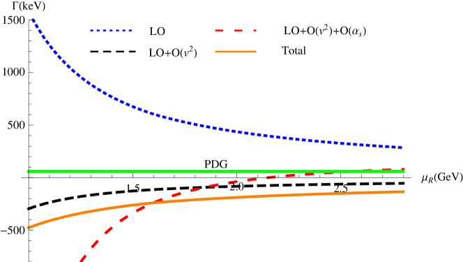
Figure 2: Predicted hadronic width of $J/\psi$ (in unit of keV) as a function of the renormalization scale $\mu_{R}$ by holding the NRQCD factorization scale fixed, $\mu_{\Lambda}=m_{c}$. Different curves designate the various predictions at various levels of accuracy in $\alpha_{s}$ and $v$ expansion.

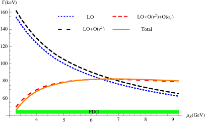
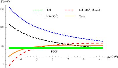
Figure 3: Predicted decay rate for $\Upsilon(1S)\to{\rm LH}$ as a function of $\mu_{R}$ at various levels of accuracy in NRQCD expansion, with $\mu_{\Lambda}=m_{b}$. For the plot on the left panel, we take the value of $\langle v^{2}\rangle_{\Upsilon(1S)}$ same as in (25a), while on the right panel we take $\langle v^{2}\rangle_{\Upsilon(1S)}=0.056$ in (27), which is determined through G-K relation.

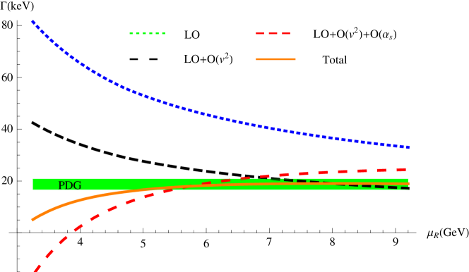
Figure 4: Predicted decay rate for $\Upsilon(2S)\to{\rm LH}$ as a function of $\mu_{R}$ at various levels of accuracy in NRQCD expansion, with $\mu_{\Lambda}=m_{b}$.

As one easily recognizes from Table 3, a salient feature for $J/\psi\to{\rm LH}$ is the disquietingly negative $\mathcal{O}(\alpha_{s}^{0}v^{2})$ correction, which is even greater than LO prediction in magnitude. Even worse, the $\mathcal{O}(\alpha_{s}v^{0})$ radiative correction further decreases the predicted hadronic width. Although the new $\mathcal{O}(\alpha_{s}v^{2})$ correction tends to increase the prediction, unfortunately its effect is not significant enough to bring the predicted hadronic width to a positive value, so that we are unable to make a meaningful prediction to confront the measurement.

To closely examine this apparent discrepancy between theory and experiment, we further display in Fig. 2 the dependence of $J/\psi$ hadronic decay rate on the renormalization scale $\mu_{R}$ at various level of accuracy in $\alpha_{s}$ and $v$ expansion, with the NRQCD factorization scale $\mu_{\Lambda}=m_{c}$ held fixed. In the reasonable range of $1\;{\rm GeV}<\mu_{R}<2m_{c}$, we again observe that the total decay rate is always negative. As mentioned before, the root of this dilemma can be readily traced from (22a), that is, mainly due to the substantially negative $\mathcal{O}(\alpha_{s}^{0}v^{2})$ and $\mathcal{O}(\alpha_{s}v^{0})$ corrections and moderately positive $\mathcal{O}(\alpha_{s}v^{2})$ correction. Thus, we conclude that the state-of-the-art NRQCD prediction ceases to yield a physically meaningful result for $J/\psi\to{\rm LH}$. How to account for the experimental data from the perspective of NRQCD factorization remains an open challenge. As a potentially appealing solution, one may conjecture that the uncalculated ${\cal O}(\alpha_{s}^{2}v^{0})$ correction might be significantly positive, which would bring the NRQCD prediction closer to measured value. Unfortunately, the bottleneck of the current multi-loop(leg) calculational capability impedes one to tackle this type of NNLO perturbative correction in the foreseeable future.

From Table 3, one observes that the ${\cal O}(\alpha_{s}v^{2})$ correction has rather minor effect for $\Upsilon(1S,2S)\to{\rm LH}$, much less significant than the ${\cal O}(\alpha_{s}v^{0})$ and ${\cal O}(\alpha_{s}^{0}v^{2})$ corrections. In Fig. 3 and Fig. 4, the hadronic decay rates of $\Upsilon(1S,2S)$ are displayed as a function of the renormalization scale $\mu_{R}$. As can be easily visualized, though the LO NRQCD prediction exhibits strong $\mu_{R}$ dependence, after including the corrections through ${\cal O}(\alpha_{s}v^{2})$, the decay rate becomes much less sensitive to the variation of $\mu_{R}$, especially when $\mu_{R}>m_{b}$.

The relativistic corrections in $\Upsilon(1S)$ hadronic decay appear to be negligible, which can be attributed to the highly suppressed relativistic NRQCD matrix elements, as clearly seen in (25a). We choose two different values for the relativistic NRQCD matrix element to make predictions for $\Upsilon(1S)\to{\rm LH}$. When choosing the values specified in (25a), the finest NRQCD prediction for $\Upsilon(1S)$ hadronic width is considerably larger than the measured value, which can be readily seen in Table 3 and the left panel of Fig. 3.

Alternatively, one can estimate the $\langle v^{2}\rangle_{\Upsilon(1S)}$ according to the Gremm-Kapustin (G-K) relation Gremm:1997dq :

$$\langle v^{2}\rangle_{\Upsilon(1S)}\approx{M_{\Upsilon(1S)}-2m_{b}\over m_{b}}=0.056,$$ (27)

once $m_{b}=4.6$ GeV is chosen. With such choice, the $\mathcal{O}(\alpha_{s}v^{2})$ correction may reach $10\%$ of the LO decay rate. Consequently, for $m_{b}\leq\mu_{R}\leq 2m_{b}$, the hadronic width of $\Upsilon(1S)$ is predicted to be in the range $44-51\;{\rm keV}$. Interestingly, as one can tell from the right panel of Fig. 3, the finest NRQCD prediction is in satisfactory agreement with the measured value: $44.1\pm 1.4\;{\rm keV}$ Zyla:2020zbs .

For $\Upsilon(2S)$ hadronic width, both the $\mathcal{O}(\alpha_{s}v^{0})$ and $\mathcal{O}(\alpha_{s}^{0}v^{2})$ corrections are negative and sizeable. The $\mathcal{O}(\alpha_{s}v^{2})$ correction turns out to be positive, moderate in magnitude. Incorporating the new piece of $\mathcal{O}(\alpha_{s}v^{2})$ correction, the finest NRQCD prediction for the hadronic width is in the range $15-19\;{\rm keV}$ for $m_{b}\leq\mu_{R}\leq 2m_{b}$, compatible with the measured value $18.8\pm 2.0\;{\rm keV}$ Zyla:2020zbs .

V.2 Phenomenology for $J/\psi(\Upsilon)\to 3\gamma$ 

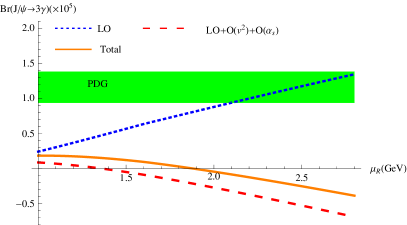
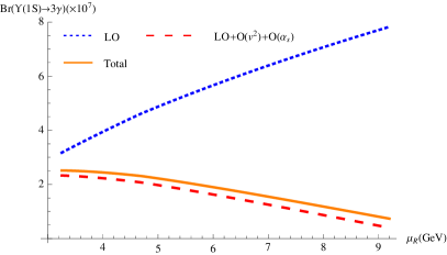
Figure 5: NRQCD predictions for the branching fractions of $J/\psi\to 3\gamma$ (left panel) and $\Upsilon(1S)\to 3\gamma$ (right panel) with various levels of accuracy in $\alpha_{s}$ and $v$ expansion, with $\mu_{\Lambda}$ fixed to be heavy quark mass. The rare electromagnetic decay $\Upsilon\to 3\gamma$ has not yet been observed experimentally. We take $\langle v^{2}\rangle_{\Upsilon(1S)}=0.056$ in (27), which is inferred from G-K relation.

The knowledge of the ${\cal O}(\alpha_{s}v^{2})$ correction enables us not only to present the most complete NRQCD predictions for hadronic widths of vector quarkonia, but present the finest NRQCD predictions for the rare electromagnetic decay $J/\psi(\Upsilon)\to 3\gamma$.

The ${\cal O}(\alpha_{s}v^{2})$ corrections to the partial width of $J/\psi(\Upsilon)\to 3\gamma$ were addressed by the authors some time ago Feng:2012by :

$$\Gamma(V\to 3\gamma) = \frac{8(\pi^{2}-9)e_{Q}^{6}\alpha^{3}}{9m_{Q}^{2}}\langle\mathcal{O}_{1}({}^{3}S_{1})\rangle_{V}\bigg{\{}1-12.630\frac{\alpha_{s}}{\pi}$$

$$+ \bigg{[}\frac{132-19\pi^{2}}{12(\pi^{2}-9)}+\bigg{(}\frac{16}{9}\ln\frac{\mu_{\Lambda}^{2}}{m_{Q}^{2}}+68.913\bigg{)}\frac{\alpha_{s}}{\pi}\bigg{]}\langle v^{2}\rangle_{V}\bigg{\}},$$

where $e_{Q}$ represents the electric charge of the heavy quark, and $\alpha$ denotes the fine structure constant. Curiously, the $\ln\mu_{\Lambda}$ term in the ${\cal O}(\alpha_{s}v^{2})$ SDC is identical to that in $G_{1}^{(1)}({}^{3}S_{1})$ in (21).

Dividing (V.2) by (1), and plugging the result for various SDCs through ${\cal O}(\alpha_{s}v^{2})$ that are tabulated in Section IV, we then obtain the state-of-the-art NRQCD predictions for the branching fractions of $J/\psi(\Upsilon)\to 3\gamma$. In the spirit of NRQCD expansion, we further expand the ratio in power series of $\alpha_{s}$ and $v^{2}$ and obtain

$${\rm Br}(J/\psi\to 3\gamma) = {\rm Br}(J/\psi\to{\rm LH})\times{\Gamma(J/\psi\to 3\gamma)\over\Gamma(J/\psi\to{\rm LH})}$$

$$= 0.641\frac{\alpha^{3}}{\alpha_{s}^{3}}\bigg{[}0.948-\frac{\alpha_{s}}{\pi}\bigg{(}8.42+6.40\ln\frac{\mu_{R}^{2}}{m_{c}^{2}}\bigg{)}+\frac{\alpha_{s}}{\pi}\langle v^{2}\rangle_{J/\psi}\;11.51\bigg{]},$$

$${\rm Br}(\Upsilon(1S)\to 3\gamma) = {\rm Br}(\Upsilon\to{\rm LH})\times{\Gamma(\Upsilon\to 3\gamma)\over\Gamma(\Upsilon\to{\rm LH})}$$

$$= 0.817\frac{\alpha^{3}}{\alpha_{s}^{3}}\bigg{[}0.0148-\frac{\alpha_{s}}{\pi}\bigg{(}0.115+0.093\ln\frac{\mu_{R}^{2}}{m_{b}^{2}}\bigg{)}+\frac{\alpha_{s}}{\pi}\langle v^{2}\rangle_{\Upsilon(1S)}\;0.197\bigg{]}.$$

To reduce the theoretical error, we take ${\rm Br}(J/\psi\to{\rm LH})=64.1\%$ and ${\rm Br}(\Upsilon(1S)\to{\rm LH})=81.7\%$ as experimental input Zyla:2020zbs .

As is evident in (29), The LO NRQCD matrix element has canceled in the ratio. More interestingly, the ${\cal O}(\alpha_{s}^{0}v^{2})$ correction has also completely disappear in the ratio. Furthermore, the explicit logarithmic dependence on NRQCD factorization scale $\mu_{\Lambda}$ has also disappeared.

In Fig. 5 we display our predictions for the branching fractions of $J/\psi\to 3\gamma$ (left panel) and $\Upsilon(1S)\to 3\gamma$ (right panel) at various levels of accuracy in $\alpha_{s}$ and $v$ expansion, with $\mu_{\Lambda}=m_{Q}$. The sensitivity of the branching fractions to $\mu_{R}$ seems not to improve much after incorporating the higher order corrections. This may be attributed to the sizeable radiative corrections and the $\alpha_{s}^{3}$ factor in the denominator. Setting $\mu_{R}=m_{c}$, the finest NRQCD prediction is ${\rm Br}(J/\psi\to 3\gamma)=1.45\times 10^{-6}$, about one order of magnitude smaller than the measured value $1.16\times 10^{-5}$. As can be seen in Fig. 5, varying the renormalization scale in the range $1\;{\rm GeV}\leq\mu_{R}\leq 3\;{\rm GeV}$, we always observe that ${\rm Br}(J/\psi\to 3\gamma)$ is far smaller than the experimental measurement. The resolution to this dilemma may need call for including further higher order relativistic corrections Bodwin:2007fz , or incorporating the ${\cal O}(\alpha_{s}^{2}v^{0})$ correction. Such a study appears to be extremely challenging on technical ground, which is beyond the scope of this work.

In a similar fashion, with the aid of (29), we can predict ${\rm Br}(\Upsilon(1S)\to 3\gamma)=2.06^{+0.20}_{-1.55}\times 10^{-7}$ and ${\rm Br}(\Upsilon(2S)\to 3\gamma)=1.78^{+0.11}_{-0.99}\times 10^{-7}$, where the uncertainties are estimated by varying $\mu_{R}$ from $m_{b}/2$ to $2m_{b}$. The uncertainties looks significant due to strong $\mu_{R}$ dependence. Alternatively, if we choose $\langle v^{2}\rangle_{\Upsilon(1S)}=0.056$ as indicated by the G-K relation, the branching fraction shifts to ${\rm Br}(\Upsilon(1S)\to 3\gamma)=2.33^{+0.18}_{-1.44}\times 10^{-7}$. It is a clear sign that the relativistic effect is less important for bottomonium case, and the branching fraction appears to be insensitive to the relativistic corrections. We hope future experiments for $\Upsilon$ rare electromagnetic decay can test our predictions.

VI Summary

In summary, we have computed the ${\mathcal{O}(\alpha_{s}v^{2})}$ corrections to $J/\psi(\Upsilon)$ hadronic decays, precisely deducing the corresponding SDCs. Unlike the case in $J/\psi(\Upsilon)\to 3\gamma$, the corrections are moderate, therefore the expansion in $v^{2}$ exhibits a decent convergence behavior. We find that the theoretical predictions for the decay width of $J/\psi\to{\rm LH}$ is negative through $\mathcal{O}(\alpha_{s}v^{2})$, which is certainly unphysical and can be attributed to the sizable and negative relativistic corrections. On the other hand, we find the theoretical predictions for $\Upsilon(1S,2S)$ hadronic decays are consistent with the experimental data, if the NRQCD matrix elements $\langle v^{2}\rangle_{\Upsilon(nS)}$ are appropriately chosen. Incorporating the formulas in the Ref. Feng:2012by , we derive the branching fraction for $J/\psi(\Upsilon)\to 3\gamma$ accurate up to ${\mathcal{O}(\alpha_{s}v^{2})}$. Although the ${\mathcal{O}(v^{2})}$ relativistic corrections get exactly cancelled, we observe a strong $\mu_{R}$ dependence in the branching ratio. Once again, we find the theoretical prediction for ${\rm Br}(J/\psi\to 3\gamma)$ can not explain the experimental measurement. In our opinion, the theoretical incompetence to precisely predicting $J/\psi$ decay in NRQCD factorization approach may be attributed to the not-yet-known higher-order relativistic and perturbative corrections.

Appendix A Tactics in dealing with four-body phase space integration 

In this Appendix, we present some technical details on how we parameterize the three-particle and four-particle phase space integrals in $d$ dimensions. Our central goal is to eliminate the Heaviside step function in the four-particle phase space integration through some trick, so that we can choose some highly precise numerical integrator other than the widely-used, but less accurate, adaptive Monte Carlo integrator.

We start with the Born-order process for $J/\psi(\Upsilon)\to{\rm LH}$, where the decay product is comprised of three gluons. We define the following Lorentz invariants:

$$P\cdot k_{1}=2x_{1}E^{2},\;\;\;P\cdot k_{2}=2x_{2}E^{2},\;\;\;P\cdot k_{1}=2(2-x_{1}-x_{2})E^{2},$$ (30)

$$k_{1}\cdot k_{2}=2E^{2}(x_{1}+x_{2}-1),\;\;\;k_{1}\cdot k_{3}=2E^{2}(1-x_{2}),\;\;\;k_{2}\cdot k_{3}=2E^{2}(1-x_{1}),$$

where the momenta $P$ and $k_{i}\,(i=1,2,3)$ have been defined in Section III.1. The dimensionless variables $x_{1}$ and $x_{2}$ are constrained to be $1\leq x_{1}+x_{2}\leq 2$ by energy conservations. It is useful to change variables from $(x_{1},x_{2})$ to $(x,y)$ so that the integration range of the new variables lie in a square Petrelli:1997ge :

$$x_{1}=x,\;\;\;x_{2}=1-xy,$$ (31)

with $0\leq x,y\leq 1$.

It is then straightforward to parameterize the phase space integral of three massless particle in $d=4-2\epsilon$ space-time dimensions as

$$\int\!\!d\Phi_{3} = \int\!\!\!\frac{d^{d-1}k_{1}}{2k_{1}^{0}(2\pi)^{d-1}}\frac{d^{d-1}k_{2}}{2k_{2}^{0}(2\pi)^{d-1}}\frac{d^{d-1}k_{3}}{2k_{3}^{0}(2\pi)^{d-1}}(2\pi)^{d}\delta^{d}(P-k_{1}-k_{2}-k_{3})$$ (32)

$$=\frac{(4E^{2})^{1-2\epsilon}}{128\pi^{3}}\frac{(4\pi)^{2\epsilon}}{\Gamma(2-2\epsilon)}\int_{0}^{1}\!dx\,dy\>x^{1-2\epsilon}\bigg{[}y(1-x)(1-y)\bigg{]}^{-\epsilon}.$$

Calculation of the real corrections demands considering the $J/\psi(\Upsilon)$ decay into four massless partons. The four-particle phase space integration in dimensional regularization is somewhat intriguing. We employ the parametrization scheme introduced in Ref. GehrmannDe Ridder:2003bm . The Mandelstam variables are defined as $s_{ij}=k_{i}\cdot k_{j}$, which obey $s_{12}+s_{13}+s_{14}+s_{23}+s_{24}+s_{34}=4E^{2}$ constrained by energy conservation. It is convenient to introduce a set of dimensionless variables $x_{i}$ through rescaling the Mandelstam invariants by

$$x_{1}=\frac{s_{12}}{4E^{2}},\qquad x_{2}=\frac{s_{13}}{4E^{2}},\qquad x_{3}=\frac{s_{23}}{4E^{2}},$$

$$x_{4}=\frac{s_{14}}{4E^{2}},\qquad x_{5}=\frac{s_{24}}{4E^{2}},\qquad x_{6}=\frac{s_{34}}{4E^{2}}.$$

In terms of the dimensionless variables in (A), the massless four-body phase space can be parameterized as GehrmannDe Ridder:2003bm

$$\int\!\!d\Phi_{4} = \int\!\!\!\frac{d^{d-1}k_{1}}{2k_{1}^{0}(2\pi)^{d-1}}\frac{d^{d-1}k_{2}}{2k_{2}^{0}(2\pi)^{d-1}}\frac{d^{d-1}k_{3}}{2k_{3}^{0}(2\pi)^{d-1}}\frac{d^{d-1}k_{3}}{2k_{4}^{0}(2\pi)^{d-1}}(2\pi)^{d}\delta(P-k_{1}-k_{2}-k_{3}-k_{4})$$ (34)

$$= C_{\Gamma}(4E^{2})^{\frac{3d}{2}-4}\int_{0}^{1}\!\!\prod_{j=1}^{6}dx_{j}\delta\left(1-\sum_{i=1}^{6}{x_{i}}\right)[-\lambda(x_{1}x_{6},x_{2}x_{5},x_{3}x_{4})]^{\frac{d-5}{2}}\Theta(-\lambda),$$

where $\lambda(x,y,z)=x^{2}+y^{2}+z^{2}-2(xy+xz+yz)$ is the Källen function, $\Theta$ represents the Heaviside step function, and the volume factor $C_{\Gamma}$ is given by

$$C_{\Gamma}=(2\pi)^{4-3d}V(d-1)V(d-2)V(d-3)2^{1-2d},$$ (35)

with $V(d)=\frac{2\pi^{d/2}}{\Gamma(d/2)}$ designating the area of the unit sphere imbedded in $d$-dimensional space.

The presence of Heaviside step function in (34) generally renders the integration boundary highly irregular, so that one has to resort to the Monte Carlo recipe for numerical integration, with some intrinsic limitation on integration accuracy. In fact, we can manage to eliminate the Heaviside function through a clever trick, so that we can employ more accurate numerical integrator other than the Monte Carlo algorithm.

First let us explicitly write down the Källen function in (34), abbreviated by $\lambda$ for simplicity:

$$\lambda\equiv\lambda(x_{1}x_{6},x_{2}x_{5},x_{3}x_{4}) = x_{3}^{2}x_{4}^{2}+x_{2}^{2}x_{5}^{2}+x_{1}^{2}x_{6}^{2}-2(x_{2}x_{3}x_{4}x_{5}+x_{1}x_{2}x_{5}x_{6}+x_{1}x_{3}x_{4}x_{6}).$$

With the aid of Cheng-Wu theorem Cheng-Wu-1 ; Bjoerkevoll:1992cu ; Smirnov_Book , we have the freedom to pull the variables $x_{1}$, $x_{2}$ and $x_{3}$ outside the $\delta$-function when carrying out phase space integration (34). Consequently, the integration range of $x_{1}$, $x_{2}$ and $x_{3}$ then become $[0,\infty)$, essentially unbounded. We can freely rename the variables:

$$x_{1}\to\frac{x_{1}}{x_{6}},\quad x_{2}\to\frac{x_{2}}{x_{5}},\quad x_{3}\to\frac{x_{3}}{x_{4}}.$$ (37)

Now the Källen function reduces to

$$\lambda \to x_{1}^{2}+x_{2}^{2}+x_{3}^{2}-2(x_{1}x_{2}+x_{2}x_{3}+x_{1}x_{3})$$ (38)

$$= (x_{1}-x_{2})^{2}+x_{3}^{2}-2x_{1}x_{3}-2x_{2}x_{3}.$$

We can divide the integration range for $x_{1}$ and $x_{2}$ into two sectors: $x_{1}\geq x_{2}$ and $x_{1}<x_{2}$. For the first sector $x_{1}\geq x_{2}$, it is convenient to further change the variables:

$$x_{2}\to\frac{x_{2}}{2},\qquad x_{1}\to x_{1}+\frac{x_{2}}{2}.$$ (39)

For the second sector $x_{1}<x_{2}$, we can also make variable change:

$$x_{1}\to\frac{x_{2}}{2}\qquad x_{2}\to x_{1}+\frac{x_{2}}{2}.$$ (40)

The advantage of changing variables is to ensure that the support of the new variables are within a square, e.g., both integration ranges of new $x_{1}$ and $x_{2}$ lie in $[0,\infty)$.

Without loss of generality, we choose the first sector to illustrate our recipe. After changing variables in line with (39), the Källen function now simplifies to

$$\lambda=(x_{1}-x_{3})^{2}-2x_{2}x_{3}.$$ (41)

Similarly, we can further break the integration into two sectors: $x_{1}\geq x_{3}$ and $x_{1}<x_{3}$. For the $x_{1}\geq x_{3}$ sector, we are free to continue to rename the variables:

$$x_{3}\to\frac{x_{3}}{2}\qquad x_{1}\to x_{1}+\frac{x_{3}}{2}.$$ (42)

And for the $x_{1}<x_{3}$ sector, we change the variables as

$$x_{1}\to\frac{x_{3}}{2},\qquad x_{3}\to x_{1}+\frac{x_{3}}{2}.$$ (43)

Now the integration range of the new $x_{1}$ and $x_{3}$ variables lie in $[0,\infty)$.

We can repeat the game of dissecting the integral into two sub-sectors. For concreteness, let us concentrate on the sub-sector $x_{1}\geq x_{3}$. After changing variables as advised in (42), the Källen function now reduces to

$$\lambda=x_{1}^{2}-x_{2}x_{3}.$$ (44)

We further rename the variable $x_{2}$ as

$$x_{2}\to\frac{x_{1}x_{2}}{x_{3}},$$ (45)

so that $\lambda$ in (44) reduces to

$$\lambda=x_{1}(x_{1}-x_{2}).$$ (46)

One more again, we can dissect the integration range into two sectors: $x_{1}\geq x_{2}$ and $x_{1}<x_{2}$. As indicated by the Heaviside function $\Theta(-\lambda)$ in (34), the first sub-sector ($x_{1}\geq x_{2}$) apparently make vanishing contribution. Therefore, only the second sub-sector with $x_{1}<x_{2}$ survives. We further change the variables as follows:

$$x_{1}\to\frac{x_{2}}{2},\qquad x_{2}\to x_{1}+\frac{x_{2}}{2}.$$ (47)

So the integration range of the new $x_{1}$ and $x_{2}$ variables also lies in $[0,\infty)$. Meanwhile, the Källen function reduces to $\lambda=-\frac{x_{1}x_{2}}{2}$. Since the Heaviside function $\Theta(-\lambda)$ remains 1 in this prescribed integration support, it can be safely dropped. This sequences of manipulation can be recursively applied to any integration sector.

At the last step, we can invoke Cheng-Wu theorem again to put $x_{1}$, $x_{2}$ and $x_{3}$ back inside the $\delta$-function.

Through the aforementioned manipulations, we are able to eliminate the Heaviside $\Theta$ function from the four-particle phase space integral. Since the support of the multi-dimensional integration variables is inside a regular hypercube, we can resort to any efficient numerical integrator, e.g., the parallelized integrator HCubature HCubature for high-precision numerical integration.

As a test, we apply sector decomposition method together with our parametrization to numerically calculate five MIs of the massless four-body phase-space type (labelled by $R_{4}$, $R_{6}$, $R_{8,a}$, $R_{8,b}$ and $R_{8,r}$ in GehrmannDe Ridder:2003bm ). These five MIs have been analytically worked out in 2003 GehrmannDe Ridder:2003bm , with which we find exquisite numerical agreement.

References

- (1) T. Appelquist and H. D. Politzer, Phys. Rev. Lett. 34, 43 (1975) doi:10.1103/PhysRevLett.34.43
- (2) P. B. Mackenzie and G. P. Lepage, Phys. Rev. Lett. 47, 1244 (1981) doi:10.1103/PhysRevLett.47.1244
- (3) N. Brambilla, X. Garcia Tormo, i, J. Soto and A. Vairo, Phys. Rev. D 75, 074014 (2007) doi:10.1103/PhysRevD.75.074014 [arXiv:hep-ph/0702079 [hep-ph]].
- (4) W. E. Caswell, G. P. Lepage and J. R. Sapirstein, Phys. Rev. Lett. 38, 488 (1977) doi:10.1103/PhysRevLett.38.488
- (5) G. T. Bodwin, E. Braaten and G. P. Lepage, Phys. Rev. D 51, 1125-1171 (1995) [erratum: Phys. Rev. D 55, 5853 (1997)] doi:10.1103/PhysRevD.55.5853 [arXiv:hep-ph/9407339 [hep-ph]].
- (6) W. Y. Keung and I. J. Muzinich, Phys. Rev. D 27, 1518 (1983) doi:10.1103/PhysRevD.27.1518
- (7) G. T. Bodwin and A. Petrelli, Phys. Rev. D 66, 094011 (2002) [erratum: Phys. Rev. D 87, no.3, 039902 (2013)] doi:10.1103/PhysRevD.66.094011 [arXiv:hep-ph/0205210 [hep-ph]].
- (8) M. Butenschoen and B. A. Kniehl, Phys. Rev. D 84, 051501 (2011) doi:10.1103/PhysRevD.84.051501 [arXiv:1105.0820 [hep-ph]].
- (9) K. T. Chao, Y. Q. Ma, H. S. Shao, K. Wang and Y. J. Zhang, Phys. Rev. Lett. 108, 242004 (2012) doi:10.1103/PhysRevLett.108.242004 [arXiv:1201.2675 [hep-ph]].
- (10) Z. Sun and H. F. Zhang, Chin. Phys. C 42, no.4, 043104 (2018) doi:10.1088/1674-1137/42/4/043104 [arXiv:1505.02675 [hep-ph]].
- (11) F. Feng, Y. Jia and W. L. Sang, Phys. Rev. D 87, no.5, 051501 (2013) doi:10.1103/PhysRevD.87.051501 [arXiv:1210.6337 [hep-ph]].
- (12) M. Ablikim et al. [BESIII], Phys. Rev. D 87, no.3, 032003 (2013) doi:10.1103/PhysRevD.87.032003 [arXiv:1208.1461 [hep-ex]].
- (13) Y. Jia, Phys. Rev. D 82, 034017 (2010) doi:10.1103/PhysRevD.82.034017 [arXiv:0912.5498 [hep-ph]].
- (14) M. Beneke and V. A. Smirnov, Nucl. Phys. B 522, 321-344 (1998) doi:10.1016/S0550-3213(98)00138-2 [arXiv:hep-ph/9711391 [hep-ph]].
- (15) T. Hahn, Comput. Phys. Commun. 140, 418-431 (2001) doi:10.1016/S0010-4655(01)00290-9 [arXiv:hep-ph/0012260 [hep-ph]].
- (16) R. Mertig, M. Bohm and A. Denner, Comput. Phys. Commun. 64, 345-359 (1991) doi:10.1016/0010-4655(91)90130-D
- (17) J. Kuipers, T. Ueda, J. A. M. Vermaseren and J. Vollinga, Comput. Phys. Commun. 184, 1453-1467 (2013) doi:10.1016/j.cpc.2012.12.028 [arXiv:1203.6543 [cs.SC]].
- (18) F. Feng and R. Mertig, [arXiv:1212.3522 [hep-ph]].
- (19) F. Feng, Comput. Phys. Commun. 183, 2158-2164 (2012) doi:10.1016/j.cpc.2012.03.025 [arXiv:1204.2314 [hep-ph]].
- (20) A. V. Smirnov, Comput. Phys. Commun. 189, 182-191 (2015) doi:10.1016/j.cpc.2014.11.024 [arXiv:1408.2372 [hep-ph]].
- (21) A. V. Smirnov, Comput. Phys. Commun. 185, 2090-2100 (2014) doi:10.1016/j.cpc.2014.03.015 [arXiv:1312.3186 [hep-ph]].
- (22) J. Carter and G. Heinrich, Comput. Phys. Commun. 182, 1566-1581 (2011) doi:10.1016/j.cpc.2011.03.026 [arXiv:1011.5493 [hep-ph]].
- (23) S. Borowka and G. Heinrich, PoS LL2012, 037 (2012) doi:10.22323/1.151.0037 [arXiv:1209.6345 [hep-ph]].
- (24) F. Feng, Y. Jia and W. L. Sang, [arXiv:1901.08447 [hep-ph]].
- (25) W. L. Sang, F. Feng and Y. Jia, JHEP 10, 098 (2020) doi:10.1007/JHEP10(2020)098 [arXiv:2008.04898 [hep-ph]].
- (26) R. Cools and A. Haegemans, ACM Trans. Math. Softw. 29 (2003), no. 3 287 C296.
- (27) T. Hahn, Comput. Phys. Commun. 168, 78-95 (2005) doi:10.1016/j.cpc.2005.01.010 [arXiv:hep-ph/0404043 [hep-ph]].
- (28) https://github.com/stevengj/cubature, HCubature web site
- (29) C. Anastasiou and K. Melnikov, Nucl. Phys. B 646, 220-256 (2002) doi:10.1016/S0550-3213(02)00837-4 [arXiv:hep-ph/0207004 [hep-ph]].
- (30) A. Gehrmann-De Ridder, T. Gehrmann and G. Heinrich, Nucl. Phys. B 682, 265-288 (2004) doi:10.1016/j.nuclphysb.2004.01.023 [arXiv:hep-ph/0311276 [hep-ph]].
- (31) M. E. Luke and M. J. Savage, Phys. Rev. D 57, 413-423 (1998) doi:10.1103/PhysRevD.57.413 [arXiv:hep-ph/9707313 [hep-ph]].
- (32) G. T. Bodwin, H. S. Chung, J. Lee and C. Yu, Phys. Rev. D 79, 014007 (2009) doi:10.1103/PhysRevD.79.014007 [arXiv:0807.2634 [hep-ph]].
- (33) Y. Jia, X. T. Yang, W. L. Sang and J. Xu, JHEP 06, 097 (2011) doi:10.1007/JHEP06(2011)097 [arXiv:1104.1418 [hep-ph]].
- (34) H. K. Guo, Y. Q. Ma and K. T. Chao, Phys. Rev. D 83, 114038 (2011) doi:10.1103/PhysRevD.83.114038 [arXiv:1104.3138 [hep-ph]].
- (35) G. T. Bodwin, H. S. Chung, D. Kang, J. Lee and C. Yu, Phys. Rev. D 77, 094017 (2008) doi:10.1103/PhysRevD.77.094017 [arXiv:0710.0994 [hep-ph]].
- (36) H. S. Chung, J. Lee and C. Yu, Phys. Lett. B 697, 48-51 (2011) doi:10.1016/j.physletb.2011.01.033 [arXiv:1011.1554 [hep-ph]].
- (37) H. T. Chen, Y. Q. Chen and W. L. Sang, Phys. Rev. D 85, 034017 (2012) doi:10.1103/PhysRevD.85.034017 [arXiv:1109.6723 [hep-ph]].
- (38) K. G. Chetyrkin, J. H. Kuhn and M. Steinhauser, Comput. Phys. Commun. 133, 43-65 (2000) doi:10.1016/S0010-4655(00)00155-7 [arXiv:hep-ph/0004189 [hep-ph]].
- (39) P. A. Zyla et al. [Particle Data Group], PTEP 2020, no.8, 083C01 (2020) doi:10.1093/ptep/ptaa104
- (40) M. Gremm and A. Kapustin, Phys. Lett. B 407, 323-330 (1997) doi:10.1016/S0370-2693(97)00744-2 [arXiv:hep-ph/9701353 [hep-ph]].
- (41) A. Petrelli, M. Cacciari, M. Greco, F. Maltoni and M. L. Mangano, Nucl. Phys. B 514, 245-309 (1998) doi:10.1016/S0550-3213(97)00801-8 [arXiv:hep-ph/9707223 [hep-ph]].
- (42) A. Gehrmann-De Ridder, T. Gehrmann and G. Heinrich, “Four particle phase space integrals in massless QCD,” Nucl. Phys. B 682, 265 (2004) [hep-ph/0311276].
- (43) H. Cheng and T. T. Wu, Expanding Protons: Scattering at High Energies (MIT Press, Cambridge, MA, 1987).
- (44) V. A. Smirnov, Evaluating Feynman integrals (Springer Tracts Mod. Phys. 211, 2004), http://www.springer .com/physics/particle+and+nuclear+physics/book/978-3-540-23933-8.
- (45) K. S. Bjoerkevoll, P. Osland and G. Faeldt, Nucl. Phys. B 386, 303-342 (1992) doi:10.1016/0550-3213(92)90569-W