Categorical Wall-Crossing in Landau-Ginzburg Models

Abstract

We describe how categorical BPS data including chain complexes of solitons, CPT pairings, and interior amplitudes jump across a wall of marginal stability in two-dimensional $\mathcal{N}=(2,2)$ models. We show that our jump formulas hold if and only if the $A_{\infty}$-categories of $\frac{1}{2}$-BPS branes constructed on either side of the wall are homotopy equivalent. These results can be viewed as categorical enhancements of the Cecotti-Vafa wall-crossing formula.

1 Introduction and Outline

BPS states have played an important role in many aspects of physical mathematics. As is very well-known, the spaces of BPS states can jump discontinuously as physical parameters are varied, a phenomenon known as wall-crossing. Investigations of BPS wall-crossing have led to a wide variety of very interesting developments. For some reviews of BPS wall-crossing see [Cec, KoSo2, KoSo3, M1, N, Pio].

BPS wall-crossing appears in two-dimensional quantum field theories with $\mathcal{N}=(2,2)$ supersymmetry, where it was first discovered [CFIV, CV1] as well as in four-dimensional supergravity and field theory with $\mathcal{N}=2$ supersymmetry [DM, Dor, GMN1, LY, SW]. It also appears in a more elaborate form in coupled 2d-4d systems [GMN3].

Indeed, there are quantitative formulae expressing how BPS indices change across walls of marginal stability. It is natural to ask if one can obtain more refined information about the spaces of BPS states. For example, if BPS states are identified with the cohomology of some chain complexes one would like to know how the chain complexes themselves jump across walls of marginal stability. One cannot expect an answer at the level of chain complexes per se, since homotopy equivalent chain complexes are also physically equivalent, but it is meaningful to ask how the equivalence class of the chain complexes (up to homotopy) changes. In particular, relating the homotopy equivalence class of chain complexes across a marginal stability wall allows us, by taking cohomology, to answer How do the BPS Hilbert spaces jump across a wall of marginal stability? This is the question a categorified wall-crossing formula is meant to answer.

The present paper addresses the categorification of the renowned Cecotti-Vafa wall-crossing formula for BPS indices in two-dimensional $\mathcal{N}=(2,2)$ quantum field theory. We have made use of a formalism developed in [GMW, GMWSh], specifically for the purpose of carrying out the program of categorification of wall-crossing formulae. Indeed, in [GMW, GMWSh] it was explained how to categorify the so-called “framed wall-crossing” or “S-wall-crossing” formulae in the two-dimensional models. The present paper adds to the story with an improved understanding of how to phrase the categorification of the Cecotti-Vafa wall-crossing formula.

Much remains to be done in the program of the categorification of wall-crossing formulae. In particular, the categorification of the four-dimensional wall-crossing formula of Kontsevich-Soibelman is not known. We believe an important step forward is to include twisted masses in two-dimensional Landau-Ginzburg models. This is work in progress and we hope to post a paper on the subject in the near future.

In the remainder of this introduction we outline in more detail the difficulties which must be overcome to categorify the Cecotti-Vafa wall-crossing formula, and how we will achieve this.

1.1 A Failure of Naive Categorification

Supposing that $i,j,k$ denote distinct massive vacua of a two-dimensional $\mathcal{N}=(2,2)$ theory, recall that the Cecotti-Vafa wall-crossing formula states that across a wall of marginal stability of type $ijk$, the BPS indices $\mu$ and $\mu^{\prime}$ on either side of the wall are related by

$$\displaystyle\mu^{\prime}_{ij} = \mu_{ij},$$ (4)

$$\mu^{\prime}_{jk} = \mu_{jk},$$ (5)

$$\mu^{\prime}_{ik} = \mu_{ik}\pm\mu_{ij}\mu_{jk},$$ (6)

the sign accounting for which way the wall-crossing occurred. As a first step in categorification, it’s indeed encouraging, as we recall in section 3, that for Landau-Ginzburg models one can formulate finite-dimensional chain complexes $(R_{ij},d_{ij})$ such that the BPS index $\mu_{ij}$ is given by a graded trace

$$\displaystyle\mu_{ij}=\text{Tr}_{R_{ij}}(-1)^{F}.$$ (7)

The BPS Hilbert space of type $ij$ is isomorphic to the $d_{ij}$-cohomology,

$$\displaystyle\mathcal{H}^{\text{BPS}}_{ij}=H^{\bullet}(R_{ij},d_{ij}).$$ (9)

A categorified wall-crossing formula should then relate the BPS chain complexes $(R^{\prime}_{ij},d^{\prime}_{ij})$ upon crossing a wall of marginal stability to the original chain complexes $(R_{ij},d_{ij})$. The simplest guess consistent with (6) is to say that the underlying vector spaces of the chain complexes are related by

$$\displaystyle R^{\prime}_{ij} = R_{ij},$$ (10)

$$R^{\prime}_{jk} = R_{jk},$$ (11)

$$R^{\prime}_{ik} = R_{ik}\oplus(R_{ij}\otimes R_{jk}),$$ (12)

accompanied possibly with a degree shift on the $(R_{ij}\otimes R_{jk})$ summand to account for which way the wall-crossing occurred. The simplest differentials that one can guess on the primed spaces are

$$\displaystyle d^{\prime}_{ij} = d_{ij},$$ (13)

$$d^{\prime}_{jk} = d_{jk},$$ (14)

$$d^{\prime}_{ik} = d_{ik}\oplus(d_{ij}\otimes 1+1\otimes d_{jk}).$$ (15)

Indeed, the Cecotti-Vafa statement (6) would follow as a corollary from this guess, simply by taking graded traces. Under this formula for the differentials, the primed BPS Hilbert spaces are simply

$$\displaystyle(\mathcal{H}^{\text{BPS}}_{ij})^{\prime} \cong \mathcal{H}^{\text{BPS}}_{ij},$$ (16)

$$(\mathcal{H}^{\text{BPS}}_{jk})^{\prime} \cong \mathcal{H}^{\text{BPS}}_{jk},$$ (17)

$$(\mathcal{H}^{\text{BPS}}_{ik})^{\prime} \cong \mathcal{H}^{\text{BPS}}_{ik}\oplus\big{(}\mathcal{H}^{\text{BPS}}_{ij}\otimes\mathcal{H}^{\text{BPS}}_{jk}\big{)}.$$ (18)

Things are not so simple: it is very easy to construct counter-examples to this naive prediction of how BPS Hilbert spaces jump across a wall of marginal stability. Here is a simple one.

Consider the quartic Landau-Ginzburg model, namely the theory of a chiral superfield $\Phi$ with superpotential

$$\displaystyle W=\frac{1}{4}\Phi^{4}-\Phi.$$ (19)

Denote the three vacua $\Phi_{1}=e^{-2\pi i/3}$, $\Phi_{2}=1$, $\Phi_{3}=e^{2\pi i/3}$ with corresponding critical values $W_{1},W_{2},W_{3}$. One can show that the absolute number of solitons is $1$ between each pair of distinct vacua. By taking into account the fermion degree we have that

$$\displaystyle R_{12} = \mathbb{Z},$$ (20)

$$R_{23} = \mathbb{Z},$$ (21)

$$R_{13} = \mathbb{Z},$$ (22)

with all differentials identically zero. We can vary the lower order terms of the superpotential (for instance we can turn on a quadratic term) so that $W_{2}$ passes through the line connecting $W_{1}$ and $W_{3}$. The naive guess implies that upon this wall-crossing the chain complex $R^{\prime}_{13}$ is

$$\displaystyle R^{\prime}_{13} = R_{13}\oplus(R_{12}\otimes R_{23})[1],$$ (23)

$$= \mathbb{Z}\oplus\mathbb{Z}[1].$$ (24)

Because every differential in sight acts trivially, we conclude that $(\mathcal{H}^{\text{BPS}}_{13})^{\prime}$ is two-dimensional. On the other hand, every Landau-Ginzburg model with target space $\mathbb{C}$ and a polynomial superpotential has an absolute number of solitons between each pair of critical points given by either $0$ or $1$ . Thus the cohomology in such a model is either trivial or one-dimensional and we have found a contradiction. Our naive attempt at categorification has failed.

1.2 Missing Instantons

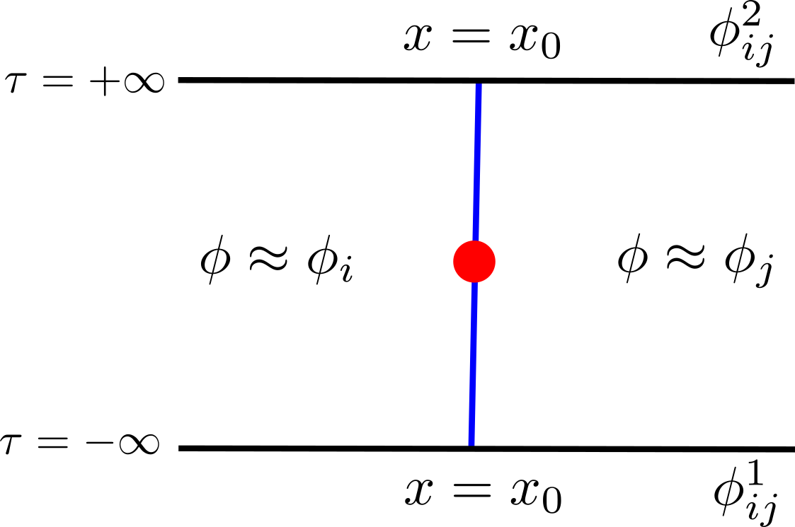
Figure 1: An instanton interpolating between two-different $ij$-solitons

The reason for the failure of the differential $d^{\prime}_{ik}$ (15) is simple, but also interesting: We have missed instantons.

The spaces $R_{ij}$ are made of perturbative BPS states $|\phi_{ij}\rangle$ coming from quantizing around a classical soliton $\phi_{ij}$. The differentials $d_{ij}$ on $R_{ij}$ are meant to encode matrix elements

$$\displaystyle\langle\phi^{b}_{ij}|\mathcal{Q}_{ij}|\phi^{a}_{ij}\rangle,$$ (25)

where the superscripts $a,b$ label different classical solitons of type $ij$. When these are non-zero there is a difference between the exact ground states and the perturbative ones. We know from the relation between Morse theory and supersymmetry [Wit2], that the former are computed by considering suitable instantons between these perturbative ground states. Now within a fixed sector, say the $ij$-sector, solutions of such an instanton on the plane look as in Figure 1: The soliton $\phi_{ij}^{a}$ is stationary, sitting at a fixed point $x_{0}$, whereas at an instant $\tau_{0}$, we transition from the $\phi_{ij}^{a}$ to $\phi_{ij}^{b}$. Such a process will contribute to the matrix element if the fermion numbers of $\phi_{ij}^{a}$ and $\phi_{ij}^{b}$ differ by $1$.

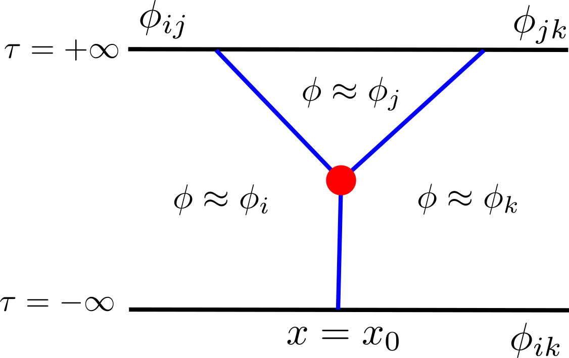
Figure 2: An instanton which contributes to an off-diagonal element of $d^{\prime}_{ik}$.

Close to a wall of marginal stability, it is reasonable to postulate that bound states of $ij$ and $jk$-solitons give rise to an approximate $ik$-soliton, post wall-crossing, thus giving our guess (12). Instantons of the sort depicted in Figure 1, contribute to matrix elements of the type

$$\displaystyle\langle\phi^{b}_{ik}|\mathcal{Q}_{ik}|\phi^{a}_{ik}\rangle$$ (26)

and

$$\displaystyle\langle\phi^{a}_{ij},\phi^{b}_{jk}|\mathcal{Q}_{ik}|\phi^{a^{\prime}}_{ij},\phi^{b^{\prime}}_{jk}\rangle.$$ (27)

Such contributions are indeed reflected in our guess for the differential (15). Our formula for $d^{\prime}_{ik}$ has made an implicit assumption that the off-diagonal matrix element

$$\displaystyle\langle\phi_{ij}^{a},\phi_{jk}^{b}|\mathcal{Q}_{ik}|\phi_{ik}^{c}\rangle$$ (28)

vanishes. However, it turns out, as we will explain in section 3.2 that in addition to the familiar instanton of Figure 1, there can be a more interesting object, where a stationary $ik$-soliton can split into $ij$ and $jk$ solitons traveling at just the correct angles to preserve $\mathcal{Q}_{ik}$-supersymmetry. Such an instanton is depicted in Figure 2. Counting instantons of this type allows one to write down a corrected differential on $R^{\prime}_{ik}$. This is the main new ingredient that enters the categorified wall-crossing formula.

1.3 Wall-Crossing Invariants

In order to derive wall-crossing formulas such as (6) it is extremely useful to introduce certain wall-crossing invariants. For Cecotti-Vafa wall-crossing an example of such a wall-crossing invariant is the spectrum generator

$$\displaystyle S=\prod^{\text{\Large$\curvearrowright$}}_{Z_{ij}\in\mathbb{H}}(\mathbf{1}+\mu_{ij}e_{ij})\in SL(|\mathbb{V}|,\mathbb{Z})$$ (29)

which must be invariant under crossing marginal stability walls [KoSo1], so long as no BPS rays enter of exit the half-plane $\mathbb{H}$. The wall-crossing invariant $S$ has a simple conceptual meaning. One can show that $S_{ij}$ is the Witten index of the space of boundary local operators at a junction of thimbles of type $i$ and $j$ [GMW] (a related interpretation appeared in [HIV]), see Figure 3. Such a space is insensitive to marginal stability walls. Nonetheless the BPS indices $S$ at a given point in parameter space allow the computation of the boundary Witten indices $S$. Comparing $S$ on different sides of the wall of marginal stability leads to (6).

Figure 3: A boundary local operator $\mathcal{O}$ between two branes $L$ and $L^{\prime}$

It is natural then to expect that a categorical wall-crossing invariant can also be constructed. The invariance of $S$ is categorically enhanced as follows. The BPS chain complexes $(R_{ij},d_{ij})$, along with counts of $\zeta$-instantons of the type depicted in Figure 2, allow for the construction of an $A_{\infty}$-category $\widehat{R}[X,W]$ whose objects can be thought of thimble branes and morphisms are vector spaces of boundary local operators at brane junctions [GMW] . The categorical wall-crossing constraint is then formulated as follows.

The homotopy class of $\widehat{R}[X,W]$ is a wall-crossing invariant.

In the above statement homotopy class refers to the homotopy equivalence of $A_{\infty}$-categories which is defined in Appendix B. We show how our categorical wall-crossing formula can be derived from this wall-crossing constraint in section 6.

Remark

Note that instead of $\widehat{R}[X,W]$, there are other wall-crossing invariants one could have used as a starting point. For instance instead of imposing $A_{\infty}$-equivalence of the “open string algebra” $\widehat{R}[X,W]$ across a marginal stability wall like we do in this paper, one could have imposed $L_{\infty}$-equivalence of the closed string algebra $R_{c}$, defined in [GMW]. Another way of describing the categorical wall-crossing formula makes use of half-BPS interfaces. These can be used to construct a categorical notion of a flat parallel transport on a bundle of categories of boundary conditions over the space of Morse superpotentials [GMW]. The absence of monodromy around contractible cycles that intersect walls of marginal stability implies a categorified version of the invariance of $S$ defined in equation (29). This categorical equation can in turn can be reduced to categorified braid relations. For details see [GMW, M2]. These superficially distinct starting points are all expected to lead to the same eventual result.

1.4 Outline of the Paper

The outline of this paper is as follows. In section 2, we recall the standard discussion of wall-crossing at the level of BPS indices. This is followed in section 3 by a discussion of how to formulate chain complexes that categorify the BPS indices. The crucial concept of a $\zeta$-instanton with fan boundary conditions is discussed and we formulate the statement of categorical wall-crossing by using counts of certain trivalent instantons in section 4. After reviewing the construction of the $A_{\infty}$ category of half-BPS branes associated to a Landau-Ginzburg model in section 5, we show the equivalence of the categorical wall-crossing formula to the homotopy equivalence of $A_{\infty}$ categories constructed on either side of a marginal stability wall in section 6. After a brief digression on fermion degrees of a $\zeta$-instanton in section 7, we turn our attention to some examples that illustrate our formulas in section 8. We conclude with some speculations in section 9 and review some aspects of $A_{\infty}$-theory and homological algebra in Appendices B and A.

2 Wall-Crossing of BPS Indices

While our formulas are expected to hold for arbitrary massive two-dimensional $\mathcal{N}=(2,2)$ theories (with a non-anomalous $U(1)_{R}$-symmetry), it is simplest to work in the setting of Landau-Ginzburg models. A Landau-Ginzburg model is a supersymmetric sigma model with a Kähler manifold target $X$ and a potential of the form

$$\displaystyle V=|dW|^{2},$$ (30)

where $W:X\rightarrow\mathbb{C}$ is a holomorphic function known as the superpotential. More precisely, working in two-dimensional $\mathcal{N}=2$-superspace, we can use the Kähler structure on $X$ to write D-terms

$$\displaystyle L_{D}=\int d^{4}\theta\,K(\Phi,\overline{\Phi}),$$ (31)

and the holomorphicity of $W$ to write F-terms

$$\displaystyle L_{F}=\int d^{2}\theta\,W(\Phi)+\int d^{2}\overline{\theta}\,\overline{W}(\overline{\Phi}),$$ (32)

to get a Lagrangian

$$\displaystyle L=L_{D}+L_{F},$$ (33)

invariant under two-dimensional $\mathcal{N}=(2,2)$ Poincaré supersymmetry. The reader is encouraged to consult [MS1], whose notation we adopt, for more details. Various non-renormalization theorems [Seib] of $W$ tell us that one can get great mileage simply by studying the superpotential and its various properties. One use of the superpotential $W$ is that it is sufficient to study many aspects of BPS states.

Supposing that $W$ only has a finite number of isolated singularities, a familiar argument shows that the classical energy in such a theory obeys the BPS bound,

$$\displaystyle E\geq|Z_{ij}|$$ (34)

where

$$\displaystyle Z_{ij}=W_{i}-W_{j}$$ (35)

and $W_{i}$ denotes the critical value $W(\phi_{i})$ of the critical point $\phi_{i}$. Denoting the bosonic fields of the LG model as $\phi$, the standard Bogomolny trick leads to the BPS equation

$$\displaystyle\frac{d\phi}{dx}=\nabla\text{Re}(\zeta^{-1}W),$$ (36)

known as the $\zeta$-soliton equation, $\zeta$ being an arbitrary phase. Solutions on $\mathbb{R}$ with prescribed vacua $\phi_{i}$ and $\phi_{j}$ at the ends of $\mathbb{R}$ can only exist if

$$\displaystyle\zeta=\zeta_{ji}:=\frac{W_{j}-W_{i}}{|W_{j}-W_{i}|}.$$ (37)

Using intersection theory of vanishing cycles, it is possible to get a well-defined signed count of the number of BPS solitons in the $ij$-sector. Let

$$\displaystyle L_{i}(\zeta) = \{p\in X|\text{lim}_{x\rightarrow-\infty}f^{\zeta}_{x}(p)=\phi_{i}\},$$ (38)

$$R_{i}(\zeta) = \{p\in X|\text{lim}_{x\rightarrow+\infty}f^{\zeta}_{x}(p)=\phi_{i}\}$$ (39)

be the ascending and descending manifolds respectively, emanating from the critical point $\phi_{i}$ of the Morse function $\text{Re}(\zeta^{-1}W)$. $f^{\zeta}_{x}$ denotes the one-parameter map $f^{\zeta}_{x}:X\rightarrow X$ defined by the gradient vector field of $\text{Re}(\zeta^{-1}W)$. We then set

$$\displaystyle\mu_{ij}=L_{i}^{-}\circ R_{j}^{+}$$ (40)

where $L_{i}^{-}=L_{i}(\zeta_{ji}e^{-i\epsilon})$ and $R_{j}^{+}=R_{j}(\zeta_{ji}e^{+i\epsilon})$ and $\epsilon$ is a small positive number. The infinitesimal rotation ensures that the intersection is transversal.

The significance of $\mu_{ij}$ from the perspective of the $\mathcal{N}=2$ field theory defined by $(X,W)$ is that one can show [CFIV, CV1] that

$$\displaystyle\mu_{ij}=\text{Tr}_{\mathcal{H}^{\text{BPS}}_{ij}}(-1)^{F}F$$ (41)

where $F$ is the fermion number and

$$\displaystyle\mathcal{H}_{ij}^{\text{BPS}}=\text{ker}(\mathcal{Q}_{ij})\cap\text{ker}(\overline{\mathcal{Q}}_{ij}),$$ (42)

where

$$\displaystyle\mathcal{Q}_{ij}=Q_{-}-\zeta_{ij}^{-1}\overline{Q}_{+}.$$ (43)

$\mu_{ij}$ is thus a supersymmetry protected index that counts the degeneracy of BPS states of type $ij$. Some of its elementary properties are as follows.

Metric Independence

While the BPS soliton equation does depend on the Kähler metric on $X$, the BPS index $\mu_{ij}$ is metric-independent.

CPT

Reversing $x\rightarrow-x$ takes $F\rightarrow-F$ so that $\mu_{ij}=-\mu_{ji}$.

It is familiar that supersymmetric indices such as the Witten index are quantities that are piecewise constant in parameter space. For instance, we can consider the one-dimensional system given by the real superpotential

$$\displaystyle h=x^{4}+\alpha x^{2}+\beta x.$$ (44)

While the conventional partition function $Z=\text{Tr}(e^{-\beta H})$ of the system will be a very non-trivial function of $\alpha$ and $\beta$, the Witten index $I=\text{Tr}(-1)^{F}e^{-\beta H}$ is simply equal to $+1$,

$$\displaystyle I=1,$$ (45)

irrespective of $\alpha$ and $\beta$. In contrast the behavior of the BPS index is more subtle.

Historically wall-crossing was first noticed by considering points in the parameter space of the Landau-Ginzburg model with

$$\displaystyle W=X^{4}+t_{1}X^{2}+t_{2}X$$ (46)

with distinct symmetry groups. Supposing we start out at $(t_{1},t_{2})=(0,1),$ where the model is $\mathbb{Z}_{3}$-symmetric, the latter permuting the three vacua. We can show that there is indeed a single soliton between each pair of distinct critical points,

$$\displaystyle\mu_{12} = 1,$$ (47)

$$\mu_{23} = 1,$$ (48)

$$\mu_{13} = 1,$$ (49)

a spectrum consistent with the $\mathbb{Z}_{3}$ symmetry. If we move slightly away from this point, the collection of numbers doesn’t change. On the other hand at $(t_{1},t_{2})=(1,0)$, the superpotential has $\mathbb{Z}_{2}$-symmetry. Requiring a $\mathbb{Z}_{2}$-symmetric spectrum requires that one of the solitons disappears and the BPS indices are

$$\displaystyle\mu^{\prime}_{12} = 1,$$ (50)

$$\mu^{\prime}_{23} = 1,$$ (51)

$$\mu^{\prime}_{13} = 0.$$ (52)

Thus BPS indices are examples of indices that are not constant but only piecewise constant.

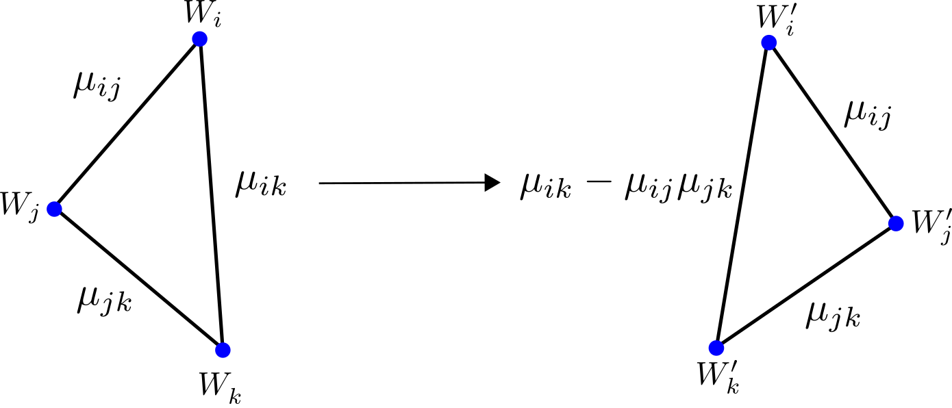
Figure 4: Wall-crossing summarized in the $W$-plane.

The content of the Cecotti-Vafa formula is as follows. It first states that potential discontinuous jumps in the BPS spectrum can occur when three critical values $W_{i},W_{j},W_{k}$ become co-linear as we vary parameters. This is the locus where $\text{Im}(Z_{ij}\overline{Z}_{jk})=0$. Next it gives an explicit formula for the quantitative nature of this jump: If $\mu$ and $\mu^{\prime}$ denote BPS degeneracies on different sides of the wall of marginal stability, they must be related by

$$\displaystyle\mu^{\prime}_{ij} = \mu_{ij},$$ (53)

$$\mu^{\prime}_{jk} = \mu_{jk},$$ (54)

$$\mu^{\prime}_{ik} = \mu_{ik}\pm\mu_{ij}\mu_{jk},$$ (55)

where the sign $-$ is picked in going from the negative side, where $\text{Im}(Z_{ij}\overline{Z}_{jk})<0$ to the positive side, where $\text{Im}(Z_{ij}\overline{Z}_{jk})>0$ and the $+$ is picked in the reverse move. We summarize the formula from the perspective of the $W$-plane in Figure 4.

The trick in arguing for this is to consider not just BPS states, but rather to look at

$$\displaystyle\mathcal{Q}(\zeta)=Q_{-}-\zeta^{-1}\overline{Q}_{+}$$ (56)

preserving boundary conditions of our Landau-Ginzburg model when the latter is formulated on a half-space such as $(-\infty,0]\times\mathbb{R}_{t}$. Such branes have been analyzed in great detail in references, [GMW, HIV]. One finds that the homology class of the support of these branes lives in the finite rank $\mathbb{Z}$-module

$$\displaystyle B(\zeta):=H_{\frac{1}{2}\text{dim}(X)}(X,\text{Re}(\zeta^{-1}W)\rightarrow\infty;\mathbb{Z}).$$ (57)

We can equip $B(\zeta)$ with a natural bilinear form

$$\displaystyle\widehat{\mu}^{\zeta}:B(\zeta)\times B(\zeta)\rightarrow\mathbb{Z},$$ (58)

defined as follows. When $W$ is Morse, there is a natural $\mathbb{Z}$-module basis for $B(\zeta)$ given by the homology class of Lefschetz thimbles $\{[L_{i}(\zeta)]\}_{i\in\mathbb{V}}$. The thimble $L_{i}(\zeta)$ projects to half-infinite rays emanating from the critical value $W_{i}$ in the $\zeta$-direction. We then define

$$\displaystyle\widehat{\mu}^{\zeta}_{ij}:=\widehat{\mu}(L_{i},L_{j})=L^{-}_{i}\circ L^{+}_{j},$$ (59)

where $L^{\pm}$ denote thimbles with phases slightly rotated by a small positive or negative angle respectively, as in Figure 5.

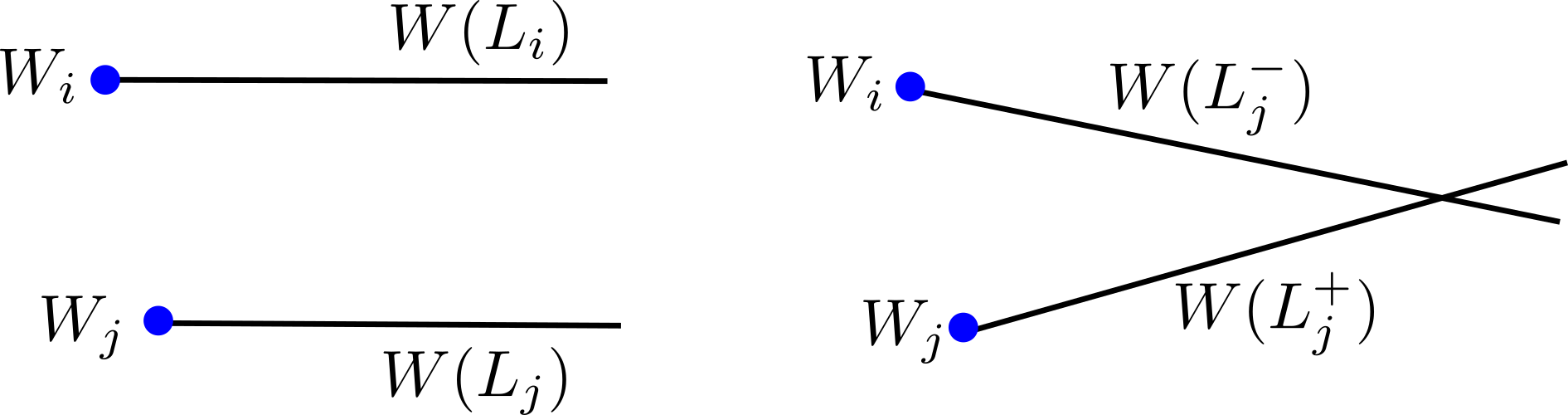
Figure 5: The topological intersection numbers $\widehat{\mu}_{ij}$ obtained by looking at intersection numbers of slightly rotated thimbles.

Some basic properties of $\widehat{\mu}^{\zeta}$ are as follows. First: if $i$ and $j$ are distinct vacua, $\widehat{\mu}^{\zeta}_{ij}$ and $\widehat{\mu}^{\zeta}_{ji}$ cannot both be non-zero. In the case they are equal,

$$\displaystyle\widehat{\mu}_{ii}=1.$$ (60)

Finally, if the vacuum weights are $\zeta$-generic , we can order the thimble basis in decreasing order of $\text{Im}(\zeta^{-1}W_{i})$. Making this choice of ordering, we find that $\widehat{\mu}^{\zeta}$ is an upper-triangular $|\mathbb{V}|\times|\mathbb{V}|$ matrix with $+1$ on the diagonal.

For definiteness and to avoid notational clutter we set $\zeta=1$ and set $\widehat{\mu}=\widehat{\mu}^{\zeta=1}$. This is equivalent to choosing the half-plane in which we take phase ordered products to be the upper-half plane, as was done in (29).

The matrix representation $\widehat{\mu}_{ij}$ for the bilinear form can be calculated from the BPS indices $\mu_{ij}$ by a nice rule expressed in terms of convex geometry.

Definition:

A half-plane fan $F$ of phase $\zeta$ is a collection of vacua $F=\{i_{1},\dots,i_{n}\}$ such that $W(F)=\{W_{i_{1}},\dots,W_{i_{n}}\}$ are the clockwise-ordered vertices of a semi-infinite convex polygon going off to infinity in the $-\zeta$-direction. See Figure 6 for an example with $n=4$. The dual graph looks like a half-plane fan (and indeed has a space-time interpretation), hence the terminology.

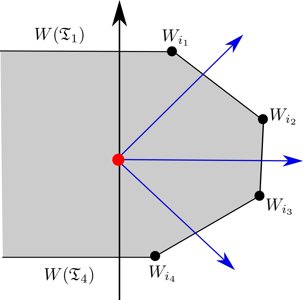
Figure 6: A half-plane fan $F_{i_{1}i_{4}}=\{i_{1},i_{2},i_{3},i_{4}\}$ for $\zeta=1$ and the semi-infinite polygon it forms in the $W$-plane.

To a given half-plane fan $F=\{i_{1},i_{2}.i_{3},\dots,i_{n}\}$ assign the number

$$\displaystyle\mu_{F}=\mu_{i_{1}i_{2}}\mu_{i_{2}i_{3}}\dots\mu_{i_{n-1}i_{n}}.$$ (61)

We then make the

Claim

$$\displaystyle\widehat{\mu}_{ij}=\sum_{\begin{subarray}{c}F_{ij}=\{i,i_{1},\dots,i_{k},j\}\\ F_{ij}\text{ half-plane fan}\end{subarray}}\mu_{ii_{1}}\dots\mu_{i_{k}j}.$$ (62)

Proof

The proof is a straightforward inductive argument, where we induct on distance between $i$ and $j$. To show the base case, for two neighboring vacua $i<j$, one has $\widehat{\mu}_{ij}=\mu_{ij}$ due to (40). On the other hand there’s only one polygon between two neighboring vacua, whose finite segment is given by the segment connecting them, to which we also assign $\mu_{ij}$. For the inductive step, assume that the polygon rule (62) holds for vacua that are up to $n$ units apart and consider a pair of vacua $\{i,j\}$ that are $n+1$ units apart. We know that

$$\displaystyle L_{i}\circ\widetilde{L}_{j}=\mu_{ij}$$ (63)

where $\widetilde{L}_{j}:=L_{j}(\zeta_{ij}e^{-i\epsilon})$. We thus want to compare $\widetilde{L}_{j}$ with $L_{j}^{+}$ namely we must rotate this thimble in a clockwise direction by the phase of $\zeta_{ij}$. In doing this rotation we pick up Picard-Lefschetz discontinuities: For each critical value $W_{k}$ such that $\{i,k,j\}$ forms half-plane fan, we pick up a contribution of $L^{+}_{k}\mu_{ki}$. Summing these up we get

$$\displaystyle L^{+}_{j}=\widetilde{L}_{j}+\sum_{\begin{subarray}{c}k\\ \{i,k,j\}\text{ is a fan}\end{subarray}}L^{+}_{k}\mu_{ki}.$$ (64)

Thus we can compute that

$$\displaystyle\widehat{\mu}_{ij}=\mu_{ij}+\sum_{\begin{subarray}{c}k\text{ s.t.}\\ \{i,k,j\}\text{ is a fan}\end{subarray}}\widehat{\mu}_{ik}\mu_{kj}.$$ (65)

The polygon rule applies to $\widehat{\mu}_{ik}$ so that

$$\displaystyle\widehat{\mu}_{ik}\mu_{kj}=\sum_{F_{ik}}\mu_{F_{ik}}\mu_{kj}.$$ (66)

On the other hand if $\{i,k,j\}$ is a fan, we can form an $ij$ half-plane fan by taking the fan $F_{ik}=\{i,\dots,k\}$ and putting $j$ at the end $\{i,\dots,k,j\}$. To this one precisely assigns $\mu_{F_{ik}}\mu_{kj}$. Conversely, every $ij$ fan can be obtained in this way. ∎

To see that this implies the wall-crossing formula, consider $\widehat{\mu}$ restricted to the three-dimensional $\{i,j,k\}$ space and note that if we are on the left side of Figure 4 then there is only one half-plane of type $ij$ $ik$ $jk$ respectively, so that

$$\displaystyle\widehat{\mu}=\begin{pmatrix}1&&\mu_{ij}&&\mu_{ik}\\ 0&&1&&\mu_{jk}\\ 0&&0&&1\end{pmatrix}.$$ (67)

On the other side of the wall we have two half-plane fans of type $ik$, depicted in Figure 10, leading us to write

$$\displaystyle\widehat{\mu}=\begin{pmatrix}1&&\mu^{\prime}_{ij}&&\mu^{\prime}_{ik}+\mu^{\prime}_{ij}\mu^{\prime}_{jk}\\ 0&&1&&\mu^{\prime}_{jk}\\ 0&&0&&1\end{pmatrix}.$$ (68)

The two expressions for $\widehat{\mu}$ are equal if and only if the wall-crossing formula holds.

More generally suppose that $\{l,m\}$ is any pair of vacua such that there is a fan

$$\displaystyle F_{lm}=\{l,i_{1},\dots,i,k,\dots,i_{n},m\}$$ (69)

in which $\{i,k\}$ appears as a subset of consecutive vacua. Then on the other side of the wall, for every such fan, the set of $lm$-fans gains an additional fan obtained by taking $F_{lm}$ and inserting $j$ in between $i$ and $k$. Moreover these are the only additional fans we gain, assuming we cross no other marginal stability walls in the move. Thus we compare

$$\displaystyle\mu_{li_{1}}\dots\mu_{ik}\dots\mu_{i_{n}m}$$ (70)

with

$$\displaystyle\mu_{li_{1}}\dots\mu^{\prime}_{ik}\dots\mu_{i_{n}m}+\mu_{li_{1}}\dots\mu^{\prime}_{ij}\mu^{\prime}_{jk}\dots\mu_{i_{n}m}$$ (71)

and the two are equal if and only if the wall-crossing formula holds. Therefore we conclude that the wall-crossing formula is equivalent to the invariance of the bilinear form $\widehat{\mu}$ across a wall of marginal stability.

3 BPS Chain Complexes and $\zeta$-instantons

3.1 BPS Chain Complexes

The chain complexes $R_{ij}$ that categorify $\mu_{ij}$ can be formulated by using an infinite-dimensional version of Morse theory. Suppose that the symplectic form $\omega$ on $X$ is exact and choose a Liouville form $\lambda$ so that $\omega=d\lambda$. We consider the (family of) “Morse” functions

$$\displaystyle h_{\zeta}[\phi]=\int_{\mathbb{R}}\phi^{*}(\lambda)+\text{Im}\big{(}\zeta^{-1}W(\phi)\big{)}dx$$ (72)

acting on the space

$$\displaystyle\mathscr{X}_{ij}=\{\phi:\mathbb{R}\rightarrow X|\text{lim}_{x\rightarrow-\infty}\phi(x)=\phi_{i}\,\,\,\,\text{lim}_{x\rightarrow\infty}\phi(x)=\phi_{j}\}.$$ (73)

Generators

The critical points are the points where $\delta h_{\zeta}=0$ which are solutions of the $\zeta$-soliton equation

$$\displaystyle\frac{d\phi^{I}}{dx}=\frac{\zeta}{2}g^{I\bar{J}}\frac{\partial\overline{W}}{\partial\overline{\phi}^{\bar{J}}},$$ (74)

and so the critical point set is non-empty only for $\zeta=\zeta_{ji}$. The Morse function is actually not Morse because of the translational invariance of the soliton equation but we can mod out the solution space by this $\mathbb{R}$-action to obtain a (generically) finite set of critical points, in one-to-one correspondence with intersection points

$$\displaystyle L_{i}(\zeta_{ji}e^{-i\epsilon})\cap R_{j}(\zeta_{ji}e^{i\epsilon}).$$ (75)

Thus we look to the pair

$$\displaystyle(\mathscr{X}_{ij},h_{-\zeta_{ij}})$$ (76)

and assign a $\mathbb{Z}$-module $R_{ij}$ with one generator for each solution of the $\zeta_{ji}$-soliton equation

$$\displaystyle R_{ij}=\bigoplus_{p\in L_{i}^{-}\cap R_{j}^{+}}\mathbb{Z}\langle\phi_{ij}^{p}\rangle.$$ (77)

Gradations

Next we come to the subtle business of defining gradations on $R_{ij}$. The Fermion number, or homological degree of a generator in the Morse complex for a Morse function $f$ as reviewed in [GMW, MS1] is given by

$$\displaystyle-\frac{1}{2}\sum_{\lambda\in\text{Spec }\text{Hess}(f(p))}\text{sign}(\lambda),$$ (78)

where $p$ is the critical point of $f$ whose degree we’re computing. To assign a degree to a $\zeta$-soliton we must therefore compute the second derivative $\delta^{2}h_{\zeta}$. Equivalently we may linearize the $\zeta$-soliton equation (74) which leads to

$$\displaystyle D^{(1,0)}_{x}\delta\phi^{I}=\frac{\zeta}{2}g^{I\bar{J}}D_{\bar{J}}\partial_{\bar{K}}\overline{W}\delta\overline{\phi}^{\bar{K}}$$ (79)

where

$$\displaystyle D^{(1,0)}_{x}\delta\phi^{I}=\frac{\partial}{\partial x}\delta\phi^{I}+\Gamma^{I}_{JK}\frac{\partial\phi^{J}}{\partial x}\delta\phi^{K}$$ (80)

is the pullback connection on $\phi^{*}(T^{(1,0)}X)$. By considering also the complex conjugate of (79), we can write the linearized soliton equation as

$$\displaystyle D_{\zeta}\delta\phi=0$$ (81)

where $D_{\zeta}$ is a Dirac type operator

$$\displaystyle D_{\zeta}:\Gamma\big{(}\phi^{*}(T^{(1,0)}X)\oplus\phi^{*}(T^{(0,1)}X)\big{)}\rightarrow\Gamma\big{(}\phi^{*}(T^{(1,0)}X)\oplus\phi^{*}(T^{(0,1)}X)\big{)}.$$ (82)

Writing

$$\displaystyle\delta\phi\in\Gamma\big{(}\phi^{*}(T^{(1,0)}X)\oplus\phi^{*}(T^{(0,1)}X)\big{)}$$ (83)

as a column vector

$$\displaystyle\delta\phi=\begin{pmatrix}\delta\phi^{I}\\ \delta\overline{\phi}^{\bar{I}}\end{pmatrix}$$ (84)

the operator $D_{\zeta}$ reads

$$\displaystyle\begin{split}D_{\zeta}=\begin{pmatrix}\delta^{I}_{J}\partial_{x}+\Gamma^{I}_{JK}\partial_{x}\phi^{K}&&0\\ 0&&\delta^{\bar{I}}_{\bar{J}}\partial_{x}+\Gamma^{\bar{I}}_{\bar{J}\bar{K}}\partial_{x}\overline{\phi}^{\bar{K}}\end{pmatrix}\,\,\,\,\,\,\,\,\,\,\,\,\,\,\,\,\,\,\,\,\,\,\,\,\,\,\,\,\,\,\,\,\,\,\,\,\,\,\,\,\,\,\,\,\,\,\,\,\\ -\begin{pmatrix}0&&\frac{\zeta}{2}g^{I\bar{K}}D_{\bar{K}}\partial_{\bar{J}}\overline{W}\\ \frac{\zeta^{-1}}{2}g^{\bar{I}K}D_{K}\partial_{J}W&&0\end{pmatrix}.\end{split}$$ (85)

The operator $D_{\zeta}$ is expressed a little more compactly by identifying

$$\displaystyle\phi^{*}(T^{(1,0)}X)\oplus\phi^{*}(T^{(0,1)}X)\cong\phi^{*}(TX),$$ (86)

where $TX$ denotes the complexified tangent bundle. Choosing real coordinates indexed by $a=1,\dots,\text{dim}_{\mathbb{R}}(X)$, we can write

$$\displaystyle D_{\zeta}=\delta^{a}_{b}D_{x}-g^{ac}D_{b}\partial_{c}\,\text{Re}(\zeta^{-1}W),$$ (87)

where

$$\displaystyle D_{x}\delta\phi^{a}=\partial_{x}\delta\phi^{a}+\Gamma^{a}_{bc}\partial_{x}\phi^{b}\,\delta\phi^{c}$$ (88)

is now the pullback connection on $\phi^{*}(TX)$. The Fermion number of an $ij$-soliton $\phi$ should thus be given by a regularized version of (78):

$$\displaystyle F(\phi) = -\text{lim}_{\epsilon\rightarrow 0}\frac{1}{2}\sum_{\lambda\in\text{Eigenvalues}(D_{\zeta_{ji}}(\phi))}\text{sign}(\lambda)e^{-\epsilon|\lambda|}$$ (89)

$$= -\frac{1}{2}\eta\big{(}D_{\zeta_{ij}}(\phi)\big{)}.$$ (90)

One wants chain complexes $R^{(1)}_{ij},R^{(2)}_{ij}$ constructed from two different choices of Kähler metrics $g^{(1)},g^{(2)}$ (namely by a different choice of D-terms) to be homotopy equivalent

$$\displaystyle R^{(1)}_{ij}\simeq R^{(2)}_{ij}.$$ (91)

A necessary condition for is this that if we continuously interpolate between the metrics $g^{(1)}$ and $g^{(2)}$ and evolve the soliton $\phi^{(1)}$ solving the $\zeta$-soliton equation for $g^{(1)}$ to $\phi^{(2)}$ a soliton for $g^{(2)}$ then their Fermion degrees must match. However the variational formula for the $\eta$-invariant says that

$$\displaystyle\frac{1}{2}\eta\big{(}D(\phi^{(1)},g^{(1)})\big{)}-\frac{1}{2}\eta\big{(}D(\phi^{(2)},g^{(2)})\big{)}=2\int_{\mathbb{R}\times[0,1]}\widetilde{\phi}^{*}\Big{(}\frac{1}{2\pi}\text{Tr}\,\mathcal{R}\Big{)},$$ (92)

where

$$\displaystyle\widetilde{\phi}:\mathbb{R}\times[0,1]\rightarrow X$$ (93)

is a path in $\mathscr{X}_{ij}$ interpolating between $\phi^{(1)}$ and $\phi^{(2)}$, and

$$\displaystyle\frac{1}{2\pi}\text{Tr}\,\mathcal{R}$$ (94)

is the Chern-Weil representative of $c_{1}(TX)$. This is nothing but a reminder that the LG model has an axial anomaly for arbitrary Kähler target. The axial anomaly is traditionally expressed as the statement that the right hand side of (92) measures the net violation of Fermion number. The factor of two comes from taking into account the individual violations of both left and right moving fermions. Thus gradations are unchanged under metric variations only if $X$ is Calabi-Yau. Otherwise to ensure this property we must grade $R_{ij}$ by a cyclic group $\mathbb{Z}_{N}$ such that the image of $2c_{1}(X)$ in $H^{2}(X,\mathbb{Z}_{N})$ vanishes.

Differential

The differential $d_{ij}$ is provided by counting (with signs) solutions of the $\zeta_{ji}$-instanton equation

$$\displaystyle\partial_{\overline{s}}\phi^{I}=\frac{\zeta_{ji}}{2}g^{I\bar{J}}\frac{\partial\overline{W}}{\partial\overline{\phi}^{\bar{J}}}$$ (95)

interpolating between solitons of fermion number differing by a unit. Here $s=x+i\tau$, where $\tau$ is the Euclidean time. Thus we get well-defined chain complexes $(R_{ij},d_{ij})$ from which we can construct $\mathcal{H}^{\text{BPS}}_{ij}$ by taking cohomology

$$\displaystyle\mathcal{H}^{\text{BPS}}_{ij}\cong H^{\bullet}(R_{ij},d_{ij}).$$ (96)

A $\zeta$-instanton which contributes to the differential $d_{ij}$ in spacetime looks like Figure 1. Physically we expect the following properties.

Metric Dependence

BPS chain complexes constructed from two different choices of Kähler metrics should be homotopy equivalent.

CPT

Reversing the spatial coordinate, i.e the path $\phi^{p}_{ij}(-x)$ says that for every basis element $\phi_{ij}^{p}$ of $R_{ij}$ we get an element $\phi_{ji}^{p}$ such that

$$\displaystyle\text{deg}(\phi^{p}_{ji})=1-\text{deg}(\phi_{ij}^{p}).$$ (97)

The shift in degree by $+1$ is a technical consequence of factoring out the translational mode of the soliton. For more details on this point see the discussion in section 12.3 in [GMW]. In basis independent terms, CPT says that we have a degree $-1$ non-degenerate pairing

$$\displaystyle K_{ij}:R_{ij}\otimes R_{ji}\rightarrow\mathbb{Z}.$$ (98)

3.2 $\zeta$-instantons and Interior Amplitudes

As alluded to in the introduction, a categorified wall-crossing formula will involve certain “off-diagonal” maps

$$\displaystyle M[\beta_{ikj}]:R_{ij}\otimes R_{jk}\rightarrow R_{ik}$$ (99)

which allow construction of the correct differential. The construction of this map involves counting $\zeta$-instantons with fan boundary conditions, which we now discuss.

We consider solutions of the $\zeta$-instanton equation

$$\displaystyle\overline{\partial}_{\overline{s}}\phi^{I}=\frac{\zeta}{4}g^{I\bar{J}}\frac{\partial\overline{W}}{\partial\overline{\phi}^{\bar{J}}}$$ (100)

which look like a collection of “boosted solitons” at infinity. See [GMW] sections 14.1-14.2 and Appendix E for more details on such boundary conditions. Let

$$\displaystyle I=\{i_{1},\dots,i_{n}\}$$ (101)

be a cyclic fan of vacua and

$$\displaystyle\boldsymbol{\phi}=\{\phi_{i_{1}i_{2}},\dots,\phi_{i_{n}i_{1}}\}$$ (102)

be a fan of solitons. We want to consider $\zeta$-instantons which support these particular solitons on the edges. $I$ is a fan if and only if the critical values

$$\displaystyle W_{I}=\{W_{i_{1}},\dots,W_{i_{n}}\}$$ (103)

are the clockwise ordered vertices of a convex polygon in the $W$-plane. Solutions of the $\zeta$-instanton equation with fan boundary conditions are known as a domain-wall junctions and have been studied in [CHT, GT, INOS], and elsewhere. In particular, it was noted in [CHT], that just the way a $\zeta_{ij}$-soliton maps to a line connecting $W_{i}$ and $W_{j}$ in the $W$-plane, a $\zeta$-instanton maps to the interior of the convex polygon with $W_{I}$ as vertices. See Figure 7 for an example with $n=5$. This fact motivates the terminology BPS or gradient polygon for $\boldsymbol{\phi}$, as was introduced in [KKS].

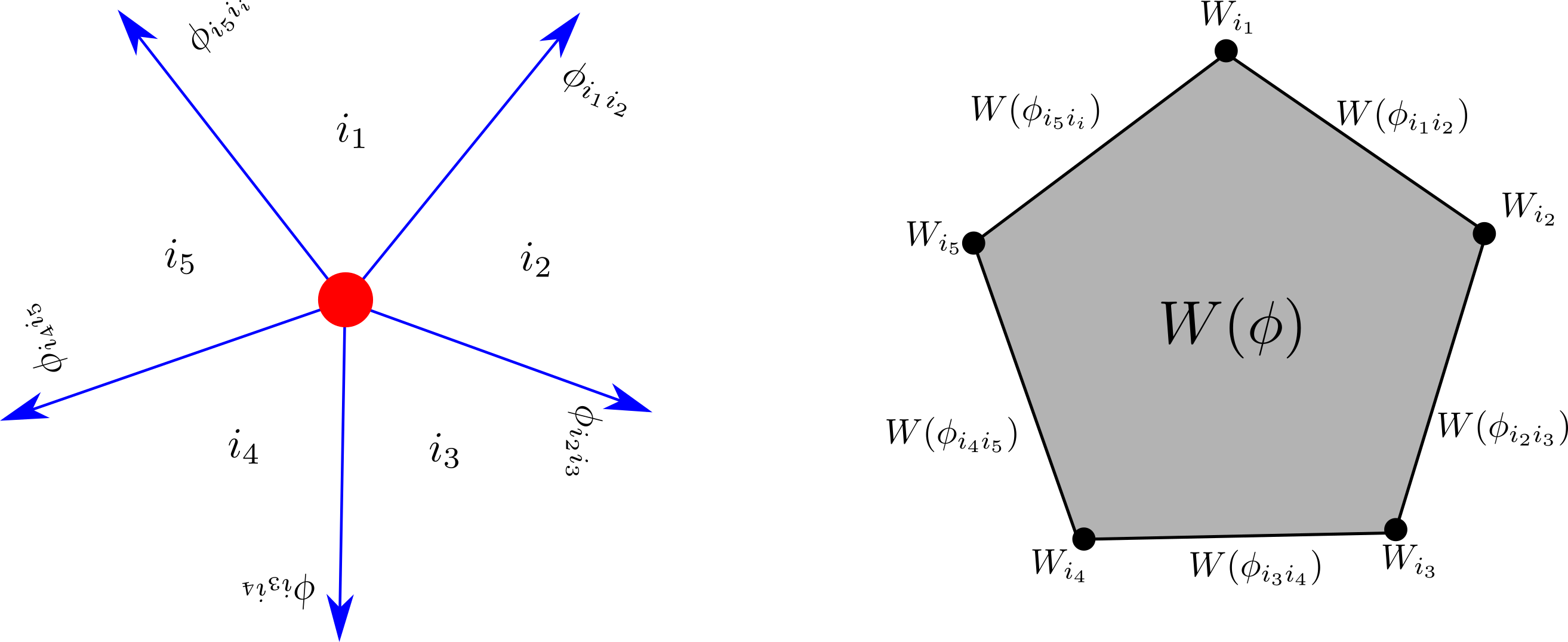
Figure 7: Boundary conditions for a $\zeta$-instanton in the $(x,\tau)$-plane on the left, and the image of such a $\zeta$-instanton in the $W$-plane on the right.

Solutions of the $\zeta$-instanton equation modulo translations with a fixed fan and fixed soliton collection $\boldsymbol{\phi}$ supported on edges form a moduli space $\mathcal{M}_{\zeta}(\boldsymbol{\phi})$. Its dimension is given by forming the vector

$$\displaystyle e_{\boldsymbol{\phi}}:=\phi_{i_{1}i_{2}}\otimes\dots\otimes\phi_{i_{n}i_{1}}$$ (104)

in the cyclic tensor product

$$\displaystyle R_{I}=R_{i_{1}i_{2}}\otimes\dots\otimes R_{i_{n}i_{1}}$$ (105)

and considering its degree

$$\displaystyle F(\boldsymbol{\phi}):=\text{deg}(e_{\boldsymbol{\phi}}).$$ (106)

The (virtual) dimension of these moduli spaces is [GMW]

$$\displaystyle\text{dim}(\mathcal{M}_{\zeta}(\boldsymbol{\phi}))=F(\boldsymbol{\phi})-2.$$ (107)

Moreover $\mathcal{M}_{\zeta}(\boldsymbol{\phi})$ can be oriented. In particular if $F({\boldsymbol{\phi}})=2$, we learn that the moduli space $\mathcal{M}_{\zeta}(\boldsymbol{\phi})$ is a collection of oriented points and thus we can get a well-defined signed count of $\zeta$-instantons

$$\displaystyle N_{\zeta}(\boldsymbol{\phi}):=\#\mathcal{M}_{\zeta}(\boldsymbol{\phi}).$$ (108)

The integers $N(\boldsymbol{\phi})$ satisfy some miraculous identities . There is an identity corresponding to each cyclic fan.

For a cyclic fan of length two, $\{i,j\}$ we have

$$\displaystyle\sum_{\begin{subarray}{c}\chi_{ij}\in L_{i}^{-}\cap R_{j}^{+}\\ F(\phi_{ij},\chi_{ji})=2\\ F(\chi_{ij},\psi_{ji})=2\end{subarray}}N\big{(}\phi_{ij},\chi_{ji}\big{)}N\big{(}\chi_{ij},\psi_{ji}\big{)}=0.$$ (109)

This is nothing but the identity that the differential $d_{ij}$ counting $\zeta$-instantons between $ij$-solitons is nilpotent, which is a familiar fact from Morse theory. It involves the fact that the moduli space $\mathcal{M}(\phi_{ij},\psi_{ji})$ such that $d(\phi_{ij},\psi_{ji})=3$ has ends corresponding to broken flow lines gluing intermediate instantons.

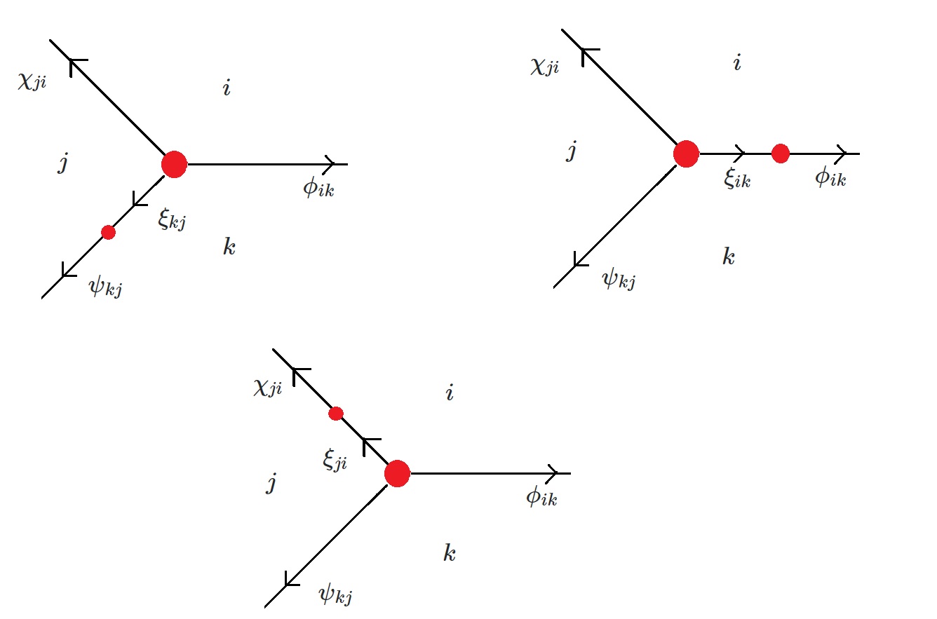
Figure 8: The various ends of $\mathcal{M}\big{(}\phi_{ik},\psi_{kj},\chi_{ji})$ where $F(\phi_{ik},\psi_{kj},\chi_{ji})=3.$

For $\{i,k,j\}$ a cyclic fan of vacua of length three, we have the identity

$$\displaystyle\begin{split}\sum_{\begin{subarray}{c}\xi_{ij}\in L_{i}^{-}\cap R_{j}^{+}\\ F(\phi_{ik},\psi_{kj},\xi_{ji})=2\\ F(\xi_{ij},\chi_{ji})=2\end{subarray}}N(\phi_{ik},\psi_{kj},\xi_{ji}\big{)}N\big{(}\xi_{ij},\chi_{ji}\big{)}\\ +\sum_{\begin{subarray}{c}\xi_{jk}\in L_{j}^{-}\cap R_{k}^{+}\\ F(\chi_{ji},\phi_{ik},\xi_{kj})=2\\ F(\xi_{jk},\psi_{kj})=2\end{subarray}}N\big{(}\chi_{ji},\phi_{ik},\xi_{kj}\big{)}N\big{(}\xi_{jk},\psi_{kj}\big{)}\\ +\sum_{\begin{subarray}{c}\xi_{ik}\in L_{i}^{-}\cap R_{k}^{+}\\ F(\xi_{ik},\psi_{kj},\chi_{ji})=2\\ F(\phi_{ik},\xi_{ki})=2\end{subarray}}N\big{(}\phi_{ik},\xi_{ki}\big{)}N\big{(}\xi_{ik},\psi_{kj},\chi_{ji}\big{)}=0.\end{split}$$ (110)

The argument for this involves looking at the ends of the moduli space

$$\displaystyle\mathcal{M}\big{(}\phi_{ik},\psi_{kj},\chi_{ji})$$ (111)

of a fan of solitons such that $F(\phi_{ik},\psi_{kj},\chi_{ji})=3.$ There are three types of ends, where a rigid instanton of type $\{i,k\}$ is glued to a rigid instanton of type $\{i,k,j\}$, similarly for $\{i,j\}$ and $\{j,k\}$. See Figure 8. Such “broken flows” give

$$\displaystyle\begin{split}\partial\mathcal{M}\big{(}\phi_{ik},\psi_{kj},\chi_{ji})=\bigsqcup_{\begin{subarray}{c}\xi_{ij}\in L_{i}^{-}\cap R_{j}^{+}\\ F(\phi_{ik},\psi_{kj},\xi_{ji})=2\\ F(\xi_{ij},\chi_{ji})=2\end{subarray}}\mathcal{M}\big{(}\phi_{ik},\psi_{kj},\xi_{ji}\big{)}\times\mathcal{M}\big{(}\xi_{ij},\chi_{ji}\big{)}\\ \sqcup\bigsqcup_{\begin{subarray}{c}\xi_{jk}\in L_{j}^{-}\cap R_{k}^{+}\\ F(\chi_{ji},\phi_{ik},\xi_{kj})=2\\ F(\xi_{jk},\psi_{kj})=2\end{subarray}}\mathcal{M}\big{(}\chi_{ji},\phi_{ik},\xi_{kj}\big{)}\times\mathcal{M}\big{(}\xi_{jk},\psi_{kj}\big{)}\\ \sqcup\bigsqcup_{\begin{subarray}{c}\xi_{ik}\in L_{i}^{-}\cap R_{k}^{+}\\ F(\xi_{ik},\psi_{kj},\chi_{ji})=2\\ F(\phi_{ik},\xi_{ki})=2\end{subarray}}\mathcal{M}\big{(}\phi_{ik},\xi_{ki}\big{)}\times\mathcal{M}\big{(}\xi_{ik},\psi_{kj},\chi_{ji}\big{)}.\end{split}$$ (112)

(110) then follows from

$$\displaystyle\#\partial\mathcal{M}\big{(}\phi_{ik},\psi_{kj},\chi_{ji})=0.$$ (113)

More generally, one expects that the moduli spaces $\mathcal{M}_{\zeta}(\boldsymbol{\phi})$ can be compactified, such that the compactified moduli space $\overline{\mathcal{M}}_{\zeta}(\boldsymbol{\phi})$ has strata labeled by web diagrams of the type in Figure 8.

Although the identities (109) and (110) are all we need for categorical wall-crossing, we should mention for completeness that there are more complicated identities involving fans of longer length which can be deduced from the web combinatorics of [GMW]. The summary is that all identities follow from a single $L_{\infty}$-Maurer-Cartan equation. Form the vector space

$$\displaystyle R_{c} = \oplus_{I}R_{I}$$ (114)

$$= \oplus_{i\in\mathbb{V}}R_{i}\oplus_{i\neq j}(R_{ij}\otimes R_{ji})\oplus\dots$$ (115)

corresponding to taking all possible cyclic tensor products. $R_{c}$ has the structure of an $L_{\infty}$-algebra. Namely there are maps

$$\displaystyle\rho(\mathfrak{t}):S_{+}R_{c}\rightarrow R_{c},$$ (116)

where $S_{+}R_{c}$ denotes (the positive part of) the symmetric algebra, satisfying $L_{\infty}$-axioms. $\rho(\mathfrak{t})$ is defined through taut webs as in [GMW]. Define

$$\displaystyle\beta_{I}:=\sum_{\begin{subarray}{c}\boldsymbol{\phi}\text{ gradient polygons for }I\\ F(\boldsymbol{\phi})=2\end{subarray}}N(\boldsymbol{\phi})e_{\boldsymbol{\phi}},$$ (117)

and let

$$\displaystyle\beta:=\sum_{I}\beta_{I}\in R_{c}.$$ (118)

One of the main results of [GMW] is that analysis of various moduli spaces leads one to conclude that $\beta$ is a Maurer-Cartan element for the $L_{\infty}$-structure. Namely it satisfies the $L_{\infty}$ Maurer-Cartan equation

$$\displaystyle\rho(\mathfrak{t})(e^{\beta})=0.$$ (119)

$\beta$ was called the interior amplitude in [GMW]. The identities (109), (110) are some simple equations that come from unpacking the $L_{\infty}$ Maurer-Cartan equation.

Remark

In general interior amplitudes will have components associated to arbitrary fans

$$\displaystyle\beta_{i_{1}i_{2}\dots i_{n}}\in R_{i_{1}i_{2}}\otimes R_{i_{2}i_{3}}\otimes\dots\otimes R_{i_{n}i_{1}}.$$ (120)

However, only the trivalent components associated to the “wall-crossing triangle”; $\beta_{ikj}$ on one side and $\beta^{\prime}_{ijk}$ on the other, enter the discussion in categorical wall-crossing.

3.3 Homotopy Equivalence of BPS Data

We have discussed the construction of the BPS chain complexes

$$\displaystyle\{(R_{ij},d_{ij})\},$$ (121)

the contraction maps

$$\displaystyle\{K_{ij}\}$$ (122)

and the important vector encoding counts of rigid $\zeta$-instantons

$$\displaystyle\beta\in R_{c}.$$ (123)

We have noted however that the BPS complexes by themselves are not physical observables, only their homotopy equivalence class is. It is natural to try to extend the notion of homotopy equivalence from the BPS complexes, to the full categorical BPS data, namely to introduce a natural notion of homotopy equivalence for the contraction pairings and interior amplitudes. We briefly formulate such a notion in this sub-section.

Suppose we are given another collection of BPS data $(\{S_{ij}\},\{L_{ij}\},\gamma)$ where $S_{ij}$ denote complexes $L_{ij}$ contaction maps, and $\gamma$ is now a Maurer-Cartan element of the $L_{\infty}$-algebra $S_{c}$, constructed from $S_{ij}$ and $L_{ij}$. We say that the BPS data

$$\displaystyle\big{(}\{R_{ij}\},\{K_{ij}\},\beta\big{)}\text{ and }\big{(}\{S_{ij}\},\{L_{ij}\},\gamma)$$ (124)

are homotopy equivalent if there are homotopy equivalences of chain complexes

$$\displaystyle f_{ij}:R_{ij}\rightarrow S_{ij}$$ (125)

that fit into a collection of maps

$$\displaystyle f_{n}:R_{c}^{\otimes n}\rightarrow S_{c}$$ (126)

with $f_{1}$ being induced canonically from the collection $\{f_{ij}\}$ that together define an $L_{\infty}$-equivalence from $R_{c}$ to $S_{c}$. The maps $\{f_{ij}\}$ and the $L_{\infty}$-morphism $\{f_{n}\}$ must be such that the diagram

(131)

commutes up to homotopy, and the Maurer-Cartan element transports naturally:

$$\displaystyle f(e^{\beta})\sim\gamma,$$ (132)

where $\sim$ denotes gauge equivalence of Maurer-Cartan elements, defined in Appendix B.

The general philosophy of this paper is that we should only consider homotopy equivalence classes of the categorical BPS data. For example a D-term variation will only result in homotopy equivalent BPS data. The equivalence in this section can be viewed as a relaxation of the notion of strict isomorphism of categorical BPS data as defined in [GMW] section 4.1.1.

4 Statement of Categorical Wall-Crossing

Notation

Given an element $r_{ik}\otimes r_{kj}\otimes r_{ji}\in R_{ik}\otimes R_{kj}\otimes R_{ji}$ we can define

$$\displaystyle M[r_{ik}\otimes r_{kj}\otimes r_{ji}]:R_{ij}\otimes R_{jk}\rightarrow R_{ik}$$ (133)

by using the contraction maps

$$\displaystyle M[r_{ik}\otimes r_{kj}\otimes r_{ji}](r^{\prime}_{ij}\otimes r^{\prime}_{jk})=K_{ji}(r_{ji},r^{\prime}_{ij})K_{kj}(r_{kj},r^{\prime}_{jk})r_{ik}.$$ (134)

Similarly we define

$$\displaystyle M^{\prime}[r_{ik}\otimes r_{kj}\otimes r_{ji}]:R_{ki}\rightarrow R_{kj}\otimes R_{ji}$$ (135)

by contracting the $ik$ factor using $K_{ik}$, and using the Koszul sign rule. Finally the natural product rule differential on a tensor product chain complex of the form as $R_{ij}\otimes R_{jk}$ is denoted as $d_{ijk}$:

$$\displaystyle d_{ijk}=d_{ij}\otimes 1\pm 1\otimes d_{jk}.$$ (136)

When we write $\pm$ it means we are not being precise about the exact sign.

Marginal Stability Wall

Recall an $ijk$ wall of marginal stability is the locus where

$$\displaystyle\text{Im}(Z_{ij}\overline{Z}_{jk})=0.$$ (137)

See Figure 9.

Main Statement

Let

$$\displaystyle(R_{ij},R_{jk},R_{ik},\beta_{ikj})$$ (138)

be the chain complexes and interior amplitude component in a region where

$$\displaystyle\text{Im}(Z_{ij}\overline{Z}_{jk})<0,$$ (139)

and

$$\displaystyle(R^{\prime}_{ij},R^{\prime}_{jk},R^{\prime}_{ik},\beta^{\prime}_{ijk})$$ (140)

be the chain complexes and interior amplitude component in a region where

$$\displaystyle\text{Im}(Z^{\prime}_{ij}\overline{Z}^{\prime}_{jk})>0.$$ (141)

Note that $\beta_{ikj}$ defines a chain map

$$\displaystyle M[\beta_{ikj}]:R_{ij}\otimes R_{jk}\rightarrow R_{ik},$$ (142)

and $\beta^{\prime}_{ijk}$ defines a chain map

$$\displaystyle M^{\prime}[\beta^{\prime}_{ijk}]:R^{\prime}_{ik}[1]\rightarrow R^{\prime}_{ij}\otimes R^{\prime}_{jk}.$$ (143)

The categorical wall-crossing formula states that

$$\displaystyle R^{\prime}_{ij} \simeq R_{ij},$$ (144)

$$R^{\prime}_{jk} \simeq R_{jk},$$ (145)

$$R^{\prime}_{ik} \simeq \text{Cone}\big{(}M[\beta_{ikj}]:R_{ij}\otimes R_{jk}\rightarrow R_{ik}\big{)}.$$ (146)

Furthermore, letting $(P,Q)$ be the chain maps that implement the homotopy equivalence between the primed and unprimed sides, it states that the diagrams

$$\displaystyle\begin{CD}R^{\prime}_{ik}[1]@>{M^{\prime}[\beta^{\prime}_{ijk}]}>{}>R^{\prime}_{ij}\otimes R^{\prime}_{jk}\\ @V{P}V{}V@V{}V{P\otimes P}V\\ \text{Cone}\big{(}M[\beta_{ikj}]\big{)}[1]@>{}>{\pi}>R_{ij}\otimes R_{jk}\end{CD}$$ (147)

and

$$\displaystyle\begin{CD}R^{\prime}_{ik}[1]@>{M^{\prime}[\beta^{\prime}_{ijk}]}>{}>R^{\prime}_{ij}\otimes R^{\prime}_{jk}\\ @A{Q}A{}A@A{}A{Q\otimes Q}A\\ \text{Cone}\big{(}M[\beta_{ikj}]\big{)}[1]@>{}>{\pi}>R_{ij}\otimes R_{jk}\end{CD}$$ (148)

commute up to homotopy.

Equivalently,

$$\displaystyle R_{ij} \simeq R^{\prime}_{ij},$$ (149)

$$R_{jk} \simeq R^{\prime}_{jk},$$ (150)

$$R_{ik} \simeq \text{Cone}(M^{\prime}[\beta^{\prime}_{ijk}]:R^{\prime}_{ik}[1]\rightarrow R^{\prime}_{ij}\otimes R^{\prime}_{jk}),$$ (151)

and letting $(S,T)$ be the chain maps implementing homotopy equivalence between the two sides, the diagrams

$$\displaystyle\begin{CD}R_{ij}\otimes R_{jk}@>{M[\beta_{ikj}]}>{}>R_{ik},\\ @V{T\otimes T}V{}V@V{}V{T}V\\ R^{\prime}_{ij}\otimes R^{\prime}_{jk}@>{}>{i}>\text{Cone}\big{(}M^{\prime}[\beta^{\prime}_{ijk}]\big{)}\end{CD}$$ (152)

and

$$\displaystyle\begin{CD}R_{ij}\otimes R_{jk}@>{M[\beta_{ikj}]}>{}>R_{ik},\\ @A{S\otimes S}A{}A@A{}A{S}A\\ R^{\prime}_{ij}\otimes R^{\prime}_{jk}@>{}>{i}>\text{Cone}\big{(}M^{\prime}[\beta^{\prime}_{ijk}]\big{)}\end{CD}$$ (153)

commute up to homotopy.

These formulas are also sufficient to relate the contraction maps. Given chain complexes

$$\displaystyle(R_{ij},R_{jk},R_{ik},\beta_{ikj})$$ (154)

such that

$$\displaystyle\text{Im}(Z_{ij}\overline{Z}_{jk})<0,$$ (155)

the dual complexes $(R_{kj},R_{ji},R_{ki})$ will be a triple such that

$$\displaystyle\text{Im}(Z_{kj}\overline{Z}_{ji})>0.$$ (156)

Therefore the formulas for going from $\text{Im}(\cdots)>0$ to $\text{Im}(\cdots)<0$ imply that

$$\displaystyle R^{\prime}_{kj} \simeq R_{kj},$$ (157)

$$R^{\prime}_{ji} \simeq R_{ji},$$ (158)

$$R^{\prime}_{ki} \simeq \text{Cone}\big{(}M^{\prime}[\beta_{ikj}]:R_{ki}[1]\rightarrow R_{kj}\otimes R_{ji}\big{)}.$$ (159)

Note that there is a canonical degree $-1$ map

$$\displaystyle L:\text{Cone}\big{(}M[\beta_{ikj}]\big{)}\otimes\text{Cone}\big{(}M^{\prime}[\beta_{ijk}])\rightarrow\mathbb{Z}$$ (160)

given by

$$\displaystyle L=\begin{pmatrix}0&&K_{ik}\\ K_{ij}\otimes K_{jk}&&0\end{pmatrix}.$$ (161)

Denote the chain maps implementing the homotopy equivalence as $\widetilde{P},\widetilde{Q}$. With this, the final part of categorical wall-crossing also determines the homotopy class of the contraction maps, by stating that the diagrams

(166)

(171)

(176)

commute up to homotopy. In the above we have abbreviated $\text{Cone}\big{(}M[\beta_{ikj}]\big{)}$ and $\text{Cone}\big{(}M^{\prime}[\beta^{\prime}_{ijk}]\big{)}$ as $\text{C}(M)$ and $\text{C}(M^{\prime})$ respectively. There will be similar diagrams with $(Q,\widetilde{Q})$.

Canonical Representatives

In practice given the chain complexes on one side, one wants to work with specific representatives within the homotopy equivalence class of chain complexes (and chain maps) for the other. There is a canonical choice for this. Suppose we treat the primed side as unknown. Then the canonical representatives for the primed complexes are

$$\displaystyle R^{\prime}_{ij} = R_{ij},$$ (177)

$$R^{\prime}_{jk} = R_{jk},$$ (178)

$$R^{\prime}_{ik} = \text{Cone}\big{(}M[\beta_{ikj}]\big{)}.$$ (179)

By letting $P,Q$ to be identity maps, we can then make the diagrams (147),(148), strictly commute by letting

$$\displaystyle M^{\prime}[\beta^{\prime}_{ijk}]=\pi,$$ (180)

which is equivalent to saying that

$$\displaystyle\beta^{\prime}_{ijk}=K^{-1}_{ij}K^{-1}_{jk}.$$ (181)

The canonical representatives for the dual complexes are

$$\displaystyle R^{\prime}_{kj} = R_{kj},$$ (182)

$$R^{\prime}_{ji} = R_{ji},$$ (183)

$$R^{\prime}_{ki} = \text{Cone}\big{(}M^{\prime}[\beta_{ikj}]\big{)}$$ (184)

and one can then set the contraction maps to be

$$\displaystyle K^{\prime}_{ij} = K_{ij},$$ (185)

$$K^{\prime}_{jk} = K_{jk},$$ (186)

$$K^{\prime}_{ik} = \begin{pmatrix}0&&K_{ik}\\ K_{ij}\otimes K_{jk}&&0\end{pmatrix}.$$ (187)

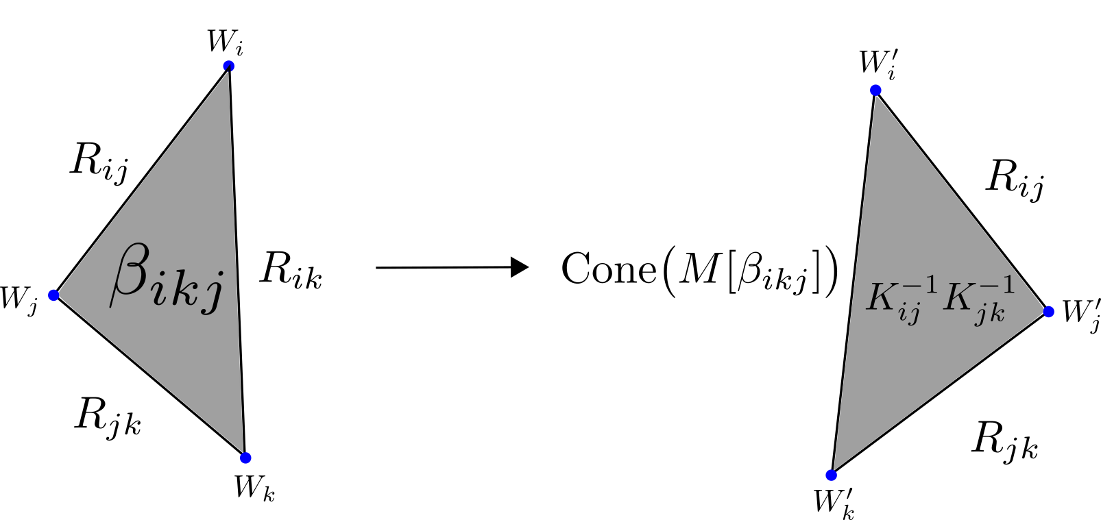
Figure 9: Categorical wall-crossing summarized in the $W$-plane.

Figure 9 summarizes the categorical wall-crossing formula for going from a point in parameter space with $\text{Im}(Z_{ij}\overline{Z}_{jk})<0$ to a point where $\text{Im}(Z_{ij}\overline{Z}_{jk})>0$ from the perspective of the $W$-plane. The formulas and the figure summarizing the specific representatives in the inverse move would look similar. These straightforward details are left for the reader.

Remark: Consistency Check

A consistency check our formulas must pass is whether jumping from the negative side of the wall of marginal stability where $\text{Im}(Z_{ij}\overline{Z}_{jk})<0$ to the positive side where $\text{Im}(Z_{ij}\overline{Z}_{jk})>0$ and then jumping back to the negative side is equivalent to doing nothing. We work with the canonical representatives. Starting from the complex $R_{ik}$ the wall-crossing formula says that

$$\displaystyle R^{\prime}_{ik}=\text{Cone}\big{(}M[\beta_{ijk}]:R_{ij}\otimes R_{jk}\rightarrow R_{ik}\big{)},$$ (188)

and

$$\displaystyle\beta^{\prime}_{ijk}=K_{ij}^{-1}K_{jk}^{-1}.$$ (189)

Jumping back to the right side, gives us

$$\displaystyle R^{\prime\prime}_{ik}=\text{Cone}\big{(}M^{\prime}[K^{-1}_{ij}K^{-1}_{jk}]:\text{Cone}\big{(}M[\beta_{ikj}]\big{)}[1]\rightarrow R_{ij}\otimes R_{jk}\big{)}.$$ (190)

But

$$\displaystyle M^{\prime}[\beta^{\prime}_{ijk}]=\pi$$ (191)

and therefore we have

$$\displaystyle R^{\prime\prime}_{ik} = \text{Cone}\big{(}\pi:\text{Cone}\big{(}M[\beta]:R_{ij}\otimes R_{jk}\rightarrow R_{ik})[1]\rightarrow R_{ij}\otimes R_{jk}\big{)}$$ (192)

$$= \text{Cyl}\big{(}M[\beta_{ikj}]:R_{ij}\otimes R_{jk}\rightarrow R_{ik}\big{)}$$ (193)

$$\simeq R_{ik}.$$ (194)

The cylinder construction of homological algebra, used above is described in Appendix A. Therefore we end up with a complex canonically homotopy equivalent to the original complex. A similar check can be performed for $\beta^{\prime\prime}_{ikj}$. One shows that the diagram

(199)

commutes up to homotopy. This shows clearly the need to work at the level of homotopy equivalence.

In the next two sections we show how these conditions word-for-word are the homotopy equivalence of $A_{\infty}$ categories constructed at a point where $\text{Im}(Z_{ij}\overline{Z}_{jk})>0$ compared to a point where $\text{Im}(Z_{ij}\overline{Z}_{jk})<0$.

5 $\zeta$-instantons and Brane Categories

5.1 Bare Thimble Category

While the chain complex $R_{ij}$ categorifies $\mu_{ij}$, categorification of $\widehat{\mu}_{ij}$ leads to more interesting structure. The correct viewpoint will be that $B$ must be upgraded to a category, and $\widehat{\mu}_{ij}$ will be categorified to vector spaces of morphisms.

The construction of the “bare” thimble category $\widehat{R}^{\text{bare}}$ proceeds as follows.

Objects

The objects are an ordered collection of thimbles

$$\displaystyle\mathfrak{T}_{1},\dots,\mathfrak{T}_{n},$$ (200)

one for each critical point $i\in\text{Crit}(W)$. They are ordered by $\text{Im}(-W)$ so that $i>j$ if $\text{Im}(W_{i})<\text{Im}(W_{j})$.

Morphisms

The morphisms are given as follows. In order to define

$$\displaystyle\widehat{R}_{ij}:=\text{Hop}(\mathfrak{T}_{i},\mathfrak{T}_{j})$$ (201)

we look at all half-plane fans with “top” vacuum $i$ and “bottom” vacuum $j$. To an edge separating $i$ and $j$ assign the vector space $R_{ij}$ and take the (ordered) tensor product along each edge. Thus to each half-plane fan $F_{ij}$ of this type we assign a vector space $R_{F_{ij}}$. The morphism space is then defined by taking direct sums over all $F_{ij}$ half-plane fans

$$\displaystyle\widehat{R}_{ij}=\bigoplus_{F_{ij}}R_{F_{ij}}.$$ (202)

See Figure 10 for an example of a morphism space where two fans contribute. Note that

$$\displaystyle\widehat{R}_{ii}=\text{Hop}(\mathfrak{T}_{i},\mathfrak{T}_{i})=\mathbb{Z}.$$ (203)

If there are no half-plane fans then

$$\displaystyle\widehat{R}_{ij}=0,$$ (204)

so that the objects $\{\mathfrak{T}_{1},\dots,\mathfrak{T}_{n}\}$ are an exceptional collection; the matrix of morphism spaces $\widehat{R}_{ij}$ is an upper-triangular matrix with $\mathbb{Z}$ on the diagonal.

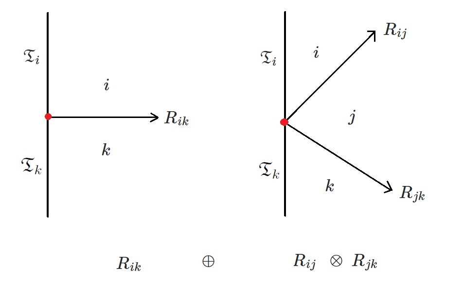
Figure 10: Contribution of some half-plane fans to $\text{Hop}(\mathfrak{T}_{i},\mathfrak{T}_{k})$

Compositions

An associative composition law

$$\displaystyle m_{ijk}:\widehat{R}_{ij}\otimes\widehat{R}_{jk}\rightarrow\widehat{R}_{ik}$$ (205)

is given simply by looking at whether $F_{jk}$ can be placed below $F_{ij}$ to form a fan $F_{ik}$. If so, we take the tensor product of the vectors in $R_{F_{ij}}$ and $R_{F_{jk}}$ to get a vector in $R_{F_{ik}}$. If not, we set it equal to zero.

Differentials

Finally the differential $\widehat{d}_{ij}$ on

$$\displaystyle\widehat{R}_{ij}=R_{ij}\oplus(R_{ik}\otimes R_{kj})\oplus\dots$$ (206)

will be inherited from the differentials on the complexes in the obvious way

$$\displaystyle\widehat{d}_{ij}=d_{ij}\oplus(d_{ik}\otimes 1+1\otimes d_{kj})\oplus\dots.$$ (207)

Remark

The differential-graded algebra

$$\displaystyle\text{End}\big{(}\oplus_{i}\mathfrak{T}_{i})=\bigoplus_{i,j}\widehat{R}_{ij}$$ (208)

in which the algebra multiplication is specified by the morphisms as defined above, as explained in Appendix B, carries the same information as the category $\widehat{R}$ and so we often use the terms algebra and category interchangeably in what follows.

5.2 Interior Amplitudes and Deformations of $\widehat{R}$

While $\widehat{R}^{\text{bare}}$ indeed gives $\widehat{\mu}$ as its matrix of Euler characters, the cohomology space $H^{\bullet}(\widehat{R}_{ij},\widehat{d}_{ij})$ is not very physically meaningful. In particular, it is not isomorphic to the space of boundary BPS local operators at a $\mathfrak{T}_{i}$-$\mathfrak{T}_{j}$ brane junction, like we would want it to be. The reason for this is similar to the failure of our naive categorification: we have not taken into account all $\zeta$-instantons. In particular these $\zeta$-instantons will correct the differential (207) and the composition law (205) described in the previous section.

The precise way to take $\zeta$-instantons into account again uses the interior amplitude $\beta$. Similar to how one can use taut webs with $n$ vertices to define $L_{\infty}$-maps,

$$\displaystyle\rho(\mathfrak{t}^{(n)}):S^{n}R_{c}\rightarrow R_{c},$$ (209)

we can use taut half-plane webs with $p$ boundary vertices and $q$ bulk vertices to define maps

$$\displaystyle\rho(\mathfrak{t}_{\mathcal{H}}^{(p,q)}):(\widehat{R})^{\otimes p}\otimes(R_{c})^{\otimes q}\rightarrow\widehat{R}$$ (210)

which satisfy the $LA_{\infty}$-axioms [GMW] (these are also known as the axioms of an open-closed homotopy algebra, see [KS]). We now make use of the

Theorem

Suppose $(A,L)$ is an open-closed homotopy algebra with structure maps

$$\displaystyle m_{k,l}:A^{\otimes k}\otimes L^{\otimes l}\rightarrow A,\,\,\,\,\,\,k\geq 1,l\geq 0$$ (211)

and suppose $\gamma\in L$ is a Maurer-Cartan element for the $L_{\infty}$ algebra $L$. Then the collection of maps

$$\displaystyle m_{k}[\gamma]:A^{\otimes k}\rightarrow A,$$ (212)

defined by

$$\displaystyle m_{k}[\gamma](-,\dots,-):=\sum_{l\geq 0}\frac{1}{l!}m_{k,l}(-\dots,-,\gamma^{\otimes l})$$ (213)

give a (new) $A_{\infty}$-structure on $A$.

Thus we use the $\zeta$-instanton counting element $\beta$ to deform the dg-category $\widehat{R}^{\text{bare}}$ to an $A_{\infty}$-category denoted by $\widehat{R}[X,W]$. The deformed category $\widehat{R}[X,W]$ is proposed as the physical brane category of the Landau-Ginzburg model associated to the pair $(X,W)$. In particular, we correct the differential $\widehat{d}_{ij}$ to $\widehat{d}_{ij}[\beta]$ via (213) with $k=1$, so that the cohomology

$$\displaystyle H^{\bullet}(\widehat{R}_{ij},\widehat{d}_{ij}[\beta])$$ (214)

is isomorphic to the space of $\frac{1}{2}$-boundary BPS local operators at a $(\mathfrak{T}_{i},\mathfrak{T}_{j})$-brane junction. In addition $k=2$ of (213) also modifies the bilinear composition (205). As a result of (213) higher operations

$$\displaystyle\{m_{k}[\beta]\}_{k>2}$$ (215)

are also introduced. Together these operations turn $\widehat{R}[X,W]$ into a genuine $A_{\infty}$-category.

6 Homotopy Equivalence of Brane Categories

The categorical wall-crossing constraint is formulated as follows.

Categorical Wall-Crossing Constraint

Suppose $W$ and $W^{\prime}$ are superpotentials on different sides of a wall of marginal stability. Then the $\beta$-deformed thimble categories on either side of the wall are homotopy equivalent

$$\displaystyle\widehat{R}[X,W]\simeq\widehat{R}^{\prime}[X,W^{\prime}]$$ (216)

as $A_{\infty}$-categories.

We now relate our categorical wall-crossing formulas with the categorical wall-crossing constraint. First we construct the left and right $\{i,j,k\}$-subcategories. As an instructive first check, we verify that the canonical representatives indeed give homotopy equivalent categories. Finally we unpack the axioms for $A_{\infty}$ equivalence and show how the general statement follows.

6.1 Left Configuration

Let us first construct the $\{i,j,k\}$ sub-algebra of $\widehat{R}$ for the configuration on the left of Figure 4. The soliton complexes are

$$\displaystyle(R_{ij},d_{ij}),(R_{ik},d_{ik}),(R_{jk},d_{jk}).$$ (217)

Because there are no half-plane fans with more than one edge emanating from the boundary, the morphism spaces are simply

$$\displaystyle\widehat{R}_{ij} = R_{ij},$$ (218)

$$\widehat{R}_{jk} = R_{jk},$$ (219)

$$\widehat{R}_{ik} = R_{ik}.$$ (220)

In the undeformed algebra, there are no non-trivial multiplications.

Figure 11: A taut half-plane web which contributes to a non-trivial bilinear product, by inserting the interior amplitude $\beta$ in the bulk vertex.

Now consider the interior amplitude component

$$\displaystyle\beta_{ikj}\in R_{ik}\otimes R_{kj}\otimes R_{ji},$$ (221)

and consider the $\beta$-deformed algebra $\widehat{R}(X,W)$. In $\widehat{R}(X,W)$ we see that the taut half-plane web shown in Figure 11 now gives rise to a non-trivial morphism

$$\displaystyle M[\beta_{ikj}]:\widehat{R}_{ij}\otimes\widehat{R}_{jk}\rightarrow\widehat{R}_{ik}$$ (222)

given precisely by (134) applied to $\beta_{ikj}$. The differential $\widehat{d}$ remains uncorrected.

The only $A_{\infty}$ axiom to check is that

$$\displaystyle d_{ik}(M[\beta_{ikj}](r_{ij},r_{jk}))=M[\beta_{ikj}](dr_{ij},r_{jk})\pm M[\beta_{ikj}](r_{ij},dr_{jk})$$ (223)

which follows from $\beta_{ikj}$ being an interior amplitude component.

6.2 Right Configuration

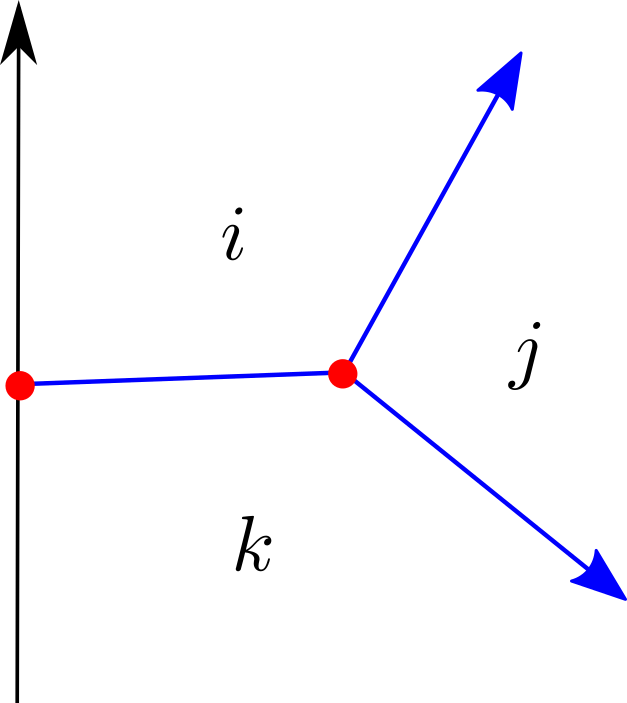
Figure 12: A taut half-plane web which contributes to an off-diagonal element in the differential by inserting the interior amplitude $\beta^{\prime}$ in the bulk vertex.

Suppose the BPS chain complexes on the right configuration are

$$\displaystyle(R^{\prime}_{ij},d^{\prime}_{ij}),(R^{\prime}_{jk},d^{\prime}_{jk}),(R^{\prime}_{ik},d^{\prime}_{ik}).$$ (224)

There are now two half-plane fans of type $ik$, shown in Figure 10 with one and two edges emanating from the boundary vertex respectively. This gives that the morphism spaces are

$$\displaystyle\widehat{R}^{\prime}_{ij} = R^{\prime}_{ij},$$ (225)

$$\widehat{R}^{\prime}_{jk} = R^{\prime}_{jk},$$ (226)

$$\widehat{R}^{\prime}_{ik} = R^{\prime}_{ik}\oplus(R^{\prime}_{ij}\otimes R^{\prime}_{jk}).$$ (227)

Denote the interior amplitude on the right configuration to be

$$\displaystyle\beta^{\prime}_{ijk}\in R^{\prime}_{ij}\otimes R^{\prime}_{jk}\otimes R^{\prime}_{ki}.$$ (228)

Writing an element of $\widehat{R}^{\prime}_{ik}$ as a column vector $\begin{pmatrix}r^{\prime}_{ik}\\ r^{\prime}_{ij}r^{\prime}_{jk}\end{pmatrix}$ the differential on $\widehat{R}^{\prime}_{ik}$ is of the form

$$\displaystyle\widehat{d}^{\prime}_{ik}[\beta^{\prime}] = \begin{pmatrix}d^{\prime}_{ik}&&0\\ M^{\prime}[\beta^{\prime}_{ijk}]&&d^{\prime}_{ijk}\end{pmatrix}$$ (229)

where

$$\displaystyle M^{\prime}[\beta^{\prime}_{ijk}]:R^{\prime}_{ik}\rightarrow R^{\prime}_{ij}\otimes R^{\prime}_{jk}$$ (230)

is a degree $+1$ map defined by Figure 12. Nilpotence of $\widehat{d}^{\prime}_{ik}[\beta^{\prime}]$ holds if

$$\displaystyle d^{\prime}_{ijk}M^{\prime}[\beta^{\prime}_{ijk}]+M^{\prime}[\beta^{\prime}_{ijk}]d^{\prime}_{ik}=0,$$ (231)

therefore we may equivalently view $M^{\prime}[\beta^{\prime}_{ijk}]$ as a chain map

$$\displaystyle M^{\prime}[\beta^{\prime}_{ijk}]:R^{\prime}_{ik}[1]\rightarrow R^{\prime}_{ij}\otimes R^{\prime}_{jk}$$ (232)

and we can rewrite

$$\displaystyle\widehat{R}^{\prime}_{ik}=\text{Cone}\big{(}M^{\prime}[\beta^{\prime}_{ijk}]:R^{\prime}_{ik}[1]\rightarrow R^{\prime}_{ij}\otimes R^{\prime}_{jk}\big{)}.$$ (233)

The only non-trivial multiplication map is

$$\displaystyle i:\widehat{R}^{\prime}_{ij}\otimes\widehat{R}^{\prime}_{jk}\rightarrow\widehat{R}^{\prime}_{ik}$$ (234)

given by inclusion. The $A_{\infty}$ axiom says that $i$ is a chain map with respect to $d^{\prime}_{ijk}$, the product rule differential on $R^{\prime}_{ij}\otimes R^{\prime}_{jk}$ and $\widehat{d}^{\prime}_{ik}[\beta^{\prime}]=d_{M^{\prime}}$ the mapping cone differential on $\widehat{R}^{\prime}_{ik}$.

6.3 Canonical Representatives Satisfy Wall-Crossing Constraint

In this section we show that the canonical representatives (177), (178), (179), (181) satisfy the categorical wall-crossing constraint.

Claim:

Suppose the primed complexes

$$\displaystyle(R^{\prime}_{ij},d^{\prime}_{ij}),(R^{\prime}_{jk},d^{\prime}_{jk}),(R^{\prime}_{ik},d^{\prime}_{ik})$$ (235)

and interior amplitude

$$\displaystyle\beta^{\prime}_{ijk}\in R^{\prime}_{ij}\otimes R^{\prime}_{jk}\otimes R^{\prime}_{kj}$$ (236)

are given as in (177), (178), (179) and (181). Then there is a functor

$$\displaystyle T:\widehat{R}\rightarrow\widehat{R}^{\prime}$$ (237)

which defines a quasi-isomorphism of $A_{\infty}$-categories. We call $T$ the wall-crossing functor.

Proof:

By virtue of the categorical wall-crossing statement, we have the primed morphism spaces

$$\displaystyle\widehat{R}^{\prime}_{ij} = R_{ij},$$ (238)

$$\widehat{R}^{\prime}_{jk} = R_{jk},$$ (239)

$$\widehat{R}^{\prime}_{ik} = R_{ik}\oplus\big{(}R_{ij}\otimes R_{jk}\big{)}[-1]\oplus\big{(}R_{ij}\otimes R_{jk}\big{)}.$$ (240)

The differentials deformed by the interior amplitude component $\beta^{\prime}_{ijk}$ are of the form

$$\displaystyle\widehat{d}^{\prime}_{ik}[\beta^{\prime}] = \widehat{d}_{ik},$$ (241)

$$\widehat{d}^{\prime}_{jk}[\beta^{\prime}] = \widehat{d}_{jk},$$ (242)

$$\widehat{d}^{\prime}_{ik}[\beta^{\prime}] = \begin{pmatrix}d_{ik}&&M[\beta_{ikj}]&&0\\ 0&&d^{[-1]}_{ijk}&&0\\ M^{\prime}_{1}[\beta^{\prime}_{ijk}]&&M^{\prime}_{2}[\beta^{\prime}_{ijk}]&&d_{ijk}\end{pmatrix},$$ (243)

where $M[\beta_{ikj}]$ was defined as before and

$$\displaystyle M^{\prime}_{1}[\beta^{\prime}_{ijk}] : R_{ik}\rightarrow R_{ij}\otimes R_{jk},$$ (244)

$$M^{\prime}_{2}[\beta^{\prime}_{ijk}] : \big{(}R_{ij}\otimes R_{jk}\big{)}[-1]\rightarrow R_{ij}\otimes R_{jk}$$ (245)

are the different components of the maps defined by Figure 12 by inserting $\beta^{\prime}$ in the bulk vertex. The functor $T$ can then be defined as follows. On objects we simply have the identity map. On morphism spaces we define

$$\displaystyle T_{1}:\widehat{R}_{ij}\rightarrow\widehat{R}^{\prime}_{ij},$$ (246)

$$T_{1}:\widehat{R}_{kj}\rightarrow\widehat{R}^{\prime}_{kj}$$ (247)

as identity maps, whereas

$$\displaystyle T_{1}:\widehat{R}_{ik}\rightarrow\widehat{R}^{\prime}_{ik}$$ (248)

is defined as inclusion,

$$\displaystyle T_{1}(r_{ik})=\begin{pmatrix}r_{ik}\\ 0\\ 0\end{pmatrix}$$ (249)

Furthermore

$$\displaystyle T_{2}:\widehat{R}_{ij}\otimes\widehat{R}_{jk}\rightarrow\widehat{R}^{\prime}_{ik}$$ (250)

is again defined to be inclusion, but into the summand with shifted degree,

$$\displaystyle T_{2}(r_{ij}r_{jk})=\begin{pmatrix}0\\ (r_{ij}r_{jk})^{[-1]}\\ 0\end{pmatrix}.$$ (251)

Indeed $(T_{1},T_{2})$ have degrees $(0,-1)$ respectively. The higher maps $T_{n}$ are set to be zero for $n\geq 3$.

First we have to show the axioms of an $A_{\infty}$-morphism are satisfied. Here there are just two axioms to check. At $n=1$ we have to check if $T_{1}$ is a chain map. The only non-trivial check is on the $ik$-component of $T_{1}$ and it follows that we have a chain map from the form of the differential (243). At $n=2$ we must check

$$\displaystyle\begin{split}T_{1}\big{(}m_{2}(r_{ij},r_{jk})\big{)}-m^{\prime}_{2}\big{(}T_{1}(r_{ij}),T_{1}(r_{jk})\big{)}\\ =T_{2}(r_{ij},dr_{jk})\pm T_{2}(dr_{ij},r_{jk})\pm d^{\prime}(T_{2}(r_{ij},r_{jk})).\end{split}$$ (252)

This follows from the following simplification for the expression of $\widehat{d}^{\prime}_{ik}[\beta^{\prime}]$. The explicit form of $\beta^{\prime}$

$$\displaystyle\beta^{\prime}_{ijk}=K^{-1}_{ij}K^{-1}_{jk},$$ (253)

from (181), implies that the off-diagonal maps $M_{1,2}^{\prime}[\beta^{\prime}_{ijk}]$ are

$$\displaystyle M^{\prime}_{1}[\beta_{ijk}^{\prime}] = 0$$ (254)

$$M^{\prime}_{2}[\beta_{ijk}^{\prime}] = \text{id}.$$ (255)

Note that the identity map $M^{\prime}_{2}$ has degree $+1$ due to the degree shift on the domain. Thus we can rewrite the differential as

$$\displaystyle\widehat{d}^{\prime}_{ik}[\beta^{\prime}] = \begin{pmatrix}d_{ik}&&M[\beta_{ikj}]&&0\\ 0&&d^{[-1]}_{ijk}&&0\\ 0&&\text{id}&&d_{ijk}\end{pmatrix}.$$ (256)

Using this expression for $d^{\prime}$ on the right hand side, the axiom easily follows. Thus $T$ defines an $A_{\infty}$-functor.

Finally, we must show that the wall-crossing functor $T$ is a quasi-isomorphism. Again this is non-trivial only on the $ik$-component. The simplification of $\widehat{d}^{\prime}[\beta^{\prime}]$ in fact allows us to relate this to the mapping cylinder construction: similar to (179) one can recognize $\widehat{R}^{\prime}_{ik}$ as the mapping cone of the projection map

$$\displaystyle\pi:R^{\prime}_{ik}[1]=\text{Cone}\big{(}M[\beta_{ikj}]\big{)}[1]\rightarrow R_{ij}\otimes R_{jk}.$$ (257)

In other words we can rewrite

$$\displaystyle\widehat{R}^{\prime}_{ik}=\text{Cyl}\big{(}M[\beta_{ikj}]\big{)}.$$ (258)

Applying the Proposition about mapping cylinders from Appendix A to $f=M[\beta_{ikj}]$ yields that $T$ is a quasi-isomorphism. ∎

Remark

Two $A_{\infty}$-algebras are homotopy equivalent if and only if they are quasi-isomorphic (this is a theorem of Prouté, [Pro]). We can thus say

$$\displaystyle\widehat{R}[X,W]\simeq\widehat{R}^{\prime}[X,W^{\prime}]$$ (259)

where $\simeq$ is meant to be understood as homotopy equivalence.

6.4 Homotopy Equivalence $\implies$ Categorical WCF

Finally we come to the main claim.

Claim

The categorical wall-crossing constraint, namely the homotopy equivalence of $A_{\infty}$-categories

$$\displaystyle\widehat{R}[X,W]\simeq\widehat{R}[X,W^{\prime}]$$ (260)

implies the categorical wall-crossing formula

$$\displaystyle R^{\prime}_{ij} \simeq R_{ij},$$ (261)

$$R^{\prime}_{jk} \simeq R_{jk},$$ (262)

$$R^{\prime}_{ik} \simeq \text{Cone}\big{(}M[\beta_{ikj}]:R_{ij}\otimes R_{jk}\rightarrow R_{ik}\big{)}.$$ (263)

Consider first the $A_{\infty}$ morphism

$$\displaystyle T:\widehat{R}[X,W]\rightarrow\widehat{R}^{\prime}[X,W^{\prime}].$$ (264)

This in particular means that there are chain maps

$$\displaystyle T_{1} : \widehat{R}_{ij}\rightarrow\widehat{R}^{\prime}_{ij},$$ (265)

$$T_{1} : \widehat{R}_{jk}\rightarrow\widehat{R}^{\prime}_{jk},$$ (266)

$$T_{1} : \widehat{R}_{ik}\rightarrow\widehat{R}^{\prime}_{ik}.$$ (267)

We showed in 6.1, 6.2 that the hatted and un-hatted spaces coincide as chain complexes except for $\widehat{R}^{\prime}_{ik}$ which is of the form

$$\displaystyle\widehat{R}^{\prime}_{ik}=\text{Cone}(M^{\prime}[\beta^{\prime}_{ijk}]:R^{\prime}_{ik}[1]\rightarrow R^{\prime}_{ij}\otimes R_{jk}).$$ (268)

Therefore we have chain maps

$$\displaystyle T_{1} : R_{ij}\rightarrow R^{\prime}_{ij},$$ (269)

$$T_{1} : R_{jk}\rightarrow R^{\prime}_{jk},$$ (270)

$$T_{1} : R_{ik}\rightarrow\text{Cone}\big{(}M^{\prime}[\beta^{\prime}_{ikj}]\big{)}.$$ (271)

In addition the $A_{\infty}$-morphism $T$ provides a degree $-1$ map

$$\displaystyle T_{2}:\widehat{R}_{ij}\otimes\widehat{R}_{jk}\rightarrow\widehat{R}^{\prime}_{ik}=\text{Cone}\big{(}M^{\prime}[\beta^{\prime}_{ikj}]\big{)}$$ (272)

such that the second $A_{\infty}$-morphism axiom, (426), which in the present case reads

$$\displaystyle\begin{split}T_{1}\big{(}M[\beta_{ikj}](r_{ij},r_{jk})\big{)}\pm M_{2}^{\prime}\big{(}T_{1}(r_{ij}),T_{1}(r_{jk})\big{)}\\ =\widehat{d}^{\prime}_{ik}[\beta^{\prime}]T_{2}(r_{ij},r_{jk})\pm T_{2}(dr_{ij},r_{jk})\pm T_{2}(r_{ij},dr_{jk}),\end{split}$$ (273)

holds. We showed that $M_{2}^{\prime}$ the bilinear multiplication

$$\displaystyle M_{2}^{\prime}:\widehat{R}^{\prime}_{ij}\otimes\widehat{R}^{\prime}_{jk}\rightarrow\text{Cone}\big{(}M^{\prime}[\beta^{\prime}_{ijk}]\big{)}$$ (274)

is given simply by the inclusion map $i$ in 6.2. We therefore see that the conceptual way to interpret this axiom is that it is saying that the square

$$\displaystyle\begin{CD}R_{ij}\otimes R_{jk}@>{M[\beta_{ikj}]}>{}>R_{ik}\\ @V{T_{1}\otimes T_{1}}V{}V@V{}V{T_{1}}V\\ R^{\prime}_{ij}\otimes R^{\prime}_{jk}@>{i}>{}>\text{Cone}\big{(}M^{\prime}[\beta^{\prime}_{ijk}]\big{)}\end{CD}$$ (275)

commutes up to homotopy

$$\displaystyle i(T_{1}\otimes T_{1})\simeq T_{1}(M[\beta_{ikj}])$$ (277)

with $T_{2}$ providing the chain homotopy. This condition is precisely (152).

Let the morphism in the other direction be

$$\displaystyle S:\widehat{R}^{\prime}[X,W^{\prime}]\rightarrow\widehat{R}[X,W]$$ (278)

which in particular says that we have chain maps

$$\displaystyle S_{1} : R^{\prime}_{ij}\rightarrow R_{ij},$$ (279)

$$S_{1} : R^{\prime}_{jk}\rightarrow R_{jk},$$ (280)

$$S_{1} : \text{Cone}\big{(}M^{\prime}[\beta^{\prime}_{ijk}]\big{)}\rightarrow R_{ik}$$ (281)

that provide homotopy inverses to the $T_{1}$’s. $S$ also provides us with a degree $-1$ map

$$\displaystyle S_{2}:R^{\prime}_{ij}\otimes R^{\prime}_{ik}\rightarrow R_{ik}$$ (282)

that satisfies the second $A_{\infty}$ axiom which in this case says that the the square

$$\displaystyle\begin{CD}R^{\prime}_{ij}\otimes R^{\prime}_{jk}@>{i}>{}>\text{Cone}(M^{\prime}[\beta^{\prime}_{ijk}])\\ @V{S_{1}\otimes S_{1}}V{}V@V{}V{S_{1}}V\\ R_{ij}\otimes R_{jk}@>{}>{M[\beta_{ikj}]}>R_{ik}\end{CD}$$ (283)

commutes up to homotopy, with $S_{2}$ providing the chain homotopy.

$$\displaystyle\begin{CD}R^{\prime}_{ij}\otimes R^{\prime}_{jk}@>{S_{1}\circ i}>{M[\beta]\circ S_{1}\otimes S_{1}}>R_{ik}\end{CD}.$$ (284)

In particular the existence of $(S_{1},T_{1})$ implies that

$$\displaystyle R_{ik} \simeq R^{\prime}_{ik},$$ (285)

$$R_{jk} \simeq R^{\prime}_{jk},$$ (286)

$$R_{ik} \simeq \text{Cone}\big{(}M^{\prime}[\beta^{\prime}_{ijk}]:R^{\prime}_{ik}[1]\rightarrow R^{\prime}_{ij}\otimes R^{\prime}_{jk}\big{)},$$ (287)

which are precisely the homotopy equivalences (149), (150), (151) asserted in the categorical wall-crossing statement. The statement that these are homotopy equivalences follows from the definition of homotopy equivalence of $A_{\infty}$-algebras. Similarly the commutative square above is precisely (153).

Finally we use the Triangularity Lemma from Appendix A.

We found above that

$$\displaystyle R_{ik}\simeq\text{Cone}\big{(}M^{\prime}[\beta^{\prime}_{ijk}]:R^{\prime}_{ik}[1]\rightarrow R^{\prime}_{ij}\otimes R^{\prime}_{jk}\big{)}$$ (288)

so an application of the Triangularity Lemma implies that

$$\displaystyle R^{\prime}_{ik}\simeq\text{Cone}(S_{1}\circ i:R^{\prime}_{ij}\otimes R^{\prime}_{jk}\rightarrow R_{ik}).$$ (289)

Next we recall that the $A_{\infty}$-axiom for $S_{2}$ implies that

$$\displaystyle S_{1}\circ i\simeq M[\beta_{ikj}]\circ(S_{1}\otimes S_{1})$$ (290)

and so their cones are homotopy equivalent. This gives

$$\displaystyle R^{\prime}_{ik}\simeq\text{Cone}\big{(}M[\beta_{ikj}]\circ(S_{1}\otimes S_{1}):R^{\prime}_{ik}\otimes R^{\prime}_{jk}\rightarrow R_{ik}\big{)}.$$ (291)

Finally since

$$\displaystyle S_{1} : R^{\prime}_{ij}\rightarrow R_{ij},$$ (292)

$$S_{1} : R^{\prime}_{jk}\rightarrow R_{jk}$$ (293)

are individually homotopy equivalences, so is

$$\displaystyle S_{1}\otimes S_{1}:R^{\prime}_{ij}\otimes R^{\prime}_{jk}\rightarrow R_{ij}\otimes R_{jk}.$$ (294)

Therefore the latter part has a trivial mapping cone and can be “factored out” to conclude that

$$\displaystyle R^{\prime}_{ik}\simeq\text{Cone}\big{(}M[\beta_{ikj}]:R_{ij}\otimes R_{jk}\rightarrow R_{ik}\big{)},$$ (295)

the result to be shown.

7 The Fermion Degree of a $\zeta$-instanton

Recall that a $\zeta$-instanton with boundary conditions labeled by the triple of solitons

$$\displaystyle\boldsymbol{\phi}=(\phi_{ik},\phi_{kj},\phi_{ji})$$ (296)

that occupy the edges of an $ikj$ wall-crossing triangle contributes to the differential in a categorical wall-crossing process if and only if

$$\displaystyle F(\phi_{ik}\otimes\phi_{kj}\otimes\phi_{ji})=2.$$ (297)

Therefore it is quite important to determine the degree of a given gradient polygon.

By definition the Fermion number is the index of the Dirac operator

$$\displaystyle\mathcal{D}_{\zeta}:\Gamma\big{(}\phi^{*}(TX)\big{)}\rightarrow\Gamma\big{(}\phi^{*}(TX)\big{)}$$ (298)

given by

$$\displaystyle\mathcal{D}_{\zeta}=\begin{pmatrix}\delta^{I}_{J}D_{\bar{s}}^{(1,0)}&&0\\ 0&&\delta^{\bar{I}}_{\bar{J}}D_{s}^{(0,1)}\end{pmatrix}-\begin{pmatrix}0&&\frac{\zeta}{2}g^{I\bar{K}}D_{\bar{K}}\partial_{\bar{J}}\overline{W}\\ \frac{\zeta^{-1}}{2}g^{\bar{I}K}D_{K}\partial_{J}W&&0\end{pmatrix}.$$ (299)

in the background of a $\zeta$-instanton $\phi$ with $\boldsymbol{\phi}$ boundary conditions. Clearly such an index will be difficult to compute if we work directly with $\mathcal{D}$ . However a Maslov index type construction, described in [KKS], gives a more geometric prescription to obtain a well-defined integer $d(\boldsymbol{\phi})$ which is expected to agree with the index of $\mathcal{D}$ up to an overall shift. It would be interesting to prove the equality of $d(\boldsymbol{\phi})$ with the index of $\mathcal{D}$, but this would take us too far afield in the present paper. We proceed assuming the equality holds and use the geometric prescription in what follows. The Maslov index construction also assumes that $X$ is equipped with a nowhere vanishing holomorphic volume form $\Omega$.

Starting from a convex gradient polygon

$$\displaystyle\boldsymbol{\phi}=(\phi_{i_{0}i_{1}},\dots\phi_{i_{n}i_{0}})$$ (300)

the Maslov index prescription gives us $d(\boldsymbol{\phi})\in\mathbb{Z}$ as follows. The main step consists of assigning to the gradient polygon $\boldsymbol{\phi}$ a (homotopy class of a) loop in the Lagrangian Grassmannian of $X$,

$$\displaystyle\text{Lag}(TX)=\{(p,E)|p\in X,\,\,\,E\text{ Lagrangian subspace of }T_{p}X\},$$ (301)

constructed as follows.

First to each soliton $\phi_{ij}$ we associate an open path $\gamma$ in $\text{Lag}(TX)$ simply by taking a point $p$ along the soliton trajectory and assigning to it the Lagrangian subspace

$$\displaystyle T_{p}L_{i}(\zeta_{ij})\subset T_{p}X$$ (302)

as the fiber. Let $\gamma_{k}$ denote the open path assigned to $\phi_{i_{k-1}i_{k}}$ in this way. One notices that the endpoint of $\gamma_{k}$ and the starting point of $\gamma_{k+1}$ have the same base point, the $k$th critical point $i_{k}$, but the Lagrangians fibers differ. The endpoint of $\gamma_{k}$ has fiber

$$\displaystyle\ell_{k}:=T_{i_{k}}L_{i_{k-1}}(\zeta_{i_{k-1}i_{k}})$$ (303)

whereas the starting point of $\gamma_{k+1}$ has the fiber

$$\displaystyle\ell_{k+1}:=T_{i_{k}}L_{i_{k}}(\zeta_{i_{k}i_{k+1}}).$$ (304)

$\ell_{k},\ell_{k+1}$ are Lagrangians living in the same ambient space $T_{i_{k}}X$. Between any two Lagrangian subspaces $L_{1},L_{2}$ in a symplectic vector space $V$, there is a canonical homotopy class of paths $\kappa_{L_{1},L_{2}}$ in $\text{Lag}(V)$ that connects these points, known as the symplectic bridge connecting $L_{1}$ and $L_{2}$. For instance if $\text{dim}(V)=2$, the Lagrangians are specified by points $\theta_{1},\theta_{2}$ in $\mathbb{RP}^{1}\cong S^{1}$ and $\kappa_{\theta_{1},\theta_{2}}$ is the circular arc going in the counter-clockwise direction between these two angles. Therefore there is a well-defined way to connect the open path $\gamma_{k}$ to $\gamma_{k+1}$. Going around the gradient polygon by gluing adjacent open paths via symplectic bridges, one obtains a loop in $\text{Lag}(TX)$.

Next we need to define a winding number of the loop $\gamma$. Let $\bar{\gamma}$ be the loop in $X$ obtained by projecting $\gamma$ to $X$. Thus, if $\bar{\gamma}(t)=p\in X$ then $\gamma(t)\subset T_{p}X$ is a maximal Lagrangian subspace. Let $2n$ denote the rank of $TX$ considered as a real vector bundle over $X$. Then $\gamma(t)$ is a real vector space of dimension $n$. The $n^{\text{th}}$ exterior product of this space is a real line associated to the point $p$. Now, recall that $TX$ can also be considered to be a complex vector bundle of rank $n$. Therefore, the $n^{\text{th}}$ exterior power of $TX$ as a complex vector bundle is a complex line associated to $p$. Indeed, this is the fiber of the canonical bundle at $p$, denoted $\mathcal{K}_{p}$. Note that $\Lambda^{n}\gamma(t)\subset\mathcal{K}_{p}$ is a real line inside a complex line. Finally we use $\Omega$ to trivialize the canonical bundle and therefore get a real line $\ell_{p}\subset\mathbb{C}$. That is, to the loop $\gamma:S^{1}\to{\rm Lag}(TX)$ we associate a loop in $\text{Lag}(\mathbb{C})=\mathbb{RP}^{1}\cong S^{1}$. All-in-all we get a map

$$\displaystyle\psi(\boldsymbol{\phi}):S^{1}\rightarrow\text{Lag}(\mathbb{C})\cong S^{1}.$$ (305)

The integer $d(\boldsymbol{\phi})$ is defined to be the winding number of $\psi(\boldsymbol{\phi})$. The fermion number is then

$$\displaystyle F(\boldsymbol{\phi})=d(\boldsymbol{\phi})+1.$$ (306)

We illustrate the computation of $d(\boldsymbol{\phi})$ in some examples.

7.1 Gradient Polygons in $\mathbb{C}$

Suppose our target space is the complex plane, and say for simplicity that the solitons trace out straight lines so that the gradient polygon $\boldsymbol{\phi}=(\phi_{i_{0}i_{1}},\dots\phi_{i_{n}i_{0}})$ traces out the boundary of an $(n+1)$-gon. This boundary can be clockwise or counter-clockwise oriented and we analyze each case.

For the case of clockwise oriented boundaries, the tangent Lagrangian does not vary along the soliton. The symplectic bridge between $\phi_{i_{k-1}i_{k}}$ and $\phi_{i_{k}i_{k+1}}$ chooses to take the route that takes $\theta_{k}$ radians where $\theta_{k}$ is an internal angle of the polygon. Adding up these angles gives one a total winding number in $S^{1}/\mathbb{Z}_{2}$ of

$$\displaystyle d(\boldsymbol{\phi}) = \frac{\big{(}(n+1)-2\big{)}\pi}{\pi}$$ (307)

$$= n-1$$ (308)

where in the first equality we divide by $\pi$ (not $2\pi$) because of the $\mathbb{Z}_{2}$ quotient. See Figure 13 for the case of $n=2$.

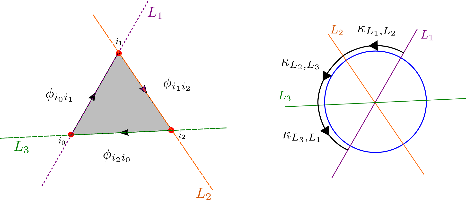
Figure 13: The left shows the gradient polygon $\boldsymbol{\phi}=(\phi_{i_{0}i_{1}},\phi_{i_{1}i_{2}},\phi_{i_{2}i_{0}})$ assumed to trace out straight lines on the complex plane. The dashed lines depict the Lagrangians tangent to these solitons. On the right we show the symplectic bridges $\kappa_{L_{i},L_{i+1}}$ connecting these Lagrangians. The winding number of the total path in $\text{Lag}(\mathbb{C})=S^{1}/\mathbb{Z}_{2}$ is $+1$, therefore $d(\phi)=1$.

For counter-clockwise oriented (convex) polygons , the symplectic bridge chooses to connect adjacent Lagrangians via the route that takes $\pi-\theta_{k}$ radians. This gives one

$$\displaystyle d(\boldsymbol{\phi})=2,$$ (309)

an index independent of $n$.

That clockwise versus counterclockwise give such different answers might be a bit puzzling first, but its origin is clarified if one thinks about the analogous situation in Morse theory. Suppose that $\mathcal{M}(x_{a},x_{b})$ denotes the reduced moduli space of solutions of the gradient flow equation

$$\displaystyle\frac{d\phi^{I}}{dx}=g^{IJ}\frac{\partial h}{\partial\phi^{J}},$$ (310)

between two critical points $x_{a},x_{b}$ of $h$ with Morse indices $\mu_{a},\mu_{b}$ . Then supposing $\mu_{b}>\mu_{a}$ we have

$$\displaystyle\text{dim}\mathcal{M}(x_{a},x_{b})=\mu_{b}-\mu_{a}-1.$$ (311)

On the other hand,

$$\displaystyle\text{dim}\mathcal{M}(x_{b},x_{a})=0.$$ (312)

$\mathcal{M}(x_{b},x_{a})$ is in fact empty, as a consequence of the ascending property of the gradient flow. Thus it should not be very surprising that the moduli space of $\zeta$-instantons is not very well-behaved under orientation reversal of a cyclic fan.

7.2 Paths in $\mathbb{C}^{*}$

Let’s now consider a gradient polygon of solitons in the punctured complex plane $\mathbb{C}^{*}$ so that the total path winds around the origin. We choose the holomorphic volume form that trivializes $T\mathbb{C}^{*}$ to be

$$\displaystyle\Omega=\frac{dX}{X}.$$ (313)

One can show that a loop that winds around the origin, by virtue of this trivialization satisfies

$$\displaystyle d(\boldsymbol{\phi})=0.$$ (314)

This will be useful for the trigonometric Landau-Ginzburg models.

7.3 Fermion Degrees for $\mathbb{Z}_{N}$-symmetric Models

We can use the observations above to determine (integral part of) the fermion degrees of solitons in at least two interesting $\mathbb{Z}_{N}$-symmetric family of models. These are

1. $W=\frac{1}{N+1}\phi^{N+1}-t\phi,$ the deformed $A_{N-1}$ model.

2. $W=\phi+\frac{1}{N-1}\phi^{-(N-1)},$ the $\mathbb{Z}_{N}$ invariant “trigonometric” LG model.

Let’s analyze each one.

7.3.1 Deformed $A_{N-1}$-Model

The model of a single chiral superfield $\phi$ with superpotential

$$\displaystyle W=\frac{1}{N+1}\phi^{N+1}-t\phi$$ (315)

is a well-studied one. The critical points are

$$\displaystyle\phi_{k}=t^{\frac{1}{N}}e^{\frac{2\pi ik}{N}}$$ (316)

for $k=0,1,\dots,N-1$, with critical values

$$\displaystyle W_{k}=-\frac{N}{N+1}t^{\frac{N+1}{N}}e^{\frac{2\pi ik}{N}}.$$ (317)

It is well-known that there is a unique soliton $\phi_{ij}$ interpolating between each pair $(\phi_{i},\phi_{j})$ of distinct critical points. Therefore

$$\displaystyle R_{ij}=\mathbb{Z}\langle\phi_{ij}\rangle.$$ (318)

The degree $F_{ij}$ of $\phi_{ij}$ is of the form

$$\displaystyle F_{ij}=n_{ij}+f_{ij}$$ (319)

where $n_{ij}$ is the integral part and $f_{ij}$ is the fractional part (for which we have a universal formula). It remains to determine $n_{ij}$.

For this we use the constraint coming from the Maslov index: Let $\boldsymbol{\phi}=(\phi_{i_{0}i_{1}},\dots,\phi_{i_{k}i_{0}})$ be a convex gradient polygon. Then

$$\displaystyle n_{i_{0}i_{1}}+n_{i_{1}i_{2}}+\dots+n_{i_{k}i_{0}}=d(\boldsymbol{\phi})+1.$$ (320)

For the present model, we have that

$$\displaystyle(\phi_{i_{0}i_{1}},\phi_{i_{1}i_{2}},\dots\phi_{i_{k}i_{0}})$$ (321)

is a gradient polygon if and only if $i_{0}>i_{1}>i_{2}\dots>i_{n}$ up to cyclic reordering. In the complex plane the gradient polygon traces out a clockwise oriented closed path with $k$-segments, and thus the computation in 7.1 implies

$$\displaystyle d(\phi_{i_{0}i_{1}},\phi_{i_{1}i_{2}},\dots,\phi_{i_{k}i_{0}})=k-2.$$ (322)

We thus get the constraint

$$\displaystyle n_{i_{0}i_{1}}+n_{i_{1}i_{2}}+\dots+n_{i_{k}i_{0}}=k-1,$$ (323)

which is satisfied by a particularly simple solution:

$$\displaystyle n_{ij} = 1\text{ for }i>j,$$ (324)

$$n_{ij} = 0\text{ for }i<j.$$ (325)

By induction on $k$ we see the solution is unique up to shifts

$$\displaystyle n_{ij}\rightarrow n_{ij}+n_{i}-n_{j}.$$ (326)

Therefore we conclude that

$$\displaystyle R_{ij} = \mathbb{Z}[1]\,\text{ for }i>j,$$ (327)

$$R_{ij} = \mathbb{Z}\,\text{ for }i<j.$$ (328)

7.3.2 Trigonometric Models

We can do a similar analysis for the $\mathbb{Z}_{N}$-symmetric trigonometric Landau-Ginzburg models. These have target space $\mathbb{C}^{*}$ and superpotential

$$\displaystyle W=\phi+\frac{1}{N-1}\phi^{-(N-1)}.$$ (329)

The critical points are again located at the roots of unity

$$\displaystyle\phi_{k}=e^{2\pi ik/N}$$ (330)

for $k=0,1,\dots,N-1$ and the critical values are

$$\displaystyle W_{k}=\frac{N}{N-1}e^{\frac{2\pi ik}{N}}.$$ (331)

The soliton spectrum of this model is also known (this model is example $3$ in section $8.1$ of [CV1]): There is a unique soliton between each nearest neighbor pair $(\phi_{i},\phi_{i+1}),(\phi_{i},\phi_{i-1})$ and none between the other pairs. Therefore the only gradient polygon $\boldsymbol{\phi}$ with more than $2$ solitons consists of the full $N$-gon

$$\displaystyle\boldsymbol{\phi}=(\phi_{N-1,N-2},\phi_{N-2,N-3},\dots,\phi_{0,N-1}).$$ (332)

The paths these solitons trace out in $\mathbb{C}^{*}$ consists of round arcs that together wind around the origin once in the clockwise direction. The computation of the Maslov index for paths in $\mathbb{C}^{*}$ allows us to conclude that $d(\boldsymbol{\phi})=0$ and therefore

$$\displaystyle n_{N-1,N-2}+n_{N-2,N-3}+\dots+n_{0,N-1}=1.$$ (333)

We choose the solution

$$\displaystyle n_{i,i-1} = 0,$$ (334)

$$n_{i,i+1} = 1.$$ (335)

Thus the non-zero BPS chain complexes with this solution read

$$\displaystyle R_{i,i+1} = \mathbb{Z}\langle\phi_{i,i+1}\rangle\cong\mathbb{Z},$$ (336)

$$R_{i,i-1} = \mathbb{Z}\langle\phi_{i,i-1}\rangle\cong\mathbb{Z}[1].$$ (337)

8 Examples

Finally let’s illustrate categorical wall-crossing in a few examples.

8.1 Quartic LG Model

Let’s return to the quartic Landau-Ginzburg model that was alluded to in the introduction. The target space is the complex plane $\mathbb{C}$ and the superpotential is

$$\displaystyle W=\frac{1}{4}\phi^{4}-\frac{t_{1}}{2}\phi^{2}-t_{2}\phi.$$ (338)

Consider the point $(t_{1},t_{2})=(0,1)$ where the critical points are

$$\displaystyle\phi_{1}=e^{-\frac{2\pi i}{3}},\,\,\,\,\phi_{2}=1,\,\,\,\,\phi_{3}=e^{\frac{2\pi i}{3}}$$ (339)

with critical values

$$\displaystyle W_{1}=-\frac{3}{4}e^{-\frac{2\pi i}{3}},\,\,\,\,W_{2}=-\frac{3}{4},\,\,\,\,W_{3}=-\frac{3}{4}e^{\frac{2\pi i}{3}}.$$ (340)

The BPS chain complexes consist of

$$\displaystyle R_{12} = \mathbb{Z}\langle\phi_{12}\rangle,$$ (341)

$$R_{13} = \mathbb{Z}\langle\phi_{13}\rangle,$$ (342)

$$R_{23} = \mathbb{Z}\langle\phi_{23}\rangle,$$ (343)

where $\phi_{ij}$ is the unique soliton interpolating between $\phi_{i}$ and $\phi_{j}$. As discussed in 7.3.1, an assignment of degrees consistent with the Maslov index is that all three spaces are concentrated in degree zero.

Now we must count $\zeta$-instantons. Consider the cyclic fan $\{1,3,2\}$ which has degree $+2$. It is argued in papers on domain wall junctions [GT] that there is indeed a solution with no reduced moduli with these trivalent fan boundary conditions. Therefore we have

$$\displaystyle N(\phi_{13},\phi_{32},\phi_{21})=1.$$ (344)

The image swept out by this instanton $\phi(\mathbb{C})$ is depicted in Figure 14.

Figure 14: Image of the $\zeta$-instanton with fan boundary conditions $\{1,3,2\}$ in the $X$-plane. It sweeps out a region bounded by the soliton paths.

Crossing the wall of marginal stability we consider $(t_{1},t_{2})=(1,\epsilon)$ where $\epsilon$ is some small number. Categorical wall-crossing says that the chain complex is

$$\displaystyle R^{\prime}_{13}=\mathbb{Z}\langle(\phi_{12}\phi_{23})^{[-1]}\rangle\oplus\mathbb{Z}\langle\phi_{13}\rangle.$$ (345)

The differential reads

$$\displaystyle d^{\prime}_{13}\big{(}(\phi_{12}\phi_{23})^{[-1]}\big{)} = \phi_{13},$$ (346)

$$d^{\prime}_{13}(\phi_{13}) = 0,$$ (347)

by virtue of the $\zeta$-instanton of Figure 14. Therefore the cohomology is trivial

$$\displaystyle H^{\bullet}(R^{\prime}_{13},d^{\prime}_{13})=0.$$ (348)

Indeed this is the correct BPS Hilbert space on the other side of the wall.

8.2 Trigonometric LG Model

Next we consider the model with target space the complex cylinder $\mathbb{C}^{*}$ with coordinate $\phi$. The family of superpotentials we consider is

$$\displaystyle W=\phi+\lambda\phi^{-1}+\frac{1}{2}\phi^{-2}.$$ (349)

The model at $\lambda=0$ is known in [CV1] as the Bullough-Dodd model and that’s where we begin our analysis. Here we have the critical points

$$\displaystyle\phi_{1}=e^{\frac{2\pi i}{3}},\,\,\,\,\,\phi_{2}=1,\,\,\,\,\,\,\phi_{3}=e^{-\frac{2\pi i}{3}}$$ (350)

with critical values $W_{i}=\frac{3}{2}X_{i}$. As discussed in 7.3.2, there is a single soliton between each pair of vacua and so the BPS chain complexes read

$$\displaystyle R_{12} = \mathbb{Z}\langle\phi_{12}\rangle,$$ (351)

$$R_{23} = \mathbb{Z}\langle\phi_{23}\rangle,$$ (352)

$$R_{13} = \mathbb{Z}\langle\phi_{12}\rangle.$$ (353)

As discussed in 7.2, consistent with the Maslov index is to choose these spaces to be concentrated in degree zero (the vacua have been relabeled compared to that section). Note that there’s a crucial difference with the quartic Landau-Ginzburg model. The vector space associated to the cyclic fan $\{1,2,3\}$ is one-dimensional but now concentrated in degree $+1$. The interior amplitude must therefore be trivial

$$\displaystyle\beta=0.$$ (354)

Therefore, there are no $\zeta$-instantons.

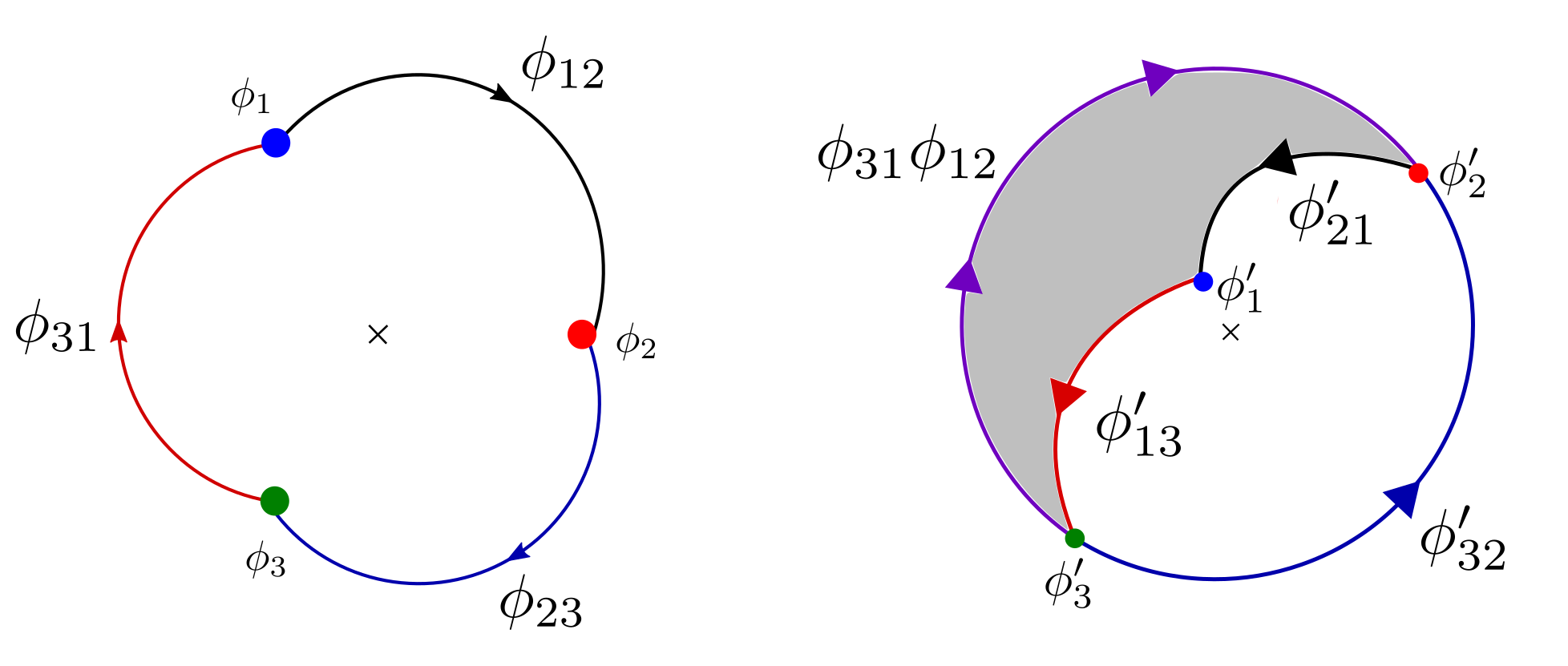
Figure 15: Left: the solitons in the $\lambda=0$ model. There is one between each pair of vacua. On the right we cross the wall of marginal stability and go to $\lambda=2i$. There are now two solitons in the $32$ sector. We also gain a non-trivial $\zeta$-instanton contributing to the interior amplitude.

The absence of $\zeta$-instantons with trivalent boundary conditions may also be geometrically argued as follows. The cyclic fan of solitons sweep out a path that winds around the origin. Were a $\zeta$-instanton to exist, its image would be a region bounded by this path. However, the latter region contains the singular point $\phi=0$, which means that the $\zeta$-instanton blows up at finite $(x,\tau)$.

We now vary $\lambda$ by taking it to be purely imaginary and increasing the magnitude from the $\mathbb{Z}_{3}$ symmetric point $\lambda=0$. The wall of marginal stability is crossed at $\lambda\sim 1.5i$. $W_{1}$ passes through the line between $W_{2}$ and $W_{3}$. Therefore $R_{23}$ jumps. We have

$$\displaystyle R^{\prime}_{23} = (R_{21}\otimes R_{13}\big{)}[-1]\otimes R_{23},$$ (355)

$$= \mathbb{Z}\langle(\phi_{21}\phi_{13})^{[-1]}\rangle\oplus\mathbb{Z}\langle\phi_{23}\rangle,$$ (356)

$$\cong \mathbb{Z}^{2}.$$ (357)

Trivial $\beta$ implies that this is also the cohomology. We see that the $23$ sector has gained a bound state of the $21$ and $13$ sectors.

These two states post wall-crossing have a simple interpretation. When $\lambda$ is large the theory consists of the $\mathbb{CP}^{1}$ mirror along with a vacuum $W_{1}$ running away to infinity. The solitons between $2$ and $3$ are the solitons of this model.

Categorical wall-crossing also predicts the interior amplitude after wall-crossing. Formula (181) says that the interior amplitude should be

$$\displaystyle\beta^{\prime}_{132}=(\phi_{31}\phi_{12})\otimes\phi_{21}\otimes\phi_{13}.$$ (358)

Indeed the geometry of solitons allows the region between the new soliton that appears, $\phi_{31}\phi_{12}$, between $3$ and $2$ and the the old solitons $\phi_{21}$ and $\phi_{13}$ to be filled up by a $\zeta$-instanton. See Figure 15.

8.3 Elliptic LG Model

Let the target space be $T^{2}_{\tau}\backslash\{0\}$ and

$$\displaystyle W=\wp(\phi,\tau).$$ (359)

We study the wall-crossing properties as we vary $\tau$, the complex structure parameter of the torus. The critical points are the familiar half-periods

$$\displaystyle\{\frac{1}{2},\frac{\tau}{2},\frac{1+\tau}{2}\}\text{ mod }\big{(}\mathbb{Z}\oplus\mathbb{Z}\tau\big{)}$$ (360)

with critical values being the elliptic constants

$$\displaystyle\{e_{1}(\tau),e_{2}(\tau),e_{3}(\tau)\}.$$ (361)

It is well-known [CV1, CV2] that this model has precisely two solitons between each pair of critical points, independent of the value of $\tau$. On the other hand, there are still marginal stability walls. For example when $\tau$ is pure imaginary the $e_{i}(\tau)$ are all real and hence co-linear, so the imaginary axis and its $\text{PSL}(2,\mathbb{Z})$-images are marginal stability walls in the upper-half plane. The fact that there are two solitons in any chamber, is explained at the level of BPS indices by the equations

$$\displaystyle 2 = -2+2\cdot 2,\text{ or },$$ (362)

$$-2 = 2-2\cdot 2.$$ (363)

We will now see what happens at the level of chain complexes.

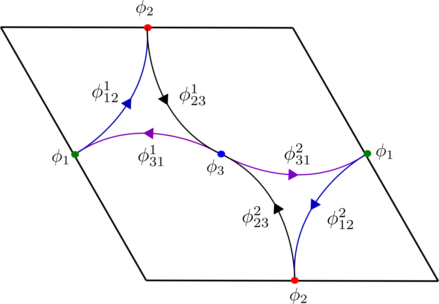
Figure 16: BPS solitons in the $W=\wp(\phi,\tau)$ model with $\tau=e^{\frac{2\pi i}{3}}$. There are two solitons between each pair of vacua, the paths they trace out are depicted.

First work at the $\mathbb{Z}_{3}$ symmetric point $\tau_{0}=e^{\frac{2\pi i}{3}}$. We set

$$\displaystyle\phi_{1}=\frac{\tau_{0}}{2},\,\,\,\,\,\,\,\phi_{2}=\frac{1}{2},\,\,\,\,\,\,\,\phi_{3}=\frac{1+\tau_{0}}{2}.$$ (364)

The homogeneity property of $\wp(\phi,\tau)$ at the $\mathbb{Z}_{3}$ symmetric point implies that the critical values are proportional to the cubic roots of unity

$$\displaystyle W_{1}=W_{0}\,e^{\frac{2\pi i}{3}},\,\,\,\,\,\,\,W_{2}=W_{0},\,\,\,\,\,\,W_{3}=W_{0}\,e^{\frac{-2\pi i}{3}},$$ (365)

where the proportionality constant is, according to [DLMF]:

$$\displaystyle W_{0}=\Bigg{(}\frac{\Gamma^{3}(\frac{1}{3})}{2^{\frac{1}{3}}2\pi}\Bigg{)}^{2}.$$ (366)

The chain complexes are

$$\displaystyle R_{12} = \mathbb{Z}\langle\phi_{12}^{1}\rangle\oplus\mathbb{Z}\langle\phi_{12}^{2}\rangle\cong\mathbb{Z}^{2}[1],$$ (367)

$$R_{13} = \mathbb{Z}\langle\phi_{13}^{1}\rangle\oplus\mathbb{Z}\langle\phi_{13}^{2}\rangle\cong\mathbb{Z}^{2}[1],$$ (368)

$$R_{23} = \mathbb{Z}\langle\phi_{23}^{1}\rangle\oplus\mathbb{Z}\langle\phi_{23}^{2}\rangle\cong\mathbb{Z}^{2}[1].$$ (369)

A computation similar to the deformed $A_{N-1}$-minimal models can be performed to conclude that these chain complexes are all concentrated in degree $+1$ and so all the individual differentials $d_{ij}$ vanish. The trajectories these solitons trace out on $T^{2}_{\tau_{0}}$ are depicted in Figure 16.

The anti-particles are associated to the BPS complexes

$$\displaystyle R_{21} = \mathbb{Z}\langle\phi_{21}^{1}\rangle\oplus\mathbb{Z}\langle\phi_{21}^{2}\rangle\cong\mathbb{Z}^{2},$$ (370)

$$R_{31} = \mathbb{Z}\langle\phi_{31}^{1}\rangle\oplus\mathbb{Z}\langle\phi_{31}^{2}\rangle\cong\mathbb{Z}^{2},$$ (371)

$$R_{32} = \mathbb{Z}\langle\phi_{32}^{1}\rangle\oplus\mathbb{Z}\langle\phi_{32}^{2}\rangle\cong\mathbb{Z}^{2}.$$ (372)

The pairings $K_{12},K_{13},K_{23}$ are diagonal in this basis of solitons.

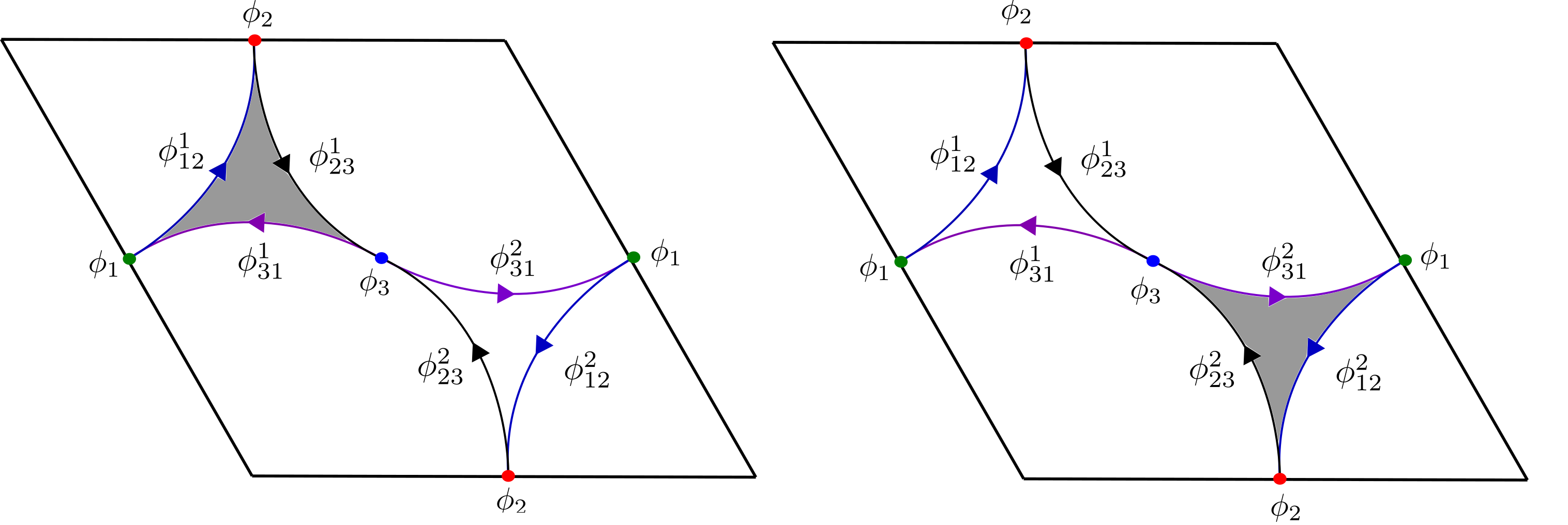
Figure 17: $\zeta$-instantons in the $W=\wp(\phi,\tau)$ model with $\tau=e^{\frac{2\pi i}{3}}$.

Let’s now consider $\zeta$-instantons. The vector space corresponding to the cyclic fan

$$\displaystyle\{1,2,3\},$$ (373)

$R_{12}\otimes R_{23}\otimes R_{31}$ is concentrated in degree $+2$ and so this model allows rigid instantons. There are eight possible gradient polygons $\boldsymbol{\phi}^{a,b,c}=(\phi^{a}_{12},\phi^{b}_{23},\phi^{c}_{31})$ for $a,b,c=1,2$ which could a-priori be occupied. However, the model has additional flavor symmetries whose charges are associated with the winding numbers around the torus . These symmetries reduce the number of possibilities as follows. Denoting $q_{1},q_{2}$ the fugacities for the cycles that (half)-wind around the horizontal and $\tau$-direction respectively, the solitons have the following (exponentiated) winding numbers: States in $R_{12}$ have winding numbers $q_{1}q_{2}$ and $(q_{1}q_{2})^{-1}$, in $R_{23}$ they have $q_{2},q_{2}^{-1}$, and in $R_{13}$ they have $q_{1},q_{1}^{-1}$. On the other hand $\beta$ must have zero winding charge. This cuts down the allowed gradient polygons that can be occupied to

$$\displaystyle\boldsymbol{\phi}^{1} = (\phi_{12}^{1},\phi_{23}^{1},\phi_{31}^{1}),$$ (374)

$$\boldsymbol{\phi}^{2} = (\phi_{12}^{2},\phi_{23}^{2},\phi_{31}^{2}).$$ (375)

The simplest non-trivial guess is to posit that these polygons indeed support $\zeta$-instantons with degeneracies

$$\displaystyle N(\boldsymbol{\phi}^{1}) = 1,$$ (376)

$$N(\boldsymbol{\phi}^{2}) = 1.$$ (377)

Thus we predict the interior amplitude for this model is

$$\displaystyle\beta=\phi^{1}_{12}\otimes\phi^{1}_{23}\otimes\phi^{1}_{31}+\phi^{2}_{12}\otimes\phi^{2}_{23}\otimes\phi^{2}_{31}.$$ (378)

Assuming this is indeed the case, we now evolve from $\tau_{0}=e^{2\pi i/3}$ to, a point of the form $\tau_{1}=ie^{-i\epsilon}$ with $\epsilon>0$. In doing so we must cross the wall at $\text{Re}(\tau)=0$. In such a move, one can check (numerically for instance) that the point $W_{3}$ passes through the line connecting $W_{1}$ and $W_{2}$. Therefore the chain complexes $R_{13},R_{32}$ remain the same as before

$$\displaystyle R^{\prime}_{13} = \mathbb{Z}^{2}[1],$$ (379)

$$R^{\prime}_{32} = \mathbb{Z}^{2},$$ (380)

but $R_{12}$ can jump:

$$\displaystyle R^{\prime}_{12} = \big{(}R_{13}\otimes R_{32}\big{)}[-1]\oplus R_{12}$$ (381)

$$= \big{(}\mathbb{Z}\langle\phi^{1}_{13},\phi^{2}_{13}\rangle\otimes\mathbb{Z}\langle\phi^{1}_{32},\phi^{2}_{32}\rangle\big{)}[-1]\oplus\mathbb{Z}\langle\phi^{1}_{12},\phi^{2}_{12}\rangle.$$ (382)

The first summand is concentrated in degree zero whereas the second factor is in degree one. The $\zeta$-instanton count imply that the differentials act as follows.

$$\displaystyle d^{\prime}_{12}\big{(}(\phi^{1}_{13}\phi^{1}_{32})^{[-1]}\big{)} = \phi^{1}_{12},$$ (383)

$$d^{\prime}_{12}\big{(}(\phi^{1}_{13}\phi^{2}_{32})^{[-1]}\big{)} = 0,$$ (384)

$$d^{\prime}_{12}\big{(}(\phi^{2}_{13}\phi^{1}_{32})^{[-1]}\big{)} = 0,$$ (385)

$$d^{\prime}_{12}\big{(}(\phi^{2}_{13}\phi^{2}_{32})^{[-1]}\big{)} = \phi_{12}^{2}.$$ (386)

Thus the cohomology is

$$\displaystyle H^{\bullet}(R^{\prime}_{12},d^{\prime}_{12})=\mathbb{Z}\langle(\phi^{1}_{13}\phi^{2}_{32})^{[-1]},(\phi^{2}_{13}\phi^{1}_{32})^{[-1]}\rangle,$$ (387)

which is two-dimensional as expected. Categorical wall-crossing has allowed us to see that there has been a non-trivial reorganization of the BPS states in the $12$-sector: in particular their winding numbers jump. This was not visible at the level of ordinary BPS indices.

9 Conclusions and Future Directions

There are various future directions that might be worth pursuing. While staying in the two-dimensional world, it is desirable to categorify more general wall-crossing statements. In particular the presence of twisted masses leads to interesting new phenomena. These new phenomena and how they affect the discussion of categorical wall-crossing will be the subject of a separate paper. Similarly, another interesting direction would be to categorify the beautiful formula of Kontsevich and Soibelman, perhaps by constructing the category of infrared line defects in four-dimensional $\mathcal{N}=2$ theories as a first step.

In a more speculative direction one might wonder about the following. We were studying two-dimensional theories, both in spacetime and from the perspective of the $W$-plane. Edges between vacua in the latter were initially supported by BPS indices, which are integers, and in particular we can use these edges to form a wall-crossing triangle. Categorifying upgraded these integers to chain complexes, but a lesson we learned is that information about these chain complexes by themselves is not sufficient to describe categorical wall-crossing: they must be accompanied by integers associated to the interior of the wall-crossing triangle. In a higher-dimensional generalization of the formalism, let’s say three dimensions, we can imagine having a tetrahedron, whose edges carry categories, faces carry chain complexes and whose interior carries the data of integers. See Figure 18. Wall-crossing would occur when the vertices of the tetrahedron lie on a common plane followed by the apex switching sides as viewed from the base. It would be interesting to spell out the wall-crossing structure of this hierarchy of categories, vector spaces and integers that lie on the various faces of the tetrahedron. Even more compelling would be to find a quantum field theoretic realization of such a higher-dimensional “wall-crossing simplex.”

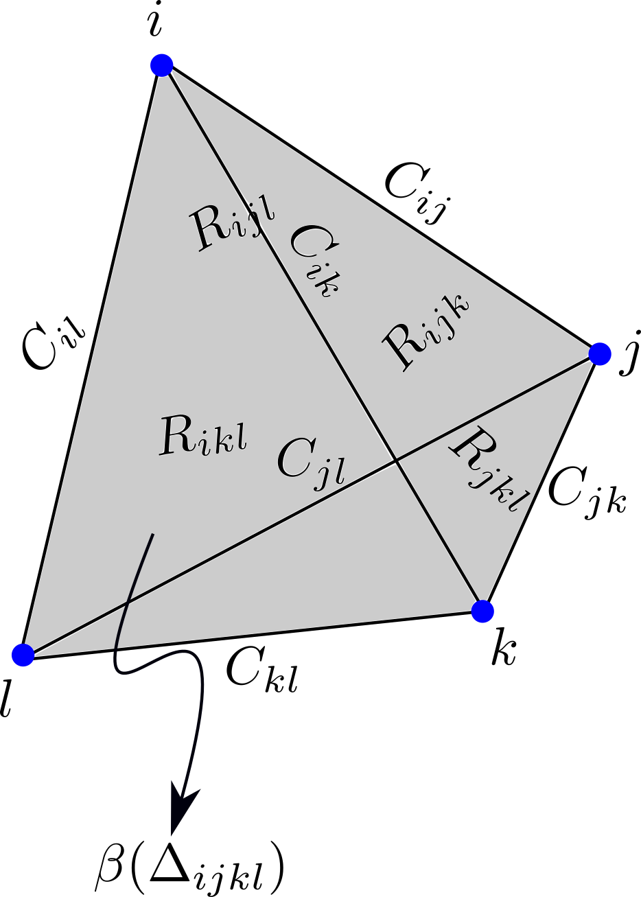
Figure 18: A speculative wall-crossing simplex. $C_{ij}$ etc denote categories associated to edges, $R_{ijk}$ etc denote chain complexes associated to faces and $\beta(\Delta_{ijkl})$ denotes a collection of numbers associated to the interior. Wall-crossing would occur when $i$ passes through the base $jkl$ triangle and moves over to the other side.

In the process of categorifying the simplest wall-crossing formula, we have been lead to an interesting blend of mathematics and physics. The physics of domain wall junctions and their moduli spaces allows one to construct canonical objects in homological algebra: the mapping cone and mapping cylinder. These mathematical objects allow us to compactly express the answer to the question we had initially asked. This is the very essence of physical mathematics.

Appendix A Some Basic Homological Algebra

The categorical wall-crossing formula is most cleanly stated using some standard homological algebra. We summarize the concepts we need below and refer the reader to [Weib] for further details.

Homotopy Equivalence of Complexes

Two complexes $(C,d)$ and $(C^{\prime},d^{\prime})$ are said to be homotopy equivalent if there are chain maps $f:C\rightarrow C^{\prime}$ and $g:C^{\prime}\rightarrow C$ such that

$$\displaystyle gf = 1_{C}+\{d,s\},$$ (388)

$$fg = 1_{C^{\prime}}+\{d^{\prime},s^{\prime}\},$$ (389)

for some degree $-1$ maps $s:C^{\prime}\rightarrow C$ and $s^{\prime}:C\rightarrow C^{\prime}$. $s$ and $s^{\prime}$ are known as chain homotopies.

Mapping Cone Recollection

Given two chain complexes $(A^{\bullet},d_{A})$ and $(B^{\bullet},d_{B})$ along with a chain map

$$\displaystyle f:A^{\bullet}\rightarrow B^{\bullet},$$ (390)

there is a canonical chain complex $\text{Cone}(f)$ defined as follows. The underlying space consists of

$$\displaystyle\text{Cone}(f)=B\oplus A[-1].$$ (391)

Writing an element of $\text{Cone}(f)$ as a column vector

$$\displaystyle\begin{pmatrix}b\\ a^{[-1]}\end{pmatrix},$$ (392)

the differential on $\text{Cone}(f)$ is

$$\displaystyle d[f]=\begin{pmatrix}d_{B}&&f\\ 0&&-d_{A}\end{pmatrix}.$$ (393)

$d[f]$ is nilpotent as a consequence of $f$ being a chain map. The projection map

$$\displaystyle\pi:\text{Cone}(f)\rightarrow A[-1],$$ (394)

and the inclusion map

$$\displaystyle i:B\rightarrow\text{Cone}(f),$$ (395)

are chain maps that fit into the exact sequence

$$\displaystyle\begin{CD}0@>{}>{}>B@>{i}>{}>\text{Cone}(f)@>{\pi}>{}>A[-1]@>{}>{}>0.\end{CD}$$ (396)

Mapping Cylinder Recollection

Suppose we are in the setting of the mapping cone of a morphism $f:A\rightarrow B$, i.e consider $\text{Cone}(f)$. Note that the projection map

$$\displaystyle\pi:\big{(}\text{Cone}(f)\big{)}[1]\rightarrow A$$ (397)

is a chain map. The mapping cylinder of $f$ is then by definition

$$\displaystyle\text{Cyl}(f):=\text{Cone}(\pi).$$ (398)

More explicitly, we can write

$$\displaystyle\text{Cyl}(f)=B\oplus A[-1]\oplus A$$ (399)

The differential on $\text{Cyl}(f)$ reads

$$\displaystyle d=\begin{pmatrix}d_{B}&&f&&0\\ 0&&-d_{A}&&0\\ 0&&\text{id}&&d_{A}\end{pmatrix}.$$ (400)

The following is standard in homological algebra and topology (for instance see Lemma 1.5.6 in Weibel [Weib] ).

Proposition

Suppose $(A,d_{A}),(B,d_{B})$ are chain complexes and $f:A\rightarrow B$ is a chain map. Then $B$ and $\text{Cyl}(f)$ are canonically homotopy equivalent. The map $i:B\rightarrow\text{Cyl}(f)$ is given by inclusion and its homotopy inverse $j:\text{Cyl}(f)\rightarrow B$ is given by

$$\displaystyle j\begin{pmatrix}b\\ a^{[-1]}\\ a^{\prime}\end{pmatrix}=b+f(a^{\prime}).$$ (401)

Remark

The mapping cone and mapping cylinder constructions have their origins in topology. If $f:(X,p_{*})\rightarrow(Y,q_{*})$ is a continuous map of topological spaces we can define topological spaces

$$\displaystyle\text{Cyl}(f) = (X\times I)\cup Y/(x,1)\sim f(x),$$ (402)

$$\text{Cone}(f) = \text{Cyl(f)}/(x,0)\sim p_{*}.$$ (403)

These spaces are related to the previous constructions as follows. If $C_{*}(X),C_{*}(Y)$ denote the singular chain complexes of $X$ and $Y$, then

$$\displaystyle C_{*}(\text{Cyl}(f)) \cong \text{Cyl}\big{(}f_{*}:C_{*}(X)\rightarrow C_{*}(Y)\big{)},$$ (404)

$$C_{*}(\text{Cone}(f)) \cong \text{Cone}\big{(}f_{*}:C_{*}(X)\rightarrow C_{*}(Y)\big{)},$$ (405)

$f_{*}$ being the induced map on complexes.

Triangularity Lemma:

Let $A,B,C$ be chain complexes and $f:A\rightarrow B$ be a chain map. Suppose that

$$\displaystyle\begin{CD}C\simeq\text{Cone}(f:A\rightarrow B)\end{CD}.$$ (406)

Then we can construct chain maps

$$\displaystyle g : B\rightarrow C,$$ (407)

$$h : C[1]\rightarrow A$$ (408)

such that

$$\displaystyle A[-1] \simeq \text{Cone}(g:B\rightarrow C),$$ (409)

$$B \simeq \text{Cone}(h:C[1]\rightarrow A).$$ (410)

The maps $g$ and $h$ can be written down explicitly. We set

$$\displaystyle g=u\circ i$$ (411)

where $u:\text{Cone}(f)\rightarrow C$ is one of the maps provided by homotopy equivalence and $i:B\rightarrow\text{Cone}(f)$ is the inclusion map (also a chain map). Similarly

$$\displaystyle h=\pi\circ v$$ (412)

where $v:C\rightarrow\text{Cone}(f)$ is the homotopy inverse of $u$ and $\pi:\text{Cone}(f)\rightarrow A[-1]$ is the projection map (also a chain map). These maps may be remembered from the commutative diagram

$$\displaystyle\setcounter{MaxMatrixCols}{11}\begin{CD}C\\ @V{v}V{}V\\ 0@>{}>{}>B@>{i}>{}>\text{Cone}(f)@>{\pi}>{}>A[-1]@>{}>{}>0\\ @V{u}V{}V\\ C\end{CD}.$$ (413)

Appendix B $A_{\infty}$ Algebras and Morphisms

This appendix serves as a reminder of some elementary formulas in $A_{\infty}$ theory. We refer the reader to the (unpublished) book of Kontsevich-Soibelman [KoSo4], Keller’s notes [Kel], and appendix A of [GMW] for more details.

$A_{\infty}$-algebra

Given a graded vector space $A$, denote by $T^{\bullet}(A)$ the tensor algebra of $A$, and $T_{+}^{\bullet}(A)$ the positive part of the tensor algebra:

$$\displaystyle T^{\bullet}(A)=\oplus_{n\geq 0}A^{\otimes n},$$ (414)

$$T^{\bullet}_{+}(A)=\oplus_{n\geq 1}A^{\otimes n}.$$ (415)

$A$ is called an $A_{\infty}$-algebra if there is a square-zero, degree one derivation,

$$\displaystyle\delta:T^{\bullet}_{+}(A^{*}[1])\rightarrow T_{+}^{\bullet}(A^{*}[1]).$$ (416)

Extracting Taylor coefficients amounts to a collection maps

$$\displaystyle m_{n}:A^{\otimes n}\rightarrow A$$ (417)

of degree $2-n$ satisfying the $A_{\infty}$-associativity axioms: for each $d\geq 1$ we have

$$\displaystyle\begin{split}\sum_{\begin{subarray}{c}k+l=d+1\\ 1\leq i\leq k\end{subarray}}(-1)^{d_{1}+\dots d_{i-1}-i+1}m_{k}(a_{1},\dots,a_{i-1},m_{l}(a_{i},\dots,a_{i+l-1}),a_{i+l},\dots,a_{d})\\ =0.\end{split}$$ (418)

$a_{i}$ is a homogeneous element and $d_{i}=\text{deg}(a_{i})$.

$A_{\infty}$-morphism

Given two $A_{\infty}$-algebras

$$\displaystyle(A_{1},\{m_{n}\})\text{ and }(A_{2},\{\mu_{n}\})$$ (419)

an $A_{\infty}$-morphism

$$\displaystyle f:A_{1}\rightarrow A_{2}$$ (420)

is an algebra homomorphism (respects tensor algebra structure)

$$\displaystyle f:T^{\bullet}_{+}(A_{2}^{*}[1])\rightarrow T^{\bullet}_{+}(A_{1}^{*}[1])$$ (421)

that is also a chain map: namely $f$ is degree $0$ map satisfying

$$\displaystyle f\delta_{2}=\delta_{1}f.$$ (422)

Again expanding out Taylor coefficients we get a collection of maps

$$\displaystyle f_{n}:(A_{1})^{\otimes n}\rightarrow A_{2}$$ (423)

of degree $1-n$ satisfying the $A_{\infty}$-morphism axioms

$$\displaystyle\begin{split}\sum_{\begin{subarray}{c}k+l=d+1\\ 1\leq i\leq k\end{subarray}}(-1)^{d_{1}+\dots d_{i-1}-i+1}f_{k}(a_{1},\dots,a_{i-1},m_{l}(a_{i},\dots,a_{i+l-1}),a_{i+l},\dots,a_{d})=\\ \sum_{\begin{subarray}{c}n_{1}+\dots+n_{k}=d\\ k\geq 1\end{subarray}}\mu_{k}(f_{n_{1}}(a_{1},\dots,a_{n_{1}}),\dots,f_{n_{k}}(a_{d-n_{k}+1},\dots,a_{d})).\end{split}$$ (424)

The $d=1$ relation is

$$\displaystyle\mu_{1}(f_{1}(a_{1}))=f_{1}(m_{1}(a_{1}))$$ (425)

which simply says that $f_{1}$ is a chain map.

The $d=2$ relation is

$$\displaystyle\begin{split}f_{1}(m_{2}(a_{1},a_{2}))\pm\mu_{2}(f_{1}(a_{1}),f_{1}(a_{2}))=\\ f_{2}(m_{1}(a_{1}),a_{2})\pm f_{2}(a_{1},m_{1}(a_{2}))\pm\mu_{1}(f_{2}(a_{1},a_{2}))\end{split}$$ (426)

where the precise signs can be restored via (424). This says that the diagram

$$\displaystyle\begin{CD}A_{1}^{\otimes 2}@>{f_{1}\otimes f_{1}}>{}>A_{2}^{\otimes 2}\\ @V{m_{2}}V{}V@V{}V{\mu_{2}}V\\ A_{1}@>{}>{f_{1}}>A_{2},\end{CD}$$ (427)

commutes up to homotopy, with $f_{2}$ providing the chain homotopy.

Quasi-isomorphism of $A_{\infty}$-algebras

An $A_{\infty}$-morphism $\{f_{n}\}_{n\geq 1}$ is said to be a quasi-isomorphism if $f_{1}:(A_{1},m_{1})\rightarrow(A_{2},\mu_{1})$ is a quasi-isomorphism of chain complexes.

Homotopy Equivalence of $A_{\infty}$-algebras

Two $A_{\infty}$-morphisms $f,g:A_{1}\rightarrow A_{2}$, between $A_{\infty}$-algebras are said to be homotopic $f\simeq g$, if there is a degree $-1$ map

$$\displaystyle S:T^{\bullet}_{+}(A^{*}_{2}[1])\rightarrow T^{\bullet}_{+}(A^{*}_{1}[1])$$ (428)

such that

$$\displaystyle f-g=S\delta_{2}+\delta_{1}S.$$ (429)

That is $S$ provides a homotopy between the parent maps $f,g$ of the tensor algebra. $A_{1}$ and $A_{2}$ are said to be homotopy equivalent $A_{\infty}$ algebras if there are $A_{\infty}$-morphisms $f:A_{1}\rightarrow A_{2}$ and $g:A_{2}\rightarrow A_{1}$ such that the compositions in either direction are homotopic to the identities on the tensor algebras:

$$\displaystyle g\circ f \simeq 1_{T_{+}A^{*}_{2}},$$ (430)

$$f\circ g \simeq 1_{T_{+}A^{*}_{1}}.$$ (431)

In particular, $(A_{1},m_{1})$ and $(A_{2},\mu_{1})$ are homotopy equivalent chain complexes.

$L_{\infty}$-algebra

A graded vector space $L$ is called an $L_{\infty}$-algebra if there is a derivation differential

$$\delta:S^{\bullet}_{+}(L^{*}[2])\rightarrow S^{\bullet}_{+}(L^{*}[2]).$$

Extracting coefficients gives us that we have a collection of maps

$$\displaystyle\lambda_{n}:L^{\otimes n}\rightarrow L$$ (432)

of degree $3-2n$ which are graded symmetric, and satisfy the $L_{\infty}$-associativity axioms: for each $d\geq 1$ we have

$$\displaystyle\sum_{\begin{subarray}{c}k+l=d+1\\ \sigma\in\text{Sh}_{2}(k-1,l)\end{subarray}}\epsilon(\sigma,\vec{\ell}\,)\lambda_{k}(\lambda_{l}(\ell_{\sigma(1)},\dots,\ell_{\sigma(l)}),\ell_{\sigma(l+1)},\dots,\ell_{\sigma(d)})=0.$$ (433)

In the above $\sigma\in\text{Sh}_{2}(k,l)$ denotes a permutation $\sigma\in S_{k+l}$ such that

$$\displaystyle\sigma(1)<\dots<\sigma(k),\,\,\,\,\sigma(k+1)<\dots<\sigma(k+l).$$ (434)

$L_{\infty}$-morphism

Given

$$\displaystyle(L_{1},\{\lambda_{n}\}),\,\,\,\,\,\,(L_{2},\{\kappa_{n}\})$$ (435)

two $L_{\infty}$-algebras an $L_{\infty}$-morphism $f:L_{1}\rightarrow L_{2}$ is an algebra homomorphism

$$\displaystyle f:S^{\bullet}_{+}(L_{2}^{*}[2])\rightarrow S^{\bullet}_{+}(L_{1}^{*}[2])$$ (436)

that is also a chain map with respect to the $L_{\infty}$-structures. Extracting coefficients we get a collection of maps

$$\displaystyle f_{n}:(L_{1})^{\otimes n}\rightarrow L_{2}$$ (437)

of degree $1-n$ satisfying axioms for an $L_{\infty}$-morphism: for each $d\geq 1$

$$\displaystyle\begin{split}\sum_{\begin{subarray}{c}k+l=d+1\\ \sigma\in\text{Sh}_{2}(k-1,l)\end{subarray}}\epsilon(\sigma,\vec{\ell}\,)f_{k}(\lambda_{l}(\ell_{\sigma(1)},\dots,\ell_{\sigma(l)}),\ell_{\sigma(l+1)},\dots,\ell_{\sigma(d)})=\\ \sum_{\begin{subarray}{c}n_{1}+\dots+n_{k}\\ \sigma\in\text{Sh}_{k}(n_{1},\dots,n_{k})\\ k\geq 1\end{subarray}}\frac{1}{k!}\epsilon^{\prime}(\sigma)\kappa_{n}(f_{n_{1}}(\ell_{\sigma(1)},\dots\ell_{\sigma(n_{1})}),\dots f_{n_{k}}(\ell_{\sigma(d-n_{k}+1)},\dots,\ell_{\sigma(d)})),\end{split}$$ (438)

and $\epsilon(\sigma,\vec{\ell})$ and $\epsilon^{\prime}(\sigma)$ are suitable signs.

Quasi-isomorphism of $L_{\infty}$-algebras

An $L_{\infty}$-morphism $\{f_{n}\}_{n\geq 1}$ from $(L_{1},\{\lambda_{n}\})$ and $(L_{2},\{\kappa_{n}\})$ is said to be a quasi-isomorphism if

$$\displaystyle f_{1}:(L_{1},\lambda_{1})\rightarrow(L_{2},\kappa_{2})$$ (439)

is a quasi-isomorphism of chain complexes.

Maurer-Cartan elements of $L_{\infty}$-algebras

A Maurer-Cartan element $\gamma$ of an $L_{\infty}$ algebra $(L,\{\lambda_{n}\})$ is a degree two element that solves the $L_{\infty}$ Maurer-Cartan equation

$$\displaystyle\sum_{n\geq 1}\frac{1}{n!}\lambda_{n}(\gamma,\dots,\gamma)=0.$$ (440)

An infinitesimal gauge transformation of a Maurer-Cartan element $\gamma$ is written as

$$\displaystyle\delta_{\epsilon}\gamma=\sum_{n\geq 1}\frac{1}{n!}\lambda_{n}(\gamma^{\otimes(n-1)},\epsilon)$$ (441)

where $\epsilon$ is any degree one element of $L$. Indeed one checks that $\gamma+\delta_{\epsilon}\gamma$ solves the Maurer-Cartan equation to first order in $\epsilon$.

Terminology: Algebras vs Categories

In the bulk text of this paper we have often used the terms “algebra” and “category” interchangeably. This is justified because we can go between the two in a precise manner. Following the discussion in chapter 6 of [KoSo4], given a linear category with a finite object set $S$, we can define a unital algebra to be

$$\displaystyle A=\oplus_{r,s\in S}\text{Hom}(r,s),$$ (442)

with the unit being the direct sum of identity compositions and multiplications given by compositions of morphisms. Conversely, if a unital algebra $A$ is equipped with commuting idempotents $\{\Pi_{i}\}_{i\in I}$ such that $1_{A}=\oplus_{i}\Pi_{i}$, then we can construct a category $\mathcal{C}$ by setting the object set to be $I$ and letting

$$\displaystyle\text{Hom}(i,j)=\Pi_{i}A\,\Pi_{j}.$$ (443)

Appendix C $N_{ij}\in\{0,1\}$ for $W\in\mathbb{C}[X]$

We give a proof of the assertion that a Landau-Ginzburg model with target $\mathbb{C}$ and $W(X)$ a Morse polynomial has at most a single soliton between any pair of critical points. For this we consider the relative homology group

$$\displaystyle V=H_{1}(\mathbb{C},\text{Re}(\zeta^{-1}W)\rightarrow\infty;\mathbb{Z})$$ (444)

where $\zeta$ is a phase not equal to any of the critical phases. $V$ is easily constructed. Supposing that the degree of $W$ is $n$, we divide the complex plane $\mathbb{C}$ into $2n$ wedges of equal angle $\frac{2\pi}{n}$ and shade alternating regions $R_{1},\dots,R_{n}$. A basis for $V$ is provided by cycles $\gamma_{a,a+1}$ that connect $R_{a}$ and $R_{a+1}$ for $a=1,\dots,n-1$. On the other hand, Picard-Lefschetz theory says that the homology class of the Lefschetz thimbles $L_{i}(\zeta)$ for $i=1,\dots,n-1$ critical points of $W$ must also form a $\mathbb{Z}$-module basis for $V$. In particular this implies that if $L_{i}(\zeta)$ connects $R_{a},R_{b}$ and $L_{j}(\zeta)$ connects $R_{c},R_{d}$ then $\{a,b\}\neq\{c,d\}$ since otherwise they will be multiples of each other by $\pm 1$ in homology, and thus linearly dependent elements of $V$. Considering a point $p$ on the $\zeta$-ray emanating from $W_{i}$ far out enough, $W^{-1}(p)\cap L_{i}(\zeta)$ is a pair of points lying in distinct regions $R_{a},R_{b}$ which are connected by $L_{i}$. Therefore $|L_{i}(\zeta_{ji}e^{-i\epsilon})\cap L_{j}(\zeta_{ji}e^{i\epsilon})|$ is at most one, concluding the proof.

References

- [ADJM] E. Andriyash, F. Denef, D. L. Jafferis and G. W. Moore, “Wall-crossing from supersymmetric galaxies,” JHEP 01, 115 (2012) doi:10.1007/JHEP01(2012)115 [arXiv:1008.0030 [hep-th]].
- [Aur] D. Auroux, “A beginner’s introduction to Fukaya categories,” [arXiv:1301.7056 [math.SG]].
- [BC] R. Bergamin and S. Cecotti, “FQHE and geometry,” JHEP 12, 172 (2019) doi:10.1007/JHEP12(2019)172 [arXiv:1910.05022 [hep-th]].
- [CGGLPFZ] A. Carey, F. Gesztesy, H. Grosse, G. Levitina, D. Potapov, F. Sukochev, D. Zanin, “Trace Formulas for a Class of non-Fredholm Operators: A Review,” Reviews in Mathematical Physics 28, No. 10 (2016) 1630002 [arXiv:1610.04954 [math.AP]].
- [CHT] S. M. Carroll, S. Hellerman and M. Trodden, “Domain wall junctions are 1/4 - BPS states,” Phys. Rev. D 61, 065001 (2000) doi:10.1103/PhysRevD.61.065001 [arXiv:hep-th/9905217 [hep-th]].
- [Cec] S. Cecotti, “Trieste Lectures on Wall–Crossing Invariants,” https://people.sissa.it/~cecotti/ictptext.pdf
- [CFIV] S. Cecotti, P. Fendley, K. A. Intriligator and C. Vafa, “A New supersymmetric index,” Nucl. Phys. B 386, 405-452 (1992) doi:10.1016/0550-3213(92)90572-S [arXiv:hep-th/9204102 [hep-th]].
- [CV1] S. Cecotti and C. Vafa, “On classification of N=2 supersymmetric theories,” Commun. Math. Phys. 158, 569-644 (1993) doi:10.1007/BF02096804 [arXiv:hep-th/9211097 [hep-th]].
- [CV2] S. Cecotti and C. Vafa, “Ising model and N=2 supersymmetric theories,” Commun. Math. Phys. 157, 139-178 (1993) doi:10.1007/BF02098023 [arXiv:hep-th/9209085 [hep-th]].
- [DM] F. Denef and G. W. Moore, “Split states, entropy enigmas, holes and halos,” JHEP 11, 129 (2011) doi:10.1007/JHEP11(2011)129 [arXiv:hep-th/0702146 [hep-th]].
- [DLMF] “Digital Library of Mathematical Functions,” https://dlmf.nist.gov/23.5
- [Dor] N. Dorey, “The BPS spectra of two-dimensional supersymmetric gauge theories with twisted mass terms,” JHEP 11, 005 (1998) doi:10.1088/1126-6708/1998/11/005 [arXiv:hep-th/9806056 [hep-th]].
- [GMN1] D. Gaiotto, G. W. Moore and A. Neitzke, “Four-dimensional wall-crossing via three-dimensional field theory,” Commun. Math. Phys. 299, 163-224 (2010) doi:10.1007/s00220-010-1071-2 [arXiv:0807.4723 [hep-th]].
- [GMN2] D. Gaiotto, G. W. Moore and A. Neitzke, “Framed BPS States,” Adv. Theor. Math. Phys. 17, no.2, 241-397 (2013) doi:10.4310/ATMP.2013.v17.n2.a1 [arXiv:1006.0146 [hep-th]].
- [GMN3] D. Gaiotto, G. W. Moore and A. Neitzke, “Wall-Crossing in Coupled 2d-4d Systems,” JHEP 12, 082 (2012) doi:10.1007/JHEP12(2012)082 [arXiv:1103.2598 [hep-th]].
- [GMW] D. Gaiotto, G. W. Moore and E. Witten, “Algebra of the Infrared: String Field Theoretic Structures in Massive Field Theory In Two Dimensions,” [arXiv:1506.04087 [hep-th]].
- [GMWSh] D. Gaiotto, G. W. Moore and E. Witten, “An Introduction To The Web-Based Formalism,” [arXiv:1506.04086 [hep-th]].
- [GT] G. W. Gibbons and P. K. Townsend, “A Bogomolny equation for intersecting domain walls,” Phys. Rev. Lett. 83, 1727-1730 (1999) doi:10.1103/PhysRevLett.83.1727 [arXiv:hep-th/9905196 [hep-th]].
- [HIV] K. Hori, A. Iqbal and C. Vafa, “D-branes and mirror symmetry,” [arXiv:hep-th/0005247 [hep-th]].
- [MS1] K. Hori, S. Katz, A. Klemm, R. Pandharipande, R. Thomas, C. Vafa, R. Vakil and E. Zaslow, “Mirror symmetry.”
- [INOS] K. Ito, M. Naganuma, H. Oda and N. Sakai, “An Exact solution of BPS junctions and its properties,” Nucl. Phys. B Proc. Suppl. 101, 304-313 (2001) doi:10.1016/S0920-5632(01)01515-8 [arXiv:hep-th/0012182 [hep-th]]
- [KS] H. Kajiura and J. Stasheff, “Homotopy algebras inspired by classical open-closed string field theory,” Commun. Math. Phys. 263, 553-581 (2006) doi:10.1007/s00220-006-1539-2 [arXiv:math/0410291 [math.QA]].
- [KKS] M. Kapranov, M. Kontsevich and Y. Soibelman, “Algebra of the infrared and secondary polytopes,” Adv. Math. 300, 616-671 (2016) doi:10.1016/j.aim.2016.03.028 [arXiv:1408.2673 [math.SG]].
- [Kel] B. Keller, “Introduction to A-infinity algebras and modules,” [arXiv:math/9910179 [math.RA]].
- [KoSo1] M. Kontsevich and Y. Soibelman, “Stability structures, motivic Donaldson-Thomas invariants and cluster transformations,” [arXiv:0811.2435 [math.AG]].
- [KoSo2] M. Kontsevich and Y. Soibelman, “Motivic Donaldson-Thomas invariants: Summary of results,” [arXiv:0910.4315 [math.AG]].
- [KoSo3] M. Kontsevich and Y. Soibelman, “Lectures on motivic Donaldson-Thomas invariants and wall-crossing formulas.”
- [KoSo4] M. Kontsevich and Y. Soibelman, “Deformation Theory. I.”
- [LY] K. M. Lee and P. Yi, “Dyons in N=4 supersymmetric theories and three pronged strings,” Phys. Rev. D 58, 066005 (1998) doi:10.1103/PhysRevD.58.066005 [arXiv:hep-th/9804174 [hep-th]].
- [M1] G. Moore, “2010 PiTP Lectures,” http://www.physics.rutgers.edu/~gmoore/PiTP-LectureNotes.pdf, https://video.ias.edu/pitp-2010
- [M2] G. Moore, “Framed BPS States In Four And Two Dimensions,” http://www.physics.rutgers.edu/~gmoore/StringMath2016L.pdf, http://www.physics.rutgers.edu/~gmoore/StringMath2016-Aspen.pdf, http://www.physics.rutgers.edu/~gmoore/Hamburg2019-Short.pdf.
- [N] A. Neitzke, “PCMI Lectures on BPS States and Spectral Networks.”
- [Pio] B. Pioline, “Four ways across the wall,” J. Phys. Conf. Ser. 346, 012017 (2012) doi:10.1088/1742-6596/346/1/012017 [arXiv:1103.0261 [hep-th]].
- [Pro] A. Prouté, “Algèbres différentielles fortement homotopiquement associatives”, Thèse d’Etat, Université Paris VII, 1984.
- [Seib] N. Seiberg, “The Power of holomorphy: Exact results in 4-D SUSY field theories,” [arXiv:hep-th/9408013 [hep-th]].
- [SW] N. Seiberg and E. Witten, “Electric - magnetic duality, monopole condensation, and confinement in N=2 supersymmetric Yang-Mills theory,” Nucl. Phys. B 426, 19-52 (1994) doi:10.1016/0550-3213(94)90124-4 [arXiv:hep-th/9407087 [hep-th]].
- [Seid] P. Seidel “Fukaya categories and Picard-Lefschetz theory,” Zurich Lectures in Advanced Mathematics. European Mathematical Society (EMS), Zürich
- [Weib] C. Weibel, “An Introduction to Homological Algebra,” Cambridge Studies in Advanced Mathematics.
- [Wit1] E. Witten, “Dynamical Breaking of Supersymmetry,” Nucl. Phys. B 188, 513 (1981) doi:10.1016/0550-3213(81)90006-7
- [Wit2] E. Witten, “Supersymmetry and Morse theory,” J. Diff. Geom. 17, no.4, 661-692 (1982)