Using graph theory to compute Laplace operators arising in a model for blood flow in capillary networks

Abstract

Maintaining cerebral blood flow is critical for adequate neuronal function. Previous computational models of brain capillary networks have predicted that heterogeneous cerebral capillary flow patterns result in lower brain tissue partial oxygen pressures. It has been suggested that this may lead to number of diseases such as Alzheimer’s disease, acute ischemic stroke, traumatic brain injury and ischemic heart disease. We have previously developed a computational model that was used to describe in detail the effect of flow heterogeneities on tissue oxygen levels. The main result in that paper was that, for a general class of capillary networks, perturbations of segment diameters or conductances always lead to decreased oxygen levels. This result was varified using both numerical simulations and mathematical analysis. However, the analysis depended on a novel conjecture concerning the Laplace operator of functions related to the segment flow rates and how they depend on the conductances. The goal of this paper is to give a mathematically rigorous proof of the conjecture for a general class of networks. The proof depends on determining the number of trees and forests in certain graphs arising from the capillary network.

1 Introduction

Maintaining cerebral blood flow is critical for adequate neuronal function [3, 4]. Previous computational models of brain capillary networks have predicted that heterogeneous cerebral capillary flow patterns result in lower brain tissue partial oxygen pressures [5]. It has been suggested that this may lead to number of diseases such as Alzheimer’s disease, acute ischemic stroke, traumatic brain injury and ischemic heart disease [6, 7].

In [9], we developed a computational model that was used to describe in detail the effect of flow heterogeneities on tissue oxygen levels. The primary question addressed in [9] was: How do the oxygen levels depend on changes in network parameters such as segment diameters and conductances? In particular, if we randomly perturb a given choice of parameters, will the oxygen levels, on average, increase or decrease? The main result in [9] was that, for a general class of capillary networks, perturbations of segment diameters or conductances always lead to decreased oxygen levels.

This result was varified using both numerical simulations and mathematical analysis. However, the analysis depended on a novel conjecture concerning the Laplace operator of functions related to the segment flow rates and how they depend on the conductances. The goal of this paper is to give a mathematically rigorous proof of the conjecture for a class of networks.

An outline of the paper is the following. In the next section, we state our conjecture, as well as the main results. In Section 3, we present the model for capillary blool flow developed in [9] and discuss how results presented in this paper are related to those given in [9]. The results depend on computing the Laplace operator of certain functions, which depend on the flow rates. In Section 4, we compute explicit formulas for these Laplacians. In Section 5, we describe numerical simulations, which demonstrate that the conjecture holds for a general class of capillary networks. Finally, in Section 6, we rigorously prove that the conjecture holds for a specific class of networks. The proof depends on determining the number of trees and forests in certain graphs arising from the capillary network.

2 Statement of main results

Blood flow in brain capillary networks is often modeled using an undirected, weighted graph. Suppose that this graph has K nodes, which we denote as simply 1, 2, …, K. Each node has degree greater than one, except for nodes corresponding to where blood either enters or leaves the network. These nodes have degree one.

To each edge $e_{ij}$, connecting nodes $i$ and $j$, we assign a conductance, $\alpha_{ij}$. Moreover, to each node $i$, there corresponds a blood pressure, $P_{i}$. We assume that the blood pressures at the incoming and outgoing nodes are given. Then the remaining blood pressures are determined by assuming conservation of blood flow at each node. That is, the blood flow rate along some edge $e_{ij}$ is given by

$$Q_{ij} = \alpha_{ij}(P_{i}-P_{j}).$$ (1)

We assume that for each node $i$, the sum of all the blood flow rates along edges from node $i$ is zero. This leads to a linear algebra problem (which is described in detail later) for the remaining blood pressures.

For each edge $e_{ij}$, let $\Gamma_{ij}=1/Q_{ij}$. Note that each $\Gamma_{ij}$ is a function of all the conductances $\alpha_{rs}$. Let $\Delta$ be the Laplace operator. That is,

$$\Delta\Gamma_{ij} = \sum_{r,s}\frac{\partial^{2}\Gamma_{ij}}{\partial\alpha_{rs}^{2}}.$$

Our conjecture is then

Main Result: Let $e_{ij}$ be any edge with $P_{i}-P_{j}>0$. Then $\Delta\Gamma_{ij}$, evaluated when all the conductances are equal, is positive.

This result is varified for a general class of networks using numerical simulations and for a specific class of networks using rigorous mathematical analysis.

3 Motivation of the Main Result

Here we briefly describe the model for capillary blool flow developed in [9] and discuss how results presented in this paper are related to those given in [9].

We begin with a graph as described above, except we now assume that there is just one incoming node, at $N_{in}$. We assign a conductance $\alpha_{ij}$ to each edge $e_{ij}$ and blood pressures to the incoming and outgoing nodes. We then compute blood pressures, $P_{i}$, at all of the nodes and flow rates, $Q_{ij}$, along each of the edges, as described above.

To each node, $i$, there also corresponds an oxygen partial pressure, $\Omega_{i}$. These are determined as follows. We assume that $\Omega_{Nin}$ is given at the incoming node. Suppose that $e_{ij}$ is some edge with $P_{i}>P_{j}$ so that $Q_{ij}>0$. We parameterize this edge by the distance, $x$, from node $i$ and assume that along this edge, $\Omega_{ij}(x)$ decays according to an equation of the form

$$\frac{d\Omega_{ij}}{dx} = -\frac{\rho}{Q_{ij}}\,F(\Omega_{ij})$$ (2)

with $\Omega_{ij}(0)=\Omega_{i}$. Here $\rho$ is a fixed parameter and $F$ is simply assumed to be a positive, smooth function. We need some rule to determine how $\Omega_{j}$ is computed at each node, $j$. If there is just one node $i$ with $Q_{ij}>0$, then $\Omega_{j}=\Omega_{ij}(l_{ij})$ where $l_{ij}$ is the length of edge $e_{ij}$. If there are two nodes $i$ and $k$ so that $Q_{ij}>0~{}{\rm and}~{}Q_{kj}>0$, then $\Omega_{j}\,=\,C_{1}\,\Omega_{ij}(l_{ij})+C_{2}\,\Omega_{kj}(l_{kj})$ for some positive constants $C_{1}~{}{\rm and}~{}C_{2}$.

In [9], we show that random perturbations of conductances lead, on average, to a decrease in oxygen levels. More precisely, suppose that the conductances along the edge $e_{ij}$ are given by $\alpha_{ij}^{0}$. For $\epsilon>0$, we say that $\{\alpha_{ij}\}$ is an $\epsilon$-perturbation of $\{\alpha_{ij}^{0}\}$ if $|\alpha_{ij}-\alpha_{ij}^{0}|<\epsilon$ for each edge. We assume that $0<\epsilon<{\rm min}\{\alpha_{ij}^{0}\}$. For a given set of conducctances, $\{\alpha_{ij}\}$, we can compute the oxygen partial pressure $\Omega_{i}$ at each of the nodes. Let $\Omega_{i\epsilon}$ equal to the average oxygen partial pressure at node $i$ taken over all $\epsilon$-perturbations of $\{\alpha_{ij}^{0}\}$.

The main result in [9] is that if the $\{\alpha_{ij}^{0}\}$ are all some fixed constant and the parameter $\rho$, which appears in (2), is sufficiently small, then $\Omega_{i\epsilon}<\Omega_{i0}$ at each node $i$.

This result was demonstrated by noting that the oxygen levels $\Omega_{i}$ are all functions of the conductances $\alpha_{rs}$. We showed numerically in [9] that for a general class of networks, $\Delta\,\Omega_{i}\,<\,0$ at each node. Here, $\Delta$ is the Laplace operater with respect to the conductance variables. It then follows from the so-called Maximum Principle for the Laplace operator that each $\Omega_{i}$ is greater than the average value of the oxygen levels over all perturbations of the conductances of a fixed size; that is, $\Omega_{i\epsilon}<\Omega_{i0}$ at each node $i$.

A key step in the analysis of this result was to consider $\Gamma_{ij}\,=\,1/Q_{ij}$, as defined above. In [9], we proved the following

Proposition: If $\Delta\,\Gamma_{ij}\,>\,0$ for each edge $e_{ij}$ with $P_{i}\,-\,P_{j}\,>\,0$ and $\rho$ is sufficiently small, then $\Delta\Omega_{i}\,<\,0$ for each node.

Hence, the Main Result of this paper plays a central role in analyzing the model presented in [9].

4 Computation of $\Delta\Gamma_{ij}$

Here we assume that there is just one incoming node and one outgoing node; these are $N_{in}=K~{}{\rm and}~{}N_{out}=K-1$, respectively. It is straightforward to extend the formulas which follow if there are multiple incoming or outgoing nodes.

Let $\cal{A}$ be the $(K-2)\times(K-2)$ matrix defined by

$${\cal A}_{ij}=\left\{\begin{array}[]{cl}-\alpha_{ij}&{\rm if}~{}~{}i\neq j\\ \sum_{k=1}^{K}\alpha_{ik}&{\rm if}~{}~{}i=j.\end{array}\right.$$

Here, $\alpha_{ij}=0$ if there is no edge connecting nodes $i~{}{\rm and}~{}j$. Let $I_{in}~{}{\rm and}~{}I_{out}$ be the nodes that share edges with the incoming and outgoing nodes, respectively, $P_{in}~{}{\rm and}~{}P_{out}$ be the blood pressures at the incoming and outgoing nodes and $\cal{B}$ be the $(K-2)\times 1$ column matrix

$${\cal B}_{i,1}=\left\{\begin{array}[]{cl}\alpha_{lin,N-1}~{}P_{in}&{\rm if}~{}~{}i=I_{in}\\ \alpha_{lout,N}~{}~{}P_{out}&{\rm if}~{}~{}i=I_{out}\\ 0&{\rm otherwise.}\end{array}\right.$$

Then the blood pressures ${\cal P}\,=\,(P_{1},P_{2},...,P_{K-2})$ satisfy ${\cal A}\,{\cal P}\,=\,{\cal B}.$

We solve for the $P_{i}$ using Cramer’s rule. For each $i$, with $1\leq i\leq K-2$, let ${\cal D}^{i}$ be the matrix in which the $i^{\rm th}$ column of $\cal A$ is replaced with $\cal B$, $\delta={\rm det}~{}\cal A$ and $\delta_{i}={\rm det}~{}{\cal D}^{i}$. Then $P_{i}~{}=~{}\delta_{i}/\delta.$

Note that $\delta$ and each $\delta_{i}$ are linear functions of the conductances, $\alpha_{rs}$. Hence, for each conductance $\alpha_{rs}$, we can write

$$\delta = \alpha_{rs}A^{1}_{rs}+A^{0}_{rs}~{}~{}~{}{\rm and}~{}~{}~{}\delta_{i}~{}=~{}\alpha_{rs}D^{i1}_{rs}+D^{i0}_{rs}$$

where $A^{1}_{rs},\,A^{0}_{rs},\,D^{i1}_{rs}~{}{\rm and}~{}D^{i0}_{rs}$ do not depend on $\alpha_{rs}$. It follows that if $1\leq i,j\leq K-2$, then for each $\alpha_{rs}$,

$$\Gamma_{ij} = \frac{1}{Q_{ij}}~{}=~{}\frac{1}{\alpha_{ij}(P_{i}-P_{j})}$$

$$= \frac{1}{\alpha_{ij}}\left(\frac{\alpha_{rs}A^{1}_{rs}+A^{0}_{rs}}{\alpha_{rs}(D^{i1}_{rs}-D^{j1}_{rs})+(D^{i0}_{rs}-D^{j0}_{rs})}\right).$$

If $\alpha_{ij}\neq\alpha_{rs}$, then

$$\frac{\partial^{2}\,\Gamma_{ij}}{\partial\,\alpha^{2}_{rs}} = -2(D^{i1}_{rs}-D^{j1}_{rs})\left(\frac{A^{1}_{rs}~{}(D^{i0}_{rs}-D^{j0}_{rs})-A^{0}_{rs}~{}(D^{i1}_{rs}-D^{j1}_{rs})}{\alpha_{ij}(\delta_{i}-\delta_{j})^{3}}\right).$$ (3)

If $\alpha_{ij}=\alpha_{rs}$, then $D_{rs}^{j1}=D_{rs}^{j1}$ and

$$\frac{\partial^{2}\,\Gamma_{ij}}{\partial\,\alpha^{2}_{rs}} = \frac{2A^{0}_{rs}}{\alpha_{rs}^{3}(\delta_{i}-\delta_{j})}.$$ (4)

Now suppose that $i=K-1~{}{\rm and}~{}j=I_{in}$. Then $P_{i}=P_{in}$. If $\alpha_{ij}\neq\alpha_{rs}$, then

$$\frac{\partial^{2}\,\Gamma_{ij}}{\partial\,\alpha^{2}_{rs}} = -2(P_{in}A^{1}_{rs}-D^{j1}_{rs})\left(\frac{A^{1}_{rs}~{}(P_{in}A^{0}_{rs}-D^{j0}_{rs})-A^{0}_{rs}~{}(P_{in}A^{1}_{rs}-D^{j1}_{rs})}{\alpha_{ij}~{}(P_{in}\delta-\delta_{j})^{3}}\right).$$

If $\alpha_{ij}=\alpha_{rs}$, then $P_{in}A^{1}_{rs}=D^{j1}_{rs}$ and

$$\frac{\partial^{2}\Gamma_{ij}}{\partial\alpha^{2}_{rs}} = \frac{2A^{0}_{rs}}{\alpha_{rs}^{3}(P_{in}\delta-\delta_{j})}.$$ (6)

Finally, suppose that $i=I_{out}~{}{\rm and}~{}j=K$. Then $P_{j}=P_{out}$. If $\alpha_{ij}\neq\alpha_{rs}$, then

$$\frac{\partial^{2}\,\Gamma_{ij}}{\partial\,\alpha^{2}_{rs}} = -2(D^{i1}_{rs}-P_{out}A^{1}_{rs})\left(\frac{A^{1}_{rs}~{}(D^{i0}_{rs}-P_{out}A^{0}_{rs})-A^{0}_{rs}~{}(D^{i1}_{rs}-P_{out}A^{1}_{rs})}{\alpha_{ij}~{}(\delta_{i}-P_{out}\delta)^{3}}\right)$$

If $\alpha_{ij}=\alpha_{rs}$, then $P_{out}A^{1}_{rs}=D^{j1}_{rs}$ and

$$\frac{\partial^{2}\Gamma_{ij}}{\partial\alpha^{2}_{rs}} = \frac{2A^{0}_{rs}}{\alpha_{rs}^{3}(\delta_{i}-P_{out}\delta)}.$$ (8)

5 Voronoi Networks

We numerically computed $\Delta\Gamma_{ij}$ for a class of networks, as shown in Figure 1A. This graph corresponds to a Voronoi diagram with 4 $\times$ 4 cells. To generate a Voronoi diagram with M $\times$ N cells, we choose random points

$$(x_{j},y_{k})\in\{(x,y):j-1<x<j,~{}k-1<y<k\}$$

where $1\leq j\leq M$ and $1\leq k\leq N$. These points are then used to generate a Voronoi diagram within Matlab. We next remove those edges that intersect the region outside the rectangle $\{(x,y):0<x<M,~{}0<y<N\}$. Finally, we add incoming and outgoing nodes and edges as follows. Suppose that the nodes of the diagram constructed so far are at $\{(x_{i},y_{k})\}$. Choose nodes $min~{}{\rm and}~{}max$ so that the remaining nodes satisfy $y_{min}<y_{k}<y_{max}$. The incoming edge then connects the point $(x_{max},N+1)$ with the node at $(x_{max},y_{max})$. The outgoing edge connects the point $(x_{min},0)$ with the node at $(x_{min},y_{min}).$

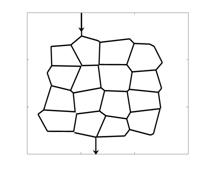
Figure 1: Voronoi network

For each $M~{}{\rm and}~{}N$ with $1\leq M,\,N\leq 5$, we computed $\Delta\Gamma_{ij}$ for each edge in 1000 randomly chosen Voronoi networks of size $M\times N$. In every case, $\Delta\Gamma_{ij}>0$.

6 Grid Networks

We now consider the graph shown in Figure 2B, which we denote as ${\cal G}_{N}$. We will rigoursly prove that the Main Result is valid for all $N\geq 0$.

6.1 Trees and Forests

We assume, without loss of generality, $P_{in}=1~{}{\rm and}~{}P_{out}=0$. If, in addition, each conductance $\alpha_{ij}=1$, then we can rewrite (3) as

$$\frac{\partial^{2}\,\Gamma_{ij}}{\partial\,\alpha^{2}_{rs}} = 2\left(1-\frac{D^{i0}_{rs}-D^{j0}_{rs}}{\delta_{i}-\delta_{j}}\right)\left(\frac{\delta}{\delta_{i}-\delta_{j}}\right)\left(\frac{A^{0}_{rs}}{\delta}-\frac{D^{i0}_{rs}-D^{j0}_{rs}}{\delta_{i}-\delta_{j}}\right).$$ (9)

One can interpret each term in (9) as the number of trees and forests of some graph [1]. If $\gamma~{}{\rm and}~{}\beta$ are any distinct edges, let

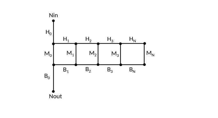
Figure 2: The network ${\cal G}_{N}$

• ${\cal T}_{N}~{}=$ the number of trees of ${\cal G}_{N}$.

• $\sigma_{N}~{}=$ the number of 2-forests of ${\cal G}_{N}$ so that $N_{in}~{}{\rm and}~{}N_{out}$ are in different trees.

• $\sigma_{N}(\gamma)~{}=$ the number of 2-forests of ${\cal G_{N}}\backslash\gamma$ so that $N_{in}~{}{\rm and}~{}N_{out}$ are in different trees.

• ${\cal P}_{N}(\beta)~{}=$ the number of trees in ${\cal G}_{N}$ so that the unique path from $N_{in}$ to $N_{out}$ passes through $\beta$.

• ${\cal P}_{N}(\gamma,\beta)~{}=$ the number trees in ${\cal G}_{N}\backslash\gamma$ so that the unique path from $N_{in}$ to $N_{out}$ passes through $\beta$.

If $\gamma\neq\beta$ correspond to the edges $e_{rs}~{}{\rm and}~{}e_{ij}$, respectively, then for each $N$,

$$\delta = \sigma_{N},~{}~{}~{}~{}~{}~{}~{}~{}A^{0}_{rs}\,=\,\sigma_{N}(\gamma),$$

$$\delta_{i}-\delta_{j} = {\cal P}_{N}(\beta),~{}~{}~{}D^{i0}_{rs}-D^{j0}_{rs}\,=\,{\cal P}_{N}(\gamma,\beta).$$

Hence, we can rewrite (9) as

$$\frac{\partial^{2}\,\Gamma_{\beta}}{\partial\,\gamma^{2}} = 2\left(1-\frac{{\cal P}_{N}(\gamma,\beta)}{{\cal P}_{N}(\beta)}\right)\left(\frac{\sigma_{N}}{{\cal P}_{N}(\beta)}\right)\left(\frac{\sigma_{N}(\gamma)}{\sigma_{N}}-\frac{{\cal P}_{N}(\gamma,\beta)}{{\cal P}_{N}(\beta)}\right).$$ (10)

In a similar manner, we can rewrite (4) and (4) as (10). If $\gamma=\beta$, then we can rewrite (4), (6) and (8) as

$$\frac{\partial^{2}\,\Gamma_{\beta}}{\partial\,\gamma^{2}} = 2\,\frac{\sigma_{N}(\beta)}{{\cal P}_{N}(\beta)}.$$ (11)

6.2 Formulas

The following formulas are derived in Section 7. These results are illustrated in Figure 3.

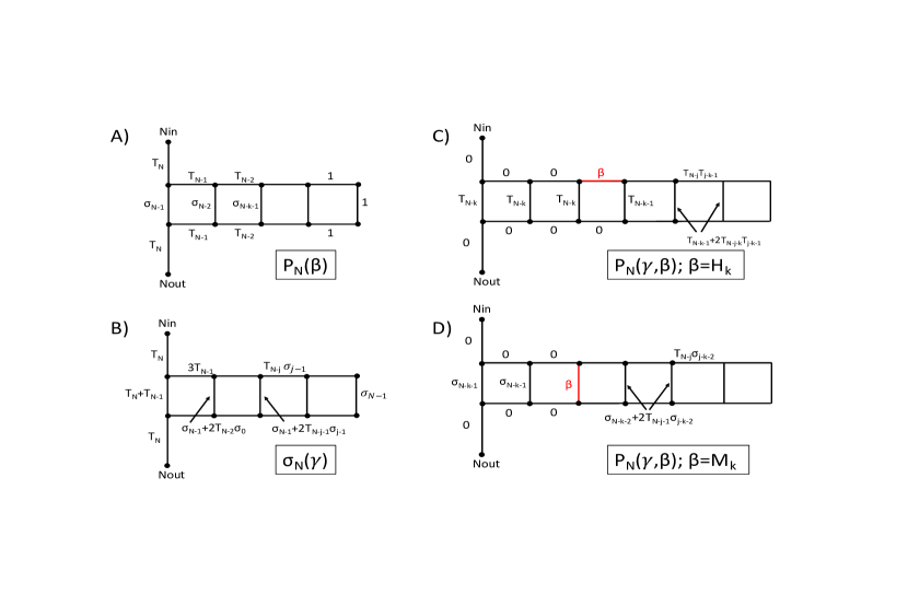
Figure 3: A) ${\cal P}_{N}(\beta)$. B) $\sigma_{N}(\gamma)$. C) ${\cal P}_{N}(\gamma,\beta);~{}\beta=H_{K}$. D) ${\cal P}_{N}(\gamma,\beta);~{}\beta=M_{K}$.

(F1)   $T_{N+1}=4\,T_{N}-T_{N-1};~{}~{}~{}~{}T_{0}=1,~{}T_{1}=4.$

(F2)   $\sigma_{N+1}=4\,\sigma_{N}-\sigma_{N-1};~{}~{}~{}~{}\sigma_{0}=3,~{}\sigma_{1}=11.$

(F3)

$${\cal P}_{N}(\beta)= T_{N-k} {\rm if}~{}\beta=H_{k}~{}{\rm or}~{}B_{k}$$

$$\sigma_{N-k-1} {\rm if}~{}\beta=M_{k}.$$

(F4)

$$\sigma_{N}(\gamma)= T_{N-j}\,\sigma_{j-1} {\rm if}~{}\gamma=H_{j}~{}{\rm or}~{}B_{j}$$

$$\sigma_{N-1}+2T_{N-j-1}\sigma_{j-1} {\rm if}~{}\gamma=M_{j}.$$

(F5)   If $\beta=H_{k}$ or $B_{k}$ and $\gamma=M_{j}$, then

$${\cal P}_{N}(\gamma,\beta)= T_{N-k} {\rm if}~{}0\leq j\leq k-1$$

$$T_{N-k-1} {\rm if}~{}j=k$$

$$T_{N-k-1}+2\,T_{N-j-k}\,T_{j-k-1} {\rm if}~{}k<j\leq N.$$

(F6)   If $\beta=H_{k}$ or $B_{k}$ and $\gamma=H_{j}$ or $B_{j}$, then

$${\cal P}_{N}(\gamma,\beta)= 0 {\rm if}~{}0\leq j\leq k$$

$$T_{N-j}\,T_{j-k-1} {\rm if}~{}k+1\leq j\leq N.$$

(F7)   If $\beta=M_{k}$ and $\gamma=M_{j}$, then

$${\cal P}_{N}(\gamma,\beta)= \sigma_{N-k-1} {\rm if}~{}0\leq j\leq k$$

$$\sigma_{N-k-2}+2T_{N-j-1}\sigma_{j-k-2} {\rm if}~{}k+1\leq j\leq N.$$

(F8)   If $\beta=M_{k}$ and $\gamma=H_{j}$ or $B_{j}$, then

$${\cal P}_{N}(\gamma,\beta)= 0 {\rm if}~{}0\leq j\leq k$$

$$T_{N-j}\,\sigma_{j-k-2} {\rm if}~{}k+1\leq j\leq N.$$

6.3 Some useful identities

The following identities will be used throughout the analysis:

A1)   $T_{N+1}=T_{N}+\sigma_{N}$.

A2)   $\lim_{N\rightarrow\infty}\frac{T_{N}}{T_{N+1}}~{}=~{}\lim_{N\rightarrow\infty}\frac{\sigma_{N}}{\sigma_{N+1}}~{}=~{}x_{*}\equiv 2-\sqrt{3}.$

A3)   $\frac{T_{N}}{T_{N+1}}\,<\,x_{*}\,<\,\frac{\sigma_{N}}{\sigma_{N+1}}\,<\,3/11$. Moreover, $\frac{T_{N}}{T_{N+1}}~{}{\rm and}~{}\frac{\sigma_{N}}{\sigma_{N+1}}$ are increasing and decreasing functions of $N$, respectively.,

A4)   $\lim_{N\rightarrow\infty}\frac{T_{N}}{\sigma_{N}}~{}=~{}\frac{x_{*}}{1-x_{*}}$.

A5)   If $0\leq k<j\leq N$, then $\frac{T_{j-k-1}}{T_{N-k}}~{}<~{}\frac{\sigma_{j-1}}{\sigma_{N}}.$

A6)   $\sigma_{k}\,x_{*}^{k}\,>\,2.5$ for all $k\geq 0$.

A7)   ${\cal P}(\gamma,\beta)\,\leq\,{\cal P}(\beta)$ for every pair of edges $\beta~{}{\rm and}~{}\gamma$.

The proof of A1) is by induction. It is true when $N=0$ since $T_{0}=1,\,T_{1}=4~{}{\rm and}~{}\sigma_{0}=3$. Suppose that 1 is true up to some $N$. Then using (F1) and (F2),

$$T_{N+1} = T_{N}+\sigma_{N}~{}\Rightarrow~{}4T_{N+1}=4T_{N}+4\sigma_{N}$$

$$\Rightarrow T_{N+2}+T_{N}=T_{N+1}+T_{N-1}+\sigma_{N+1}+\sigma_{N_{1}}$$

$$\Rightarrow T_{N+2}=T_{N+1}+\sigma_{N+1.}$$

To prove A2), let $x_{N}=\frac{T_{N}}{T_{N+1}}$ or $\frac{\sigma_{N}}{\sigma_{N+1}}$. Then (F1) implies that $x_{N+1}=1/(4-x_{N})$. As $N\rightarrow\infty$, $x_{N}$ approaches the stable fixed point of this map. This fixed point satisfies $x_{*}^{2}-4x_{*}+1=0$. That is, $x_{*}=2-\sqrt{3}$.

To prove A3), let $x_{N}=\frac{T_{N}}{T_{N+1}}$. Then $x_{0}=1/4<x_{*}$. Moreover, if $x_{N}<x_{*}$, then

$$x_{N+1}~{}=~{}4-\frac{1}{x_{N}}\,>\,x_{N}$$

and

$$x_{N+1}~{}=~{}4-\frac{1}{x_{N}}\,<\,4-\frac{1}{x_{*}}\,=\,x_{*}$$

A similar argument hold for $\frac{\sigma_{N}}{\sigma_{N+1}}$. Moreover, $\frac{\sigma_{N}}{\sigma_{N+1}}\,<\,\frac{\sigma_{0}}{\sigma_{1}}=3/11$.

To prove A4), note that

$$\frac{T_{N}}{\sigma_{N}}~{}=~{}\frac{T_{N}}{T_{N+1}-T_{N}}~{}=~{}\frac{T_{N}/T_{N+1}}{1-T_{N}/T_{N+1}}~{}\rightarrow\frac{x_{*}}{1-x_{*}}$$

as $N\rightarrow\infty$.

A5) follows from A3) because

$$\frac{T_{j-k-1}}{T_{N-k}} = \frac{T_{j-k-1}}{T_{j-k}}\frac{T_{j-k}}{T_{j-k+1}}\dots\frac{T_{N-k-1}}{T_{N-k}}$$

$$< \frac{T_{j-1}}{T_{j}}\frac{T_{j}}{T_{j+1}}\dots\frac{T_{N-1}}{T_{N}}~{}~{}~{}<~{}~{}\frac{\sigma_{j-1}}{\sigma_{j}}\frac{\sigma_{j}}{\sigma_{j+1}}\dots\frac{\sigma_{N-1}}{\sigma_{N}}$$

$$= \frac{\sigma_{j-1}}{\sigma_{N}}$$

To prove A6), let $B_{k}=\sigma_{k}\,x_{*}^{k}$. Then

$$B_{k+1} = \sigma_{k+1}\,x_{*}^{k+1}~{}=~{}4\,\sigma_{k}\,{}_{*}^{k+1}\,-\,\sigma_{k-1}\,x_{*}^{k+1}$$

$$= 4\,x_{*}\,B_{k}\,-\,x_{*}^{2}\,B_{k-1}$$

$$= 4\,x_{*}\,(B_{k}\,-\,B_{k-1})\,+\,B_{k-1}.$$

Since $x_{*}^{2}-4x_{*}-1=0$. Hence,

$$\frac{B_{k+1}\,-\,B_{k-1}}{B_{k}\,-\,B_{k-1}} = 4x_{*}$$

and, therefore,

$$\frac{B_{k+1}\,-\,B_{k}}{B_{k}-B_{k-1}} = 4x_{*}\,-\,1~{}=~{}x_{*}^{2}.$$

Hence, for all $k\geq 0$.

$$B_{k+1} = B_{k}\,+\,x_{*}^{2}\,(B_{k}\,-\,B_{k-1}).$$

Since $B_{0}=3~{}{\rm and}~{}B_{1}=11x_{*}<B_{0}$, it follows that

$$B_{k} = B_{1}\,+\,(B_{1}\,-\,B_{0})\,\sum_{i=1}^{2(k-1)}x_{*}^{2i}$$

$$> B_{1}\,+\,(B_{1}\,-\,B_{0})\,\sum_{i=1}^{\infty}x_{*}^{2i}$$

$$= B_{1}\,+\,(B_{1}\,-\,B_{0})\left(\frac{x_{*}^{2}}{1-x_{*}^{2}}\right)$$

$$\approx 2.9434~{}>~{}2.5.$$

Finally, A7) is true because every tree in ${\cal G}\backslash\gamma$ such that the unique path from $N_{in}$ to $N_{out}$ passes through $\beta$ is also a tree in ${\cal G}$ with the same property.

6.4 Derivatives

We now use (10) and (11) to compute second derivatives. There are many cases to consider.

1. $\beta=H_{k}$ or $B_{k}$ and $\gamma=H_{j},~{}0\leq j<k$. Then

   $${\cal P}_{N}(\beta)=T_{N-k},~{}~{}~{}\sigma_{N}(\gamma)=T_{N-j}\,\sigma_{j-1},~{}~{}~{}{\cal P}(\gamma,\beta)=0.$$

   Hence,

   $$\frac{\partial^{2}\,\Gamma_{\beta}}{\partial\,\gamma^{2}} = 2\,\frac{T_{N-j}~{}\sigma_{j-1}}{T_{N-k}}~{}>~{}0.$$

2. $\beta=H_{k}$ or $B_{k}$ and $\gamma=H_{j},~{}k<j\leq N$. Then

   $${\cal P}_{N}(\beta)=T_{N-k},~{}~{}~{}\sigma_{N}(\gamma)=T_{N-j}\,\sigma_{j-1},~{}~{}~{}{\cal P}_{N}(\gamma,\beta)=T_{N-j}\,T_{j-k-1}.$$

   Hence, using the Identities A5 and A7,

   $$\frac{\partial^{2}\,\Gamma_{\beta}}{\partial\,\gamma^{2}} = 2\left(1-\frac{{\cal P}_{N}(\gamma,\beta)}{{\cal P}_{N}(\beta)}\right)\,\left(\frac{\sigma_{N}\,T_{N-j}}{T_{N-k}}\right)\left(\frac{\sigma_{j-1}}{\sigma_{N}}-\frac{T_{j-k-1}}{T_{N-k}}\right).$$

   $$> 0.$$

3. $\beta=H_{k}$ or $B_{k}$ and $\gamma=M_{j},~{}0\leq j\leq k-1$. Then ${\cal P}_{N}(\beta)\,=\,{\cal P}_{N}(\gamma,\beta)=T_{N-k}$. Hence,

   $$\frac{\partial^{2}\,\Gamma_{\beta}}{\partial\,\gamma^{2}} = 0$$

4. $\beta=H_{k}$ or $B_{k}$ and $\gamma=M_{j},~{}k+1\leq j\leq N$. Then

   $${\cal P}_{N}(\beta)=T_{N-k},~{}~{}~{}{\cal P}(\gamma,\beta)=T_{N-k-1}+2\,T_{N-j-k}\,T_{j-k-1},~{}~{}~{}\sigma_{N}(\gamma)=\sigma_{N-1}+2\,T_{N-j-1}\sigma_{j-1}.$$

   Hence, using Identites A5 and A7,

   $$\frac{\partial^{2}\,\Gamma_{\beta}}{\partial\,\gamma^{2}} = \Lambda_{1}\,\Lambda_{2}$$

   where

   $$\Lambda_{1} = 2\,\left(\frac{\sigma_{N}}{T_{N-k}}\right)\,\left(1-\frac{{\cal P}_{N}(\gamma,\beta)}{{\cal P}_{N}(\beta)}\right)~{}>~{}0$$

   and

   $$\Lambda_{2} = \frac{\sigma_{N-1}+2\,T_{N-j-1}\sigma_{j-1}}{\sigma_{N}}\,-\,\frac{T_{N-k-1}+2\,T_{N-j-k}\,T_{j-k-1}}{T_{N-k}}$$

   $$= \left(\frac{\sigma_{N-1}}{\sigma_{N}}-\frac{T_{N-k-1}}{T_{N-k}}\right)\,+\,2\,T_{N-j-1}\,\left(\frac{\sigma_{j-1}}{\sigma_{N}}-\frac{T_{j-k-1}}{T_{N-k}}\right)$$

   $$> 0.$$

5. $\beta=M_{k}$ and $\gamma=H_{j}$ or $B_{j},0\leq j\leq k$. Then

   $${\cal P}_{N}(\beta)=\sigma_{N-k-1},~{}~{}~{}{\cal P}_{N}(\gamma,\beta)=0,~{}~{}~{}\sigma_{N}(\gamma)=T_{N-j}\,\sigma_{j-1}.$$

   Hence,

   $$\frac{\partial^{2}\,\Gamma_{\beta}}{\partial\,\gamma^{2}} = 2\,\frac{T_{N-j}\,\sigma_{j-1}}{\sigma_{N-k-1}}.$$

   Note that $T_{N-j}\,\sigma_{j-1}$ is a decreasing function of $j$. This is because, from Identity A3,

   $$\frac{\sigma_{j-1}}{\sigma_{j}}~{}>~{}x_{*}~{}>~{}\frac{T_{N-j-1}}{T_{N-j}}.$$

   Hence,

   $$\frac{\partial^{2}\,\Gamma_{\beta}}{\partial\,\gamma^{2}} > 2\,\frac{T_{N-k}\,\sigma_{k-1}}{\sigma_{N-k-1}}.$$

6. $\beta=M_{k}$ and $\gamma=H_{j}$ or $B_{j},~{}k<j\leq N$. Then

   $${\cal P}_{N}(\beta)=\sigma_{N-k-1}~{}~{}~{}{\cal P}_{N}(\gamma,\beta)=T_{N-j}\,\sigma_{j-k-2},~{}~{}~{}\sigma_{N}(\gamma)=T_{N-j}\,\sigma_{j-1}.$$

   Hence,

   $$\frac{\partial^{2}\,\Gamma_{\beta}}{\partial\,\gamma^{2}} = 2\,\Lambda_{1}\,\Lambda_{2}\,\Lambda_{3}\,\Lambda_{4}$$

   where

   $$\Lambda_{1} = 1-\frac{{\cal P}_{N}(\gamma,\beta)}{{\cal P}_{N}(\beta)};~{}~{}~{}~{}~{}\Lambda_{2}=\frac{T_{N-j}\,\sigma_{j-1}}{\sigma_{N-k-1}};$$

   $$\Lambda_{3} = \frac{\sigma_{N}}{\sigma_{N-k-1}};~{}~{}~{}~{}~{}~{}~{}~{}~{}~{}~{}~{}\Lambda_{4}=\frac{\sigma_{N-k-1}}{\sigma_{N}}-\frac{\sigma_{j-k-2}}{\sigma_{j-1}}.$$

   From Identity A7 , $0<\Lambda_{1}<1$. It was shown earlier that $T_{N-j}\,\sigma_{j-1}$ is a decreasing function of $j$. Since $j>k$,

   $$0~{}<~{}\Lambda_{2}~{}<~{}\frac{T_{N-k}\,\sigma_{k-1}}{\sigma_{N-k-1}}.$$

   Using Identity A3,

   $$\Lambda_{3} < \frac{\sigma_{N}}{\sigma_{N-1}}\,\frac{\sigma_{N-1}}{\sigma_{N-2}}\dots\frac{\sigma_{N-k-2}}{\sigma_{N-k-1}}$$

   $$< x_{*}^{-(k+1)}.$$

   Now consider $\Lambda_{4}$. Let

   $$A_{j}~{}=~{}\frac{\sigma_{j-k-1}}{\sigma_{j}}.$$

   Then

   $$A_{j+1} = \frac{\sigma_{j-k}}{\sigma_{j+1}}~{}=~{}\frac{4\,\sigma_{j-k-1}-\sigma_{j-k-2}}{4\,\sigma_{j}-\sigma_{j-1}}$$

   $$= \frac{A_{j}-x_{j}\,A_{j-1}}{1-x_{j}}$$

   $$= A_{j}+\lambda_{j}\,(A_{j}-A_{j-1})$$

   where

   $$x_{j} = \frac{\sigma_{j-1}}{4\,\sigma_{j}}~{}~{}~{}{\rm and}~{}~{}~{}\lambda_{j}\,=\,\frac{x_{j}}{1-x_{j}}\,=\,\frac{\sigma_{j-1}}{\sigma_{j+1}}.$$

   Let   $\epsilon=A_{k+1}\,-\,A_{k}.$ Then, for $n\geq 1$,

   $$A_{k+n} = A_{k+1}\,+\,\epsilon\,\sum_{i=1}^{n-1}\prod_{y=1}^{i}\lambda_{k+y}.$$

   Hence,

   $$A_{N}\,-\,A_{j-1} = \epsilon\,\left(1+\sum_{i=1}^{N-j-1}\prod_{y=1}^{i}\lambda_{j+y}\right)\prod_{y=k+1}^{j-1}\lambda_{y}.$$

   From Identity A3, $\lambda_{j}<y_{*}^{2}$ where $y_{*}=3/11$. Moreover,

   $$\epsilon = \ A_{k+1}\,-\,A_{k}~{}=~{}\frac{3}{\sigma_{k+1}}-\frac{1}{\sigma_{k}}$$

   $$= \frac{3\sigma_{k}-\sigma_{k+1}}{\sigma_{k}\,\sigma_{k+1}}~{}=~{}\frac{\sigma_{k-1}-\sigma_{k}}{\sigma_{k}\,\sigma_{k+1}}~{}<~{}0.$$

   This implies that  $\frac{\partial^{2}\,\Gamma_{\beta}}{\partial\,\gamma^{2}}\,<\,0$   and ,   $|\epsilon|\,<\,\frac{1}{\sigma_{k+1}}.$   It follows that

   $$|\Lambda_{4}| = |A_{N}-A_{j-1}|~{}<~{}|\epsilon|\,y_{*}^{2\,(j-k+1)}\,\sum_{i=0}^{\infty}y_{*}^{2i}$$ (12)

   $$< \frac{y_{*}^{2\,(j-k-1)}}{\sigma_{k+1}\,(1-y_{*}^{2})}.$$

   We have therefore shown that

   $$\left|\frac{\partial^{2}\,\Gamma_{\beta}}{\partial\,\gamma^{2}}\right| < 2\,\left(\frac{T_{N-k}\,\sigma_{k-1}}{\sigma_{N-k-1}}\right)\left(\frac{1}{x_{*}^{k+1}\,\sigma_{k+1}}\right)\left(\frac{y_{*}^{2\,(j-k-1)}}{1-y_{*}^{2}}\right)$$

   $$< .8\,\left(\frac{T_{N-k}\,\sigma_{k-1}}{\sigma_{N-k-1}}\right)\left(\frac{y_{*}^{2\,(j-k-1)}}{1-y_{*}^{2}}\right).$$

   Here we used Identity A6.

7. $\beta=M_{k}$ and $\gamma=M_{j},~{}0\leq j<k$. Then ${\cal P}_{N}(\beta)={\cal P}_{N}(\gamma,\beta)=\sigma_{N-k-1}.$ Hence,

   $$\frac{\partial^{2}\,\Gamma_{\beta}}{\partial\,\gamma^{2}} = 0.$$

8. $\beta=M_{k}$ and $\gamma=M_{j},~{}k+1\leq j\leq N$. Then

   $${\cal P}_{N}(\gamma,\beta)=\sigma_{N-k-2}+2T_{N-j-1}\,\sigma_{j-k-2},~{}~{}~{}{\cal P}_{N}(\beta)=\sigma_{N-k-1},~{}~{}~{}\sigma_{N}(\gamma)=\sigma_{N-1}+2\,T_{N-j-1}\,\sigma_{j-1}.$$

   Hence,

   $$\frac{\partial^{2}\,\Gamma_{\beta}}{\partial\,\gamma^{2}} = \Lambda_{5}\,\Lambda_{6}$$

   where, using Identity A3,

   $$\Lambda_{5} = 2\,\left(\frac{\sigma_{N}}{\sigma_{N-k-1}}\right)\left(1-\frac{{\cal P}(\gamma,\beta)}{{\cal P}(\beta)}\right)\,<\,2x_{*}^{-(k+1)}$$

   and

   $$\Lambda_{6} = \frac{\sigma_{N-1}+2\,T_{N-j-1}\,\sigma_{j-1}}{\sigma_{N}}-\frac{\sigma_{N-k-2}+2T_{N-j-1}\,\sigma_{j-k-2}}{\sigma_{N-k-1}}$$

   $$= \left(\frac{\sigma_{N-1}}{\sigma_{N}}-\frac{\sigma_{N-k-2}}{\sigma_{N-k-1}}\right)+2\,T_{N-j-1}\left(\frac{\sigma_{j-1}}{\sigma_{N}}-\frac{\sigma_{j-k-2}}{\sigma_{N-k-1}}\right).$$

   $$> 2\,T_{N-j-1}\left(\frac{\sigma_{j-1}}{\sigma_{N}}-\frac{\sigma_{j-k-2}}{\sigma_{N-k-1}}\right)$$

   $$= 2\,\left(\frac{T_{N-j-1}\,\sigma_{j-1}}{\sigma_{N-k-1}}\right)\,\Lambda_{4}.$$

   Since $\Lambda_{4}<0$, this implies that   $\frac{\partial^{2}\,\Gamma_{\beta}}{\partial\,\gamma^{2}}\,<\,0$. Moreover, using (12),

   $$|\Lambda_{6}| < 2\,\left(\frac{T_{N-k-1}\,\sigma_{k-1}}{\sigma_{N-k-1}}\right)\left(\frac{y_{*}^{2\,(j-k-1)}}{\sigma_{k+1}\,(1-y_{*}^{2})}\right)$$

   Hence, using Identity A6,

   $$\left|\frac{\partial^{2}\,\Gamma_{\beta}}{\partial\,\gamma^{2}}\right| < 4\,\left(\frac{T_{N-k-1}\,\sigma_{k-1}}{\sigma_{N-k-1}}\right)\left(\frac{y_{*}^{2\,(j-k-1)}}{1-y_{*}^{2}}\right)\left(\frac{1}{y_{*}^{k+1}\,\sigma_{k+1}}\right)$$

   $$< 1.6\,\left(\frac{T_{N-k-1}\,\sigma_{k-1}}{\sigma_{N-k-1}}\right)\left(\frac{y_{*}^{2\,(j-k-1)}}{1-y_{*}^{2}}\right).$$

9. $\beta=H_{k}$ or $B_{k}~{}{\rm and}~{}\gamma=\beta$. Then ${\cal P}_{N}(\beta)=T_{N-k}~{}{\rm and}~{}\sigma_{N}(\gamma)=T_{N-k}\,\sigma_{k-1}$. Hence,

   $$\frac{\partial^{2}\,\Gamma_{\beta}}{\partial\,\gamma^{2}} = 2\,\frac{\sigma_{N}(\beta)}{{\cal P}_{N}(\beta)}~{}=~{}2\,\sigma_{k-1}.$$

10. $\beta=M_{k}~{}{\rm and}~{}\gamma=\beta$. Then ${\cal P}_{N}(\beta)=\sigma_{N-k-1}~{}{\rm and}~{}\sigma_{N}(\gamma)=\sigma_{N-1}+2T_{N-k-1}\sigma_{k-1}$. Hence,

    $$\frac{\partial^{2}\,\Gamma_{\beta}}{\partial\,\gamma^{2}} = 2\,\frac{\sigma_{N-1}+2T_{N-k-1}\sigma_{k-1}}{\sigma_{N-k-1}}~{}>~{}2.$$

6.5 The Laplacian

We have demonstrated that if $\beta=H_{k}$ or $B_{k}$, then for each $\gamma$,  $\frac{\partial^{2}\,\Gamma_{\beta}}{\partial\,\gamma^{2}}\,>\,0$. Hence, $\Delta\,\Gamma_{\beta}\,>\,0.$

Now supposse that $\beta=M_{k}$. We have demonstrated that

$$\frac{\partial^{2}\,\Gamma_{\beta}}{\partial\,\gamma^{2}} > 0~{}~{}~{}{\rm if}~{}~{}\gamma=H_{k},\,B_{k}~{}{\rm or}~{}M_{k}~{}~{}{\rm and}~{}~{}0\leq j\leq k$$

$$< 0~{}~{}~{}{\rm if}~{}~{}\gamma=H_{k},\,B_{k}~{}{\rm or}~{}M_{k}~{}~{}{\rm and}~{}~{}k<j\leq N.$$

From the above analysis, and recalling that $y_{*}=3/11$,

$$\Delta\,\Gamma_{\beta} > \frac{T_{N-k}\,\sigma_{k-1}}{\sigma_{N-k-1}}\left(2(k+1)\,+\,2\,-\,\left(\frac{3,2}{1-y_{*}^{2}}\right)\sum_{j=k+1}^{N}y_{*}^{2\,(j-k-1)}\right)$$

$$> \frac{T_{N-k}}{\sigma_{N-k-1}}\left(4\,-\left(\frac{3.2}{1-y_{*}^{2}}\right)\sum_{j=0}^{\infty}y_{*}^{2j}\right)$$

$$= \frac{T_{N-k}}{\sigma_{N-k-1}}\left(4\,-\,\frac{3.2}{(1-y_{*}^{2})^{2}}\right)~{}>~{}0.$$

7 Derivation of the Formulas

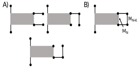
Figure 4: Trees: A) There are 3 ways to extend each tree in ${\cal G}_{N}$ to obtain a tree in ${\cal G}_{N+1}$. B) If a tree in ${\cal G}_{N}$ contains the edge $M_{N}$, then we can obtain another tree in ${\cal G}_{N+1}$ by removing this edge and adding the edges $H_{N+1},B_{N+1}~{}{\rm and}~{}M_{N+1}$

(F1)  A proof of this result is given in [2, 8]. Clearly, $T_{0}=1~{}{\rm and}~{}T_{1}=4$. As shown in Figure 4A, there are 3 ways to extend each tree in ${\cal G}_{N}$ to obtain a tree in ${\cal G}_{N+1}$. If a tree in ${\cal G}_{N}$ contains the edge $M_{N}$, then we can obtain another tree in ${\cal G}_{N+1}$ by removing this edge and adding the edges $H_{N+1},B_{N+1}~{}{\rm and}~{}M_{N+1}$, as shown Figure 4B. It is not hard to show that the number of trees in ${\cal G}_{N}$ that do not contain $M_{N}$ is precisely $T_{N-1}$.

(F2)   This follows from an argument almost identical to that for (F1).

(F3)   If $\beta=H_{k}$ or $B_{k}$, then every path that goes from $N_{in}$ to $N_{out}$ and which passes through $\beta$ must contain the edges $H_{i}~{}{\rm and}~{}B_{i}$ with $i\leq k$ (solid lines in Figure 5A). Every element of ${\cal P}_{N}(\beta)$ is obtained by adding to these edges a tree for the graph with edges $H_{i},B_{i}~{}{\rm and}~{}M_{i}$ with $i\geq k$ (shaded region in Figure 5A). The number of such trees is $T_{N-k}$.

If $\beta=M_{k}$, then every path that goes from $N_{in}$ to $N_{out}$ and which passes through $\beta$ must contain the edges $H_{i}~{}{\rm and}~{}B_{i},i\leq k,$ and $M_{k}$ (solid lines in Figure 5B). Every element of ${\cal P}_{N}(\beta)$ is obtained by adding to these edges a 2-forest for the graph with edges $H_{i},B_{i}~{}{\rm and}~{}M_{i}$ with $i\geq k$. The nodes corresponding to the terminal ends of $\beta$ must be in different trees. The number of such forests is $\sigma_{N-k-1}$.

(F4)   Suppose that $\gamma=H_{j}$. Then every element of $\sigma_{N}(\gamma)$ is of the form ${\cal F}\,\cup\,{\cal T}\,\cup\,B_{j}$ where ${\cal F}$ is any 2-forest for the graph with edges $H_{k},B_{k}~{}{\rm and}~{}M_{k}$ with $k<j$ (blue region in Figure 6A) and ${\cal T}$ is any tree for the graph with edges $H_{k},B_{k}~{}{\rm and}~{}M_{k}$ with $k\geq j$ (grey region in Figure 6A).

If $\gamma=M_{j}$, then consider the graph that does not contain $\gamma$; moreover, $H_{j}\cup H_{j+1}~{}{\rm and}~{}B_{j}\cup B_{j+1}$ are combined into single edges. The number of 2-forests for this graph is $\sigma_{N-1}$. Let ${\cal F}$ be one such forest. If ${\cal F}$ contains both of the combined edges, then it is also an element of $\sigma_{N}(\gamma)$. If ${\cal F}$ does not contain, $H_{j}\cup H_{j+1}$ (or $B_{j}\cup B_{j+1}$) then we obtain an element of $\sigma_{N}(\gamma)$ by adding the edge $H_{j}$ (or $B_{j}$) to ${\cal F}$, as shown in Figure 6C. This demonstrates that the number of forests in $\sigma_{N}(\gamma)$ that contain both $H_{j}~{}{\rm and}~{}B_{j}$ is $\sigma_{N-1}$. To obtain an element of $\sigma_{N}(\gamma)$ that does not contain $H_{j}$ (or $B_{j}$), let ${\cal F}$ be any 2-forest for the graph with edges $H_{k},B_{k}~{}{\rm and}~{}M_{k}$ with $k<j$ (blue region in Figure 6D) and let ${\cal T}$ be any tree for the graph with edges $H_{k},B_{k}~{}{\rm and}~{}M_{k}$ with $k\geq j$ (grey region in Figure 6). Then ${\cal F}\,\cup\,{\cal T}\,\cup\,B_{j}$ (or ${\cal F}\,\cup\,{\cal T}\,\cup\,H_{j})\in\sigma_{N}(\gamma)$.

(F5)   Suppose that $\beta=H_{k}~{}{\rm and}~{}\gamma=M_{j}$. Then every path from $N_{in}$ to $N_{out}$ that passes through $\beta$ must contain the edges $E_{k}=\{H_{i}~{}{\rm and}~{}B_{i}:0\leq i\leq k\}$ (green edges in Figure 7).

If $j<k$, let ${\cal T}$ be any tree in the graph with edges $H_{i},B_{i}~{}{\rm and}~{}M_{n}$ where $k+1\leq i\leq N~{}{\rm and}~{}k\leq n\leq N$ (shaded region in Figure 7A.) There are $T_{N-k}$ such trees and $E_{k}\,\cup\,{\cal F}\in{\cal P}_{N}(\gamma,\beta)$.

If $j=k$, let ${\cal T}$ be any tree in the graph with edges $H_{i},B_{i}~{}{\rm and}~{}M_{i}$ where $k+1\leq i\leq N$. (Shaded region in Figure 7B.) There are $T_{N-k-1}$ such trees and $E_{k}\,\cup\,{\cal F}\in{\cal P}_{N}(\gamma,\beta)$.

If $j>k$, then consider the graph that does not contain $\gamma$ and the edges $M_{i},\,0\leq i<k$. Moreover, $H_{j}\cup H_{j+1}~{}{\rm and}~{}B_{j}\cup B_{j+1}$ are combined into single edges. The number of trees for this graph is $T_{N-k-1}$. Let ${\cal T}$ be one such tree. If ${\cal T}$ contains both of the combined edges, then $E_{k}\cup T$ is an element of ${\cal P}_{N}(\gamma,\beta)$. If ${\cal T}$ does not contain, $H_{j}\cup H_{j+1}$ (or $B_{j}\cup B_{j+1}$) then we obtain an element of ${\cal P}_{N}(\gamma,\beta)$ by adding the edge $H_{j}$ (or $B_{j}$) to ${\cal T}$ and combining this with $E_{k}$. This demonstrates that the number of trees in ${\cal P}_{N}(\gamma,\beta)$ that contain both $H_{j}~{}{\rm and}~{}B_{j}$ is $T_{N-k-1}$. To obtain an element of ${\cal P}_{N}(\gamma,\beta$ that does not contain $H_{j}$ (or $B_{j}$), let ${\cal T}$ be any tree for the graph with edges $H_{i},B_{i}~{}{\rm and}~{}M_{n}$ with $j+1\leq i~{}{\rm and}~{}j\leq n$ (blue region in Figure 7C) and let ${\cal T}_{0}$ be any tree for the graph with edges $H_{i},B_{i}~{}{\rm and}~{}M_{n}$ with $k+1\leq i\leq j-1~{}{\rm and}~{}k\leq n\leq j-1$ (grey region in Figure 7C). Then $E_{k}\cup{\cal T}_{0}\cup{\cal T}\cup B_{j}\cup B_{j+1}\cup H_{j+1}$ (or ${\cal T}\cup{\cal T}_{0}\cup H_{j}\cup H_{j+1}\cup B_{j+1})\in\sigma_{N}(\gamma)$.

(F6)   Suppose that $\beta=H_{k}~{}{\rm and}~{}\gamma=H_{j}$. If $j\leq k$, then there are no paths in ${\cal G}_{N}\backslash\gamma$ from $N_{in}$ to $N_{out}$ that passes through $\beta$. Hence, ${\cal P}_{N}(\gamma,\beta)=0$.

If $j>k$, let $E_{k}$ be the set of edges defined above. Moreover, let ${\cal T}$ be any tree for the graph with edges $H_{i},B_{i},M_{n}$ with $k<i<j~{}{\rm and}~{}k\leq n\ <j$ (grey region in Figure 8B) and ${\cal T}_{0}$ be any tree for the graph with edges $H_{i},B_{i},M_{n}$ with $j+1\leq i\leq N~{}{\rm and}~{}j\leq n\leq N$ (blue region in Figure 8B). Then $E_{k}\cup{\cal T}\cup{\cal T}_{0}\in{\cal P}_{N}(\gamma,\beta)$.

(F7) and (F8)   The derivation is very similar to (F5) and (F6), respectively.

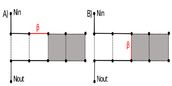
Figure 5: ${\cal P}_{N}(\beta)$

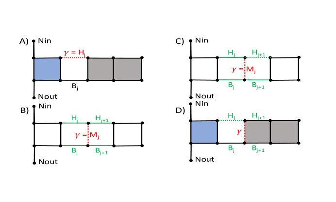
Figure 6: $\sigma_{N}(\gamma)$

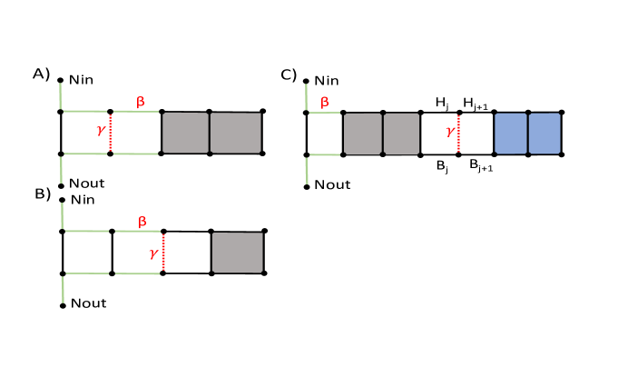
Figure 7: ${\cal P_{N}}(\gamma,\beta),\,\beta=H_{k},\gamma=M_{j}$

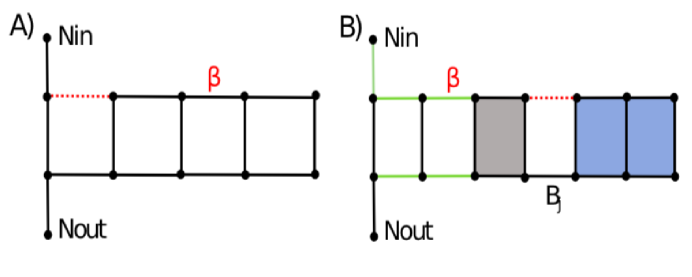
Figure 8: ${\cal P_{N}}(\gamma,\beta),\,\beta=H_{k},\gamma=B_{j}$

References

- [1] W.-K. Chen. Applied Graph Theory. North Holland, 1971.
- [2] M. Desjarlais and R. Molina. Counting spanning trees in grid graphs. Congressus Numerantium, 145:177–185, 2000.
- [3] H. Girouard and C. Iadecola. Neurovascular coupling in the normal brain and in hypertension, stroke, and alzheimer disease. J Appl Physiol, 100(1):328–35, 2006.
- [4] C. Iadecola. Neurovascular regulation in the normal brain and in alzheimer’s disease. Nat Rev Neurosci, 5(5):347–60, 2004.
- [5] S. N. Jespersen and L. Ostergaard. The roles of cerebral blood flow, capillary transit time heterogeneity, and oxygen tension in brain oxygenation and metabolism. J Cereb Blood Flow Metab, 32(2):264–77, 2012.
- [6] L. Ostergaard and T. S. Engedal et. al. Capillary transit time heterogeneity and flow-metabolism coupling after traumatic brain injury. J Cereb Blood Flow Metab, 34(10):1585–98, 2014.
- [7] L. Ostergaard, S. B. Kristiansen, H. Angleys, J. Frokiaer, J. M. Hasenkam, S. N. Jespersen, and H. E. Botker. The role of capillary transit time heterogeneity in myocardial oxygenation and ischemic heart disease. Basic Res Cardiol, 109(3):409, 2014.
- [8] P. Raff. Spanning trees in grid graphs. arXiv:0809.2551, 2008.
- [9] D. Terman, L. Chen, and Y. Hannawi. Mathematical modeling of cerebral capillary blood flow heterogeneity and its effect on brain tissue oxygen. Submitted, 2020.