Euclidean wormhole in the SYK model

Abstract

We study a two-site Sachdev-Ye-Kitaev (SYK) model with complex couplings, and identify a low temperature transition to a gapped phase characterized by a constant in temperature free energy. This transition is observed without introducing a coupling between the two sites, and only appears after ensemble average over the complex couplings. We propose a gravity interpretation of these results by constructing an explicit solution of Jackiw-Teitelboim (JT) gravity with matter: a two-dimensional Euclidean wormhole whose geometry is the double trumpet. This solution is sustained by imaginary sources for a marginal operator, without the need of a coupling between the two boundaries. As the temperature is decreased, there is a transition from a disconnected phase with two black holes to the connected wormhole phase, in qualitative agreement with the SYK observation. The expectation value of the marginal operator is an order parameter for this transition. This illustrates in a concrete setup how a Euclidean wormhole can arise from an average over field theory couplings.

I Introduction

Wormholes are geometric shortcuts that connect distant points in spacetime. Their role in the Euclidean path integral has been hotly debated in the literature Lavrelashvili et al. (1987); Hawking (1987); Giddings and Strominger (1988a, b, 1989); Coleman (1988); Maldacena and Maoz (2004); Arkani-Hamed et al. (2007); Hertog et al. (2019); Hebecker et al. (2018). In the context of holography, an important puzzle is that geometries connecting two boundaries indicate that the partition function of the dual field theory does not factorize Maldacena and Maoz (2004). To address this problem, one could simply decide not to include these configurations. However, it has been recently realized that it is only after including Euclidean wormholes that one gets results consistent with the interpretation of black holes as ordinary quantum systems. This has been shown explicitly in Jackiw-Teitelboim gravity Jackiw (1985); Teitelboim (1983), a two-dimensional theory of gravity capturing the low-energy dynamics of near-extreme black holes Jensen (2016); Maldacena et al. (2016); Engelsöy et al. (2016), for the spectral form factor Saad et al. (2018, 2019), for correlations functions Saad (2019), and for the fine-grained entropy of evaporating black holes Penington (2020); Almheiri et al. (2019); Penington et al. (2020); Almheiri et al. (2020a, b). The factorization puzzle suggests that the gravitational path integral requires some form of ensemble averaging, whose origin remains mysterious. We refer to Blommaert et al. (2019); Betzios et al. (2019); Marolf and Maxfield (2020); Pollack et al. (2020); Raamsdonk (2020); Betzios and Papadoulaki (2020); Giddings and Turiaci (2020); Blommaert (2020); Anous et al. (2020); Chen et al. (2020); Eberhardt (2020); Stanford (2020); McNamara and Vafa (2020); Alishahiha et al. (2020); Cotler and Jensen (2020a) for recent discussions on this issue.

This problem doesn’t arise in Lorentzian signature because non-traversable wormholes have horizons, which make them consistent with the factorization of the field theory dual. In this case, wormholes are interpreted as coming from quantum entanglement Maldacena (2003); Maldacena and Susskind (2013). It has also been recently shown that these wormholes can be rendered traversable by introducing a double trace coupling between the boundaries Gao et al. (2017); Maldacena et al. (2017). In particular, Maldacena and Qi Maldacena and Qi (2018), see also Bak et al. (2018); Kim et al. (2019), have described an eternal traversable wormhole solution in JT gravity with a double trace deformation, and argued that a dual picture consists in two copies of a Sachdev-Ye-Kitaev (SYK) model French and Wong (1970); Bohigas and Flores (1971); Sachdev and Ye (1993); Kitaev ; Maldacena and Stanford (2016); Jensen (2016); Jevicki et al. (2016); García-García and Verbaarschot (2016, 2017); Bagrets et al. (2016, 2017) weakly coupled by a one-body operator. The system undergoes a first order transition at finite temperature from the wormhole to a two black holes phase which can also be characterized by spectral statistics García-García et al. (2019).

In this paper, we propose a Euclidean version of this story which doesn’t involve an explicit coupling between the boundaries. In section II, we show that the free energy of a two-site SYK model with complex couplings, obtained by exact diagonalization of the Hamiltonian, undergoes a low temperature transition to a gapped phase similar to that of the wormhole of Maldacena and Qi (2018), and which arises only after an ensemble average over couplings. In section III, we describe a Euclidean wormhole solution of JT gravity plus matter, which does not require a coupling between the two boundaries, but is instead sustained by imaginary sources. We compute the free energy and show that this system undergoes a similar phase transition from a high temperature phase with two black holes to a low temperature wormhole phase, in qualitative agreement with the SYK behavior. We end with a discussion and conclusions in section IV.

II Sachdev-Ye-Kitaev with complex couplings

We study two uncoupled non-Hermitian SYK models with complex couplings composed by $N$ Majorana fermions in $(0+1)$ dimensions with infinite range interactions in Fock space. One of the copies is called Left ($L$) with Majoranas denoted $\psi_{L}$. The other copy is called Right ($R$) with Majoranas denoted $\psi_{R}$. Majoranas in each copy are governed by an SYK Hamiltonian with complex couplings with the left Hamiltonian being the complex conjugate of the right one:

$$H_{L}\, =\,\frac{1}{4!}\sum_{i,j,k,l=1}^{N/2}(J_{ijkl}+i\kappa M_{ijkl})\,\psi_{L,i}\,\psi_{L,j}\,\psi_{L,k}\,\psi_{L,l}\,$$

$$H_{R}\, =\,\frac{1}{4!}\sum_{i,j,k,l=1}^{N/2}(J_{ijkl}-i\kappa M_{ijkl})\,\psi_{R,i}\,\psi_{R,j}\,\psi_{R,k}\,\psi_{R,l}$$ (1)

where $\kappa$ is a real positive number, $\{\psi_{A,i},\psi_{B,j}\}=\delta_{AB}\delta_{ij}$ $(A,B=L,R)$ and $J_{ijkl},M_{ijkl}$ are Gaussian distributed random variables with zero average and standard deviation $\sqrt{\langle J_{ijkl}^{2}\rangle}=\sqrt{\langle M_{ijkl}^{2}\rangle}=4\sqrt{6}/{N^{3/2}}$, see Kitaev ; Maldacena and Stanford (2016). We note that both Hamiltonians are non-Hermitian and there is no explicit coupling between them.

The combined system Hamiltonian

$$H=H_{L}+H_{R}$$ (2)

has a complex spectrum with complex conjugation symmetry: if $E_{n}$ is an eigenvalue, its complex conjugate $E_{n}^{\ast}$ is also an eigenvalue. We shall see that despite the fact that the two copies are decoupled, the combined system after ensemble average shares many of the properties expected from a Euclidean wormhole.

We compute the spectrum by exact diagonalization techniques with $N\leq 34$. The spectrum for a single disorder realization is depicted in Fig. 1 for different values of $\kappa$ which is the only free parameter of the model. For $\kappa=1$, the eigenvalues are distributed in the complex plane with an ellipsoid shape with axis of similar sizes. Not surprisingly, for small $\kappa=0.1$, although the spectrum still has an ellipsoid shape, it is mostly concentrated close to the real axis. More information is revealed, see lower plots in Fig. 1, in the spectral density of the real and imaginary parts of the eigenvalues after $1000$ disorder realizations. The spectral density of the real part seems to be qualitatively similar to that of the SYK model with real couplings. The imaginary part shows by contrast a sharp peak at zero and a relatively small depression around zero energy. A similar peak is observed for other values of $\kappa$, though its strength, as expected, diminishes as $\kappa$ increases. We do not have a clear understanding of why some eigenvalues have zero imaginary part even in the bulk of the spectrum while there is some level repulsion around zero. The latter is likely related to conjugation symmetry of the spectrum that effectively acts as a chiral symmetry inducing level repulsion around states with zero (imaginary) energy. Real eigenvalues are not beneficial for the establishment of the wormhole phase because the absence of an imaginary part prevents the cancellations necessary for its existence. Likely, this is not important as the mentioned cancellations only occur in the infrared limit of the spectrum where the number of real eigenvalues, other than the ground state, is small. An important feature of the spectrum is that the ground state $E_{0}$ is always real for any $\kappa$ or strength of disorder.

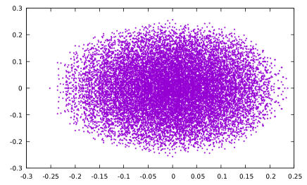
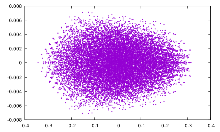
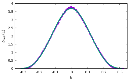
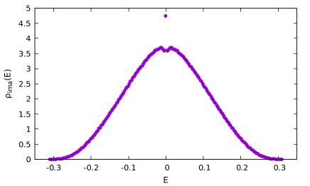
Figure 1: Top: Complex spectrum of the combined Hamiltonian (2) for $N=30$ and, $\kappa=1$ (left) and $\kappa=0.1$ (right). Note the different scale of each figure. Bottom: Spectral density of the real (left) and imaginary (right) part of the eigenvalues for $\kappa=1$, $N=34$ after average over $45$ disorder realizations. The real part looks qualitatively similar to that of a single SYK model with real couplings. Indeed, it agrees well (solid line) with the analytical prediction, see $(24)$ of García-García and Verbaarschot (2017), valid everywhere except in the tail of the spectrum. The best fitting is close to the analytical prediction for $2N$ Majoranas. Regarding the imaginary part, it is characterized by a peak at zero energy followed by a suppression for small energies whose origin at present we do not understand well.

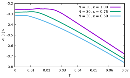
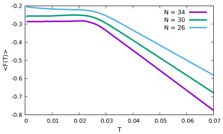
Figure 2: Left: Free energy after ensemble average of $300$ disorder realizations for $N=30$ Majoranas and different strengths of the imaginary part $\kappa$. Right: Free energy for $\kappa=1$ and different $N$’s.

We can now proceed to the calculation of the thermodynamic properties. Interestingly, because complex conjugation is a symmetry of the spectrum, the partition function of the combined system $Z(\beta)=\textrm{Tr}\,e^{-\beta H}$ is real. In order to reduce statistical fluctuations, we carry out an ensemble average and compute the resulting quenched free energy:

$$\left\langle F(T)\right\rangle=-T\left\langle{\log Z(\beta)}\right\rangle,$$ (3)

where $\beta=1/T$. Results depicted in Fig. 2 for different values of $\kappa$ show a surprising result. The free energy is constant for sufficiently low $T$ and there is a rather abrupt change at a certain critical temperature that suggests the existence of a first order transition. We note that a sharp transition only occurs in the $N\to\infty$ limit. Although numerically it is hard to reach beyond a comparatively small value of $N\sim 34$, it is still important to assess the magnitude of finite $N$ effects in the range of available sizes. Results depicted in the right plot of Fig. 2 show that these effects are relatively small, consistent already with $1/N$ corrections. As is expected, these perturbative finite $N$ effects tend to increase the free energy.

Roughly speaking, the location of the kink, which corresponds to the critical temperature, seems to scale approximately as $\kappa^{2}$. A precise determination is difficult because for small $\kappa\ll 1$ it becomes harder to clearly see the low temperature phase. This could be a finite $N$ effect or might signal the existence of a minimum value of $\kappa$, even in the large $N$ limit, for a gap to be formed. For large $\kappa\gg 1$, the free energy is initially constant but display modulations (not shown) at intermediate temperatures. At present, we do not have an explanation for this intermediate phase. We can only say that it does not seem to be a statistical fluctuation that will go away in the large $N$ limit or if more disorder realizations are considered.

This free energy is very similar to both the free energy of the eternal traversable wormhole studied in Maldacena and Qi (2018) and to that of the Euclidean wormhole described in the next section. A constant free energy signals the existence of a gap in the spectrum that separates the ground state from higher excitations of the system. The existence of the gap can be explained by the combined effect of a complex spectrum, the mentioned complex conjugation symmetry, and ensemble average as follows.

Writing the spectrum of $H$ as, $E_{n}=a_{n}+ib_{n}$ where $a,b$ are real numbers, using the fact that if $E_{n}$ is an eigenvalue then $E_{n}^{*}$ is also an eigenvalue and that the ground state $E_{0}$ is real, we write the partition function for a given disorder realization as, $Z(\beta)=e^{-\beta E_{0}}+2\sum_{n}\mathrm{cos}(\beta b_{n})\,e^{-\beta a_{n}}$, assuming no degeneracies. After ensemble average, the free energy becomes

$$\langle\beta F\rangle=-\left\langle{\log(e^{-\beta E_{0}}+2\sum_{n}\mathrm{cos}(\beta b_{n})\,e^{-\beta a_{n}})}\right\rangle.$$ (4)

Figure 3: Dependence of free energy of the Hamiltonian (2) on the number of disorder realizations $N_{dis}$ for $N=30$ and $\kappa=1$. A flat free energy in the low temperature limit that signals a gapped spectrum and a wormhole phase is only observed after ensemble average with a large number of disorder realizations.

In the high temperature limit $\beta\to 0$, the argument of the cosine function is always small and $\mathrm{cos}\sim 1$. As a consequence, the imaginary part of the spectrum becomes effectively irrelevant and the spectrum corresponds to that of two identical, uncoupled, systems, in this case two SYK models with real couplings. Assuming that a gravity dual picture still applies, this region corresponds to a phase with two black holes.

In the opposite limit $\beta\to\infty$, corresponding to low temperatures, the cosine becomes a highly oscillating function whose features depend on the form of the imaginary part of the spectrum. From the results depicted in Fig. 1, the imaginary part of the spectrum seems to vary greatly, especially for intermediate $\kappa$, even for eigenvalues close to the ground state. In any case, the variations of the imaginary part are much faster than those of the real part.

The effect of the ensemble average is to effectively suppress the contribution of eigenvalues in the lower part of the spectrum, allowing the opening of a gap above the ground state $E_{0}$. This leads to a free energy very similar to the one recently reported for the eternal traversable wormhole Maldacena and Qi (2018). The main differences is that in our setup, there is no explicit coupling between the two copies.

We now address in more detail the importance of ensemble average in our results. In Fig. 3, we depict results for the free energy after ensemble average with an increasing number of disorder realizations. For a small number of disorder realizations, the free energy in the low temperature limit is far from being flat. Peaks and oscillations of different frequencies are observed. Only after performing the average with a comparatively large number of realizations, the free energy becomes completely flat in this limit which is a signature of a gapped spectrum and a wormhole. It could be argued that, for a much larger number of Majoranas, which for $N\geq 36$ is numerically expensive, spectral average on a single realization of disorder is enough to flatten the free energy but at present we do not have evidence of this. Moreover, even if we could reach a much larger value of $N$, we believe that if no ensemble average is carried out, it would be necessary to perform a spectral average in a small window to smooth out fluctuations.

In the next section, we will see that the free energy of our SYK setup is strikingly similar to that of a solution of JT gravity plus matter, a Euclidean wormhole with the geometry of the double trumpet. This led us to propose that the low-temperature phase that we observe in our SYK setup should be interpreted as a Euclidean wormhole. Therefore, with the present evidence, ensemble average in the field theory dual is a crucial ingredient to reproduce the expected features of a Euclidean wormhole, as expected from factorization arguments. Finally, let us comment on the advantage of exact diagonalization techniques with respect to the solution of Schwinger-Dyson equations in the large $N$ limit. There, the ensemble average is carried out earlier in the derivation of the equations and therefore it is not possible to determine its exact role in observing the gap at low temperature. In contrast, exact diagonalization displays without ambiguity the central role played by the ensemble average.

III The double trumpet solution

We have observed that the SYK model with complex couplings has a low temperature phase which behaves like a wormhole. In this section, we propose a gravitational interpretation of this phase, as a novel Euclidean wormhole solution of JT gravity plus matter, where the crucial ingredient is the introduction of imaginary sources for a marginal operator.

The theory we consider is JT gravity with a massless scalar field, described by the action

$$S=S_{\mathrm{JT}}+S_{\mathrm{matter}}~{},$$ (5)

where we have

$$S_{\mathrm{JT}} = -{S_{0}\over 2\pi}\left[{1\over 2}\int d^{2}x\sqrt{g}\,R+\int d\tau\sqrt{h}\,K\right]-{1\over 2}\int d^{2}x\sqrt{g}\,\Phi(R+2)-\int d\tau\sqrt{h}\,\Phi(K-1)~{},$$ (6)

$$S_{\mathrm{matter}} = {1\over 2}\int d^{2}x\sqrt{g}\,(\partial\chi)^{2}~{}.$$ (7)

JT gravity is a two-dimensional theory that captures the low-energy dynamics of higher-dimensional near-extreme black holes Almheiri and Polchinski (2015); Maldacena et al. (2016); Almheiri and Kang (2016); Nayak et al. (2018); Castro and Godet (2020). The parameter $S_{0}$ is interpreted as the extremal entropy and is taken to be large. In the Euclidean path integral Saad et al. (2019), the first term in (6) gives the topological contribution $e^{-S_{0}(2g+n-2)}$ to a geometry of genus $g$ with $n$ boundaries, so a large value of $S_{0}$ suppresses higher genus contributions.

The solution we will describe has the geometry of the double trumpet: a Euclidean geometry with $R=-2$ and with two asymptotic boundaries. It can be described by the metric

$$ds^{2}={1\over\mathrm{cos}^{2}\rho}\left(d\tau^{2}+d\rho^{2}\right)~{},\qquad-{\pi\over 2}\leq\rho\leq{\pi\over 2}~{},\qquad\tau\sim\tau+b~{},$$ (8)

which is just global AdS₂ with periodically identified Euclidean time. The proper length of the geodesic at $\rho=0$ is called $b$ and is the only parameter of the geometry. In JT gravity, we also have a left and right inverse temperatures $\beta_{L}$ and $\beta_{R}$, defined as the periods of the respective boundary times, see Fig. 4.

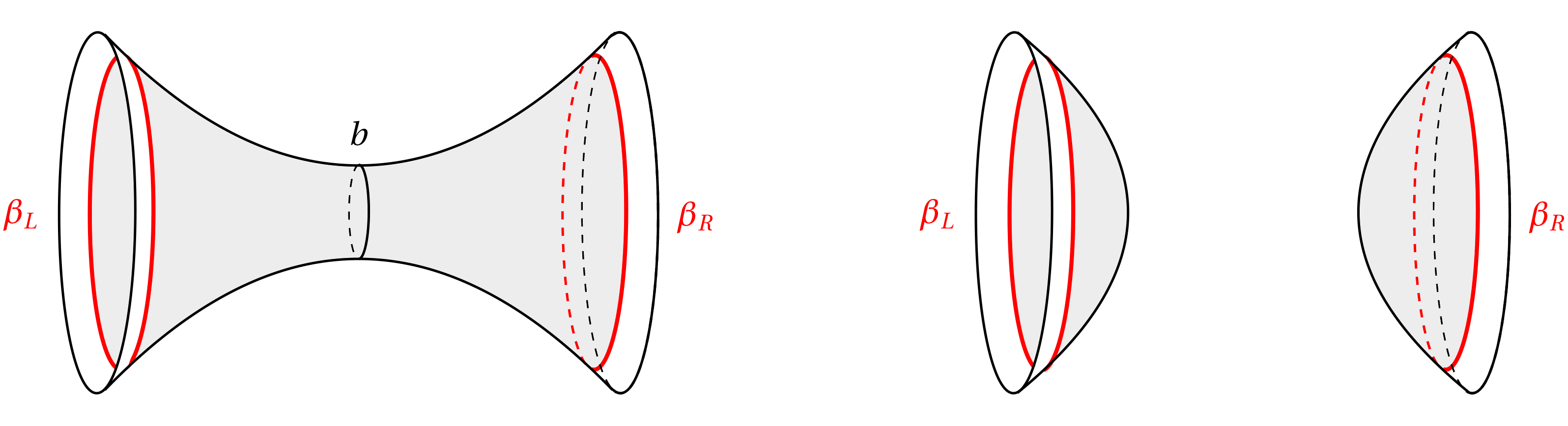
Figure 4: Left: Double trumpet geometry corresponding to the wormhole phase. Right: Hyperbolic disks corresponding to the disconnected phase with two black holes. We observe a low temperature transition between these two phases.

The double trumpet geometry is not an ordinary solution of JT gravity plus matter. The crucial additional ingredient that we use here is to turn on imaginary sources for a massless scalar field. The motivation for this comes from the SYK story described in the previous section. There, a wormhole-like phase appears after adding an imaginary part to the couplings. We can interpret that as a deformation of the left and right Hamiltonian by an operator

$$\delta H_{L}=-i\kappa M_{L},\qquad\delta H_{R}=i\kappa M_{R}~{},\qquad M\equiv\frac{1}{4!}\sum_{i,j,k,l=1}^{N/2}M_{ijkl}\,\psi_{i}\,\psi_{j}\,\psi_{k}\,\psi_{l}~{}.$$ (9)

We aim to investigate the effect of a qualitatively similar deformation on the gravity side. For that purpose, we deform the JT gravity action by a scalar operator $\mathcal{O}$ on each side

$$\delta S=-ik\int_{S^{1}_{L}}d\tau\,\mathcal{O}_{R}(\tau)+ik\int_{S^{1}_{R}}d\tau\,\mathcal{O}_{L}(\tau)~{},$$ (10)

where the source is $ik$ on the left boundary and $-ik$ on the right boundary. Using the standard AdS/CFT dictionary, this should correspond to fixing the asymptotic value of some bulk scalar field $\chi$.

To obtain a wormhole solution in JT with matter, it turns out that we should take $\mathcal{O}$ to have conformal dimension $\Delta=1$ so that $\chi$ is a massless scalar field in the bulk. This is explained in Appendix B. The condition we impose is then

$$\lim_{\rho\rightarrow{\pi/2}}\chi=ik,\qquad\lim_{\rho\to-{\pi/2}}\chi=-ik~{},$$ (11)

and we will see that this makes the wormhole solution possible. To be clear, we are not claiming that this follows from a precise holographic duality. It must be understood as a setup in Euclidean JT gravity plus matter, which is inspired by the previous SYK results, and turns out to provide a qualitatively similar picture in gravity. The parameter $k$ in gravity is analogous to $\kappa$ in SYK but we do not aim to establish a precise quantitative correspondence between the two.

III.1 Equations of motion

Let us now solve the equations of motion. The scalar field $\chi$ satisfies the massless wave equation

$$\Box\chi=0~{}.$$ (12)

Together with the condition (11) coming from the imaginary sources, this fixes the classical solution to be

$$\chi={2ik\over\pi}\rho~{}.$$ (13)

We are finding here an imaginary solution for a real scalar field $\chi$ because of the complex sources. In Lorentzian signature, imaginary sources are unphysical as they lead to violations of the averaged null energy condition. Indeed, they can be used to construct traversable wormholes in AdS without a non-local coupling between the boundaries, in contradiction with the “no-transmission principle” Engelhardt and Horowitz (2016) (see Freivogel et al. (2019) for a related discussion). In Euclidean signature, these imaginary sources do make sense. They can be defined by analytic continuation from real sources in the thermal partition function and can be used to study the statistical mechanics of a physical system. For example, imaginary chemical potentials have been useful in studying the phase diagram of gauge theories Roberge and Weiss (1986); de Forcrand and Philipsen (2002).

We now impose the equation of motion for the JT dilaton which is

$$\nabla_{\mu}\nabla_{\nu}\Phi-g_{\mu\nu}\Box\Phi+g_{\mu\nu}\Phi+\langle T_{\mu\nu}^{\chi}\rangle=0~{}.$$ (14)

The stress tensor of $\chi$ decomposes into a classical and a quantum piece

$$\langle T_{\mu\nu}^{\chi}\rangle=T_{\mu\nu}^{\mathrm{class}}+T_{\mu\nu}^{\mathrm{quantum}}~{}.$$ (15)

The classical piece is obtained by evaluating $T_{\mu\nu}$ on the solution (13), which leads to

$$T_{\mu\nu}^{\mathrm{class}}=\partial_{\mu}\chi\partial_{\nu}\chi-{1\over 2}g_{\mu\nu}(\partial\chi)^{2}={2k^{2}\over\pi^{2}}\begin{pmatrix}1&0\\ 0&-1\end{pmatrix}~{}.$$ (16)

This generates negative energy in the bulk because the solution for $\chi$ is pure imaginary. What would normally be positive energy for real sources becomes negative energy for imaginary sources.

In addition to this classical piece, there is also a quantum stress tensor due to the Casimir energy of $\chi$. Although this piece is negligible in the regime where we will compare with the previous field theory results, it becomes important at higher temperature, where it destabilizes the wormhole. The quantum stress tensor can be computed explicitly, using the Green function method and point splitting, as detailed in Appendix A. The result is

$$T_{\mu\nu}^{\mathrm{quantum}}=-{1\over 24\pi}g_{\mu\nu}-{\mathcal{E}(b)\over\pi}\begin{pmatrix}1&0\\ 0&-1\end{pmatrix}~{},$$ (17)

where we have introduced the quantity

$$\mathcal{E}(b)\equiv\sum_{n\geq 1}{1\over 4\,\mathrm{sinh}^{2}({nb\over 2})}>0~{},$$ (18)

whose properties are given in the Appendix A.

We can now solve for the JT dilaton using (14). The general solution is given by

$$\Phi=\left({2k^{2}\over\pi}-\mathcal{E}(b)\right)(1+\rho\,\mathrm{tan}\,\rho)+{\eta\over 2}\,\mathrm{tan}\,\rho+{1\over 24\pi}~{},$$ (19)

where $\eta$ is an arbitrary constant. The existence of the wormhole requires that $\Phi\to+\infty$ at both boundaries. Expanding this solution at the two boundaries gives

$$\Phi \underset{\rho\to+{\pi\over 2}}{\sim} \left({k^{2}\over\pi}-{\mathcal{E}(b)\over 2}+{\eta\over 2}\right){1\over{\pi\over 2}-\rho}+\dots~{},$$ (20)

$$\Phi \underset{\rho\to-{\pi\over 2}}{\sim} \left({k^{2}\over\pi}-{\mathcal{E}(b)\over 2}-{\eta\over 2}\right){1\over{\pi\over 2}+\rho}+\dots~{}.$$ (21)

The position of the left and right boundaries are determined by imposing the boundary condition $\Phi=\bar{\phi}_{r}/\epsilon$. We should also impose the boundary conditions for the metric

$$ds^{2}\underset{\rho\to{\pi\over 2}}{\sim}{du_{R}^{2}\over\epsilon^{2}},\qquad ds^{2}\underset{\rho\to-{\pi\over 2}}{\sim}{du_{L}^{2}\over\epsilon^{2}}~{},$$ (22)

which tell us how $u_{L}$ and $u_{R}$ are related to $\tau$. The left and right temperatures are defined as their periods $u_{L}\sim u_{L}+\bar{\phi}_{r}\beta_{L},u_{R}\sim u_{R}+\bar{\phi}_{r}\beta_{R}$ rescaled by $\bar{\phi}_{r}$ for convenience. This gives

$$\beta_{L}={2b\over{2k^{2}\over\pi}-\,\mathcal{E}(b)-\eta},\qquad\beta_{R}={2b\over{2k^{2}\over\pi}-\,\mathcal{E}(b)+\eta}~{}.$$ (23)

We see that $b$ and $\eta$ are determined by the boundary conditions: they are fixed by the choice of temperatures on each side. The condition for the existence of the wormhole is that $\beta_{L},\beta_{R}\geq 0$. In the following, we will set the asymmetry parameter $\eta$ to zero so that we consider a situation where $\beta_{L}=\beta_{R}$.

The temperature $T=T_{L}=T_{R}$ is then

$$T={k^{2}\over\pi b}-{\,\mathcal{E}(b)\over 2b}~{}.$$ (24)

At large $b$, this is positive since we have $\mathcal{E}(b)\sim e^{-b}$ which becomes negligible. Hence, this gives a consistent wormhole solution. From the expression of the temperature, we see that the existence of the solution depends crucially on the pure imaginary sources. Real sources would change the sign of $k^{2}$ and prevent the solution to exist. Moreover, we see that the Casimir energy contributes negatively (since $\mathcal{E}(b)>0$) indicating that it has a destabilizing effect which is described in more detailed below.

It’s interesting to note that the operator $\mathcal{O}$ acquires an imaginary expectation value

$$\langle\mathcal{O}_{L}\rangle={2ik\over\pi}~{},\qquad\langle\mathcal{O}_{R}\rangle=-{2ik\over\pi}~{},$$ (25)

which can be read off from the solution for $\chi$ using the AdS/CFT dictionary. This is a consequence of the imaginary gradient in the solution for $\chi$. We will see below that this expectation value is an order parameter for the phase transition.

It’s interesting to note that the marginality of the operator $\mathcal{O}$ is important for the wormhole solution to be possible. Indeed, an operator $\mathcal{O}$ with $\Delta\neq 1$ doesn’t lead to a consistent solution because it makes the dilaton grow too fast or too slow, see Appendix B.

III.2 Thermodynamics

We now compute the free energy of the wormhole solution. The partition function is

$$\log Z = -b^{2}T+{2bk^{2}\over\pi}+\log\textrm{Tr}\,e^{-bL_{0}}~{}.$$ (26)

The first term comes from the classical contribution of the Schwarzian action that describes the two trumpet geometries Saad et al. (2019) in conventions where $8\pi G_{N}=1$. The corresponding one-loop term proportional to $\log T$ is always negligible in our discussion and will be ignored. The second term is the on-shell action of the classical matter solution (13). The third term is the one-loop contribution from the matter, which can be derived as follows. The path integral of the scalar field $\chi$ on a cylinder of width $\pi$ and circumference $b$ gives the thermal partition function

$$Z_{\mathrm{cylinder}}^{\chi}=\textrm{Tr}\,e^{-b\left(L_{0}-{1\over 24}\right)}={1\over\eta(e^{-b})}~{},$$ (27)

where $\eta(q)$ is the Dedekind eta function. We can perform a Weyl transformation to the double trumpet. It follows from the discussion in Maldacena and Qi (2018) that the effect of the Weyl anomaly is to shift the ground state energy by removing the $-{1\over 24}$, so we end up with

$$Z^{\chi}=\textrm{Tr}\,e^{-bL_{0}}={e^{-b/24}\over\eta(e^{-b})}~{}.$$ (28)

This formula is also a consequence of the computation of the quantum stress tensor in Appendix A.

The saddle point of (26) with respect to $b$ leads to the relation

$$T={k^{2}\over\pi b}-{\mathcal{E}(b)\over 2b}~{},$$ (29)

where we used that $\mathcal{E}(b)={1\over 24}+\partial_{b}\log\eta(e^{-b})$ from the identities given in Appendix A. Note that $\mathcal{E}(b)=\langle L_{0}\rangle_{b}$ is the thermal expectation value of $L_{0}$ at the inverse temperature $b$. It is a nice consistency check that this expression of $T$ matches with (24) obtained from the explicit solution.

Large wormhole regime.

Let’s first consider a regime where $b$ is large. In this regime, we have $\mathcal{E}(b)\sim e^{-b}$ so the second term of (29) becomes negligible as soon as $b$ becomes relatively large. We then have the saddle point $b_{\ast}={k^{2}\over\pi T}$ which leads to the free energy

$$F_{\mathrm{WH}}=-T\log Z=-{k^{4}\over\pi^{2}}~{},\qquad\text{when }\quad\mathcal{E}(b_{\ast})\ll k^{2}$$ (30)

This formula is valid when $\mathcal{E}\left({k^{2}\over\pi T}\right)\ll k^{2}$ which holds at sufficiently low temperature since we have $\mathcal{E}\left({k^{2}\over\pi T}\right)\sim_{T\to 0}e^{-k^{2}/(\pi T)}$. We see that the wormhole has constant negative free energy at low temperature, as is expected from a gapped system. This is the regime where we expect that JT gravity and the SYK model share similar features.

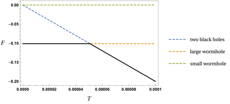
Figure 5: Plot of the free energy of the wormhole and the black holes at low temperature. The solid black line represents the free energy of the system. It corresponds with that of the wormhole, characterized by a constant negative free energy, at sufficiently low (high) temperatures. As temperature increases, we observe a first order transition separating the wormhole from the two black hole phase. This qualitatively matches the behavior seen in the SYK with complex couplings. Notice that there is also another solution at smaller $b$ whose free energy is always larger. We use $k=1$ and $S_{0}=10^{3}$.

Our gravitational boundary conditions consist of two circles of length $\beta=1/T$ and Dirichlet boundary conditions for the scalar field $\chi$ given in (11). Besides the double trumpet solution, we can also have two disconnected black holes (i.e. two hyperbolic disks). In a black hole, the source for the scalar field doesn’t contribute to the on-shell action, because the classical solution is just $\chi=\mathrm{const}$. The one-loop contribution gives a contribution that depends on $\epsilon$ and gets renormalized away. As a result, the free energy of the two black holes is the same as in pure JT gravity:

$$F_{\mathrm{BH}}=-T\log Z=-2S_{0}T-4\pi^{2}T^{2}~{}.$$ (31)

The physical free energy is then the minimum

$$F=\min\left(F_{\mathrm{WH}},F_{\mathrm{BH}}\right)~{},$$ (32)

and there is a phase transition at the critical temperature

$$T_{c}\underset{k^{2}\ll S_{0}}{\sim}{k^{4}\over 2\pi^{2}S_{0}}~{}.$$ (33)

The classical solution $\chi=\mathrm{const}$ in the black hole phase implies that the expectation value of the marginal operator vanishes:

$$\langle\mathcal{O}_{L}\rangle=0~{},\qquad\langle\mathcal{O}_{R}\rangle=0~{},$$ (34)

This shows that the expectation value of $\mathcal{O}$ is an order parameter for the transition from the two black holes to the wormhole. It is zero in the black hole phase, and becomes non-zero in the wormhole phase, where we have (25). The non-zero expectation value at one boundary is a direct consequence of the source at the other boundary so this can be seen as a field theory incarnation of the geometric connection in the bulk.

Comparison with SYK.

The above computation gives the annealed free energy $-T\log\,\langle Z\rangle$ where the ensemble average $\langle\,\cdot\,\rangle$ is defined by the Euclidean path integral. To compare with the SYK setup, we should instead compute the quenched free energy $-T\langle\log Z\rangle$. It was recently explained Engelhardt et al. (2020) that the quenched free energy can be computed in gravity by including corrections from replica wormholes. These corrections are computed below in the next section III.3 and shown to give a negligible correction in the low temperature regime. This allows us to compare the gravitational free energy plotted in Fig. 5 to the SYK free energy shown in Fig. 2. The qualitative agreement of the free energies supports our proposal that the low-temperature phase observed in our SYK setup should be interpreted as a Euclidean wormhole.

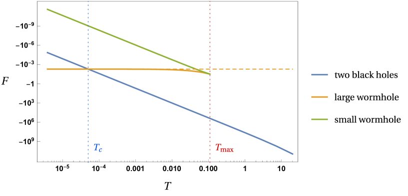
Figure 6: Log-log plot of the free energy of the different solutions. We plot the disconnected contribution of the two black holes (in blue). It dominates at high temperature until the phase transition at $T=T_{c}$ (dashed vertical blue line) after which the large wormhole solution (in orange) becomes favorable. There is also a small wormhole solution (in green) which has higher free energy. Both wormhole solutions only exist below a maximal temperature $T_{\mathrm{max}}$ (dashed vertical red line) and we have $T_{\mathrm{max}}>T_{c}$. The dashed orange line corresponds to the classical approximation where we don’t include the Casimir energy of the matter, thus obtaining a wormhole at all temperatures. This shows that the Casimir energy has a destabilizing effect which is responsible for the existence of both the maximal temperature and the small wormhole solution.

General analysis.

Let’s now analyze the solution more generally, beyond the regimes where JT gravity is well approximated by SYK. Firstly, the wormhole solution only exists if $T\geq 0$. Since $\mathcal{E}(b)$ is a decreasing function of $b$, we see that this implies that there is a minimal value of $b$ defined implicitly by

$$\mathcal{E}(b_{\mathrm{min}})={2k^{2}\over\pi}~{}.$$ (35)

The formula (29) also implies that there is a maximal value $T_{\mathrm{max}}$ of the temperature beyond which the wormhole solution disappears. This value is attained when $\partial_{b}T=0$ and the solution only exists when $0\leq T\leq T_{\mathrm{max}}$. In this range, there are actually two values of $b$ that give the same $T$: the large wormhole that was discussed previously but also a small wormhole at a much smaller value of $b$. This is the result of a competition between the classical negative energy coming from the imaginary sources, and the positive quantum Casimir energy of the matter. It is here a classical effect that sustains the wormhole while a quantum effect destabilizes it. It can be checked that the smaller wormhole has always higher free energy than the large one, so that it never dominates in the canonical ensemble. The main thermodynamic features of the system are summarized in Fig. 6 which describes the free energy of the different branches as a function of temperature and Fig. 7 that depicts the dependence of the wormhole size $b$ with temperature.

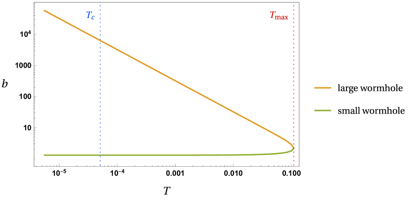
Figure 7: Log-log plot of the size $b$ of the wormhole as a function of the temperature. We use $k=1$ and $S_{0}=10^{3}$.

III.3 Quenched versus annealed in gravity

As pointed out in Engelhardt et al. (2020), the gravitational free energy must be computed with a replica trick because we are interested in the quenched, rather than annealed, free energy. This means that the naive answer for the free energy (i.e. the annealed one) might be incorrect in situations where quantum gravity effects are important. For a system with boundary $B$, we should compute the gravitational path integral $\mathcal{P}(B^{m})$ whose boundary is $m$ copies of $B$, analytically continue in $m$ and use the formula

$$\langle\log Z(B)\rangle=\lim_{m\to 0}{1\over m}(\mathcal{P}(B^{m})-1)~{}.$$ (36)

We take $B$ to be the system with two circle boundaries: one is labeled $+$ and has a source $+ik$ while the other is labeled $-$ and has the source $-ik$. The wormhole solution can only connect a $+$ circle to a $-$ circle. We take the temperature to be not too small so that taking $S_{0}$ to be large allows us to ignore the higher genus topologies. A typical contribution to $\mathcal{P}(B^{m})$ is drawn in Fig. 8.

Denoting by $Z_{1}$ the black hole contribution and by $Z_{2}$ the wormhole contribution, we find

$$\mathcal{P}(B^{m})=\sum_{k=0}^{m}k!\binom{m}{k}Z_{2}^{k}(|Z_{1}|^{2})^{m-k}=Z_{2}^{m}\exp\left({|Z_{1}|^{2}\over Z_{2}}\right)\int_{|Z_{1}|^{2}/Z_{2}}^{+\infty}dt\,t^{m}e^{-t}~{}.$$ (37)

The effect of the replica trick is to introduce a permutation factor $k!$, which takes into account wormholes connecting boundaries belonging to different copies of $B$. Indeed, removing this factor leads to $\mathcal{P}(B^{m})=(|Z_{1}|^{2}+Z_{2})^{m}$ and gives the annealed result. The expression

$${1\over m}(\mathcal{P}(B^{m})-1)=\exp\left({|Z_{1}|^{2}\over Z_{2}}\right)\int_{|Z_{1}|^{2}/Z_{2}}^{+\infty}dt\,\left({1\over m}(Z_{2}^{m}t^{m}-1)\right)e^{-t}~{}$$ (38)

makes it possible to take the $m\to 0$ limit:

$$\langle\log Z(B)\rangle=\log Z_{2}+e^{|Z_{1}|^{2}/Z_{2}}\int_{|Z_{1}|^{2}/Z_{2}}^{+\infty}dt\,\log\,t\,e^{-t}~{}.$$ (39)

At large temperature $T>T_{c}$, there are only disconnected contributions and we obtain the free energy of two black holes. At small temperature $T<T_{c}$, we have $Z_{2}\gg|Z_{1}|^{2}$ and (39) gives

$$\langle\log Z\rangle=\log Z_{2}-\gamma~{},\qquad(T<T_{c})~{}.$$ (40)

where we used $\int_{0}^{\infty}dt\,\log t\,e^{-t}=-\gamma$ with $\gamma\approx 0.577$ is the Euler gamma constant. This shows that the effect of the replica wormholes is to lower the entropy of the wormhole by $\gamma$. It gives the low temperature free energy

$$\langle F\rangle=F_{\mathrm{WH}}+\gamma T~{},\qquad(T<T_{c})~{},$$ (41)

where $F_{\mathrm{WH}}=-{k^{4}/\pi^{2}}$ is the free energy (30) of the wormhole solution. The second term represents the correction from the replica wormholes and can be neglected because $T<T_{c}\ll k^{4}$. Hence, in our gravity setup, the difference between the quenched and annealed free energies becomes negligible at low temperatures. We can then compare the gravitational free energy plotted in Fig. 5 to the SYK free energy of Fig. 2. The qualitative agreement supports our proposal that the low-temperature phase observed in our SYK setup, which only arises after average over the complex SYK couplings, should be interpreted as a Euclidean wormhole.

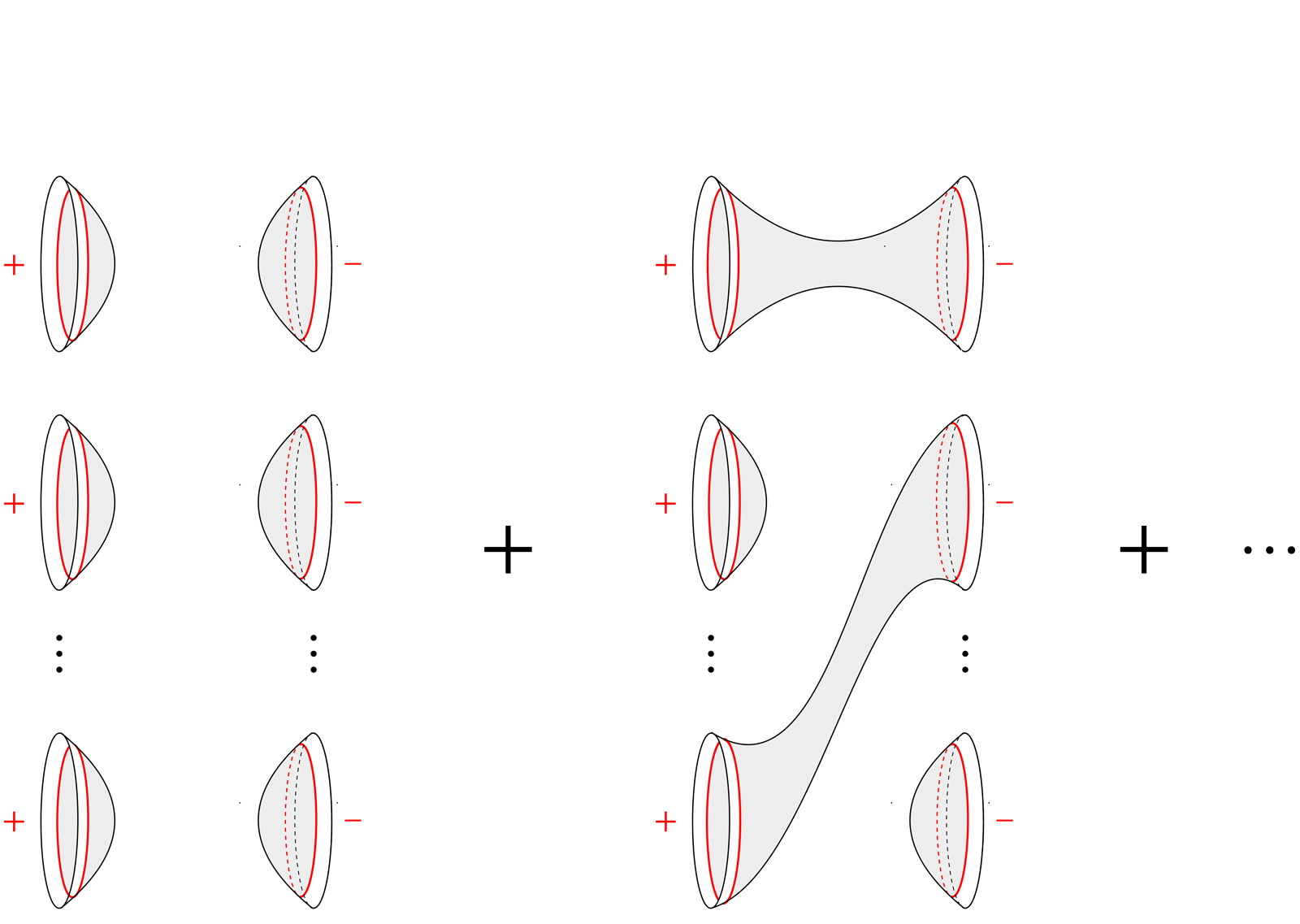
Figure 8: Computation of $\mathcal{P}(B^{m})$ in the replica trick for the free energy.

IV Discussion

One of the main motivation of this paper was to shed light on the holographic interpretation of Euclidean wormholes. We have shown how thermodynamic properties consistent with a wormhole can arise from averaging over complex couplings in the SYK model, and we have proposed a gravity interpretation as a Euclidean wormhole solution of JT gravity plus matter sharing similar properties.

We have studied the free energy of two copies of a system with complex conjugated Hamiltonians. This is also equal to the real part of the free energy of a single copy:

$$2\,\mathrm{Re}\,\langle F\rangle=-T\langle\log Z\bar{Z}\rangle~{}.$$ (42)

From the point of view of a single system, our wormhole can thus be seen as “real part wormhole” which connects the system to its complex conjugate in the gravitational computation of $\mathrm{Re}\,F$. The gravitational computation of the quenched free energy also involves replica wormholes which were computed in section III.3 and shown to be negligible in our setup.

The mechanism that makes the Euclidean wormhole possible is the introduction of imaginary sources for a marginal operator, which provides the negative energy necessary to sustain the wormhole. We emphasize that adding imaginary sources is perfectly consistent in Euclidean signature; it is akin to probing a system at imaginary chemical potential which, for example, has been useful to study QCD Roberge and Weiss (1986); de Forcrand and Philipsen (2002). We have identified a low temperature phase, where the wormhole dominates, and in which the marginal operator condenses. The non-zero expectation value of this operator is linked to the existence of the wormhole, since it vanishes in the black hole phase and becomes non-zero in the wormhole because of the source on the other boundary. This can be seen as a field theory diagnosis of the geometric connection in the bulk.

Our wormhole is different from the eternal traversable wormhole of Maldacena and Qi (2018), which makes sense as a Lorentzian geometry, and requires an explicit coupling between the boundaries. It’s also possible to introduce such an explicit coupling in our setup, in addition to the imaginary sources, and it would be interesting to study the resulting solutions.

In this paper, we have seen that imaginary sources can be used to support Euclidean wormhole solutions. As the comparison with SYK suggests, these sources might be related to some averaging procedure. It would be interesting to see whether other Euclidean wormholes can be constructed using this idea. Our solution extends to JT gravity with an additional gauge symmetry Iliesiu (2019); Kapec et al. (2020) or including the gravitational $\mathrm{U}(1)$ symmetry described in Godet and Marteau (2020). It should be possible to study multi-boundary solutions for which a dual SYK setup might exist. Euclidean wormholes have also found recent applications in AdS₃ holography Maxfield and Turiaci (2020); Maloney and Witten (2020); Afkhami-Jeddi et al. (2020); Cotler and Jensen (2020b); Belin and de Boer (2020) and it would be interesting to explore solutions in higher dimensions Cotler and Jensen (2020a).

Euclidean wormholes have played an important role in the study of eigenvalue statistics in pure JT gravity and in its field theory realization as a random matrix model Saad et al. (2018, 2019); Saad (2019); García-García and Zacarías (2019). The conclusion of these works is that JT gravity is quantum chaotic. Level statistics of quantum chaotic systems are described by random matrix theory. For the spectral form factor, a useful observable in spectral analysis, a signature of quantum chaos is the presence of a ramp for sufficiently long times that saturates at the Heisenberg time. In pure JT gravity, the spectral form factor is related to a double trumpet geometry which is not a solution of the equations of motion. An explicit evaluation of the path integral gives the contribution

$$\left\langle Z(\beta_{L})Z(\beta_{R})\right\rangle_{\mathrm{conn}}^{\mathrm{JT}}={1\over 2\pi}{\sqrt{\beta_{L}\beta_{R}}\over\beta_{L}+\beta_{R}}+\text{higher genus}~{},$$ (43)

which is actually the universal answer for a double-scaled random matrix integral. Replacing $\beta_{L}=\beta+it$ and $\beta_{R}=\beta-it$ leads to a contribution that grows linearly with $t$ for $t\gg\beta$ and accounts for the ramp in the spectral form factor. The same computation does not work for JT gravity plus matter as the integral over $b$ has a divergence at small $b$, seen here from the fact that $\mathcal{E}(b)\sim_{b\to 0}{\pi^{2}\over 6b^{2}}$. If we add imaginary sources, we can get around this issue by using our wormhole solution as a saddle point in this path integral. This suggests that Euclidean wormhole solutions, of the type constructed here, might be useful in studying the eigenvalue statistics of gravitational theories for which we cannot perform the full path integral. We leave this interesting question and the comparison with SYK level statistics to a future work.

Euclidean wormholes have also been important in understanding better the fine-grained entropy of evaporating black holes, where replica wormholes were crucial in obtaining an answer consistent with unitarity Penington et al. (2020); Almheiri et al. (2020a). It has also been argued that a gravitational replica trick is already needed for the computation of the free energy Engelhardt et al. (2020). We have implemented this replica trick in section III.3 to compute the free energy of our gravity setup and shown that the additional wormholes only give a negligible correction. It would be interesting to see whether wormhole solutions similar to the one described in this paper could be used as saddle points in the replica computation of the free energy in situations where they give large corrections, for example at very low temperatures.

On the field theory side, a non-Hermitian Hamiltonian is superficially related to a loss of probability conservation and a non-unitary evolution as most eigenvalues are complex and therefore have a finite lifetime. From the point of view of one of the two systems, this could be interpreted as the observation of particles coming in and coming out which is typical of an open quantum system. Although this is an appealing picture, it cannot really explain why a gap is observed. Ensemble average is a key ingredient for the formation of the gap at low temperatures so just a spectrum with imaginary eigenvalues is not enough to reproduce the observed phenomenology. As we mentioned earlier, another outstanding feature is that for sufficiently high temperature the non-Hermitian effects related to a complex spectrum becomes irrelevant. This suggests that the addition of an imaginary part in the SYK couplings, and the subsequent ensemble average, is just an effective way to describe quantum tunneling between two Hermitian SYK’s, and produces a gap between the ground state and the first excited state as in a double well potential. Typically, this is qualitatively modeled by an explicit coupling between the two SYK’s, as in the case the eternal traversable wormhole. However, we are interested in understanding better the issue of factorization, so we want to study configurations with an explicit coupling between the two systems.

Assuming that complex couplings and ensemble average are necessary ingredients to model tunneling without an explicit coupling, it would be interesting to determine the conditions on the field theory Hamiltonian that lead to this type of wormhole behavior. It seems that some form of randomness is required as wormhole-like features are only seen after an ensemble average. However, it is unclear whether infinite-range and strong interactions, as in the SYK model studied here, are also a necessary requirement.

Appendix A Quantum stress tensor in the double trumpet

In this section, we compute the quantum stress tensor of a massless scalar in the double trumpet geometry. We consider a free boson described by the action

$$S={1\over 2}\int d^{2}x\sqrt{g}\,(\partial\chi)^{2}~{},$$ (44)

and whose stress tensor is given by

$$T_{\mu\nu}=\partial_{\mu}\chi\partial_{\nu}\chi-{1\over 2}g_{\mu\nu}(\partial\chi)^{2}~{}.$$ (45)

To compute its expectation value, we use the point-splitting method so that

$$\langle T_{\mu\nu}(x)\rangle=\lim_{x^{\prime}\to x}\left(\partial_{\mu}\partial_{\nu}^{\prime}G(x,x^{\prime})-{1\over 2}g^{\mu\nu}\partial_{\mu}\partial_{\nu}^{\prime}G(x,x^{\prime})\right)~{},$$ (46)

where $G(x,x^{\prime})$ is the Green function. See Milton (2001); Freivogel et al. (2019) for examples of application of this method in related contexts. We will first perform the computation on a cylinder described by the coordinates

$$ds^{2}_{\mathrm{cyl}}=d\rho^{2}+d\theta^{2}~{},\qquad-{\pi\over 2}\leq\rho\leq{\pi\over 2}~{},\qquad\theta\sim\theta+b~{}.$$ (47)

We will then use a Weyl transformation to the double trumpet. The Green function can be defined as the solution of the equation

$$\Box_{x}G(x,x^{\prime})=-\delta(x-x^{\prime})~{}.$$ (48)

Using the following mode decomposition

$$G(\rho,\theta;\rho^{\prime},\theta^{\prime})=\sum_{\begin{subarray}{c}m,m^{\prime}\in\mathbb{Z}\end{subarray}}G(\rho,m;\rho^{\prime},m^{\prime})\,e^{2i\pi(m\theta+m^{\prime}\theta^{\prime})/b}~{},$$ (49)

the equation (48) becomes

$$\left(\partial_{\rho}^{2}-{4\pi^{2}m^{2}\over b^{2}}\right)G(\rho,m;\rho^{\prime},m^{\prime})=-{1\over b}\delta(\rho-\rho^{\prime})\delta_{m+m^{\prime}}~{},$$ (50)

with the boundary conditions

$$G(\rho,m;\rho^{\prime},m^{\prime})|_{\rho=\pm{\pi\over 2}}=G(\rho,m;\rho^{\prime},m^{\prime})|_{\rho^{\prime}=\pm{\pi\over 2}}=0~{}.$$ (51)

This can be solved using the discontinuity method, as explained in Milton (2001) for the standard Casimir effect between two plates. At the end, we find

$$G(\rho,\theta;\rho^{\prime},\theta^{\prime})=-\sum_{m\in\mathbb{Z}}{\mathrm{sinh}({2\pi m\over b}(\rho_{+}-\tfrac{\pi}{2}))\,\mathrm{sinh}({2\pi m\over b}(\rho_{-}+\tfrac{\pi}{2}))\over 2\pi m\,\mathrm{sinh}({2\pi^{2}m\over b})}e^{2i\pi m(\theta-\theta^{\prime})/b}~{},$$ (52)

which allows us to obtain

$$\langle T_{\rho\rho}\rangle=-\sum_{m\in\mathbb{Z}}{\pi m\over b^{2}\mathrm{tanh}\left({2\pi^{2}m\over b}\right)}~{},\qquad\langle T_{\theta\theta}\rangle=\sum_{m\in\mathbb{Z}}{\pi m\over b^{2}\mathrm{tanh}\left({2\pi^{2}m\over b}\right)}~{}.$$ (53)

The sum over $m$ can be regularized using the Poisson resummation formula, which allows us to write

$$S(x)\equiv\sum_{m\in\mathbb{Z}}{m\over\mathrm{tanh}(mx)}=-{\pi^{2}\over 2x^{2}}\sum_{n\in\mathbb{Z}}{1\over\mathrm{sinh}^{2}({\pi^{2}n\over x})}~{}.$$ (54)

We regulate the divergence at $n=0$ by imposing that in the limit $b\to+\infty$, we recover the known result for the strip. The final formula is

$$\langle T_{\theta\theta}\rangle=-\langle T_{\rho\rho}\rangle={c\over 24\pi}-{c\over\pi}\mathcal{E}(b)~{},$$ (55)

where have multiplied by an overall $c$ and defined

$$\mathcal{E}(b)\equiv\sum_{n\geq 1}{1\over 4\,\mathrm{sinh}^{2}({nb\over 2})}~{}.$$ (56)

We can now compute the stress tensor in the double trumpet using the formula

$$\langle T_{\mu\nu}\rangle=\langle T_{\mu\nu}\rangle_{\mathrm{cyl}}+\langle T_{\mu\nu}\rangle_{\mathrm{anomaly}}~{},$$ (57)

where the formula for the anomalous stress tensor is given in Brown and Cassidy (1977). This finally gives in the $(\tau,\rho)$ coordinates

$$\langle T_{\mu\nu}\rangle=-{1\over 24\pi}g_{\mu\nu}-{\mathcal{E}(b)\over\pi}\begin{pmatrix}1&0\\ 0&-1\end{pmatrix}~{}.$$ (58)

Some properties of the function $\mathcal{E}(b)$.

We give some properties of the function $\mathcal{E}(b)$ which appeared in the above computation. Firstly, we have $\mathcal{E}(b)>0$ and $\mathcal{E}(b)$ decreases with the following asymptotics:

$$\mathcal{E}(b)\underset{b\to 0}{\sim}{\pi^{2}\over 6b^{2}}~{},\qquad\mathcal{E}(b)\underset{b\to+\infty}{\sim}e^{-b}+O(e^{-2b})~{}.$$ (59)

After defining $q=e^{-b}$, we can write $\mathcal{E}(b)$ as

$$\mathcal{E}(b)=\sum_{n\geq 1}{q^{n}\over(1-q^{n})^{2}} = \sum_{n\geq 1}\sum_{m\geq 1}mq^{nm}=\sum_{m\geq 1}{mq^{m}\over 1-q^{m}}={1\over 24}(1-P(q))~{},$$ (60)

in terms of the function $P$ studied by Ramanujan Berndt (1985), which is related to the Dedekind eta function

$$P(q)=24q{d\over dq}\log\eta(q)~{},\qquad\eta(q)\equiv q^{1/24}\prod_{n\geq 1}(1-q^{n})~{}.$$ (61)

There is no simple analytic expression for $\mathcal{E}(b)$, but it can be expressed in a complicated way in terms of elliptic integrals Berndt (1998).

Appendix B Massive bulk fields

We have constructed a wormhole solution using a massless scalar field in the bulk, corresponding to an operator $\mathcal{O}$ with conformal dimension $\Delta=1$. In this Appendix, we consider massive fields and explain why $\Delta=1$ is the only value that gives a consistent solution.

The main point is that we need to satisfy the two boundary conditions of JT gravity:

$$\Phi={\bar{\phi}_{r}\over\epsilon},\qquad ds^{2}={du^{2}\over\epsilon^{2}}~{}.$$ (62)

Satisfying both in the double trumpet (8) requires that at leading order

$$\Phi\underset{\rho\to{\pi/2}}{\sim}{C\over{\pi\over 2}-\rho}~{},$$ (63)

where $C$ is some constant. Now, take $\chi$ to be a general massive scalar field satisfying the equation

$$(\Box-m^{2})\chi=0~{},\qquad m^{2}=\Delta(\Delta-1)~{}.$$ (64)

The pure imaginary sources give the condition

$$\chi\underset{\rho\to{\pi\over 2}}{\sim}ik\left({\pi\over 2}-\rho\right)^{1-\Delta},\qquad\chi\underset{\rho\to-{\pi\over 2}}{\sim}-ik\left({\pi\over 2}+\rho\right)^{1-\Delta}~{}.$$ (65)

This fixes the classical solution for $\chi$ which can be written explicitly in terms of hypergeometric functions.

We will focus on the low-temperature regime where the Casimir energy of $\chi$ can be ignored, which is the relevant regime for comparison with SYK. There, the equation of motion for the JT dilaton is

$$\nabla_{\mu}\nabla_{\nu}\Phi-g_{\mu\nu}\Box\Phi+g_{\mu\nu}\Phi+T_{\mu\nu}^{\chi}=0~{},\qquad T_{\mu\nu}^{\chi}=\partial_{\mu}\chi\partial_{\nu}\chi-{1\over 2}g_{\mu\nu}\left((\partial\chi)^{2}+m^{2}\chi^{2}\right)~{}.$$ (66)

Taking the trace of this equation gives

$$(\Box-2)\Phi=-\Delta(\Delta-1)\chi^{2}~{}.$$ (67)

From (63), we can verify

$$\lim_{\rho\to{\pi\over 2}}(\Box-2)\Phi=\text{finite constant}~{},$$ (68)

where the constant depends on subleading terms in $\Phi$. This is only compatible with $\Delta=1$ because otherwise $\chi^{2}\sim\left({\pi\over 2}-\rho\right)^{-2(\Delta-1)}$ diverges for $\rho\to{\pi\over 2}$. This shows that a wormhole solution can be obtained in this way only for $\Delta=1$.

References

- Lavrelashvili et al. (1987) George V. Lavrelashvili, V.A. Rubakov, and P.G. Tinyakov, “Disruption of Quantum Coherence upon a Change in Spatial Topology in Quantum Gravity,” JETP Lett. 46, 167–169 (1987).
- Hawking (1987) S.W. Hawking, “Quantum Coherence Down the Wormhole,” Phys. Lett. B 195, 337 (1987).
- Giddings and Strominger (1988a) Steven B. Giddings and Andrew Strominger, “Axion Induced Topology Change in Quantum Gravity and String Theory,” Nucl. Phys. B 306, 890–907 (1988a).
- Giddings and Strominger (1988b) Steven B. Giddings and Andrew Strominger, “Loss of incoherence and determination of coupling constants in quantum gravity,” Nuclear Physics B 307, 854 – 866 (1988b).
- Giddings and Strominger (1989) Steven B Giddings and Andrew Strominger, “Baby universe, third quantization and the cosmological constant,” Nuclear Physics B 321, 481 – 508 (1989).
- Coleman (1988) Sidney R. Coleman, “Why There Is Nothing Rather Than Something: A Theory of the Cosmological Constant,” Nucl. Phys. B 310, 643–668 (1988).
- Maldacena and Maoz (2004) Juan Maldacena and Liat Maoz, “Wormholes in AdS,” Journal of High Energy Physics 2004, 053–053 (2004).
- Arkani-Hamed et al. (2007) Nima Arkani-Hamed, Luboš Motl, Alberto Nicolis, and Cumrun Vafa, “The string landscape, black holes and gravity as the weakest force,” Journal of High Energy Physics 2007, 060–060 (2007).
- Hertog et al. (2019) Thomas Hertog, Brecht Truijen, and Thomas Van Riet, “Euclidean axion wormholes have multiple negative modes,” Phys. Rev. Lett. 123, 081302 (2019), arXiv:1811.12690 [hep-th] .
- Hebecker et al. (2018) Arthur Hebecker, Thomas Mikhail, and Pablo Soler, “Euclidean wormholes, baby universes, and their impact on particle physics and cosmology,” Front. Astron. Space Sci. 5, 35 (2018), arXiv:1807.00824 [hep-th] .
- Jackiw (1985) Roman Jackiw, “Lower dimensional gravity,” Nuclear Physics B 252, 343 – 356 (1985).
- Teitelboim (1983) Claudio Teitelboim, “Gravitation and hamiltonian structure in two spacetime dimensions,” Physics Letters B 126, 41 – 45 (1983).
- Jensen (2016) Kristan Jensen, “Chaos in holography,” Phys. Rev. Lett. 117, 111601 (2016).
- Maldacena et al. (2016) Juan Maldacena, Douglas Stanford, and Zhenbin Yang, “Conformal symmetry and its breaking in two-dimensional nearly anti-de sitter space,” Progress of Theoretical and Experimental Physics 2016, 12C104 (2016).
- Engelsöy et al. (2016) Julius Engelsöy, Thomas G. Mertens, and Herman Verlinde, “An investigation of ads2 backreaction and holography,” Journal of High Energy Physics 07, 1–30 (2016).
- Saad et al. (2018) Phil Saad, Stephen H. Shenker, and Douglas Stanford, “A semiclassical ramp in SYK and in gravity,” (2018), arXiv:1806.06840 [hep-th] .
- Saad et al. (2019) Phil Saad, Stephen H. Shenker, and Douglas Stanford, “JT gravity as a matrix integral,” (2019), arXiv:1903.11115 [hep-th] .
- Saad (2019) Phil Saad, “Late Time Correlation Functions, Baby Universes, and ETH in JT Gravity,” (2019), arXiv:1910.10311 [hep-th] .
- Penington (2020) Geoffrey Penington, “Entanglement Wedge Reconstruction and the Information Paradox,” JHEP 09, 002 (2020), arXiv:1905.08255 [hep-th] .
- Almheiri et al. (2019) Ahmed Almheiri, Netta Engelhardt, Donald Marolf, and Henry Maxfield, “The entropy of bulk quantum fields and the entanglement wedge of an evaporating black hole,” JHEP 12, 063 (2019), arXiv:1905.08762 [hep-th] .
- Penington et al. (2020) Geoff Penington, Stephen H. Shenker, Douglas Stanford, and Zhenbin Yang, “Replica wormholes and the black hole interior,” (2020), arXiv:1911.11977 [hep-th] .
- Almheiri et al. (2020a) Ahmed Almheiri, Thomas Hartman, Juan Maldacena, Edgar Shaghoulian, and Amirhossein Tajdini, “Replica wormholes and the entropy of hawking radiation,” Journal of High Energy Physics 2020 (2020a), 10.1007/jhep05(2020)013.
- Almheiri et al. (2020b) Ahmed Almheiri, Thomas Hartman, Juan Maldacena, Edgar Shaghoulian, and Amirhossein Tajdini, “The entropy of hawking radiation,” (2020b), arXiv:2006.06872 [hep-th] .
- Blommaert et al. (2019) Andreas Blommaert, Thomas G. Mertens, and Henri Verschelde, “Eigenbranes in Jackiw-Teitelboim gravity,” (2019), arXiv:1911.11603 [hep-th] .
- Betzios et al. (2019) P. Betzios, E. Kiritsis, and O. Papadoulaki, “Euclidean Wormholes and Holography,” JHEP 06, 042 (2019), arXiv:1903.05658 [hep-th] .
- Marolf and Maxfield (2020) Donald Marolf and Henry Maxfield, “Transcending the ensemble: baby universes, spacetime wormholes, and the order and disorder of black hole information,” Journal of High Energy Physics 2020 (2020), 10.1007/jhep08(2020)044.
- Pollack et al. (2020) Jason Pollack, Moshe Rozali, James Sully, and David Wakeham, “Eigenstate Thermalization and Disorder Averaging in Gravity,” Phys. Rev. Lett. 125, 021601 (2020), arXiv:2002.02971 [hep-th] .
- Raamsdonk (2020) Mark Van Raamsdonk, “Comments on wormholes, ensembles, and cosmology,” (2020), arXiv:2008.02259 [hep-th] .
- Betzios and Papadoulaki (2020) Panagiotis Betzios and Olga Papadoulaki, “Liouville theory and Matrix models: A Wheeler DeWitt perspective,” JHEP 09, 125 (2020), arXiv:2004.00002 [hep-th] .
- Giddings and Turiaci (2020) Steven B. Giddings and Gustavo J. Turiaci, “Wormhole calculus, replicas, and entropies,” (2020), arXiv:2004.02900 [hep-th] .
- Blommaert (2020) Andreas Blommaert, “Dissecting the ensemble in JT gravity,” (2020), arXiv:2006.13971 [hep-th] .
- Anous et al. (2020) Tarek Anous, Jorrit Kruthoff, and Raghu Mahajan, “Density matrices in quantum gravity,” SciPost Phys. 9, 045 (2020), arXiv:2006.17000 [hep-th] .
- Chen et al. (2020) Yiming Chen, Victor Gorbenko, and Juan Maldacena, “Bra-ket wormholes in gravitationally prepared states,” (2020), arXiv:2007.16091 [hep-th] .
- Eberhardt (2020) Lorenz Eberhardt, “Partition functions of the tensionless string,” (2020), arXiv:2008.07533 [hep-th] .
- Stanford (2020) Douglas Stanford, “More quantum noise from wormholes,” (2020), arXiv:2008.08570 [hep-th] .
- McNamara and Vafa (2020) Jacob McNamara and Cumrun Vafa, “Baby Universes, Holography, and the Swampland,” (2020), arXiv:2004.06738 [hep-th] .
- Alishahiha et al. (2020) Mohsen Alishahiha, Amin Faraji Astaneh, Ghadir Jafari, Ali Naseh, and Behrad Taghavi, “On free energy for deformed jt gravity,” (2020), arXiv:2010.02016 [hep-th] .
- Cotler and Jensen (2020a) Jordan Cotler and Kristan Jensen, “Gravitational Constrained Instantons,” (2020a), arXiv:2010.02241 [hep-th] .
- Maldacena (2003) Juan Maldacena, “Eternal black holes in anti-de sitter,” Journal of High Energy Physics 2003, 021–021 (2003).
- Maldacena and Susskind (2013) Juan Maldacena and Leonard Susskind, “Cool horizons for entangled black holes,” Fortsch. Phys. 61, 781–811 (2013), arXiv:1306.0533 [hep-th] .
- Gao et al. (2017) Ping Gao, Daniel Louis Jafferis, and Aron Wall, “Traversable Wormholes via a Double Trace Deformation,” JHEP 12, 151 (2017), arXiv:1608.05687 [hep-th] .
- Maldacena et al. (2017) Juan Maldacena, Douglas Stanford, and Zhenbin Yang, “Diving into traversable wormholes,” Fortsch. Phys. 65, 1700034 (2017), arXiv:1704.05333 [hep-th] .
- Maldacena and Qi (2018) Juan Maldacena and Xiao-Liang Qi, “Eternal traversable wormhole,” (2018), arXiv:1804.00491 [hep-th] .
- Bak et al. (2018) Dongsu Bak, Chanju Kim, and Sang-Heon Yi, “Bulk view of teleportation and traversable wormholes,” JHEP 08, 140 (2018), arXiv:1805.12349 [hep-th] .
- Kim et al. (2019) Jaewon Kim, Igor R. Klebanov, Grigory Tarnopolsky, and Wenli Zhao, “Symmetry Breaking in Coupled SYK or Tensor Models,” (2019), arXiv:1902.02287 [hep-th] .
- French and Wong (1970) J.B. French and S.S.M. Wong, “Validity of random matrix theories for many-particle systems,” Physics Letters B 33, 449 – 452 (1970).
- Bohigas and Flores (1971) O. Bohigas and J. Flores, “Two-body random hamiltonian and level density,” Physics Letters B 34, 261 – 263 (1971).
- Sachdev and Ye (1993) Subir Sachdev and Jinwu Ye, “Gapless spin-fluid ground state in a random quantum heisenberg magnet,” Phys. Rev. Lett. 70, 3339–3342 (1993).
- (49) Alexander Kitaev, “A simple model of quantum holography,” KITP strings seminar and Entanglement 2015 program, 12 February, 7 April and 27 May 2015, http://online.kitp.ucsb.edu/online/entangled15/.
- Maldacena and Stanford (2016) Juan Maldacena and Douglas Stanford, “Remarks on the sachdev-ye-kitaev model,” Phys. Rev. D 94, 106002 (2016).
- Jevicki et al. (2016) Antal Jevicki, Kenta Suzuki, and Junggi Yoon, “Bi-local holography in the syk model,” Journal of High Energy Physics 07, 1–25 (2016).
- García-García and Verbaarschot (2016) Antonio M. García-García and Jacobus J. M. Verbaarschot, “Spectral and thermodynamic properties of the sachdev-ye-kitaev model,” Phys. Rev. D 94, 126010 (2016).
- García-García and Verbaarschot (2017) Antonio M. García-García and Jacobus J. M. Verbaarschot, “Analytical spectral density of the sachdev-ye-kitaev model at finite ,” Phys. Rev. D 96, 066012 (2017).
- Bagrets et al. (2016) Dmitry Bagrets, Alexander Altland, and Alex Kamenev, “Sachdev–ye–kitaev model as liouville quantum mechanics,” Nuclear Physics B 911, 191–205 (2016).
- Bagrets et al. (2017) Dmitry Bagrets, Alexander Altland, and Alex Kamenev, “Power-law out of time order correlation functions in the syk model,” Nuclear Physics B 921, 727 – 752 (2017).
- García-García et al. (2019) Antonio M. García-García, Tomoki Nosaka, Dario Rosa, and Jacobus J. M. Verbaarschot, “Quantum chaos transition in a two-site sachdev-ye-kitaev model dual to an eternal traversable wormhole,” Phys. Rev. D 100, 026002 (2019).
- Almheiri and Polchinski (2015) Ahmed Almheiri and Joseph Polchinski, “Models of ads2 backreaction and holography,” Journal of High Energy Physics 11, 1–19 (2015).
- Almheiri and Kang (2016) Ahmed Almheiri and Byungwoo Kang, “Conformal Symmetry Breaking and Thermodynamics of Near-Extremal Black Holes,” JHEP 10, 052 (2016), arXiv:1606.04108 [hep-th] .
- Nayak et al. (2018) Pranjal Nayak, Ashish Shukla, Ronak M. Soni, Sandip P. Trivedi, and V. Vishal, “On the Dynamics of Near-Extremal Black Holes,” JHEP 09, 048 (2018), arXiv:1802.09547 [hep-th] .
- Castro and Godet (2020) Alejandra Castro and Victor Godet, “Breaking away from the near horizon of extreme Kerr,” SciPost Phys. 8, 089 (2020), arXiv:1906.09083 [hep-th] .
- Engelhardt and Horowitz (2016) Netta Engelhardt and Gary T. Horowitz, “Holographic Consequences of a No Transmission Principle,” Phys. Rev. D 93, 026005 (2016), arXiv:1509.07509 [hep-th] .
- Freivogel et al. (2019) Ben Freivogel, Victor Godet, Edward Morvan, Juan F. Pedraza, and Antonio Rotundo, “Lessons on Eternal Traversable Wormholes in AdS,” JHEP 07, 122 (2019), arXiv:1903.05732 [hep-th] .
- Roberge and Weiss (1986) Andre Roberge and Nathan Weiss, “Gauge Theories With Imaginary Chemical Potential and the Phases of {QCD},” Nucl. Phys. B 275, 734–745 (1986).
- de Forcrand and Philipsen (2002) Philippe de Forcrand and Owe Philipsen, “The QCD phase diagram for small densities from imaginary chemical potential,” Nucl. Phys. B 642, 290–306 (2002), arXiv:hep-lat/0205016 .
- Engelhardt et al. (2020) Netta Engelhardt, Sebastian Fischetti, and Alexander Maloney, “Free energy from replica wormholes,” (2020), arXiv:2007.07444 [hep-th] .
- Iliesiu (2019) Luca V. Iliesiu, “On 2D gauge theories in Jackiw-Teitelboim gravity,” (2019), arXiv:1909.05253 [hep-th] .
- Kapec et al. (2020) Daniel Kapec, Raghu Mahajan, and Douglas Stanford, “Matrix ensembles with global symmetries and ’t Hooft anomalies from 2d gauge theory,” JHEP 04, 186 (2020), arXiv:1912.12285 [hep-th] .
- Godet and Marteau (2020) Victor Godet and Charles Marteau, “New boundary conditions for AdS2,” (2020), arXiv:2005.08999 [hep-th] .
- Maxfield and Turiaci (2020) Henry Maxfield and Gustavo J. Turiaci, “The path integral of 3D gravity near extremality; or, JT gravity with defects as a matrix integral,” (2020), arXiv:2006.11317 [hep-th] .
- Maloney and Witten (2020) Alexander Maloney and Edward Witten, “Averaging Over Narain Moduli Space,” (2020), arXiv:2006.04855 [hep-th] .
- Afkhami-Jeddi et al. (2020) Nima Afkhami-Jeddi, Henry Cohn, Thomas Hartman, and Amirhossein Tajdini, “Free partition functions and an averaged holographic duality,” (2020), arXiv:2006.04839 [hep-th] .
- Cotler and Jensen (2020b) Jordan Cotler and Kristan Jensen, “AdS3 gravity and random CFT,” (2020b), arXiv:2006.08648 [hep-th] .
- Belin and de Boer (2020) Alexandre Belin and Jan de Boer, “Random Statistics of OPE Coefficients and Euclidean Wormholes,” (2020), arXiv:2006.05499 [hep-th] .
- García-García and Zacarías (2019) Antonio M. García-García and Salomón Zacarías, “Quantum jackiw-teitelboim gravity, selberg trace formula, and random matrix theory,” (2019), arXiv:1911.10493 [hep-th] .
- Milton (2001) K.A. Milton, The Casimir effect: Physical manifestations of zero-point energy (2001).
- Brown and Cassidy (1977) Lowell S. Brown and James P. Cassidy, “Stress Tensors and their Trace Anomalies in Conformally Flat Space-Times,” Phys. Rev. D 16, 1712 (1977).
- Berndt (1985) B.C. Berndt, Ramanujan’s Notebooks, dl. 1 (Springer New York, 1985).
- Berndt (1998) Bruce C. Berndt, “Ramanujan’s theories of elliptic functions to alternative bases,” in Ramanujan’s Notebooks: Part V (Springer New York, New York, NY, 1998) pp. 89–181.