The Primal-Dual method for Learning Augmented Algorithms

Abstract

The extension of classical online algorithms when provided with predictions is a new and active research area. In this paper, we extend the primal-dual method for online algorithms in order to incorporate predictions that advise the online algorithm about the next action to take. We use this framework to obtain novel algorithms for a variety of online covering problems. We compare our algorithms to the cost of the true and predicted offline optimal solutions and show that these algorithms outperform any online algorithm when the prediction is accurate while maintaining good guarantees when the prediction is misleading.

1 Introduction

In the classical field of online algorithms the input is presented in an online fashion and the algorithm is required to make irrevocable decisions without knowing the future. The performance is often measured in terms of worst-case guarantees with respect to an optimal offline solution. In this paper, we will consider minimization problems and formally, we will say that an online algorithm $\mathcal{ALG}$ is $c$-competitive if on any input $\mathcal{I}$, the cost $c_{\mathcal{ALG}}(\mathcal{I})$ of the solution output by algorithm $\mathcal{ALG}$ on input $\mathcal{I}$ satisfies $c_{\mathcal{ALG}}(\operatorname{\mathcal{I}})\leqslant c\cdot\operatorname{OPT}(\mathcal{I})$, where $\operatorname{OPT}(\mathcal{I})$ denotes the cost of the offline optimum. Due to the uncertainty about the future, online algorithms tend to be overly cautious which sometimes causes their performance in real-world situations to be far from what a machine learning (ML) algorithm would have achieved. Indeed in many practical applications future events follow patterns which are easily predictable using ML methods. In [19] Lykouris and Vassilvitskii formalized a general framework for incorporating (ML) predictions into online algorithms and designed an extension of the marking algorithm to solve the online caching problem when provided with predictions. This work was quickly followed by many other papers studying different learning augmented online problems such as scheduling ([17]), caching ([2, 26]), ski rental ([16, 10, 28, 25]), clustering ([7]) and other problems ([23, 12]). The main challenge is to incorporate the prediction without knowing how the prediction was computed and in particular without making any assumption on the quality of the prediction. This setting is natural as in real-world situations, predictions are provided by ML algorithms that rarely come with worst-case guarantees on their accuracy. Thus, the difficulty in designing a learning augmented algorithm is to find a good balance: on the one hand, following blindly the prediction might lead to a very bad solution if the prediction is misleading. On the other hand if the algorithm does not trust the prediction at all, it will simply never benefit from an excellent prediction. The aforementioned results solve this issue by designing smart algorithms which exploit the problem structure to achieve a good trade-off between these two cases. In this paper we take a different perspective. Instead of focusing on a specific problem trying to integrate predictions, we show how to extend a very powerful algorithmic method, the Primal-Dual method, into the design of online learning augmented algorithms. We underline that despite the generality of our extension technique, it produces online learning augmented algorithms in a fairly simple and straightforward manner.

The Primal-Dual method. The Primal-Dual (PD) method is a very powerful algorithmic technique to design online algorithms. It was first introduced by Alon et al. [1] to design an online algorithm for the classical online set cover problem and later extended to many other problems such as weighted caching ([3]), revenue maximization in ad-auctions, TCP acknowledgement and ski rental [5]. We mention the survey of Buchbinder and Naor [4] for more references about this technique. In a few words, the technique consists in formulating the online problem as a linear program $P$ complemented by its dual $D$. Subsequently, the algorithm builds online a feasible fractional solution to both the primal $P$ and dual $D$. Every time an update of the primal and dual variables is made, the cost of the primal increases by some amount $\Delta P$ while the cost of the dual increases by some amount $\Delta D$. The competitive ratio of the fractional solution is then obtained by upper bounding the ratio $\frac{\Delta P}{\Delta D}$ and using weak duality. The integral solution is then obtained by an online rounding scheme of the fractional solution.

Preliminary notions for Learning Augmented (LA) algorithms. LA algorithms receive as input a prediction $\operatorname{\mathcal{A}}$, an instance $\mathcal{I}$ which is revealed online, a robustness parameter $\lambda$, and output a solution of cost $c_{\mathcal{ALG}}(\operatorname{\mathcal{A}},\operatorname{\mathcal{I}},\lambda)$. Intuitively, $\lambda$ indicates our confidence in the prediction with smaller values reflecting high confidence. We denote by $S\left(\mathcal{A,\mathcal{I}}\right)$ the cost of the output solution on input $\mathcal{I}$ if the algorithm follows blindly the prediction $\mathcal{A}$. We avoid defining explicitly prediction $\operatorname{\mathcal{A}}$ to easily fit different prediction cases. For instance if the prediction $\mathcal{A}$ is a predicted solution (without necessarily revealing the predicted instance) then following blindly the solution would simply mean to output the predicted solution $\mathcal{A}$. For each result presented in this paper, it will be clear what is the prediction $\mathcal{A}$ and the cost $S(\operatorname{\mathcal{A}},\operatorname{\mathcal{I}})$. Given this, we restate some useful definitions introduced in [19, 25] in our context. For any $0<\lambda\leqslant 1$, we will say that an LA algorithm is $C(\lambda)$-consistent and $R(\lambda)$-robust if the cost of the output solution satisfies:

$$c_{\mathcal{ALG}}(\operatorname{\mathcal{A}},\mathcal{I},\lambda)\leqslant\min\left\{C(\lambda)\cdot S(\operatorname{\mathcal{A}},\mathcal{I}),R(\lambda)\cdot\operatorname{OPT}(\operatorname{\mathcal{I}})\right\}$$ (1)

If $\operatorname{\mathcal{A}}$ is accurate ($S(\operatorname{\mathcal{A}},\operatorname{\mathcal{I}})\approx\operatorname{OPT}(\operatorname{\mathcal{I}})$) and at the same time we trust the prediction, we would like our performance to be close to the optimal offline. Thus, ideally $C(\lambda)$ should approach $1$ as $\lambda$ approaches $0$. On the same spirit, a value of $\lambda$ close to $1$ denotes no trust to the prediction, and in that case, our algorithm should not be much worse than the best pure online algorithm. Therefore, $R(1)$ should be close to the competitive ratio of the best pure online algorithm. We also mention that in some other papers such as [25], a smoothness criterion on the consistency bound is required. In these papers the setting is slightly different. Indeed, prediction $\operatorname{\mathcal{A}}$ is a predicted instance $\operatorname{\mathcal{I}}^{\textit{pred}}$ and the error is defined to describe how far $\operatorname{\mathcal{I}}^{\textit{pred}}$ is from the real instance $\operatorname{\mathcal{I}}$. With this in mind, an algorithm is said to be smooth if the performance degrades smoothly as the error increases. We emphasize that, in the applications considered in this paper, this smoothness property is implicitly included in the value of $S(\operatorname{\mathcal{A}},\mathcal{I})$ which degrades smoothly with the quality of the prediction.

Our contributions.

We show how to extend the Primal-Dual method (when predictions are provided) for solving problems that can be formulated as covering problems. The algorithms designed using this technique receive as input a robustness parameter $\lambda$ and incorporate a prediction. If the prediction is accurate our algorithms can be arbitrarily close to the optimal offline (beating known lower bounds of the classical online algorithms) while being robust to failures of the predictor. We first apply our Primal-Dual Learning Augmented (PDLA) technique to the online version of the weighted set cover problem, which constitutes the most canonical example of a covering Linear Program (LP). For that problem we show how we can easily modify the Primal-Dual algorithm to incorporate predictions. Even though in this case, prediction may not seem very natural, this result reveals that we can use PDLA to design learning augmented algorithms for the large class of problems that can be formulated as a covering LP. We then continue by addressing problems in which the prediction model is much more natural. Using the PDLA technique, we first design an algorithm which recovers the results of Purohit et al. [25] for the ski rental problem, and we also prove that the consistency-robustness trade-off of that algorithm is optimal. We additionally design a learning augmented algorithm for a generalization of the ski rental, namely the Bahncard problem. Finally, we turn our attention to a problem which arises in network congestion control, the TCP acknowledgement problem. We design an LA algorithm for that problem and conduct experiments which confirm our claims. We note that the analysis of the algorithms designed using PDLA is (arguably) simple and boils down to (1) proving robustness with (essentially) the same proof as in the original Primal-Dual technique and (2) proving consistency using a simple charging argument that, without making use of the dual, relates the cost incurred by our algorithms to the prediction. In addition to that, using PDLA, the design of online LA algorithms is almost automatic. We emphasize that the preexisting online rounding schemes to obtain an integral solution from a fractional solution still apply to our learning augmented algorithms. Hence in all the paper we focus only on building a fractional solution and provide appropriate references for the rounding scheme.

2 General PDLA method

In this section we apply PDLA to solve the online weighted set cover problem when provided with predictions. Set cover is arguably the most canonical example of a covering problem and the framework that we develop readily applies to other covering problems. In particular, we use the framework to give tight or nearly-tight LA algorithms for ski rental, Bahncard, and dynamic TCP acknowledgement, which are all problems that can be formulated as covering LPs.

Figure 1: Primal Dual formulation of weighted set cover

The weighted set cover problem.

In this problem, we are given a universe $\mathcal{U}=\{e_{1},e_{2},\dots,e_{n}\}$ of $n$ elements and a family $\mathcal{F}$ of $m$ sets over this universe, each set $S\in\mathcal{F}$ has a weight $w_{S}$ and each element $e$ is covered by any set in $\operatorname{\mathcal{F}}(e)=\{S\in\operatorname{\mathcal{F}}\mid e\in S\}$. Let ${d=\max_{e\in\mathcal{U}}|\mathcal{F}(e)|}$ denote the maximum number of sets that cover one element. Our goal is to select sets so as to cover all elements while minimizing the total weight. In its online version, elements are given one by one and it is unknown to the algorithm which elements will arrive and in which order. When a new element arrives, it is required to cover it by adding a new set if necessary. Removing a set from the current solution to decrease its cost is not allowed. Alon et al. in [1] first studied the online version designing an almost optimal ${O(\log n\log d)}$-competitive algorithm. We note that the $O(\log n)$ factor comes from the integrality gap of the linear program formulation of the problem (Figure 1) while the $O(\log d)$ is due to the online nature of the problem. Since Alon et al. [1] designed an online rounding scheme at a multiplicative cost of $O(\log n)$, we will focus on building an increasing fractional solution to the set cover problem (i.e. $x_{S}$ can only increase over time for all $S$).

PDLA for weighted set cover.

Algorithm 2 takes as input a predicted covering $\operatorname{\mathcal{A}}\subset\operatorname{\mathcal{F}}$ and a robustness parameter $\lambda\in\left[0,1\right]$. While an instance $\operatorname{\mathcal{I}}$ is revealed in an online fashion, an increasing fractional solution ${\{x_{S}\}_{S\in\operatorname{\mathcal{F}}}\in{[0,1]}^{\operatorname{\mathcal{F}}}}$ is built. Note that $\operatorname{\mathcal{F}}(e)\cap\operatorname{\mathcal{A}}$ are the sets which cover $e$ in the prediction. To simplify the description, we assume that ${|\operatorname{\mathcal{F}}(e)\cap\operatorname{\mathcal{A}}|\geqslant 1},\forall e$, i.e. the prediction forms a feasible solution. The algorithm without this assumption can be found in appendix A.

Algorithm Intuition.

We first turn our attention to the original online algorithm of Alon et. al. [1] described in Algorithm 1. To get an intuition assume that $w_{S}=1,\forall S$ and consider the very first arrival of an element $e$. After the first execution of the while loop, $e$ is covered and ${x_{S}=\frac{1}{|\operatorname{\mathcal{F}}(e)|},\forall S\in\operatorname{\mathcal{F}}(e)}$. In other words, the online algorithm creates a uniform distribution over the sets in $\operatorname{\mathcal{F}}(e)$, reflecting in such a way his unawareness about the future. On the contrary Algorithm 2 uses the prediction to adjust the increase rate of primal variables, augmenting more aggressively primal variables of sets which are predicted to be in the optimal offline solution. Indeed, after the first execution of the while loop, sets which belong to $\operatorname{\mathcal{A}}$ get a value of ${\frac{\lambda}{|\operatorname{\mathcal{F}}(e)|}+\frac{1-\lambda}{|{\operatorname{\mathcal{F}}}(e)\cap\operatorname{\mathcal{A}}|}}$ while sets which are not chosen by the prediction get $\frac{\lambda}{|\operatorname{\mathcal{F}}(e)|}$.

black$\Rightarrow$

Algorithm 1 Primal Dual Method for Online Weighted Set Cover [1].

  Initialize: $x_{S}\leftarrow 0$, $y_{e}\leftarrow 0$ $\forall S,e$

  for all element $e$ that just arrived do

     while $\sum_{S\in\operatorname{\mathcal{F}}(e)}x_{S}<1$ do

        /* Primal Update

        for all $S\in\operatorname{\mathcal{F}}(e)$ do

           $x_{S}\leftarrow x_{S}\left(1+\frac{1}{w_{S}}\right)+\frac{1}{w_{S}|\operatorname{\mathcal{F}}(e)|}$

        end for

        /* Dual Update

        $y_{e}\leftarrow y_{e}+1$

     end while

  end for

Algorithm 2 PDLA for Online Weighted Set Cover.

  Input: $\lambda$, $\operatorname{\mathcal{A}}$

  Initialize: $x_{S}\leftarrow 0$, $y_{e}\leftarrow 0$ $\forall S,e$

  for all element $e$ that just arrived do

    while $\sum_{S\in\operatorname{\mathcal{F}}(e)}x_{S}<1$ do

       /* Primal Update

       for all $S\in\operatorname{\mathcal{F}}(e)$ and $S\in\operatorname{\mathcal{A}}$ do

          ${x_{S}\leftarrow x_{S}\!\left(\!1+\!\!\frac{1}{w_{S}}\right)\!+\!\frac{\lambda}{w_{S}|\operatorname{\mathcal{F}}(e)|}\!\!+\!\!\frac{1-\lambda}{w_{S}|\operatorname{\mathcal{F}}(e)\cap\operatorname{\mathcal{A}}|}}$

       end for

       for all $S\in\operatorname{\mathcal{F}}(e)$ and $S\not\in\operatorname{\mathcal{A}}$ do

          $x_{S}\leftarrow x_{S}\left(1+\frac{1}{w_{S}}\right)+\frac{\lambda}{w_{S}|\operatorname{\mathcal{F}}(e)|}$

       end for

       /* Dual Update

       $y_{e}\leftarrow y_{e}+1$

    end while

  end for

We continue by exposing our main conceptual contribution. To that end let $S(\operatorname{\mathcal{A}},\operatorname{\mathcal{I}})$ denote the cost of the covering solution described by prediction $\operatorname{\mathcal{A}}$ on instance $\operatorname{\mathcal{I}}$.

Theorem 1.

Assuming $\operatorname{\mathcal{A}}$ is a feasible solution, the cost of the fractional solution output by Algorithm 2 satisfies

$$c_{\tiny\mathcal{PDLA}}(\mathcal{A},\mathcal{I},\lambda)\leqslant\min\left\{O\left(\frac{1}{1-\lambda}\right)\cdot S(\operatorname{\mathcal{A}},\operatorname{\mathcal{I}}),O\left(\log\left(\frac{d}{\lambda}\right)\right)\cdot\operatorname{OPT}(\operatorname{\mathcal{I}})\right\}$$

Proof sketch..

The proof is split in two parts. The first part is to bound the cost of the algorithm by the term ${O\left(\frac{1}{1-\lambda}\right)\cdot S(\operatorname{\mathcal{A}},\operatorname{\mathcal{I}})}$. As mentioned in the introduction we use a charging argument to do so. After each execution of the while loop we can decompose the primal increase into two parts. $\Delta P_{c}$ which denotes the increase due to sets in $\operatorname{\mathcal{F}}(e)\cap\operatorname{\mathcal{A}}$ and $\Delta P_{u}$ which denotes the increase due to sets in $\operatorname{\mathcal{F}}(e)\setminus\operatorname{\mathcal{A}}$, thus for the overall primal increase $\Delta P$ we have $\Delta P=\Delta P_{c}+\Delta P_{u}$. We continue by upper bounding $\Delta P_{u}$ as a function of $\lambda$ and $\Delta P_{c}$, that is $\Delta P_{u}\leqslant O(\frac{1+\lambda}{1-\lambda})\Delta P_{c}$, and deducing that ${\Delta P\leqslant O(\frac{1}{1-\lambda})\Delta P_{c}}$. Now the consistency proof terminates by noting that since $\Delta P_{c}$ is generated by sets in the prediction, we can charge this increase to $S(\operatorname{\mathcal{A}},\operatorname{\mathcal{I}})$. The robustness bound, which is independent of the prediction, is retrieved by mimicking the proof of the original online algorithm of Alon et al. [1]. See appendix A for more details. ∎

3 The Ski rental problem

Figure 2: Primal dual formulation of the ski rental problem.

As another application of PDLA we design a learning augmented algorithm for one of the simplest and well studied online problems, the ski rental problem. In this problem, every new day, one has to decide whether to rent skis for this day, which costs $1$ dollar or to buy skis for the rest of the vacation at a cost of $B$ dollars. In its offline version the total number of vacation days, $N$, is known in advance and the problem becomes trivial. From the primal-dual formulation of the problem (Figure 2) it is clear that if $B<N$, the optimal strategy is to buy the skis at day one while if $B\geqslant N$ the optimal strategy is to always rent. In the online setting the difficulty relies in the fact that we do not know $N$ in advance. A deterministic $2$-competitive online algorithm has been known for a long time [13] and a randomized $\frac{e}{e-1}\approx 1.58$-competitive algorithm was also designed later [14]. Both competitive ratios are known to be optimal for deterministic and randomized algorithms respectively. This problem was already studied in various learning augmented settings [25, 10, 16, 28]. Our approach recovers, using the primal-dual method, the results of [25]. As in [25] our prediction $\operatorname{\mathcal{A}}$ will be the total number of vacation days $N^{\textit{pred}}$.

PDLA for ski rental.

To simplify the description, we denote an instance of the problem as ${\operatorname{\mathcal{I}}=\left(N,B\right)}$ and define the function ${e(z)=(1+1/B)^{z\cdot B}}$. Note that if $B\rightarrow\infty$, then $e(z)$ approaches $e^{z}$ hence the choice of notation. In an integral solution, the variable $x$ is $1$ to indicate that the skis are bought and $0$ otherwise. In the same spirit $f_{j}$ indicates whether we rent on day $j$ or not. Buchbinder et al. [5] showed how to easily turn a fractional monotone solution (i.e. it is not permitted to decrease a variable) to an online randomized algorithm of expected cost equal to the cost of the fractional solution. Hence we focus only on building online a fractional solution. Algorithm 3 is due to [5] and uses the Primal-Dual method to solve the problem. Each new day $j$ a new constraint $x+f_{j}\geqslant 1$ is revealed. To satisfy this constraint, the algorithm updates the primal and dual variables while trying to maintain (1) the ratio $\Delta P/\Delta D$ as small as possible and (2) the primal and dual solutions feasible. As in the online weighted set cover problem, the key idea for extending Algorithm 3 to the learning augmented Algorithm 4 is to use the prediction $N^{\textit{pred}}$ in order to adjust the rate at which each variable is increased. Thus, when $N^{\textit{pred}}>B$ we increase the buying variable more aggressively than the pure online algorithm. Here, the cost of following blindly the prediction $N^{\textit{pred}}$ is $S(N^{\textit{pred}},\operatorname{\mathcal{I}})=B\cdot\mathbbm{1}\{N^{\textit{pred}}>B\}+N\cdot\mathbbm{1}\{N^{\textit{pred}}\leqslant B\}$.

Algorithm 3 Primal Dual for Ski-Rental [5].

  Initialize: $x\leftarrow 0$, $f_{j}\leftarrow 0$, $\forall j$

  $c\leftarrow e(1)$, $c^{\prime}\leftarrow 1$

  for  each new day $j$ s.t. $x+f_{j}<1$  do

     /* Primal Update

     $f_{j}\leftarrow 1-x$

     $x\leftarrow(1+\frac{1}{B})x+\frac{1}{(c-1)\cdot B}$

     /* Dual Update

     $y_{j}\leftarrow c^{\prime}$

  end for

black$\Rightarrow$

Algorithm 4 PDLA for Ski-Rental.

  Input: $\lambda$, $N^{\textit{pred}}$

  Initialize: $x\leftarrow 0$, $f_{j}\leftarrow 0$, $\forall j$

  if  $N^{\textit{pred}}\geqslant B$ then

     /* Prediction suggests buying

     $c\leftarrow e(\lambda)$, $c^{\prime}\leftarrow 1$

  else

     /* Prediction suggests renting

     $c\leftarrow e(1/\lambda)$, $c^{\prime}\leftarrow\lambda$

  end if

  for  each new day $j$ s.t. $x+f_{j}<1$  do

     /* Primal Update

     $f_{j}\leftarrow 1-x$

     $x\leftarrow(1+\frac{1}{B})x+\frac{1}{(c-1)\cdot B}$

     /* Dual Update

     $y_{j}\leftarrow c^{\prime}$

  end for

In the following we assume that either $\lambda B$ or $B/\lambda$ is an integer (depending on whether $c$ equals $e(\lambda)$ or $e(1/\lambda)$ respectively in Algorithm 4). Our results do not change qualitatively by rounding up to the closest integer. See appendix B for details.

Theorem 2 (PDLA for ski rental).

For any $\lambda\in(0,1]$, the cost of PDLA for ski rental is bounded as follows

$$\textit{c}_{\tiny{\mathcal{PDLA}}}(N^{\textit{pred}},\operatorname{\mathcal{I}},\lambda)\leqslant\min\left\{\frac{\lambda}{1-e(-\lambda)}\cdot S(N^{\textit{pred}},\operatorname{\mathcal{I}}),\frac{1}{1-e(-\lambda)}\cdot\operatorname{OPT}(\operatorname{\mathcal{I}})\right\}$$

Proof sketch..

The robustness bound is proved essentially using the same proof as for the original analysis of Algorithm 3 in [5]. For the consistency bound we first note that after an update the primal increase is $1+\frac{1}{c-1}$, now depending on the value of $c$ we distinguish between two cases. If $N^{\textit{pred}}\geqslant B$ then Algorithm 4 is always aggressive in buying. In this case it is easy to show that at most $\lambda B$ updates are made before we get $x\geqslant 1$. Once $x\geqslant 1$, no more updates are needed. Since each aggressive update costs at most $1+\frac{1}{e(\lambda)-1}=\frac{e(\lambda)}{e(\lambda)-1}=\frac{1}{1-e(-\lambda)}$ we get that the total cost paid by Algorithm 4 is at most $\frac{\lambda B}{1-e(-\lambda)}=S(N^{\textit{pred}},\operatorname{\mathcal{I}})\cdot\frac{\lambda}{1-e(-\lambda)}$. Similarly, in the second case $N^{\textit{pred}}<B$ and the algorithm increases the buying variable less aggressively. In this case each update costs at most $1+\frac{1}{e(1/\lambda)-1}=\frac{1}{1-e(-1/\lambda)}$ and at most $N$ of these updates are made therefore Algorithm 4 pays at most $\frac{N}{1-e(-1/\lambda)}=S(N^{\textit{pred}},\operatorname{\mathcal{I}})\cdot\frac{1}{1-e(-1/\lambda)}$. To conclude the consistency proof, note that $\frac{1}{1-e(-1/\lambda)}\leqslant\frac{\lambda}{1-e(-\lambda)}$ (see Lemma 19 inequality (2)). ∎

In addition to recovering the positive results of [25], we additionally show in appendix D that this consistency-robustness trade-off is optimal.

Lemma 3.

Any $\frac{\lambda}{1-e^{-\lambda}}$-consistent learning augmented algorithm for ski rental has robustness $R(\lambda)\geqslant\frac{1}{1-e^{-\lambda}}$

To emphasize how PDLA permits us to tackle more general problems, we apply the same ideas to a generalization of the ski-rental problem, namely, the Bahncard problem [9]. This problem models a situation where a tourist travels every day multiple trips. Before any new trip, the tourist has two choices, either to buy a ticket for that particular trip at a cost of $1$ or buy a discount card, at a cost of $B$, that allows to buy tickets at a cheaper price of $\beta<1$. The discount card remains valid during $T$ days. Note that ski-rental is modeled by taking $\beta=0$ and $T\xrightarrow{}\infty$. In the learning augmented version of the problem we are given a prediction $\operatorname{\mathcal{A}}$ which consists in a collection of times where we are advised to acquire the discount card. We state the main result on this problem and defer the proof to Appendix B.

Theorem 4 (PDLA for the Bahncard problem).

For any $\lambda\in(0,1]$, any $\beta\in[0,1]$ and ${\frac{B}{1-\beta}\xrightarrow[]{}\infty}$, we have the following guarantees on any instance $\mathcal{I}$ and prediction $\operatorname{\mathcal{A}}$

$$\textit{cost}_{\tiny{\mathcal{PDLA}}}(\mathcal{A},\mathcal{I},\lambda)\leqslant\min\left\{\frac{\lambda}{1-\beta+\lambda\beta}\cdot\frac{e^{\lambda}-\beta}{e^{\lambda}-1}\cdot S(\mathcal{A},I),\frac{e^{\lambda}-\beta}{e^{\lambda}-1}\cdot\operatorname{OPT}(\operatorname{\mathcal{I}})\right\}$$

4 Dynamic TCP acknowledgement

Figure 3: Primal Dual formulation of the TCP acknowledgement problem

In this section, we continue by applying PDLA to a classic network congestion problem of the Transmission Control Protocol (TCP). During a TCP interaction, a server receives a stream of packets and replies back to the sender acknowledging that each packet arrived correctly. Instead of sending an acknowledgement for each packet separately, the server can choose to delay its response and acknowledge multiple packets simultaneously via a single TCP response. Of course, in this scenario there is an additional cost incurred due to the delayed packets, which is the total latency incurred by those packets. Thus, on one hand sending too many acknowledgments (acks) overloads the network, on the other hand sending one ack for all the packets slows down the TCP interaction. Hence a good trade-off has to be achieved and the objective function which we aim to minimize will be the sum of the total number of acknowledgements plus the total latency. The problem was first modeled by Dooly et al. [8], where they showed how to solve the offline problem optimally in quadratic time along with a deterministic $2$-competitive online algorithm. Karlin et al. [15] provided the first $\frac{e}{e-1}$-competitive randomized algorithm which was later shown to be optimal by Seiden in [27]. The problem was later solved using the primal-dual method by Buchbinder et al. [5] who also obtained an $\frac{e}{e-1}$-competitive algorithm. Figure 3 presents the primal-dual formulation of the problem. In this formulation each packet $j$ arrives at time $t(j)$ and is acknowledged by the first ack sent after $t(j)$. Here, variable $x_{t}$ corresponds to sending an ack at time $t$ and $f_{jt}$ is set to one (in the integral solution) if packet $j$ was not acknowledged by time $t$. The time granularity is controlled by the parameter $d$ and each additional time unit of latency comes at a cost of $1/d$. As in the ski rental problem, there is no integrality gap and a fractional monotone solution can be converted to a randomized algorithm in a lossless manner (see [5] for more details).

4.1 The PDLA algorithm and its theoretical analysis

Our prediction consists in a collection of times $\operatorname{\mathcal{A}}$ in which the prediction suggests sending an ack. Let $\alpha(t)$ be the next time $t^{\prime}\geqslant t$ when prediction sends an ack. With this definition each packet $j$, if the prediction is followed blindly, is acknowledged at time $\alpha(t(j))$ incurring a latency cost of ${\left(\alpha(t(j))-t(j)\right)\cdot\frac{1}{d}}$. In the same spirit as for the ski rental problem we adapt the pure online Algorithm 5 into the learning augmented Algorithm 6. Algorithm 6 adjusts the rate at which we increase the primal and dual variables according to the prediction $\operatorname{\mathcal{A}}$. Thus if a packet $j$ at time t is "uncovered" ($\sum_{k=t(j)}^{t}x_{k}+f_{jt}<1$) by our fractional solution and "covered" by $\operatorname{\mathcal{A}}$ ($\alpha(t(j))\leqslant t$) we increase $x_{t}$ at a faster rate. To simplify the description of Algorithm 6 we define $e(z)=(1+\frac{1}{d})^{z\cdot d}$. To get to the continuous time case, we will take the limit $d\rightarrow\infty$ so the reader should think intuitively as $e(z)\approx e^{z}$.

black$\Rightarrow$

Algorithm 5 Primal Dual method for TCP acknowledgement [5].

  Initialize: $x\leftarrow 0$, $y\leftarrow 0$

  for all times $t$ do

     for all packages $j$ such that $\sum_{k=t(j)}^{t}x_{k}<1$ do

        $c\xleftarrow{}e(1)$, $c^{\prime}\xleftarrow{}1/d$

        /* Primal Update

        $f_{jt}\leftarrow 1-\sum_{k=t(j)}^{t}x_{k}$

        $x_{t}\leftarrow x_{t}+\frac{1}{d}\cdot\left(\sum_{k=t(j)}^{t}x_{k}+\frac{1}{c-1}\right)$

        /* Dual Update

        $y_{jt}\leftarrow c^{\prime}$

     end for

  end for

Algorithm 6 PDLA for TCP acknowledgement

  Input: $\lambda$, $\operatorname{\mathcal{A}}$

  Initialize: $x\leftarrow 0$, $y\leftarrow 0$

  for all times $t$ do

    for all packages $j$ such that $\sum_{k=t(j)}^{t}x_{k}<1$ do

       if $t\geqslant\alpha(t(j))$ then

          /* Prediction already acknowledged packet $j$

          $c\xleftarrow{}e(\lambda)$, $c^{\prime}\xleftarrow{}1/d$

       else

          /* Prediction did not acknowledge packet $j$ yet

          $c\xleftarrow{}e(1/\lambda)$, $c^{\prime}\xleftarrow{}\lambda/d$

       end if

       /* Primal Update

       $f_{jt}\leftarrow 1-\sum_{k=t(j)}^{t}x_{k}$

       $x_{t}\leftarrow x_{t}+\frac{1}{d}\cdot\left(\sum_{k=t(j)}^{t}x_{k}+\frac{1}{c-1}\right)$

       /* Dual Update

       $y_{jt}\leftarrow c^{\prime}$

    end for

  end for

We continue by presenting Algorithm’s 6 guarantees together with a proof sketch. As before $\operatorname{\mathcal{I}}$ denotes the TCP ack problem instance which is revealed in an online fashion. The full proof is deferred to appendix C.

Theorem 5 (PDLA for TCP-ack).

For any prediction $\mathcal{A}$, any instance $\mathcal{I}$ of the TCP ack problem, any parameter $\lambda\in(0,1]$, and $d\rightarrow\infty$: Algorithm 6 outputs a fractional solution of cost at most $c_{\tiny{\mathcal{PDLA}}}(\mathcal{A},\mathcal{I},\lambda)\leqslant\min\left\{\frac{\lambda}{1-e^{-\lambda}}\cdot S(\mathcal{A},\mathcal{I}),\frac{1}{1-e^{-\lambda}}\cdot\operatorname{OPT}(\operatorname{\mathcal{I}})\right\}$

Proof sketch.

The two bounds are proven separately. For the robustness bound, while our analysis is slightly more technical, we use the same idea as the original analysis in [5]. That is, upper bounding the ratio $\Delta P/\Delta D$ in every iteration and using weak duality. The consistency proof uses a simple charging scheme that can be seen as a generalization of our consistency proof for the ski rental problem. We essentially have two cases, big ($c=e(\lambda)$) and small ($c=e(1/\lambda)$) updates. In the case of a small update, a simple calculation reveals that the increase in cost of the solution is at most $\Delta P=\frac{1}{d}\left(1-\sum_{k=t(j)}^{t}x_{k}\right)+\frac{1}{d}\left(\sum_{k=t(j)}^{t}x_{k}+\frac{1}{e(1/\lambda)-1}\right)=\frac{1}{d}\left(1+\frac{1}{e(1/\lambda)-1}\right)=\frac{1}{d}\cdot\left(\frac{1}{1-e(-1/\lambda)}\right)$. Notice then whenever Algorithm 6 does a small update at time $t$ due to request $j$, prediction $\operatorname{\mathcal{A}}$ pays a latency cost of $1/d$ since it has not yet acknowledged request $j$. Hence the primal increase of cost which is at most $\frac{1}{d}\cdot\frac{1}{1-e(-1/\lambda)}$ can be charged to the latency cost $1/d$ paid by $\operatorname{\mathcal{A}}$ with a multiplicative factor $\frac{1}{1-e(-1/\lambda)}\leqslant\frac{\lambda}{1-e(-\lambda)}$ (see Lemma 19, inequality (3)). The case of big updates is slightly different. Consider a time $t_{0}$ at which $\operatorname{\mathcal{A}}$ sends an acknowledgement and consider the big updates performed by Algorithm 6 for packets $j$ arrived before that time ($t(j)\leqslant t_{0}$). We claim that at most $\left\lceil\lambda d\right\rceil$ such big updates can be made. Indeed, big updates are more aggressive (i.e. $x_{t}$ increases faster), and a “covering” due to $\sum_{k=t_{0}}^{t}x_{k}\geqslant 1$ is reached after only $\left\lceil\lambda d\right\rceil$ updates (after this point, the packets arrived before time $t_{0}$ will never force Algorithm 6 to make an update). Thus Algorithm’s 6 cost due to these big updates is at most $\left\lceil\lambda d\right\rceil\cdot(\textrm{cost of a big update})=\left\lceil\lambda d\right\rceil\cdot(\frac{1}{d}\cdot\frac{\lambda}{1-e(-\lambda)})$ which can be charged to the cost of 1 incurred by $\operatorname{\mathcal{A}}$ for sending an ack at time $t_{0}$. ∎

4.2 Experiments

We present experimental results that confirm the theoretical analysis of Algorithm 6 for the TCP acknowledgement problem. The code is publicly available at https://github.com/etienne4/PDLA. We experiment on various types of distribution for packet arrival inputs. Historically, the distribution of TCP packets was often assumed to follow some Poisson distribution ([30, 20]). However, it was later shown than this assumption was not always representative of the reality. In particular real-world distributions often exhibit a heavy tail (i.e. there is still a significant probability of seeing a huge amount of packets arriving at some time). To better integrate this in models, heavy tailed distributions such as the Pareto distribution are often suggested (see for instance [22, 11]). This motivates our choice of distributions for random packet arrival instances. We will experiment on Poisson distribution, Pareto distribution and a custom distribution that we introduce and seems to generate the most challenging instances for our algorithms.

Input distributions.

In all our instances, we set the subdivision parameter $d$ to $100$ which means that every second is split into $100$ time units. Then we define an array of length $1000$ where the $i$-th entry defines how many requests arrive at the $i$-th time step. Each entry in the array is drawn independently from the others from a distribution $\mathcal{D}$. In the case of a Poisson distribution, we set $\mathcal{D}=\mathcal{P}(1)$ (the Poisson distribution of mean $1$). For the Pareto distribution, we choose $\mathcal{D}$ to be the Lomax distribution (which is a special case of Pareto distribution) with shape parameter set to $2$ ([29]). Finally, we define the iterated Poisson distribution as follows. Fix an integer $n>0$ and $\mu>0$. Draw $X_{1}\sim\mathcal{P}(\mu)$. Then for $i$ from $2$ to $n$ draw $X_{i}\sim\mathcal{P}\left(X_{i-1}\right)$. The final value returned is $X_{n}$. This distribution, while still having an expectation of $\mu$, appears to generate more spikes than the classical Poisson distribution. The interest of this distribution in our case is that it generates more challenging instances than the other two (i.e. the competitive ratios of online algorithms are closer to the worst-case bounds). In our experiments, we choose $\mu=1$ and $n=10$. Plots of typical instances under these laws can be seen in appendix C. Note that for all these distributions, the expected value for each entry is $1$.

Noisy prediction.

The prediction $\operatorname{\mathcal{A}}$ is produced as follows. We perturb the real instances with noise, then compute an optimal solution on this perturbed instance and use this as a prediction. More precisely, we introduce a replacement rate $p\in[0,1]$. Then we go through the instance generated according to some distribution $\mathcal{D}$ and for each each entry at index $1\leqslant i\leqslant 1000$, with probability $p$ we set this entry to $0$ (i.e. we delete this entry) and with probability $p$ we add to this entry a random variable $Y\sim\mathcal{D}$. Both operations, adding and deleting, are performed independently of each other. We then test our algorithm with $4$ different values of robustness parameter $\lambda\in\{1,0.8,0.6,0.4\}$.

Results.

The plots in Figure 4 present the average competitive ratios of Algorithm 6 over $10$ experiments for each distribution and each value of $\lambda$. As expected, with a perfect prediction, setting a lower $\lambda$ will yield a much better solution while setting $\lambda=1$ simply means that we run the pure online algorithm of Buchbinder et al. [5] (that achieves the best possible competitive ratio for the pure online problem). On the most challenging instances generated by the iterated Poisson distribution (Figure 4(c)), even with a replacement rate of $1$ where the prediction is simply an instance totally uncorrelated to the real instance, our algorithm maintains good guarantees for small values of $\lambda$. We note that in all the experiments the competitive ratios achieved by Algorithm 6 are better than the robustness guarantees of Theorem 5, which are $\{1.58,1.68,2.21,3.03\}$ for $\lambda\in\{1,0.8,0.6,0.4\}$ respectively. In addition to that, all the competitive ratios degrade smoothly as the error increases which confirms our earlier discussion about smoothness.

(a) Poisson distribution

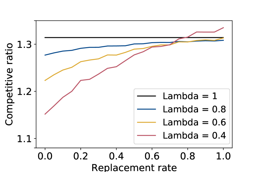
(b) Pareto distribution

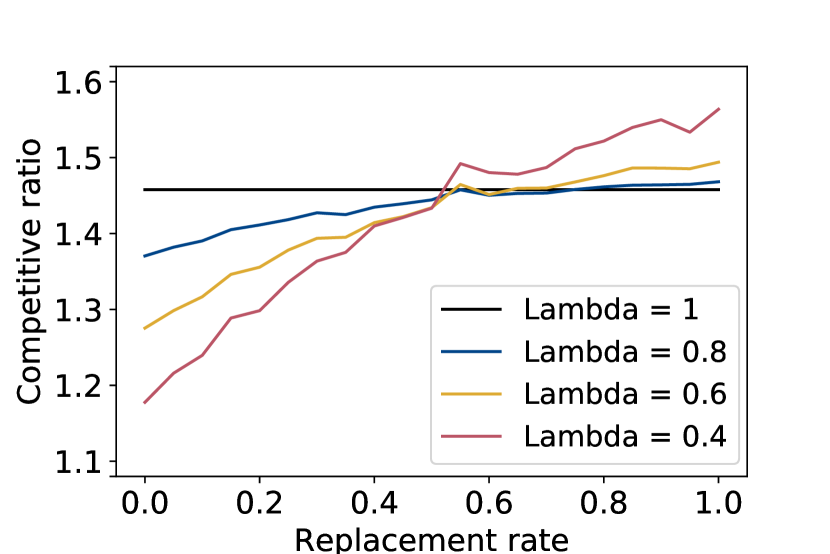
(c) Iterated Poisson distribution

Figure 4: Competitive ratios under various distributions and replacement rates from $0$ to $1$

5 Future Directions

In this paper we present the PDLA technique, a learning augmented version of the classic Primal-Dual technique, and apply it to design algorithms for some classic online problems when a prediction is provided. Since the Primal-Dual technique is used to solve many more covering problems, like for instance weighted caching or load balancing [4], an interesting research direction would be to apply PDLA to tackle those problems and (hopefully) get tight consistency-robustness trade-off guarantees (as the one achieved by Algorithm 4 and proved in Lemma 3). In addition to that, we suspect that this work might provide insights not only for covering but also for some packing problems which are solved using the Primal-Dual technique in the classic online model (e.g. revenue maximization in ad-auctions [5]). Finally, another interesting direction would be to incorporate predictions into the Primal-Dual technique when used to solve covering problems where the objective function is non linear (e.g. convex).

Broader Impact

The field of learning augmented algorithms lies in the intersection of machine learning and online algorithms, trying to combine the best of the two worlds. Learning augmented algorithms are particularly suited for critical applications where maintaining worst-case guarantees is mandatory but at the same time predictions about the future are possible. Thus, our work represents a stepping stone towards (easily) integrating ML predictions in such applications, increasing this way the possible benefits of ML to society. PDLA offers a recipe on how to incorporate predictions to tackle classical covering online problems, that is to first solve the online problem using the Primal-Dual technique and then use the prediction to change the rate at which primal and dual variables increase or decrease. We believe that since the idea behind this technique is simple and does not require too much domain-specific knowledge, it might be applicable to different problems and can also be implemented in practice.

Appendix A Missing proofs for Set Cover

We first present the slightly modified algorithm where we do not need the prediction to form a feasible solution. As mentioned in the main paper, when an element $e$ is uncovered by the prediction, i.e. $|\operatorname{\mathcal{F}}(e)\cap\operatorname{\mathcal{A}}|=0$, we just run the purely online algorithm ($\lambda=1$).

Algorithm 7 PDLA for Online Weighted Set Cover.

  Input: $\lambda$, $\operatorname{\mathcal{A}}$

  Initialize: $x_{S}\leftarrow 0$, $y_{e}\leftarrow 0$ $\forall S,e$

  for all element $e$ that just arrived do

     while $\sum_{S\in\operatorname{\mathcal{F}}(e)}x_{S}<1$ do

        for all $S\in\operatorname{\mathcal{F}}(e)$ do

           if  $|\operatorname{\mathcal{F}}(e)\cap\operatorname{\mathcal{A}}|\geqslant 1$ then

               /* Primal Update (more aggressive if $\mathbbm{1}\{S\in\operatorname{\mathcal{A}}\}=1$ )

              ${x_{S}\leftarrow x_{S}\left(1+\frac{1}{w_{S}}\right)+\frac{\lambda}{w_{S}\cdot|\operatorname{\mathcal{F}}(e)|}+\frac{(1-\lambda)\cdot\mathbbm{1}\{S\in\operatorname{\mathcal{A}}\}}{w_{S}\cdot|\operatorname{\mathcal{F}}(e)\cap\operatorname{\mathcal{A}}|}}$

           else

              /* e is not covered by the prediction

              $x_{S}\leftarrow x_{S}\cdot\left(1+\frac{1}{w_{S}}\right)+\frac{1}{w_{S}\cdot|\operatorname{\mathcal{F}}(e)|}$

           end if

        end for

         /* Dual Update

        $y_{e}\leftarrow y_{e}+1$

     end while

  end for

We start by proving that the dual constraints are only violated by a multiplicative factor of $O\left(\log\left(\frac{d}{\lambda}\right)\right)$. Thus, scaling down the dual solution of Algorithm 7 by $O\left(\log\left(\frac{d}{\lambda}\right)\right)$ creates a feasible dual solution which will permit us to use weak duality.

Lemma 6.

Let $y$ be the dual solution built by Algorithm 7. Then $\frac{y}{\Theta(\log(d/\lambda))}$ is a feasible solution to the dual problem.

Proof.

The proof essentially follows the same path as in [4]. The only constraints that can be violated are of the form $\sum_{e\in S}y_{e}\leqslant w_{S}$ for some $S\in\mathcal{F}$. Consider one such constraint. At every update of the primal variable $x_{S}$ the sum $\sum_{e\in S}y_{e}$ increases by 1, since the dual variable corresponding to the newly arrived element increases by $1$ . We prove by induction on the number of such updates that at any point in time ${x_{S}\geqslant\frac{\lambda}{d}\left(\left(1+\frac{1}{w_{S}}\right)^{\sum_{e\in S}y_{e}}-1\right)}$. Indeed, when no update concerning $S$ is done we have that $x_{S}=0$ and $\sum_{e\in S}y_{e}=0$. Suppose this is true after $k$ updates of the variable $x_{S}$, i.e. $\sum_{e\in S}y_{e}=k$. Now, assume that a newly arrived element $e^{*}\in S$ provokes a primal update from $x_{S}^{\textit{old}}$ to $x_{S}^{\textit{new}}$ and increases its dual value by one, i.e. ${y_{e^{*}}^{\textit{new}}=y_{e^{*}}^{\textit{old}}+1}$. Then we always have:

$$x_{S}^{\textit{new}}\geqslant x_{S}^{\textit{old}}\cdot\left(1+\frac{1}{w_{S}}\right)+\min\left\{\frac{1}{|\operatorname{\mathcal{F}}(e)|\cdot w_{S}},\frac{\lambda}{|\operatorname{\mathcal{F}}(e)|\cdot w_{S}}+\frac{(1-\lambda)\cdot\mathbbm{1}\{S\in\operatorname{\mathcal{A}}\}}{|\operatorname{\mathcal{F}}(e)\cap\operatorname{\mathcal{A}}|\cdot w_{S}}\right\}\geqslant$$

$$\geqslant x_{S}^{\textit{old}}\cdot\left(1+\frac{1}{w_{S}}\right)+\frac{\lambda}{d\cdot w_{S}}$$

Thus, by the induction hypothesis

$$x_{S}^{\textit{new}}\geqslant \frac{\lambda}{d}\left(\left(1+\frac{1}{w_{S}}\right)^{\sum_{e\in S\setminus\{e^{*}\}}y_{e}+y_{e^{*}}^{\textit{old}}}-1\right)\cdot\left(1+\frac{1}{w_{S}}\right)+\frac{\lambda}{d\cdot w_{S}}$$

$$= \frac{\lambda}{d}\left(\left(1+\frac{1}{w_{S}}\right)^{\sum_{e\in S\setminus\{e^{*}\}}y_{e}+y_{e^{*}}^{\textit{new}}}-1\right)=\frac{\lambda}{d}\left(\left(1+\frac{1}{w_{S}}\right)^{\sum_{e\in S}y_{e}}-1\right)$$

Moreover, since $w_{S}\geqslant 1$, we have that $(1+1/w_{s})^{w_{s}}\geqslant 2$, thus:

$$x_{S}\geqslant\frac{\lambda}{d}\left(\left(1+\frac{1}{w_{S}}\right)^{w_{S}\cdot\frac{\sum_{e\in S}y_{e}}{w_{S}}}-1\right)\geqslant\frac{\lambda}{d}\left(2^{\frac{\sum_{e\in S}y_{e}}{w_{S}}}-1\right)$$

We continue by upper bounding the value of $x_{S}$. Note that once $x_{S}\geqslant 1$, no more primal updates can happen, therefore whenever an update is made we have $x_{S}<1$ just before the update. Thus:

$$x_{S}^{\textit{new}} \leqslant x_{S}^{\textit{old}}\cdot\left(1+\frac{1}{w_{S}}\right)+\max\left\{\frac{\lambda}{w_{S}\cdot|\operatorname{\mathcal{F}}(e)|}+\frac{(1-\lambda)\cdot\mathbbm{1}\{S\in\operatorname{\mathcal{A}}\}}{w_{S}\cdot|\operatorname{\mathcal{F}}(e)\cap\operatorname{\mathcal{A}}|},\frac{1}{w_{S}\cdot|\operatorname{\mathcal{F}}(e)|}\right\}$$

$$\leqslant x_{S}^{\textit{old}}\cdot 2+1\leqslant 3$$

Combining the lower and upper bound on $x_{S}$ we get that:

$$\sum_{e\in S}y_{e}\leqslant\log\left(\frac{3d}{\lambda}+1\right)\cdot w_{S}=O(\log\left(d/\lambda\right))\cdot w_{S}$$

which concludes the proof. ∎

Lemma 7 (Robustness).

The competitive ratio is always bounded by $O\left(\log\left(\frac{d}{\lambda}\right)\right)$

Proof.

We denote as before by $x_{S}^{\textit{old}}$ and $x_{S}^{\textit{new}}$ the primal variables before and after the update respectively. Each time the while loop is executed we have that $\sum_{S\in\operatorname{\mathcal{F}}(e)}x_{S}^{\textit{old}}<1$ and the increase in the dual is $\Delta D=1$. Denote by $\delta x_{S}=x_{S}^{\textit{new}}-x_{S}^{\textit{old}}$ the increase of a variable for a specific set $S$. If an element is covered by the prediction then it holds that:

$$\Delta P= \sum_{S\in\operatorname{\mathcal{F}}(e)}w_{S}\cdot\delta x_{S}=\sum_{S\in\operatorname{\mathcal{F}}(e)\cap\operatorname{\mathcal{A}}}w_{S}\cdot\delta x_{S}+\sum_{S\in\operatorname{\mathcal{F}}(e)\setminus\operatorname{\mathcal{F}}(e)\cap\operatorname{\mathcal{A}}}w_{S}\cdot\delta x_{S}=$$

$$= \sum_{S\in\operatorname{\mathcal{F}}(e)}\left(x_{S}^{\textit{old}}+\frac{\lambda}{|\operatorname{\mathcal{F}}(e)|}\right)+\sum_{S\in\operatorname{\mathcal{F}}(e)\cap\operatorname{\mathcal{A}}}\frac{(1-\lambda)}{|\operatorname{\mathcal{F}}(e)\cap\mathcal{A}|}=\sum_{S\in\operatorname{\mathcal{F}}(e)}x_{S}^{\textit{old}}+\lambda+1-\lambda\leqslant 2$$

By repeating the same calculation we get that if an element is uncovered by the prediction then:

$$\Delta P= \sum_{S\in\operatorname{\mathcal{F}}(e)}w_{S}\cdot\delta x_{S}=\sum_{S\in\operatorname{\mathcal{F}}(e)}\left(x_{S}^{\textit{old}}+\frac{1}{|\operatorname{\mathcal{F}}(e)|}\right)=\sum_{S\in\operatorname{\mathcal{F}}(e)}x_{S}^{\textit{old}}+1\leqslant 2$$

Overall we have that:

1. At any iteration $\frac{\Delta P}{\Delta D}\leqslant 2$.

2. The final primal solution is feasible.

3. By Lemma 6, denoting $y$ the final dual solution, $\frac{y}{\Theta(\log(d/\lambda)}$ is feasible.

Thus, by weak duality we get that the competitive ratio of Algorithm 7 is upper bounded by ${2\cdot O(\log\left(d/\lambda\right))}={O(\log\left(d/\lambda\right)))}$. ∎

In the following we do not assume that our prediction $\operatorname{\mathcal{A}}$ forms a feasible solution. Therefore we will denote by

1. $S(\operatorname{\mathcal{A}},\operatorname{\mathcal{I}})$ the cost of the (possibly partial) covering if prediction $\operatorname{\mathcal{A}}$ is followed blindly.

2. $C_{\textit{nc}}$ the cost of optimally covering elements which are not covered by the prediction.

3. $c_{\tiny\mathcal{PDLA}}(\mathcal{A},\mathcal{I},\lambda)$ the cost of the covering solution calculated by Algorithm 7.

Lemma 8 (Consistency).

$c_{\tiny\mathcal{PDLA}}(\mathcal{A},\mathcal{I},\lambda)\leqslant O\left(\frac{1}{1-\lambda}\right)\cdot S(\operatorname{\mathcal{A}},\operatorname{\mathcal{I}})+O(\log\left(d\right))\cdot C_{\textit{nc}}$

Proof.

We split the analysis in two parts. First, we look at the case when an element which is uncovered by the prediction arrives. In this case Algorithm 7 emulates the pure online algorithm ($\lambda=1$). More precisely, by the same calculations as before, we can show that $y_{nc}$ the solution of the dual problem restricted to the uncovered elements satisfy the property that $\frac{y_{nc}}{O(\log d)}$ is feasible. Therefore for those elements by Lemma 7 the cost of Algorithm 7 is upper bounded by $O(\log d)\cdot C_{\textit{nc}}$. We turn our attention to the more interesting case where the prediction covers an element. In this case, after the execution of the while loop we decompose the primal increase into two parts. $\Delta P_{c}$ which denotes the increase due to sets $S$ chosen by $\operatorname{\mathcal{A}}$ ($\mathbbm{1}\{S\in\operatorname{\mathcal{A}}\}=1$) and $\Delta P_{u}$ which denotes the increase due to sets $S$ not chosen by the prediction ($\mathbbm{1}\{S\in\operatorname{\mathcal{A}}\}=0$), thus we have ${\Delta P=\Delta P_{c}+\Delta P_{u}}$. Let $c=\{S\in\operatorname{\mathcal{F}}(e):\mathbbm{1}\{S\in\operatorname{\mathcal{A}}\}=1\}$ and $u=\{S\in\operatorname{\mathcal{F}}(e):\mathbbm{1}\{S\in\operatorname{\mathcal{A}}\}=0\}$. We then have:

$$\Delta P_{c} =\sum_{S\in c}x_{S}+\frac{\lambda\cdot|c|}{|c|+|u|}+1-\lambda\geqslant\frac{\lambda}{d}+1-\lambda$$

$$\Delta P_{u} =\sum_{S\in u}x_{S}+\frac{\lambda\cdot|u|}{|c|+|u|}\leqslant 1+\lambda$$

since , $\frac{|c|}{|c|+|u|}\geqslant\frac{1}{d}$ and $\frac{|u|}{|c|+|u|}\leqslant 1$. Combining the two bounds we get that $\Delta P_{u}\leqslant\frac{1+\lambda}{\frac{\lambda}{d}+1-\lambda}\cdot\Delta P_{c}$ and consequently:

$$\Delta P\leqslant\left(1+\frac{1+\lambda}{\frac{\lambda}{d}+1-\lambda}\right)\Delta P_{c}=O\left(\frac{1}{1-\lambda}\right)\Delta P_{c}$$

Since the cost increase $\Delta P_{c}$ is caused by sets which are selected by the prediction, we can charge this cost to the corresponding increase of $S(\operatorname{\mathcal{A}},\operatorname{\mathcal{I}})$ loosing only a multiplicative $O(1)$ factor. By combining the two cases we conclude the proof. ∎

Appendix B Missing proofs for ski rental and the Bahncard problem

We detail here the missing proofs from section 3. We first prove our results regarding the ski rental problem and then focus on the Bahncard problem.

B.1 The ski rental problem

We provide here a full proof of Theorem 2. In our setting, the prediction $\operatorname{\mathcal{A}}$ is the predicted number of skiing days $N^{\textit{pred}}$ and $S(\operatorname{\mathcal{A}},\operatorname{\mathcal{I}})=S(N^{\textit{pred}},\operatorname{\mathcal{I}})=B\cdot\mathbbm{1}\{N^{\textit{pred}}>B\}+N\cdot\mathbbm{1}\{N^{\textit{pred}}\leqslant B\}$ is the cost of following blindly the prediction. We first prove an easy lemma about the feasibility of the dual solution.

Lemma 9.

Let $y$ be the dual solution built by Algorithm 4. Then $y$ is a feasible solution (assuming $\frac{B}{\lambda}$ is integral if the prediction suggests to rent).

Proof.

To see this, note that the only constraint that might by violated is the constraint $\sum_{j\in[N]}y_{j}\leqslant B$. Denote by $S$ the value of the sum $\sum_{j\in[N]}y_{j}$. Note that once $x\geqslant 1$, the value of $S$ will never change anymore. The value of $S$ increases by $1$ for every big update and by $\lambda$ for every small update. In the case $N^{\textit{pred}}>B$, the algorithm always does big updates (the prediction suggest to buy). We claim that at most $\left\lceil\lambda B\right\rceil$ big updates can be made before $x\geqslant 1$. We denote $x(k)$ the value of $x$ after $k$ updates. We then prove by induction that $x(k)\geqslant\frac{e(k/B)-1}{e(\lambda)-1}$ (recall that $e(z)=(1+1/B)^{z\cdot B}\approx e^{z}$). Clearly, if $k=0$, we have $x(0)\geqslant 0$. Now assume this is the case for $k$ updates we then have

$$x(k+1) =\left(1+\frac{1}{B}\right)\cdot x(k)+\frac{1}{(e(\lambda)-1)\cdot B}$$

$$\geqslant\left(1+\frac{1}{B}\right)\cdot\frac{e(k/B)-1}{e(\lambda)-1}+\frac{1}{(e(\lambda)-1)\cdot B}$$

$$=\frac{\left(1+1/B\right)\cdot(e(k/B)-1)+1/B}{e(\lambda)-1}$$

$$=\frac{e((k+1)/B)-1}{e(\lambda)-1}$$

which ends the induction. Hence at most $\left\lceil\lambda B\right\rceil\leqslant B$ big updates can be made before $x\geqslant 1$. This implies that $S\leqslant B$ at the end of the algorithm. In the case where $N^{\textit{pred}}\leqslant B$, we prove in exactly the same way that at most $\left\lceil\frac{B}{\lambda}\right\rceil$ updates are performed before $x\geqslant 1$. Hence we have that $S\leqslant\lambda\cdot\left\lceil\frac{B}{\lambda}\right\rceil$. By assumption, we have that $B/\lambda$ is an integer hence $S\leqslant 1$ and $y$ is again feasible. ∎

We can finish the main proof.

Proof of Theorem 2.

We prove first the robustness bound. By the Lemma 9, we know that the dual solution is feasible. Hence what remains to prove is to upper bound the ratio $\frac{\Delta P}{\Delta D}$ and use weak duality. In the case of a big update we have

$$\frac{\Delta P}{\Delta D}=\Delta P=1+\frac{1}{e(\lambda)-1}=\frac{1}{1-e(-\lambda)}$$

In the case of a small update we have

$$\frac{\Delta P}{\Delta D}=\frac{\Delta P}{\lambda}=\frac{1}{\lambda}\cdot\frac{1}{1-e(-1/\lambda)}\leqslant\frac{1}{1-e(-\lambda)}$$

where the last inequality comes from Lemma 19 inequality (2). By weak duality, we have the robustness bound.

To prove consistency, we have two cases. If $N^{\textit{pred}}\leqslant B$, then Algorithm 4 does at most $N$ updates, each of cost at most $\frac{1}{1-e(-1/\lambda)}$ while the prediction $\operatorname{\mathcal{A}}$ pays a cost of $N$. Noting again that, by Lemma 19, $\frac{1}{1-e(-1/\lambda)}\leqslant\frac{\lambda}{1-e(-\lambda)}$ ends the proof of consistency in this case. The other case is different. As in the proof of Lemma 9, we still have that $x(k)\geqslant\frac{e(k/B)-1}{e(\lambda)-1}$ hence at most $\left\lceil\lambda B\right\rceil\leqslant B$ updates are done by Algorithm, each of cost at most $\frac{1}{1-e(-\lambda)}$ hence a total cost of at most

$$\frac{\left\lceil\lambda B\right\rceil}{1-e(-\lambda)}$$

Since we assume in this case that $\lambda B$ is integral and that the prediction $\operatorname{\mathcal{A}}$ pays a cost of $B$, the competitive ratio is indeed $\frac{\lambda}{1-e(-\lambda)}$ ∎

B.2 The Bahncard problem

History of the problem.

The Banhcard problem, which was initially introduced in [9], models a situation where a tourist travels every day multiple trips. Before any new trip, the tourist has two choices, either to buy a ticket for that particular trip at a cost of $1$ or buy a discount card, at a cost of $B$, and use this discount card to get a ticket for a price of $\beta<1$. The discount card is then valid for rest of that day and for the next $T-1$ days. This generalizes the ski rental problem in several ways, first the discount expires after a fixed amount of time, second buying only offers a discount and not a free trip. Note that if ${\beta=0}$ and ${T\xrightarrow[]{}\infty}$ we recover the ski-rental problem. Karlin et al. [15] designed an optimal randomized online algorithm of competitive ratio $\frac{e}{e-1+\beta}$ when ${B\xrightarrow[]{}\infty}$.

PDLA for the Bahncard problem.

We design, using PDLA, a learning augmented algorithm for the Bahncard problem. The final goal is to prove Theorem 4. An interesting feature of our algorithm is that, as for the TCP ack problem, it does not need to be given the full prediction in advance. If Bahncards are bought by the prediction $\operatorname{\mathcal{A}}$ at a set of times $\{t_{1},t_{2},\ldots,t_{k}\}$, the algorithm does not need to know before time $t_{i}$ that the Bahncard $i$ is bought. For instance we could think of the prediction of an employee of the station giving short-term advice to a traveller every time he shows up at the station.

We now give the primal dual formulation of the Bahncard problem along with its corresponding learning augmented algorithm. We mention that, to the best of our knowledge, no online algorithm using the primal-dual method was designed before. Hence the primal-dual formulation (Figure 5) of the problem is new. In an integral solution, we would have $x_{t}=1$ if the solution buys a Bahncard at time $t$ and $x_{t}=0$ otherwise. Then $f_{j}$ represents the fractional amount of trip $j$ done at time $t(j)$ that is bought at full price and $d_{j}$ the amount of the trip bought at discounted price. The first natural constraint is the one that says that each trip should be paid entirely either in discounted or full price, i.e. $d_{j}+f_{j}\geqslant 1$. We then have the constraint $\sum_{t=t(j)-T}^{t(j)}x_{t}\geqslant d_{j}$ that says that to be able to buy a ticket at discounted price, at least one Bahncard must have been bought in the last $T$ time steps.

Figure 5: Primal Dual formulation of the Bahncard problem.

Primal	Dual
minimize $B\cdot\sum_{t\in T}x_{t}+\sum_{j\in M}\beta d_{j}+f_{j}$	maximize $\sum_{j\in M}c_{j}$
subject to: $\quad d_{j}+f_{j}\geqslant 1\quad\forall j$	subject to: $\quad c_{j}\leqslant 1\quad\forall j$
$\sum_{t=t(j)-T}^{t(j)}x_{t}\geqslant d_{j}\quad\forall j$	$c_{j}-b_{j}\leqslant\beta\quad\forall j$
$x_{t}\geqslant 0\quad\forall t\in\mathcal{T}$	$\sum_{j:t(j)-T\leqslant t\leqslant t(j)}b_{j}\leqslant B\quad\forall t\in\mathcal{T}$
$d_{j},f_{j}\geqslant 0\quad\forall j$	$c_{j},b_{j}\geqslant 0\quad\forall j$

Following the same idea as for the ski rental problem, we will guide the updates in the primal-dual algorithm with the advice provided. We define a function $e(z)=\left(1+\frac{1-\beta}{B}\right)^{z\cdot(B/(1-\beta))}$. Again for $\frac{B}{1-\beta}\rightarrow\infty$, the reader should think intuitively of $e(z)$ as $e^{z}$. The parameter $z$ will then take values either $\lambda$ or $1/\lambda$ depending on if we want to do a big or small update in the primal. As for ski rental, when we do a small update, we will need to scale down the dual update by a factor of $\lambda$ to maintain feasibility of the dual solution.

The rule to decide if an update should be big or small is the following: if the prediction $\mathcal{A}$ bought a Bahncard less than $T$ time steps in the past (i.e. if the predicted solution has currently a valid Bahncard) the update should be big. Otherwise the update should be cautious. In algorithm 8, we denote by $l_{\mathcal{A}}(t)$ the latest time before time t at which the prediction $\mathcal{A}$ bought a Bahncard. We use the convention that $l_{\mathcal{A}}(t)=-\infty$ if no Bahncard was bought before time $t$. Of course in this problem it is possible that trips show up while the fractional solution already has a full Bahncard available (i.e. $\sum_{t=t(j)-T}^{t(j)}x_{t}\geqslant 1$). In this case there is no point in buying more fractions of a Bahncard and the algorithm will do what we call a minimal update.

Algorithm 8 LA Online Primal-Dual for the Bahncard problem

  Input: $\lambda$, $\mathcal{A}$

  Initialize: $x,d,f\leftarrow 0$, $c,b\leftarrow 0$

  for all trip $j$ do

     if $\sum_{t=t(j)-T}^{t(j)}x_{t}\geqslant 1$ then

        $d_{j}\leftarrow 1$

        $c_{j}\leftarrow\beta$

     end if

     if $\sum_{t=t(j)-T}^{t(j)}x_{t}<1$ then

        if $t(j)\leqslant l_{\mathcal{A}}(t(j))+T$ then

           $d_{j}\leftarrow\sum_{t=t(j)-T}^{t(j)}x_{t}$

           $f_{j}\leftarrow 1-d_{j}$

           $x_{t(j)}\leftarrow x_{t(j)}+\frac{1-\beta}{B}\cdot\left(\sum_{t=t(j)-T}^{t(j)}x_{t}+\frac{1}{e(\lambda)-1}\right)$

           $b_{j}\leftarrow 1-\beta$

           $c_{j}\leftarrow b_{j}+\beta$

        end if

        if $t(j)>l_{\mathcal{A}}(t(j))+T$ then

           $d_{j}\leftarrow\sum_{t=t(j)-T}^{t(j)}x_{t}$

           $f_{j}\leftarrow 1-d_{j}$

           $x_{t(j)}\leftarrow x_{t(j)}+\frac{1-\beta}{B}\cdot\left(\sum_{t=t(j)-T}^{t(j)}x_{t}+\frac{1}{e(1/\lambda)-1}\right)$

           $b_{j}\leftarrow\lambda(1-\beta)$

           $c_{j}\leftarrow b_{j}+\beta$

        end if

     end if

  end for

We first prove that the dual built by the algorithm is almost feasible.

Lemma 10.

Let $(c,b)$ be the dual solution built by Algorithm 8, then $\frac{(c,b)}{1+(1-\beta)/B}$ is feasible.

Proof.

Note that the constraints $c_{j}\leqslant 1$ and $c_{j}-b_{j}\leqslant\beta$ are clearly maintained by the algorithm. And scaling down both $c$ and $b$ by some factor bigger than $1$ will not alter their feasibility. Hence we focus only on the constraints of the form $\sum_{j:t(j)-T\leqslant t\leqslant t(j)}b_{j}\leqslant B$ for a fixed time $t$. Note that during a minimal update, the value of $b_{j}$ is not changed hence only small or big updates can alter the value of the sum $\sum_{j:t(j)-T\leqslant t\leqslant t(j)}b_{j}$. Similarly as for proofs in ski rental, denote by $b$ the number of big updates that are counted in this sum and by $s$ the number of small updates in this sum.

We first notice that once we have that $\sum_{t^{\prime}=t}^{t+T}x_{t^{\prime}}\geqslant 1$, no updates that alter the constraint $\sum_{j:t(j)-T\leqslant t\leqslant t(j)}b_{j}$ can happen. To see this, note that upon arrival of a trip $j$ between time $t$ and $t+T$, we have $\sum_{t=t(j)-T}^{t(j)}x_{t}\geqslant\sum_{t^{\prime}=t}^{t(j)}x_{t^{\prime}}=\sum_{t^{\prime}=t}^{t+T}x_{t^{\prime}}$.

Denote by $S$ the value of the sum $\sum_{t^{\prime}=t}^{t+T}x_{t^{\prime}}$. Note that for a big update, we have that the value of the sum $S$ is increased to at least $S\cdot\left(1+\frac{1-\beta}{B}\right)+\frac{1-\beta}{B}\cdot\frac{1}{e(\lambda)-1}$. Similarly for a small update the new value of the sum is at least $S\cdot\left(1+\frac{1-\beta}{B}\right)+\frac{1-\beta}{B}\cdot\frac{1}{e(1/\lambda)-1}$. Hence we can apply directly Lemma 20 with $d=\frac{B}{1-\beta}$ to conclude that once $b+\lambda s\geqslant\frac{B}{1-\beta}$, we have that $S\geqslant 1$.

Since for a big update, the sum $\sum_{j:t(j)-T\leqslant t\leqslant t(j)}b_{j}$ increases by $1-\beta$ and by $\lambda(1-\beta)$ for a small update we can see that the first time the constraint $\sum_{j:t(j)-T\leqslant t\leqslant t(j)}b_{j}\leqslant B$ is violated, we have $S\geqslant 1$. Now since each update in the sum $\sum_{j:t(j)-T\leqslant t\leqslant t(j)}b_{j}$ is of value at most $1-\beta$ we can conclude that at the end of the algorithm, we have $\sum_{j:t(j)-T\leqslant t\leqslant t(j)}b_{j}\leqslant B+1-\beta$ hence the conclusion. ∎

We then prove robustness of Algorithm 8 by the following lemma.

Lemma 11 (Robustness).

For any $\lambda\in(0,1]$ and any $\beta\in[0,1]$, PDLA for the Bahncard problem is $\frac{\left(e(\lambda)-\beta\right)\cdot\left(1+(1-\beta)/B\right)}{e(\lambda)-1}$-robust.

Proof.

Algorithm 8 makes 3 possible types of updates. For a minimal update, we have $\Delta P=\Delta D=\beta$. For a small update we have

$$\Delta P =\left(1-\beta\right)\cdot\left(\sum_{t=t(j)-T}^{t(j)}x_{t}+\frac{1}{e(1/\lambda)-1}\right)+\beta\cdot\sum_{t=t(j)-T}^{t(j)}x_{t}+1-\sum_{t=t(j)-T}^{t(j)}x_{t}$$

$$=1+\frac{1-\beta}{e(1/\lambda)-1}=\frac{e(1/\lambda)-\beta}{e(1/\lambda)-1}$$

and

$$\Delta D=\lambda(1-\beta)+\beta=\beta(1-\lambda)+\lambda$$

hence the ratio is

$$\frac{\Delta P}{\Delta D}=\frac{1}{\beta(1-\lambda)+\lambda}\cdot\frac{e(1/\lambda)-\beta}{e(1/\lambda)-1}$$

Similarly in the case of a big update we have

$$\Delta P=\frac{e(\lambda)-\beta}{e(\lambda)-1}$$

and $\Delta D=1$ which gives a ratio of

$$\frac{\Delta P}{\Delta D}=\frac{e(\lambda)-\beta}{e(\lambda)-1}$$

We can conclude by Lemma 19 (inequality (7)) that the ratio of primal cost increase vs dual cost increase is always bounded by

$$\frac{\Delta P}{\Delta D}\leqslant\frac{e(\lambda)-\beta}{e(\lambda)-1}$$

Using Lemma 10 along with weak duality is enough to conclude that the cost of the fractional solution built by the algorithm is bounded as follows

$$\textit{cost}_{\tiny{\mathcal{PDLA}}}(\mathcal{A},\mathcal{I},\lambda)\leqslant\frac{\left(e(\lambda)-\beta\right)\cdot\left(1+(1-\beta)/B\right)}{e(\lambda)-1}\cdot\operatorname{OPT}$$

which ends the proof. ∎

For consistency, we analyze the algorithm’s cost in two parts. When the heuristic algorithm $\mathcal{A}$ buys its $i$th Bahncard at some time $t_{i}$, define the interval $I_{i}=[t_{i},t_{i}+T]$ which represents the set of times during which this specific Bahncard is valid. This creates a family of intervals $I_{1},\ldots I_{k}$ if $\mathcal{A}$ buys $k$ Bahncards. Note that we can assume that all these intervals are disjoint since if the prediction $\mathcal{A}$ suggests to buy a new Bahncard before the previous one expires, it is always better to postpone this buy to the end of the validity of the current Bahncard.

Lemma 12.

Denote by $\left(\Delta P\right)_{I_{i}}$ the increase in the primal cost of Algorithm 8 during interval $I_{i}$ and by cost$(\mathcal{A})_{I_{i}}$ what prediction $\mathcal{A}$ pays during this same interval $I_{i}$ (including the buy of the Bahncard at the beginning of the interval $I_{i}$). Then, for all $i$ we have

$$\frac{\left(\Delta P\right)_{I_{i}}}{\mbox{cost}(\mathcal{A})_{I_{i}}}\leqslant\frac{\left\lceil\lambda\cdot\frac{B}{1-\beta}\right\rceil}{B+\beta\cdot\left\lceil\lambda\cdot\frac{B}{1-\beta}\right\rceil}\cdot\frac{e(\lambda)-\beta}{e(\lambda)-1}$$

Proof.

Assume that $m$ trips are requested during this interval $I_{i}$. Then we first have that $cost(\mathcal{A})_{I_{i}}=B+\beta m$ ($\mathcal{A}$ buys a Bahncard then pays a discounted price for every trip in the interval $I_{i}$).

As for Algorithm 8, for each trip $j$, we are possibly in the first two cases: either $\sum_{t=t(j)-T}^{t(j)}x_{t}\geqslant 1$ in which case the increase in the primal is $\Delta P=\beta$ or in the second case in which case the increase in the primal is

$$\Delta P=(1-\beta)\cdot\left(\sum_{t=t(j)-T}^{t(j)}x_{t}+\frac{1}{e(\lambda)-1}\right)+\beta\cdot\sum_{t=t(j)-T}^{t(j)}x_{t}+1-\sum_{t=t(j)-T}^{t(j)}x_{t}=1+\frac{1-\beta}{e(\lambda)-1}$$

We claim that the updates of the second case can happen at most $\left\lceil\lambda\cdot\frac{B}{1-\beta}\right\rceil$ times during interval $I_{i}$. To see this, denote by $S(l)$ the value of $\sum_{t^{\prime}\geqslant t_{i}}x_{t^{\prime}}$ after $l$ big updates in interval $I_{i}$. Note that once $\sum_{t^{\prime}\geqslant t_{i}}x_{t^{\prime}}\geqslant 1$, big updates cannot happen anymore. Hence all we need to prove is that $S\left(\left\lceil\lambda\cdot\frac{B}{1-\beta}\right\rceil\right)\geqslant 1$.

We prove by induction that

$$S(k)\geqslant\frac{e(k\cdot(1-\beta)/B)-1}{e(\lambda)-1}$$

This is indeed true for $k=0$ as $S(0)$ is the value of $\sum_{t^{\prime}\geqslant t_{i}}x_{t^{\prime}}$ before any big update was made in $I_{i}$ hence $S(0)\geqslant 0$. Now assume this is the case for some $k$ and compute

$$S(k+1) \geqslant\left(1+\frac{1-\beta}{B}\right)\cdot S(k)+\frac{1-\beta}{B}\cdot\frac{1}{e(\lambda)-1}$$

$$\geqslant\frac{\left(1+\frac{1-\beta}{B}\right)\cdot\left(e(k\cdot(1-\beta)/B)-1\right)+\frac{1-\beta}{B}}{e(\lambda)-1}$$

$$\geqslant\frac{e((k+1)\cdot(1-\beta)/B)-1}{e(\lambda)-1}$$

which concludes the induction.

Hence on interval $I_{i}$, the total increase in the cost of the solution can be bounded as follows

$$\left(\Delta P\right)_{I_{i}}\leqslant\min\left\{\left\lceil\lambda\cdot\frac{B}{1-\beta}\right\rceil,m\right\}\cdot\left(1+\frac{1-\beta}{e(\lambda)-1}\right)+\max\left\{0,\left(m-\left\lceil\lambda\cdot\frac{B}{1-\beta}\right\rceil\right)\right\}\cdot\beta$$

One can see that the worst case possible for the ratio $\frac{\left(\Delta P\right)_{I_{i}}}{\mbox{cost}(\mathcal{A})_{I_{i}}}$ is obtained for $m=\left\lceil\lambda\cdot\frac{B}{1-\beta}\right\rceil$ and is bounded by

$$\frac{\left(\Delta P\right)_{I_{i}}}{\mbox{cost}(\mathcal{A})_{I_{i}}}\leqslant\frac{\left\lceil\lambda\cdot\frac{B}{1-\beta}\right\rceil\cdot\left(1+\frac{1-\beta}{e(\lambda)-1}\right)}{B+\beta\cdot\left\lceil\lambda\cdot\frac{B}{1-\beta}\right\rceil}=\frac{\left\lceil\lambda\cdot\frac{B}{1-\beta}\right\rceil}{B+\beta\cdot\left\lceil\lambda\cdot\frac{B}{1-\beta}\right\rceil}\cdot\frac{e(\lambda)-\beta}{e(\lambda)-1}$$

∎

We then consider times $t$ that do not belong to any interval $I_{i}$. More precisely, we upper bound the value $\left(\Delta P\right)_{j}$ that is the increase in cost of the primal solution due to trip $j$ such that $t(j)$ does not belong to any interval $I_{i}$. Note that in this case the prediction always pays a cost of $1$.

Lemma 13.

For any trip $j$ such that $t(j)\notin\bigcup_{i}I_{i}$, we have that

$$\left(\Delta P\right)_{j}\leqslant\frac{e(1/\lambda)-\beta}{e(1/\lambda)-1}$$

Proof.

Note that Algorithm 8 pays either the cost of a small update which is $\frac{e(1/\lambda)-\beta}{e(1/\lambda)-1}$ or the cost of a minimal update which is $\beta$. ∎

For simplicity and better readability, we will formulate the final theorem of this section only for $\frac{B}{1-\beta}\rightarrow\infty$.

Theorem (Theorem 4 restated).

For any $\lambda\in(0,1]$, any $\beta\in[0,1]$ and ${\frac{B}{1-\beta}\xrightarrow[]{}\infty}$, we have the following guarantees on any instance $\mathcal{I}$

$$\textit{cost}_{\tiny{\mathcal{PDLA}}}(\mathcal{A},\mathcal{I},\lambda)\leqslant\min\left\{\frac{\lambda}{1-\beta+\lambda\beta}\cdot\frac{e^{\lambda}-\beta}{e^{\lambda}-1}\cdot S(\mathcal{A},I),\frac{e^{\lambda}-\beta}{e^{\lambda}-1}\cdot\operatorname{OPT}\right\}$$

Proof.

By taking the limit in Lemma 11, we see that the cost of the solution output by Algorithm 8 is at most $\frac{e^{\lambda}-\beta}{e^{\lambda}-1}\cdot\operatorname{OPT}$ which proves the second bound in the theorem.

For the first bound, note that we can write the final cost of the solution as

$$\textit{cost}_{\tiny{\mathcal{PDLA}}}(\mathcal{A},\mathcal{I},\lambda)=\Delta P=\sum_{i}\left(\Delta P\right)_{I_{i}}+\sum_{j:t(j)\notin\bigcup_{i}I_{i}}\left(\Delta P\right)_{j}$$

By taking the limit in Lemma 12 we get that

$$\sum_{i}\left(\Delta P\right)_{I_{i}}\leqslant\frac{\lambda}{1-\beta+\beta\lambda}\cdot\frac{e^{\lambda}-\beta}{e^{\lambda}-1}\cdot\sum_{i}\textit{cost}(\mathcal{A})_{I_{i}}$$

and by taking the limit in Lemma 13, we get that

$$\sum_{j:t(j)\notin\bigcup_{i}I_{i}}\left(\Delta P\right)_{j}\leqslant\frac{e^{1/\lambda}-\beta}{e^{1/\lambda}-1}\cdot\sum_{j:t(j)\notin\bigcup_{i}I_{i}}\textit{cost}(\mathcal{A})_{j}$$

By using Lemma 19 (inequality (6)), we see that

$$\max\left\{\frac{\lambda}{1-\beta+\beta\lambda}\cdot\frac{e^{\lambda}-\beta}{e^{\lambda}-1},\frac{e^{1/\lambda}-\beta}{e^{1/\lambda}-1}\right\}=\frac{\lambda}{1-\beta+\beta\lambda}\cdot\frac{e^{\lambda}-\beta}{e^{\lambda}-1}$$

which ends the proof.

∎

We finish this section by proving that a fractional solution can be rounded online into a randomized integral solution. The expected cost of the rounded instance will be equal to the cost of the fractional solution. If the rounding is very similar to the existing rounding of Buchbinder et al. [5] for ski rental or TCP acknowledgement, we still include it here for completeness as the Bahncard problem was never solved in a primal-dual way. The argument is summarized in the following lemma.

Lemma 14.

Given a fractional solution $(x,d,f)$ to the Bahncard problem, it can be rounded online into an integral solution of expected cost equal to the fractional cost of $(x,d,f)$.

Proof.

Choose some real number $p$ uniformly at random in the interval $[0,1]$. Then arrange the variables $x_{t}$ on the real line (i.e. iteratively as follows, each time $t$ takes an interval $I_{t}$ of length $x_{t}$ right after the interval taken by $x_{t-1}$). Then buy a Bahncard at every time $t$ such that the interval corresponding to time $t$ contains the real number $p+k$ for some integer $k$. We check first that the expected buying cost is

$$B\cdot\sum_{t}\mathbbm{E}\left(\mathds{1}_{p+k\in I_{t}}\right)=B\cdot\sum_{t}x_{t}$$

Next, to compute the total expected price of the tickets, notice that if a ticket was bought in the previous $T$ time steps, we can pay a discounted price, otherwise we need to pay the full price of $1$. For a trip $j$, the probability that a ticket was bought in the previous $T$ time steps is at least $\sum_{t=t(j)-T}^{t(j)}x_{t}$. Hence with probability at least $\sum_{t=t(j)-T}^{t(j)}x_{t}\geqslant d_{j}$ we pay a price of $\beta$ and with probability $1-d_{j}\leqslant f_{j}$ we pay a price of $1$ which ends the proof. ∎

Appendix C Missing proofs for TCP

C.1 Plots of instances

We briefly show in Figures 6, 7, and 8 how typical instances under various distributions look like.

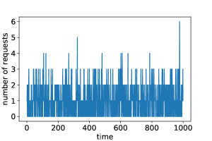
Figure 6: Typical instance under Poisson distribution

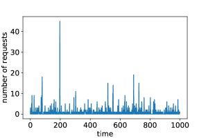
Figure 7: Typical instance under Pareto distribution

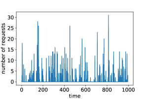
Figure 8: Typical instance under iterated Poisson distribution

C.2 Theoretical analysis

Recall that we define in this section $e(z)=(1+1/d)^{z\cdot d}$ which will be roughly equal to $e^{z}$ for big $d$. The big updates are then the updates where $z$ is set to $\lambda$ and during a small update, $z$ is set to $1/\lambda$.

We first analyze the consistency of this algorithm. To this end denote by $n_{\mathcal{A}}$ the number of acknowledgements sent by $\mathcal{A}$ and by $\textit{latency}\left(\mathcal{A}\right)$ the latency paid by the prediction $\mathcal{A}$.

Lemma 15.

For any $\lambda\in(0,1]$, $d>0$,

$$\textit{c}_{\tiny{\mathcal{PDLA}}}(\mathcal{A},\operatorname{\mathcal{I}},\lambda)\leqslant n_{\mathcal{A}}\cdot\frac{1}{d}\cdot\frac{\left\lceil\lambda d\right\rceil}{1-e(-\lambda)}+\textit{latency}(\mathcal{A})\cdot\frac{1}{1-e(-1/\lambda)}$$

Proof.

We will use a charging argument to analyze the performance of Algorithm 6. Note that for a small update, the increase in cost of the fractional solution is

$$\Delta P=\frac{1}{d}\left(1-\sum_{k=t(j)}^{t}x_{k}\right)+\frac{1}{d}\cdot\left(\sum_{k=t(j)}^{t}x_{k}+\frac{1}{e(1/\lambda)-1}\right)=\frac{1}{d}\cdot\frac{1}{1-e(-1/\lambda)}$$

However, for every small update that is made, it must be that $\mathcal{A}$ pays a latency of at least $\frac{1}{d}$. Hence the total cost of small updates made by Algorithm 6 is at most $\textit{latency}(\mathcal{A})\cdot\frac{1}{1-e(-1/\lambda)}$.

Secondly we bound the total cost of big updates of our algorithm. Let $t_{0}$ be a time at which $\mathcal{A}$ sends an acknowledgment. Let $Y$ be the set of big updates made because of jobs $j$ that are acknowledged at time $t_{0}$ by $\mathcal{A}$ (these big updates are hence made at some time $t\geqslant t_{0}$). We claim that $|Y|\leqslant\left\lceil\lambda d\right\rceil$.

To prove this denote by $S(l)$ the value of $\sum_{k=t_{0}}^{+\infty}x_{k}$ after $l$ such big updates (there might be small updates influencing this value but only to make it bigger). Notice that once $\sum_{k=t_{0}}^{+\infty}x_{k}\geqslant 1$ there is no remaining update in $Y$. We prove by induction that

$$S(l)\geqslant\frac{(1+1/d)^{l}-1}{(1+1/d)^{\lambda d}-1}$$

This is clear for $l=0$ as $S(0)\geqslant 0$. Now assume this is the case for some value $l$ and apply a big update at time $t$ for job $j$ to get

$$S(l+1) =S(l)+\frac{1}{d}\cdot\left(\sum_{k=t(j)}^{t}x_{k}+\frac{1}{e(\lambda)-1}\right)$$

$$\geqslant S(l)\cdot(1+1/d)+\frac{1}{d(e(\lambda)-1)}$$

$$=\frac{(1+1/d)^{l+1}-1-1/d}{(1+1/d)^{\lambda d}-1}+\frac{1/d}{(e(\lambda)-1)}$$

$$=\frac{(1+1/d)^{l+1}-1-1/d}{(1+1/d)^{\lambda d}-1}+\frac{1/d}{(1+1/d)^{\lambda d}-1}$$

$$=\frac{(1+1/d)^{l+1}-1}{(1+1/d)^{\lambda d}-1}$$

Where the second inequality comes from noting that since we are considering an update due to a request $j$ acknowledged at time $t_{0}$ by the predicted solution, it must be that $t(j)\leqslant t_{0}$ and $\sum_{k=t(j)}^{t}x_{k}\geqslant\sum_{k=t_{0}}^{t}x_{k}$. Hence we get that $S\left(\left\lceil\lambda d\right\rceil\right)\geqslant 1$ which implies that $|Y|\leqslant\left\lceil\lambda d\right\rceil$.

By a similar calculation as for the small update case, we have that the cost of a big update is

$$\Delta P=\frac{1}{d}\cdot\frac{1}{1-e(-\lambda)}$$

Hence the total cost of these updates in $Y$ is charged to the acknowledgement that $\mathcal{A}$ pays at time $t_{0}$ to finish the proof. ∎

Taking the limit $d\rightarrow+\infty$ we get the following corollary:

Corollary 16.

For any $\lambda\in(0,1]$ and taking $d\rightarrow+\infty$, we have that

$$\textit{c}_{\tiny{\mathcal{PDLA}}}(\mathcal{A},\operatorname{\mathcal{I}},\lambda)\leqslant n_{\mathcal{A}}\cdot\frac{\lambda}{1-e^{-\lambda}}+\textit{latency}(\mathcal{A})\cdot\frac{1}{1-e^{-1/\lambda}}$$

We then prove robustness of the algorithm with the following lemmas.

Lemma 17.

Let $y$ be the dual solution produced by Algorithm 6. Then $\frac{y}{1+1/d}$ is feasible.

Proof.

Notice that the constraints of the second type (i.e. $0\leqslant y_{jt}\leqslant 1/d$) are always satisfied since $0<\lambda\leqslant 1$. We now check that the second constraints are almost satisfied (within some factor $(1+1/d)$). Fix a time $t\in T$ and consider the corresponding constraint:

$$\sum_{j|t\geqslant t(j)}\sum_{t^{\prime}\geqslant t}y_{jt}\leqslant 1$$

Note that for a small update for some job $j$ such that $t(j)\leqslant t$ the sum above increases by $\lambda/d$ while it increases by $1/d$ for a big update. Notice that once we have that $\sum_{t^{\prime}\geqslant t}x_{t^{\prime}}\geqslant 1$, no more such update will be performed. Denote by $S$ the value of this sum.

Notice that for a big update, the sum $S$ becomes $\left(1+\frac{1}{d}\right)\cdot S+\frac{1}{d((1+1/d)^{\lambda d}-1)}$. Similarly, for a small updates it becomes $\left(1+\frac{1}{d}\right)\cdot S+\frac{1}{d((1+1/d)^{d/\lambda}-1)}$.

Hence, if we denote by $s$ the number of small updates in this sum and by $b$ the number of big updates, by Lemma 20 we have that if $\lambda s+b\geqslant d$ then $\sum_{t^{\prime}\geqslant t}x_{t^{\prime}}\geqslant 1$. This directly implies that the value of $\sum_{j|t\geqslant t(j)}\sum_{t^{\prime}\geqslant t}y_{jt}$ is at most $1+1/d$ at the end of the algorithm (each update in the dual is of value at most $1/d$).

Therefore scaling down all $y_{jt}$ by a multiplicative factor of $1+1/d$ yields a feasible solution to the dual. ∎

Lemma 18.

For $d\rightarrow+\infty$, Algorithm 6 outputs a solution of cost at most $\frac{1}{1-e^{-\lambda}}\cdot\operatorname{OPT}$

Proof.

We first compare the increase $\Delta P$ in the primal value to the increase $\Delta D$ in the dual value at every update. We claim that for every update we have

$$\frac{\Delta P}{\Delta D}\leqslant\frac{1}{1-e(-\lambda)}$$

In the case of a big update we directly have $\Delta P=\frac{1}{d}\left(1+\frac{1}{e(\lambda)-1}\right)=\frac{1}{d}\cdot\frac{1}{1-e(-\lambda)}$ and $\Delta D=\frac{1}{d}$. In the case of a small update we have $\Delta D=\frac{\lambda}{d}$ and $\Delta P=\frac{1}{d}\left(1+\frac{1}{e(1/\lambda)-1}\right)=\frac{1}{d}\cdot\frac{1}{1-e(-1/\lambda)}$ and we conclude applying Lemma 19 (inequality (3)) that we always have

$$\frac{\Delta P}{\Delta D}\leqslant\frac{1}{1-e(-\lambda)}$$

By lemma 17, $\frac{y}{1+1/d}$ is a feasible solution. Hence taking $d\rightarrow+\infty$ together with the previous remark and weak duality we get the result. ∎

Combining Lemma 16 and Lemma 18 yields Theorem 5.

Appendix D Optimality bound

See 3

Proof.

For simplicity, we will consider the ski-rental problem in the continuous case which corresponds to the behaviour of the discrete version when $B\xrightarrow[]{}\infty$. In this problem, the cost of buying is $1$ and a randomized algorithm has to define a (buying) probability distribution $\{p_{t}\}_{t\geqslant 0}$. Moreover, consider the case where the true number of vacation days $t_{\textit{end}}\in[0,1]\cup(2,\infty)$. In such a case we can assume w.l.o.g. that $p_{t}=0,\forall t>1$. Indeed moving buying probability mass from any $p_{t},t>1$ to $p_{1}$ does not increase the cost of the randomized algorithm. Assume now that the prediction suggests us that the end of vacations is at $\hat{t}_{\textit{end}}>2$, thus the optimal offline solution, if the prediction is correct, is to buy the skis in the beginning for a total cost of $1$. Since the algorithm has to define a probability distribution in $[0,1]$, $\{p_{t}\}$ needs to satisfy the equality constraint $\int_{0}^{1}p_{t}dt=1$. Moreover, note that when the prediction is correct, i.e. $t_{\textit{end}}>2$, the LA algorithm suffers an expected cost of $\int_{0}^{1}(t+1)p_{t}dt$ while the optimum offline has a cost of $1$. Thus the consistency requirement forces the distribution to satisfy the inequality $\int_{0}^{1}(t+1)p_{t}dt\leqslant\frac{\lambda}{1-e^{-\lambda}}$. Now assume that the best possible LA algorithm is $c$-robust. If $t_{\textit{end}}\leqslant 1$ then the LA algorithm’s cost is ${\int_{0}^{t_{\textit{end}}}(t+1)p_{t}dt+t_{\textit{end}}\int_{t_{\textit{end}}}^{1}p_{t}dt}$ while the optimum offline cost is $t_{\textit{end}}$. Thus, due to $c$-robustness we have that for every $t^{\prime}\in[0,1]$, ${\int_{0}^{t^{\prime}}(t+1)p_{t}dt+t^{\prime}\int_{t^{\prime}}^{1}p_{t}dt\leqslant ct^{\prime}}$. We calculate the best possible robustness $c$ with the following LP:

Figure 9: Primal Robustness for ski-rental problem.

Primal
minimize $c$
subject to: $\quad\int_{0}^{1}p_{t}dt=1$
$\quad\int_{0}^{1}(t+1)p_{t}dt\leqslant\frac{\lambda}{1-e^{-\lambda}}$
$\quad{\int_{0}^{t^{\prime}}(t+1)p_{t}dt+t^{\prime}\int_{t^{\prime}}^{1}p_{t}dt\leqslant ct^{\prime}}\quad\forall t^{\prime}\in[0,1]$
$\quad p_{t}\geqslant 0\quad\forall t^{\prime}\in[0,1]$

To lower bound the best possible robustness $c$ we will present a feasible solution to the dual of 9. The dual variables $\lambda_{d}$ and $\lambda_{c}$ correspond respectively to the first and second primal constraints in Figure 9. The dual variables $\lambda_{t}$, $\forall t\in[0,1]$ correspond to the robustness constraints described in the third line of the primal.

The corresponding dual is:

Figure 10: Dual Robustness for ski-rental problem.

Dual
maximize $\lambda_{d}-\lambda_{c}\cdot\frac{\lambda}{1-e^{-\lambda}}$
subject to: $\quad\int_{0}^{1}t\lambda_{t}dt\leqslant 1$
$\quad\lambda_{d}-(t^{\prime}+1)\lambda_{c}\leqslant\int_{0}^{t^{\prime}}t\lambda_{t}dt+(t^{\prime}+1)\int_{t^{\prime}}^{1}\lambda_{t}dt\quad\forall t^{\prime}\in[0,1]$
$\lambda_{c},\lambda_{t}\geqslant 0\quad\forall t\in[0,1]$

Let $K=\frac{1}{1-\lambda e^{-\lambda}-e^{-\lambda}}$. Then, $\lambda_{t}=K\cdot e^{-t}\cdot\mathbbm{1}\{t\leqslant\lambda\}$ , $\lambda_{d}=K$ and $\lambda_{c}=K\cdot e^{-\lambda}$.

We first prove that this dual solution is feasible. For the first constraint notice that

$$\int_{0}^{1}t\lambda_{t}dt=K\cdot\int_{0}^{\lambda}te^{-t}dt=K\cdot\left(1-(\lambda+1)e^{-\lambda}\right)=1$$

For the second type of constraint first in the case $t^{\prime}>\lambda$ we get

$$\int_{0}^{t^{\prime}}t\lambda_{t}dt+(t^{\prime}+1)\int_{t^{\prime}}^{1}\lambda_{t}dt=\int_{0}^{\lambda}t\lambda_{t}dt=1$$

and we note that

$$\lambda_{d}-(t^{\prime}+1)\lambda_{c}\leqslant\lambda_{d}-(\lambda+1)\lambda_{c}=K\cdot\left(1-(\lambda+1)e^{-\lambda}\right)=1$$

hence these constraints are satisfied.

In the second case $t^{\prime}\leqslant\lambda$, we have that

$$\int_{0}^{t^{\prime}}t\lambda_{t}dt+(t^{\prime}+1)\int_{t^{\prime}}^{1}\lambda_{t}dt =K\cdot\left(\int_{0}^{t^{\prime}}te^{-t}dt+(t^{\prime}+1)\int_{t^{\prime}}^{\lambda}e^{-t}dt\right)$$

$$=K\cdot\left(1-(t^{\prime}+1)e^{-t^{\prime}}+(t^{\prime}+1)(e^{-t^{\prime}}-e^{-\lambda})\right)$$

$$=K\cdot\left(1-(t^{\prime}+1)e^{-\lambda}\right)$$

$$=\lambda_{d}-(t^{\prime}+1)\lambda_{c}$$

which proves that these constraints are also satisfied. Hence this dual solution is feasible. Finally note that the cost of this dual solution is

$$\lambda_{d}-\lambda_{c}\cdot\frac{\lambda}{1-e^{-\lambda}} =K\cdot\left(1-\frac{\lambda}{1-e^{-\lambda}}\cdot e^{-\lambda}\right)$$

$$=K\cdot\frac{1-e^{-\lambda}-\lambda e^{-\lambda}}{1-e^{-\lambda}}=\frac{1}{1-e^{-\lambda}}$$

By weak duality, we conclude that the best robustness cannot be better than $\frac{1}{1-e^{-\lambda}}$ ∎

Appendix E Technical lemmas

A few inequalities that will be useful:

Lemma 19.

For any $d>0$, any $0<\lambda\leqslant 1$, and any $\beta\in[0,1]$, we have:

$$\frac{\lambda}{1-e^{-\lambda}}\geqslant\frac{1}{1-e^{-1/\lambda}}$$ (2)

$$\frac{\lambda}{1-(1+1/d)^{-\lambda d}}\geqslant\frac{1}{1-(1+1/d)^{-d/\lambda}}$$ (3)

$$\frac{1}{e^{\lambda}-1}\geqslant\frac{\frac{1-\lambda}{\lambda}\cdot e^{1/\lambda}+1}{e^{1/\lambda}-1}$$ (4)

$$\frac{1}{(1+1/d)^{\lambda d}-1}\geqslant\frac{\frac{1-\lambda}{\lambda}\cdot(1+1/d)^{d/\lambda}+1}{(1+1/d)^{d/\lambda}-1}$$ (5)

$$\frac{\lambda}{1-\beta+\beta\lambda}\cdot\frac{e^{\lambda}-\beta}{e^{\lambda}-1}\geqslant\frac{e^{1/\lambda}-\beta}{e^{1/\lambda}-1}$$ (6)

$$(\lambda+\beta-\beta\lambda)\cdot\frac{e^{\lambda}-\beta}{e^{\lambda}-1}\geqslant\frac{e^{1/\lambda}-\beta}{e^{1/\lambda}-1}$$ (7)

Proof.

Since the formal proof of (2) and (4) seems to require heavy calculations and that they are easy to check on computer we will only give a proof by a plot (see Figures 11(a) and 11(b)). For 11(b), note that $\eqref{eqn:lemma12_2b}\iff\frac{1}{e^{\lambda}-1}-\frac{1-\lambda}{\lambda}-\frac{1}{\lambda}\cdot\frac{e^{-1/\lambda}}{1-e^{-1/\lambda}}\geqslant 0$.

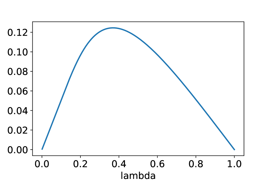
(a) Plot of $\frac{\lambda}{1-e^{-\lambda}}-\frac{1}{1-e^{-1/\lambda}}$

(b) Plot of $\frac{1}{e^{\lambda}-1}-\frac{1-\lambda}{\lambda}-\frac{1}{\lambda}\cdot\frac{e^{-1/\lambda}}{1-e^{-1/\lambda}}$

Figure 11: Plots for (2) and (4)

We now prove that inequality (2) implies inequality (3). For this end notice that we can write $(1+1/d)^{d}=e^{x}$ for some $x\in(0,1)$ since $(1+1/d)^{d}\in(1,e)$ for all $d>0$. We prove that for any $x\in(0,1]$

$$\frac{\lambda\left(1-e^{-x/\lambda}\right)}{1-e^{-x\lambda}}\geqslant\frac{\lambda\left(1-e^{-1/\lambda}\right)}{1-e^{-\lambda}}$$

which will imply our claim since by inequality (2) the right hand side is bigger than $1$. First note this is equivalent to prove that

$$g_{\lambda}(x)=(1-e^{-\lambda})\cdot(1-e^{-x/\lambda})-(1-e^{-1/\lambda})\cdot(1-e^{-x\lambda})\geqslant 0$$

Taking the derivative of $g_{\lambda}(x)$ we obtain

$$g^{\prime}_{\lambda}(x)=\frac{1-e^{-\lambda}}{\lambda}\cdot e^{-x/\lambda}-\lambda(1-e^{-1/\lambda})\cdot e^{-x\lambda}$$

hence we can write

$$g^{\prime}_{\lambda}(x)\geqslant 0\iff e^{x\left(\lambda-1/\lambda\right)}\geqslant\lambda^{2}\cdot\frac{1-e^{-1/\lambda}}{1-e^{-\lambda}}$$

Notice that the left hand side in this inequality is decreasing because $\lambda\in(0,1]$. Also notice that $g_{\lambda}(0)=g_{\lambda}(1)=0$. These two facts together imply that $g_{\lambda}$ is first increasing for $x\in(0,c]$ then decreasing for $x\in(c,1]$ for some unknown $c$. In particular, we indeed have that $g_{\lambda}(x)\geqslant 0$ which ends the proof of inequality (3).

Similarly, we prove that inequality (4) implies inequality (5). Again we write $(1+1/d)^{d}=e^{x}$ for some $x\in(0,1)$. We first rewrite inequality (5).

$$\eqref{eqn:lemma12_2} \iff\frac{1}{e^{\lambda x}-1}\geqslant\frac{\frac{1-\lambda}{\lambda}\cdot e^{x/\lambda}+1}{e^{x/\lambda}-1}$$

$$\iff\frac{1}{e^{\lambda x}-1}\geqslant\frac{\frac{1-\lambda}{\lambda}\cdot(e^{x/\lambda}-1)+\frac{1}{\lambda}}{e^{x/\lambda}-1}$$

$$\iff\lambda(e^{x/\lambda}-1)\geqslant(1-\lambda)(e^{x/\lambda}-1)(e^{\lambda x}-1)+(e^{\lambda x}-1)$$

$$\iff\lambda(e^{x/\lambda}-1)-(1-\lambda)(e^{x/\lambda}-1)(e^{\lambda x}-1)-(e^{\lambda x}-1)\geqslant 0$$

Define the following function $h_{\lambda}(x)=\lambda(e^{x/\lambda}-1)-(1-\lambda)(e^{x/\lambda}-1)(e^{\lambda x}-1)-(e^{\lambda x}-1)$. One can first compute:

$$h^{\prime}_{\lambda}(x) =e^{x/\lambda}-(1-\lambda)\cdot\left(\lambda e^{\lambda x}(e^{x/\lambda}-1)+\frac{1}{\lambda}e^{x/\lambda}(e^{\lambda x}-1)\right)-\lambda e^{\lambda x}$$

$$=e^{x/\lambda}-\lambda e^{\lambda x}-(1-\lambda)\cdot\left((\lambda+1/\lambda)e^{x(\lambda+1/\lambda)}-\lambda e^{\lambda x}-\frac{1}{\lambda}e^{x/\lambda}\right)$$

$$=e^{x/\lambda}\cdot\left(1+\frac{1-\lambda}{\lambda}\right)+e^{\lambda x}\cdot\left(-\lambda+\lambda(1-\lambda)\right)-e^{x(\lambda+1/\lambda)}\cdot(1-\lambda)\cdot\left(\lambda+\frac{1}{\lambda}\right)$$

$$=\frac{e^{x/\lambda}}{\lambda}-\lambda^{2}e^{\lambda x}-\frac{e^{x(\lambda+1/\lambda)}}{\lambda}\cdot(1-\lambda)\cdot(\lambda^{2}+1)$$

Hence we can rewrite

$$h^{\prime}_{\lambda}(x)\geqslant 0 \iff\frac{e^{x/\lambda}}{\lambda}-\lambda^{2}e^{\lambda x}-\frac{e^{x(\lambda+1/\lambda)}}{\lambda}\cdot(1-\lambda)\cdot(\lambda^{2}+1)\geqslant 0$$

$$\iff e^{x/\lambda}-\lambda^{3}e^{\lambda x}-e^{x(\lambda+1/\lambda)}\cdot(1-\lambda)\cdot(\lambda^{2}+1)\geqslant 0$$

$$\iff 1-\lambda^{3}e^{x(\lambda-1/\lambda)}-e^{x\lambda}\cdot(1-\lambda)\cdot(\lambda^{2}+1)\geqslant 0$$

Let us define $i_{\lambda}(x)=1-\lambda^{3}e^{x(\lambda-1/\lambda)}-e^{x\lambda}\cdot(1-\lambda)\cdot(\lambda^{2}+1)$ and we derive

$$i^{\prime}_{\lambda}(x)=-\lambda^{3}\cdot(\lambda-1/\lambda)\cdot e^{x(\lambda-1/\lambda)}-\lambda e^{\lambda x}\cdot(1-\lambda)\cdot(\lambda^{2}+1)$$

We can now notice that

$$i^{\prime}_{\lambda}(x)\geqslant 0 \iff-\lambda^{3}\cdot(\lambda-1/\lambda)\cdot e^{x(\lambda-1/\lambda)}-\lambda e^{\lambda x}\cdot(1-\lambda)\cdot(\lambda^{2}+1)\geqslant 0$$

$$\iff-\lambda^{3}\cdot(\lambda-1/\lambda)\cdot e^{-x/\lambda}-\lambda(1-\lambda)\cdot(\lambda^{2}+1)\geqslant 0$$

$$\iff\lambda^{3}\cdot(1/\lambda-\lambda)\cdot e^{-x/\lambda}-\lambda(1-\lambda)\cdot(\lambda^{2}+1)\geqslant 0$$

Since the left hand side is decreasing as $x$ increases we only need to check one extreme value which is $i^{\prime}_{\lambda}(0)$. We write

$$i^{\prime}_{\lambda}(0)\leqslant 0 \iff\lambda^{3}\cdot(1/\lambda-\lambda)-\lambda\cdot(1-\lambda)\cdot(\lambda^{2}+1)\leqslant 0$$

$$\iff\lambda^{2}-\lambda^{4}-(\lambda^{3}+\lambda-\lambda^{4}-\lambda^{2})\leqslant 0$$

$$\iff-\lambda^{3}+2\lambda^{2}-\lambda\leqslant 0$$

$$\iff-\lambda\cdot(\lambda-1)^{2}\leqslant 0$$

hence we always have $i^{\prime}_{\lambda}(0)\leqslant 0$.

Therefore we get that $i^{\prime}_{\lambda}(x)\leqslant 0$ for all $x$ and $\lambda$. Note that $i_{\lambda}(0)=1-\lambda^{3}-(1-\lambda)(\lambda^{2}+1)=1-\lambda^{3}-\lambda^{2}-1+\lambda^{3}+\lambda=\lambda-\lambda^{2}\geqslant 0$. Therefore we get that $h_{\lambda}$ is first positive on some interval $[0,c]$ and then negative for $x\in[c,\infty)$. Therefore $h_{\lambda}$ is first increasing then decreasing. Notice that $h_{\lambda}(0)=0$ and $h_{\lambda}(1)\geqslant 0$ by inequality (4). Hence inequality (5) is true for all $x\in[0,1]$ which concludes the proof.

Finally, the proof of (6) and (7) are quicker and similar. Note that

$$\eqref{eqn:lemma12_3}\iff\lambda\cdot\frac{e^{\lambda}-\beta}{e^{\lambda}-1}\geqslant(1-\beta+\beta\lambda)\cdot\frac{e^{1/\lambda}-\beta}{e^{1/\lambda}-1}$$

which is equivalent to a polynomial (in $\beta$) of degree $2$ being positive. The leading coefficient of this polynomial $P$ is negative and we notice that $P(1)=0$ and that $P(0)\geqslant 0$ by (2). All these facts together imply that $P(\beta)\geqslant 0$ for all $\beta\in[0,1]$. The proof of (7) is similar. ∎

Lemma 20.

Let $0<\lambda\leqslant 1$, $d>0$ and define the following functions ($x\in\mathbb{R}$):

$$f(x)=\left(1+\frac{1}{d}\right)\cdot x+\frac{1}{d\left((1+1/d)^{\lambda d}-1\right)}$$

$$g(x)=\left(1+\frac{1}{d}\right)\cdot x+\frac{1}{d\left((1+1/d)^{d/\lambda}-1\right)}$$

Given $S\geqslant 0$ and a word $w\in\{a,b\}^{*}$ we define a sequence $S_{w}$ recursively as follows:

$$S_{w.y}=\left\{\begin{array}[]{lll}S\mbox{ if }w.y=\varepsilon\\ f(S_{w})\mbox{ if }y=a\\ g(S_{w})\mbox{ if }y=b\\ \end{array}\right.$$

Then for any $w\in\{a,b\}^{*}$ such that $|w|_{a}+\lambda|w|_{b}\geqslant d$ we have that $S_{w}\geqslant 1$.

Proof.

Let $w^{\prime}=b\ldots ba\ldots a=b^{|w|_{b}}a^{|w|_{a}}$ be the word made of $|w|_{b}$ consecutive $b$s followed by $|w|_{a}$ consecutive $a$s. Then we claim that $S_{w^{\prime}}\leqslant S_{w}$. This directly follows from the fact that for any real number $x$, $f(g(x))\leqslant g(f(x))$. Noticing this, we can swap positions between an $a$ followed by a $b$ and reducing the final value. We keep doing this until all the $b$s in $w$ end up in front position.

With standard computations one can check that

$$S_{b^{|w|_{b}}}=S\cdot\left(1+1/d\right)^{|w|_{b}}+\frac{\left(1+1/d\right)^{|w|_{b}}-1}{(1+1/d)^{d/\lambda}-1}$$

For ease of notation define $S^{\prime}=S_{b^{|w|_{b}}}$. Using the assumption that $|w|_{a}+\lambda|w|_{b}\geqslant d$ and that $S\geqslant 0$ we get that

$$S^{\prime}\geqslant\frac{(1+1/d)^{(d-|w|_{a})/\lambda}-1}{(1+1/d)^{d/\lambda}-1}$$

Again using standard calculations we get that

$$S_{w^{\prime}}\geqslant S^{\prime}\cdot(1+1/d)^{|w|_{a}}+\frac{(1+1/d)^{|w|_{a}}-1}{(1+1/d)^{\lambda d}-1}$$

which implies

$$S_{w^{\prime}}\geqslant\frac{(1+1/d)^{(d-|w|_{a})/\lambda}-1}{(1+1/d)^{d/\lambda}-1}\cdot(1+1/d)^{|w|_{a}}+\frac{(1+1/d)^{|w|_{a}}-1}{(1+1/d)^{\lambda d}-1}$$

Define $h(x)=\frac{(1+1/d)^{(d-x)/\lambda}-1}{(1+1/d)^{d/\lambda}-1}\cdot(1+1/d)^{x}+\frac{(1+1/d)^{x}-1}{(1+1/d)^{\lambda d}-1}$. We finish the proof by proving that for any $0<\lambda\leqslant 1$, any $d>0$ and any $x\geqslant 0$, we have that $h(x)\geqslant 1$.

Note that $h(0)=1$ and that

$$h^{\prime}(x)=\ln(1+1/d)\cdot\left(\frac{(1+1/d)^{x}}{(1+1/d)^{\lambda d}-1}-\frac{1-\lambda}{\lambda}\cdot\frac{(1+1/d)^{(d-(1-\lambda)x)/\lambda}}{(1+1/d)^{d/\lambda}-1}-\frac{(1+1/d)^{x}}{(1+1/d)^{d/\lambda}-1}\right)$$

To study the sign of $h^{\prime}(x)$ we can drop the $\ln(1+1/d)$ and write

$$h^{\prime}(x)\geqslant 0\iff \frac{(1+1/d)^{x}}{(1+1/d)^{\lambda d}-1}-\frac{1-\lambda}{\lambda}\cdot\frac{(1+1/d)^{(d-(1-\lambda)x)/\lambda}}{(1+1/d)^{d/\lambda}-1}-\frac{(1+1/d)^{x}}{(1+1/d)^{d/\lambda}-1}\geqslant 0$$

$$\iff \frac{1}{(1+1/d)^{\lambda d}-1}-\frac{1-\lambda}{\lambda}\cdot\frac{(1+1/d)^{(d-x)/\lambda}}{(1+1/d)^{d/\lambda}-1}-\frac{1}{(1+1/d)^{d/\lambda}-1}\geqslant 0$$

Clearly the last term is increasing as $x$ increases hence we can limit ourselves to prove that $h^{\prime}(0)\geqslant 0$ which we can rewrite

$$h^{\prime}(0)\geqslant 0\iff \frac{1}{(1+1/d)^{\lambda d}-1}-\frac{1-\lambda}{\lambda}\cdot\frac{(1+1/d)^{d/\lambda}}{(1+1/d)^{d/\lambda}-1}-\frac{1}{(1+1/d)^{d/\lambda}-1}\geqslant 0$$

$$\iff \frac{1}{(1+1/d)^{\lambda d}-1}\geqslant\frac{\frac{1-\lambda}{\lambda}\cdot(1+1/d)^{d/\lambda}+1}{(1+1/d)^{d/\lambda}-1}$$

Which holds by equation (5) of Lemma 19. ∎

References

- Alon et al. [2003] Noga Alon, Baruch Awerbuch, and Yossi Azar. The online set cover problem. In Proceedings of the Thirty-Fifth Annual ACM Symposium on Theory of Computing, STOC ’03, page 100–105, New York, NY, USA, 2003. Association for Computing Machinery. ISBN 1581136749. doi: 10.1145/780542.780558. URL https://doi.org/10.1145/780542.780558.
- Antoniadis et al. [2020] Antonios Antoniadis, Christian Coester, Marek Elias, Adam Polak, and Bertrand Simon. Online metric algorithms with untrusted predictions, 2020.
- Bansal et al. [2007] N. Bansal, N. Buchbinder, and J. Naor. A primal-dual randomized algorithm for weighted paging. In 48th Annual IEEE Symposium on Foundations of Computer Science (FOCS’07), pages 507–517, 2007.
- Buchbinder and [Seffi] Niv Buchbinder and Joseph (Seffi) Naor. The design of competitive online algorithms via a primal: Dual approach. Found. Trends Theor. Comput. Sci., 3(2–3):93–263, February 2009. ISSN 1551-305X. doi: 10.1561/0400000024. URL https://doi.org/10.1561/0400000024.
- Buchbinder et al. [2007] Niv Buchbinder, Kamal Jain, and Joseph (Seffi) Naor. Online primal-dual algorithms for maximizing ad-auctions revenue. In Lars Arge, Michael Hoffmann, and Emo Welzl, editors, Algorithms – ESA 2007, pages 253–264, Berlin, Heidelberg, 2007. Springer Berlin Heidelberg.
- Cho et al. [2011] Eunjoon Cho, Seth A. Myers, and Jure Leskovec. Friendship and mobility: User movement in location-based social networks. In Proceedings of the 17th ACM SIGKDD International Conference on Knowledge Discovery and Data Mining, KDD ’11, page 1082–1090, New York, NY, USA, 2011. Association for Computing Machinery. ISBN 9781450308137. doi: 10.1145/2020408.2020579. URL https://doi.org/10.1145/2020408.2020579.
- Dong et al. [2020] Yihe Dong, Piotr Indyk, Ilya Razenshteyn, and Tal Wagner. Learning space partitions for nearest neighbor search. In Eighth International Conference on Learning Representations (ICLR), April 2020. URL https://www.microsoft.com/en-us/research/publication/learning-space-partitions-for-nearest-neighbor-search/.
- Dooly et al. [1998] Daniel R Dooly, Sally A Goldman, and Stephen D Scott. Tcp dynamic acknowledgment delay (extended abstract) theory and practice. In Proceedings of the thirtieth annual ACM symposium on Theory of computing, pages 389–398, 1998.
- Fleischer [2001] Rudolf Fleischer. On the bahncard problem. Theoretical Computer Science, 268(1):161 – 174, 2001. ISSN 0304-3975. doi: https://doi.org/10.1016/S0304-3975(00)00266-8. URL http://www.sciencedirect.com/science/article/pii/S0304397500002668. On-line Algorithms ’98.
- Gollapudi and Panigrahi [2019] Sreenivas Gollapudi and Debmalya Panigrahi. Online algorithms for rent-or-buy with expert advice. In Kamalika Chaudhuri and Ruslan Salakhutdinov, editors, Proceedings of the 36th International Conference on Machine Learning, volume 97 of Proceedings of Machine Learning Research, pages 2319–2327, Long Beach, California, USA, 09–15 Jun 2019. PMLR. URL http://proceedings.mlr.press/v97/gollapudi19a.html.
- Gong et al. [2001] Weibo Gong, Yong Liu, Vishal Misra, and Don Towsley. On the tails of web file size distributions. In in: Proceedings of 39th Allerton Conference on Communication, Control, and Computing, 2001.
- Hsu et al. [2019] Chen-Yu Hsu, Piotr Indyk, Dina Katabi, and Ali Vakilian. Learning-based frequency estimation algorithms. In 7th International Conference on Learning Representations, ICLR 2019, New Orleans, LA, USA, May 6-9, 2019, 2019. URL https://openreview.net/forum?id=r1lohoCqY7.
- Karlin et al. [1986] A. R. Karlin, M. S. Manasse, L. Rudolph, and D. D. Sleator. Competitive snoopy caching. In 27th Annual Symposium on Foundations of Computer Science (sfcs 1986), pages 244–254, 1986.
- Karlin et al. [1990] Anna R. Karlin, Mark S. Manasse, Lyle A. McGeoch, and Susan Owicki. Competitive randomized algorithms for non-uniform problems. In Proceedings of the First Annual ACM-SIAM Symposium on Discrete Algorithms, SODA ’90, page 301–309, USA, 1990. Society for Industrial and Applied Mathematics. ISBN 0898712513.
- Karlin et al. [2001] Anna R. Karlin, Claire Kenyon, and Dana Randall. Dynamic tcp acknowledgement and other stories about e/(e-1). In Proceedings of the Thirty-Third Annual ACM Symposium on Theory of Computing, STOC ’01, page 502–509, New York, NY, USA, 2001. Association for Computing Machinery. ISBN 1581133499. doi: 10.1145/380752.380845. URL https://doi.org/10.1145/380752.380845.
- Kodialam [2019] Rohan Kodialam. Optimal algorithms for ski rental with soft machine-learned predictions. CoRR, abs/1903.00092, 2019. URL http://arxiv.org/abs/1903.00092.
- Lattanzi et al. [2020] Silvio Lattanzi, Thomas Lavastida, Benjamin Moseley, and Sergei Vassilvitskii. Online scheduling via learned weights. In Proceedings of the 2020 ACM-SIAM Symposium on Discrete Algorithms, SODA 2020, Salt Lake City, UT, USA, January 5-8, 2020, pages 1859–1877, 2020. doi: 10.1137/1.9781611975994.114. URL https://doi.org/10.1137/1.9781611975994.114.
- Lee et al. [2019] Russell Lee, Mohammad H. Hajiesmaili, and Jian Li. Learning-assisted competitive algorithms for peak-aware energy scheduling. CoRR, abs/1911.07972, 2019. URL http://arxiv.org/abs/1911.07972.
- Lykouris and Vassilvitskii [2018] Thodoris Lykouris and Sergei Vassilvitskii. Competitive caching with machine learned advice. In Proceedings of the 35th International Conference on Machine Learning, ICML 2018, Stockholmsmässan, Stockholm, Sweden, July 10-15, 2018, pages 3302–3311, 2018. URL http://proceedings.mlr.press/v80/lykouris18a.html.
- Marathe and Hawe [1982] M. Marathe and W. Hawe. Predicted capacity of ethernet in a university environment. In Proceedings of Southcon 1982, pages 1–10, 1982.
- Medina and Vassilvitskii [2017] Andres Muñoz Medina and Sergei Vassilvitskii. Revenue optimization with approximate bid predictions. In Advances in Neural Information Processing Systems 30: Annual Conference on Neural Information Processing Systems 2017, 4-9 December 2017, Long Beach, CA, USA, pages 1858–1866, 2017. URL http://papers.nips.cc/paper/6782-revenue-optimization-with-approximate-bid-predictions.
- Mitzenmacher [2003] Michael Mitzenmacher. Dynamic models for file sizes and double pareto distributions. Internet Math., 1(3):305–333, 2003. URL https://projecteuclid.org:443/euclid.im/1109190964.
- Mitzenmacher [2018] Michael Mitzenmacher. A model for learned bloom filters and optimizing by sandwiching. In S. Bengio, H. Wallach, H. Larochelle, K. Grauman, N. Cesa-Bianchi, and R. Garnett, editors, Advances in Neural Information Processing Systems 31, pages 464–473. Curran Associates, Inc., 2018. URL http://papers.nips.cc/paper/7328-a-model-for-learned-bloom-filters-and-optimizing-by-sandwiching.pdf.
- Mitzenmacher [2019] Michael Mitzenmacher. Scheduling with Predictions and the Price of Misprediction. arXiv e-prints, art. arXiv:1902.00732, February 2019.
- Purohit et al. [2018] Manish Purohit, Zoya Svitkina, and Ravi Kumar. Improving online algorithms via ML predictions. In Advances in Neural Information Processing Systems 31: Annual Conference on Neural Information Processing Systems 2018, NeurIPS 2018, 3-8 December 2018, Montréal, Canada, pages 9684–9693, 2018. URL http://papers.nips.cc/paper/8174-improving-online-algorithms-via-ml-predictions.
- Rohatgi [2020] Dhruv Rohatgi. Near-optimal bounds for online caching with machine learned advice. In Proceedings of the Thirty-First Annual ACM-SIAM Symposium on Discrete Algorithms, SODA ’20, page 1834–1845, USA, 2020. Society for Industrial and Applied Mathematics.
- Seiden [2000] Steven S. Seiden. A guessing game and randomized online algorithms. In Proceedings of the Thirty-Second Annual ACM Symposium on Theory of Computing, STOC ’00, page 592–601, New York, NY, USA, 2000. Association for Computing Machinery. ISBN 1581131844. doi: 10.1145/335305.335385. URL https://doi.org/10.1145/335305.335385.
- Wang et al. [2020] Shufan Wang, Jian Li, and Shiqiang Wang. Online Algorithms for Multi-shop Ski Rental with Machine Learned Predictions. arXiv e-prints, art. arXiv:2002.05808, February 2020.
- Wikipedia contributors [2004] Wikipedia contributors. Lomax distribution, 2004. URL https://en.wikipedia.org/wiki/Lomax_distribution. [Online; accessed 18-May-2020].
- Wilson [2006] Michael Wilson. A historical view of network traffic models. http://www.cse.wustl.edu/~jain/cse567-06/traffic_models2.htm, 2006.
- Xu and Xu [2004] Yinfeng Xu and Weijun Xu. Competitive algorithms for online leasing problem in probabilistic environments. In Advances in Neural Networks - ISNN 2004, International Symposium on Neural Networks, Dalian, China, August 19-21, 2004, Proceedings, Part II, pages 725–730, 2004. doi: 10.1007/978-3-540-28648-6\_116. URL https://doi.org/10.1007/978-3-540-28648-6_116.