Defective Majorana zero modes in non-Hermitian Kitaev chain

Abstract

Topological stability is an important property for topological materials. However, the non-Hermitian effects may change this situation. Here, we investigate the robustness of edge states in the non-Hermitian Kitaev chain with imbalanced tunneling term and superconducting pairing term. By defining the similarity of Majorana zero modes (MZMs) and magnetic factor, the coalescing phase diagram of the MZMs and corresponding spin polarization phase diagram are provided. Because of the non-Hermitian coalescence effect and non-Hermitian suppression effect induced by the breakdown of sublattice symmetry and particle-hole symmetry, the system emergence very interesting phenomenons, such as defective MZMs, number-anomalous bulk-boundary correspondence, coalescing of many-body ground states, the magnetic phase crossover without gap closing. Those novel non-Hermitian effects offer fresh insights into MZMs and topological physics.

I Introduction

As a prototype model of one-dimensional (1D) topological superconductors (SCs), Kitaev chain have been a hot spot in condensed matter physics since unpaired Majorana zero modes (MZMs) are predicted to exist at the ends of this chain when the system is in the topologically nontrivial phase kitaev2001 , which is robust for perturbation. Due to the potential applications in topological quantum computation (TQC), Majorana fermions or MZMs have been widely studied in recent years, including finding MZMs in different materials Fu2008 ; Mourik2012 ; Deng2012 ; Rokhinson2012 ; Alicea2012 ; Mebrahtu2013 ; Nadj-Perge2014 ; Lee2014 , its non-Abelian statistics read2000 ; Ivanov2001 ; Sarma2006 ; Stern2010 and its application in TQC Tewari2007 ; Nayak2008 ; Sau2010 ; Alicea2011 .

Recently, non-Hermitian (NH) physics attracts lots of attention Ashida2020 . A non-Hermitian Hamiltonian has been introduced to describe the NH open system, which is regarded as a subsystem of an infinite Hermitian system Subsystem . The NH systems present many novel topological properties, such as exceptional points (EPs) in complex energy spectrum Yin2018 ; Ghatak2019 ; EPReview2021 , anomalous topological transition Rudner2009 ; Esaki2011 ; Hu2011 ; Shen2018 ; Lieu2018 ; Gong2018 ; Yin2018 ; Jiang2018 ; Ghatak2019 ; 38-1 ; 38 ; chen-class2019 ; Kunst2019 and edge states Lee2016 ; Leykam2017 ; KawabataUeda2018 ; kou2020 . One of the most important properties for the topological systems is the bulk-boundary correspondence (BBC), i.e., bulk topological invariants of the bulk energy spectrum can predict unique gapless boundary states. Due to the NH skin effect Yao2018 ; YaoWang2018 ; SongWang2019 ; Deng2019 ; Longhi2019 , the typical BBC is broken, it obeys the non-Block BBC relationship Xiong2018 ; Kunst2018 ; Jin2019 ; Lee2019 ; Herviou2019 ; Yokomizo2019 . Experimentally, those topological properties of the NH systems have been investigated in platform of photonics Weimann2017 ; Zeuner2015 ; Bandres2018 ; Zhou20182 ; Cerjan2019 , quantum walks Xiao2017 ; Wang2019 ; Xiaoxue2019 and electric circuits Helbig2019 .

While, it is still an open question whether the topological robustness of MZMs can be changed by the NH effects in superconducting systems. Physically, an NH Kitaev chain can be obtained by setting the the chemical potential or hopping amplitude or SC paring to complex values, these choices may be realized by adding onsite particle gain/loss Wang2015 ; San2016 ; Yuce2016 ; Zeng2016 ; Menke2017 ; Kawabata2018 ; Lieu2019 , or introducing nonreciprocal effects to the nearest neighbor hopping amplitude YaoWang2018 ; Yao2018 , or imbalanced tunneling of particle paring Li2018 ; SongZhi ; ImblanceParing ; Unpair2019 , respectively. In previous research about the MZMs in NH Kitaev chain, the BBC is no different from the Hermitian cases both for the located (gain/loss) and dislocated(imbalanced SC paring) NH effects. Experimentally, the Hermitian Kitaev model can be realized in nanowire HemitianKC and the related PT-symmetric many-body system have been presented in Ref.PTKC , the nonreciprocal effects can also be realized by using a cavity array with passive nearest neighbor tunneling Array . Specifically, the NH Kitaev model with imbalanced particle paring may be realized by loading fermionic cold atoms in a 1D optical lattice, where the effective p-wave pairing can be induced by an optical Raman transition PwaveParing , and the non-Hermiticity may be implemented by controlling and monitoring the decay of atoms NHKC1 ; NHKC2 ; NHKC3 ; NHKC4 .

In this letter, we find that the breakdown of chiral symmetry and particle-hole (PH) symmetry can induce defective MZMs, which means one of the two localized edge states will disappear, referred to as number-anomalous of the MZMs. As a result, the conventional BBC is broken down, this indicates the NH effects break the robustness of the topological Majorana bound states. Here, the NH effects make difference are the coalescence effects and NH suppression effect. The coalescence effect means the similarity rate of two states $\gamma=\left\langle\psi_{1}|\psi_{2}\right\rangle$ changes from 0 to 1, i.e., two orthogonal states coalesce into one in a nonunitary way; For a target state $\psi=\alpha_{1}\left|\uparrow\right\rangle+\alpha_{2}\left|\downarrow\right\rangle$, the NH suppression effect means the NH parameters change the population of $\left|\uparrow\right\rangle$ and $\left|\downarrow\right\rangle$ in a non-unitary way.

This paper is organized as follows. In Sec.II, we describe the model Hamiltonian and analyze its topological invariant. In Sec.III, we investigate the MZMs based on effective edge states Hamiltonian in the Majorana representation, and the number-anomalous BBC is revealed. In Sec.IV, we study the NH effects on the defective MZMs in spin language and show the phase crossover in the corresponding NH Ising model. Finally, we provide a summary and discussion in Sec.V.

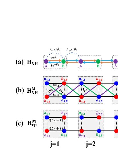
Figure 1: Schematic illustration of the non-Hermitian Kitaev chain in different representation, the dotted box indicates the unit cell. (a) The lattice structure in Dirac Fermion representation, which is described by $\mathrm{H}_{\mathrm{NH}}$. The imbalanced hopping amplitudes from A to B (orange arrow) and from B to A (blue arrow) are described by $\beta_{1}$; The imbalanced paring amplitudes of particles and holes are described by $\beta_{2}$. (b) Kitaev chain viewed as two coupled SSH chains in Majorana representation, which is described by $\mathrm{H}_{\mathrm{NH}}^{\mathrm{M}}$. The Majorana Fermion $a_{j,A/B}$ $(b_{j,A/B})$ are marked by blue (red) filled circle. The solid lines indicate the couplings $m_{1},m_{2},im_{3},im_{4}$ between nearest neighbor sites, and the dashed lines indicate the couplings $i\mu$ intra-site. (c) The lattice schematic diagram of the Hermitian counterpart systerms in Majorana representation, which is described by $\mathrm{H}_{\mathrm{cp}}^{\mathrm{M}}$.

II Non-Hermitian Kitaev chain and topological invariant

II.1 Hamiltonian of non-Hermitian Kitaev model

We introduce a 1D NH Kitaev model induced by the breakdown of chiral symmetry and particle-hole symmetry, the Hamiltonian is

$$H_{\mathrm{NH}} = -\sum_{j}[t_{L}c_{j}^{\dagger}c_{j+1}+t_{R}c_{j+1}^{\dagger}c_{j}$$ (1)

$$+\Delta^{+}c_{j}^{\dagger}c_{j+1}^{\dagger}+\Delta^{-}c_{j+1}c_{j}+\mu(1-2n_{j})],$$

where $c_{j}^{\dagger}(c_{j})$ is a fermionic creation (annihilation) operator on site $j$. As shown in Fig.1(a), we introduce the imbalanced hopping strength $\beta_{1}$ and the imbalanced SC paring strength $\beta_{2}$ in the system, which has two sublattice in a unit cell. $t_{L/R}=te^{\pm\epsilon\beta_{1}}$ denote the left/right hopping amplitude where $\epsilon=\pm 1$ for inter/intra cell. $\Delta^{\pm}=\Delta_{0}e^{\pm\beta_{2}}$ is the amplitude of $p$-wave pair creation (annihilation), $\mu$ is the chemical potential.

Then, we rewrite $H_{\mathrm{NH}}$ in the Bogoliubov-de Gennes formalism $H_{\mathrm{NH}}=C^{\dagger}h_{\mathrm{BdG}}C$ where $C$ and $C^{\dagger}$ are column and row vectors containing all canonical operators

$$C = (c_{1,A},\cdots,c_{N,B},c_{1,A}^{\dagger},\cdots,c_{N,B}^{\dagger})^{T},$$

$$C^{\dagger} = (c_{1,A}^{\dagger},\cdots,c_{N,B}^{\dagger},c_{1,A},\cdots,c_{N,B}).$$ (2)

then we can transform it to its Hermitian counterpart using a similarity transformation

$$h_{\mathrm{cp}}=S_{2}S_{1}h_{\mathrm{BdG}}S_{1}^{-1}S_{2}^{-1}$$ (3)

where the transform matrices are defined as

$$S_{1} = diag\{1,r_{1},\cdots,1,r_{1},1,r_{1}^{-1},\cdots,1,r_{1}^{-1}\},$$

$$S_{2} = diag\{r_{2},\cdots,r_{2},r_{2}^{-1},...,r_{2}^{-1}\}$$ (4)

and $r_{1}=\mathrm{exp}(-\beta_{1})$, $r_{2}=\mathrm{exp}[(\beta_{1}-\beta_{2})/2]$. So the Hamiltonian of the Hermitian counterpart read as SongZhi ; Li2018

$$H_{\mathrm{cp}}=-\sum_{j}\{(td_{j+1}^{\dagger}d_{j}+\Delta_{0}d_{j}^{\dagger}d_{j+1}^{\dagger}+h.c.)+\mu(1-2n_{j})\},$$ (5)

where the canonical operators are defined as

$$d_{j}\equiv\Omega_{j}c_{j},d_{j}^{\dagger}\equiv\Omega_{j}^{-1}c_{j}^{\dagger}$$ (6)

and the scale factors of similar transformation are

$$\Omega_{j\in odd}=e^{(\beta_{1}-\beta_{2})/2},\Omega_{j\in even}=e^{-(\beta_{1}+\beta_{2})/2}.$$ (7)

It is obvious that the operators satisfy the anti-commutation relations $\{d_{i},d_{j}^{\dagger}\}=\delta_{ij}$, $\{d_{i},d_{j}\}=\{d_{j}^{\dagger},d_{i}^{\dagger}\}=0$ and $H_{\mathrm{cp}}$ has the form of the 1D Hermitian Kitaev model.

By the Fourier transform, We can write down the Bogoliubov-de Gennes Hamiltonian in the momentum space as

$$H_{\mathrm{NH}}(k)=-\frac{1}{2}C^{{\dagger}}h(k)C$$ (8)

where $C$ and $C^{{\dagger}}$ are column and row vectors containing all canonical operators, $C=(c_{k,A},c_{k,B},c_{-k,A}^{{\dagger}}$, $c_{-k,B}^{{\dagger}})^{T},C^{{\dagger}}=(c_{k,A}^{{\dagger}},c_{k,B}^{{\dagger}},c_{-k,A},c_{-k,B})$, and the non-Hermitian matrix is

$$h(k)=\left(\begin{array}[]{cccc}-2\mu&e^{-\beta_{1}}K_{+}&0&e^{\beta_{2}}X_{+}\\ e^{\beta_{1}}K_{-}&-2\mu&-e^{\beta_{2}}X_{-}&0\\ 0&-e^{-\beta_{2}}X_{+}&2\mu&-e^{\beta_{1}}K_{+}\\ e^{-\beta_{2}}X_{-}&0&-e^{-\beta_{1}}K_{-}&2\mu\end{array}\right)$$ (9)

where $K_{\pm}=t(1+e^{\pm ik})$, $X_{\pm}=\Delta_{0}(1-e^{\pm ik})$. Diagonalizing $h(k)$, we can get the energy dispersion

$$E(k)=\pm 2\sqrt{(t\cos(k)-\mu)^{2}+\Delta^{2}\sin^{2}(k)},$$ (10)

which can’t be affected by the non-Hermitian parameter $\beta_{1},\beta_{2}$ and is just the spectrum of $\beta_{1}=\beta_{2}=0$. It should be noticed that there is no skin effect for the system Yao2018 ; YaoWang2018 ; SongWang2019 ; Deng2019 ; Longhi2019 . Therefore, one can calculate the gap closing point $E(k)=0$ to get the topological phase boundary of the system. As a result, the Majorana edge modes emerge in the topological phase $|\mu/t|<1$.

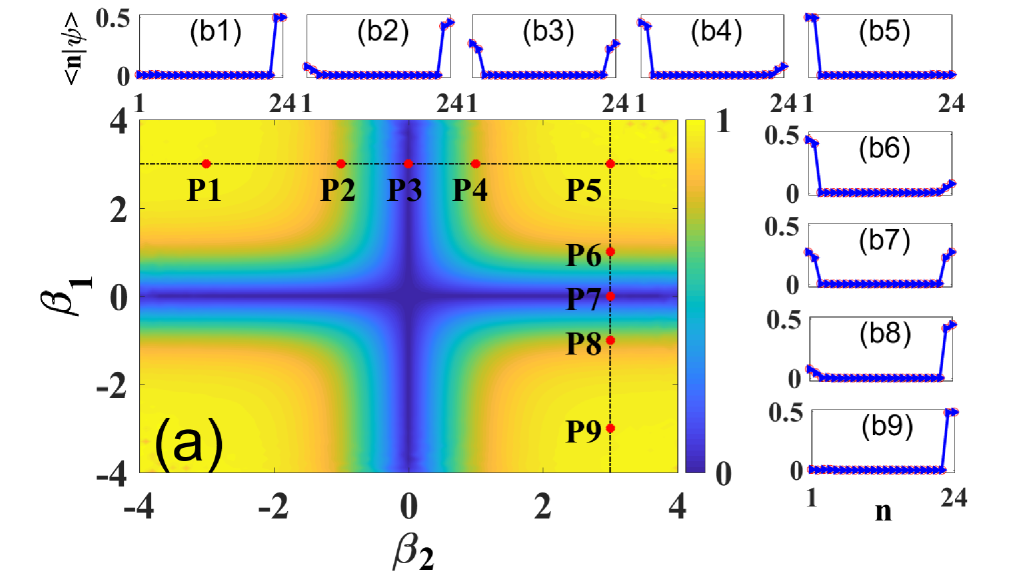
Figure 2: Similarity $\gamma_{\mathrm{M}}$ and localized properties of the two defective MZMs with $L=24$, $\mu=0.1$, $t=1$ and $\Delta_{0}=0.8$. (a) The blue area represent $\gamma_{\mathrm{M}}=0$ which means two MZMs local at two end of the chain independently, the yellow areas represent $\gamma_{\mathrm{M}}=1$ which means the two MZMs coalesce to one and local at either left or right end of the chain. (b1-b9) The distributions of the MZMs for different cases marked by the points P1-P9 in (a), respectively. For the cases in P1, P5, P9, which are away from $\beta_{1}=0$ and $\beta_{2}=0$, the two MZMs coalesce to one.

II.2 Biorthogonal $\mathrm{Z}_{2}$ topological invariant

Then, we investigate the topological properties of the NH Kitaev chain $H_{\mathrm{NH}}$. The fermion Hamiltonian in momentum space is divided into three parts,

$$\mathrm{\hat{H}}_{\mathrm{NH}}=\mathrm{\hat{H}}_{\mathrm{NH},k>0}+\mathrm{\hat{H}}_{\mathrm{NH},k=0}+\mathrm{\hat{H}}_{\mathrm{NH},k=\pi}.$$ (11)

After diagonalizing the fermion Hamiltonian at the points $k>0$, we have

$$\mathrm{\hat{H}}_{\mathrm{NH},k>0}=\sum_{k\mathbf{>}0}\varepsilon(k)\alpha_{k}^{{\dagger}}\alpha_{k}-\sum_{k>0}\varepsilon(k)\alpha_{-k}\alpha_{-k}^{\dagger}$$ (12)

where $\alpha_{k}$ are diagonalized quasi-particles operators and $\alpha_{\pm k}$ annihilate the ground state $|G\rangle$, i.e., $\alpha_{\pm k}|G\rangle=0$. Both $\alpha$ band has a positive energy at each point in momentum space $k>0$. The Hamiltonian at $k=0$ and $k=\pi$ are diagonalized into

$$\mathrm{\hat{H}}_{\mathrm{NH},k=0} =\varepsilon(k=0)\alpha_{k=0}^{{\dagger}}\alpha_{k=0},$$

$$\mathrm{\hat{H}}_{\mathrm{NH},k=\pi} =\varepsilon(k=\pi)\alpha_{k=\pi}^{{\dagger}}\alpha_{k=\pi}$$ (13)

where $\varepsilon(k=0)=\mu-t$ and $\varepsilon(k=\pi)=\mu+t.$

Based on the biorthogonal set, the right/left eigenstates and corresponding eigenvalues for the NH systems satisfy the relationship $\mathrm{\hat{H}}_{\mathrm{NH}}|{\Psi}_{m}^{\mathrm{R}}\rangle=E_{m}|{\Psi}_{m}^{\mathrm{R}}\rangle,$ and $\mathrm{\hat{H}}_{\mathrm{NH}}^{\dagger}|{\Psi}_{m}^{\mathrm{L}}\rangle=E_{m}^{\ast}|{\Psi}_{m}^{\mathrm{L}}\rangle$. To describe this topological structure of $\mathrm{\hat{H}}_{\mathrm{NH}}$, we define biorthogonal $Z_{2}$ topological invariant,

$$\mathcal{\omega}=\mathrm{sgn}(\eta_{{}_{k=0}}\cdot\eta_{{}_{k=\pi}})$$ (14)

where

$$\eta_{{}_{k=0}} =\left\langle{\Psi}_{0}^{\mathrm{L}}\right|c_{k=0}^{\dagger}c_{k=0}\left|{\Psi}_{0}^{\mathrm{R}}\right\rangle{},$$

$$\eta_{{}_{k=\pi}} =\left\langle{\Psi}_{0}^{\mathrm{L}}\right|c_{k=\pi}^{\dagger}c_{k=\pi}\left|{\Psi}_{0}^{\mathrm{R}}\right\rangle.$$ (15)

Here, $\left|{\Psi}_{0}^{\mathrm{R}}\right\rangle$ denotes the ground state, $\Delta_{0}=t$, and

$$\eta_{{}_{k\mathbf{=}0}} =\frac{\varepsilon[k=0\mathbf{]}}{\left|\varepsilon[k=0\mathbf{)]}\right|}=\frac{\mu-t}{\left|\mu-t\right|},$$

$$\eta_{{}_{k\mathbf{=}\pi}} =\frac{\varepsilon[k=\pi\mathbf{]}}{\left|\varepsilon[k=\pi\mathbf{)]}\right|}=\frac{t+\mu}{\left|t+\mu\right|}.$$ (16)

As a results, we have

$$\eta_{{}_{k=0}} =\{\begin{array}[c]{l}+1,\text{ }\varepsilon\left(k=0\right)>0\\ -1,\text{ }\varepsilon\left(k=0\right)<0\end{array},$$ (19)

$$\eta_{{}_{k=\pi}} =\{\begin{array}[c]{l}+1,\text{ }\varepsilon\left(k=\pi\right)>0\\ -1,\text{ }\varepsilon\left(k=\pi\right)<0\end{array}.$$ (22)

Then $\mathcal{\omega}$ becomes topological invariant to characterize the universal properties of different topological phases, $\mathcal{\omega}=1$ with $(\eta_{k=0},\eta_{k=\pi})=\left(-1,-1\right)$ or $\left(1,1\right)$ represent two trivial SCs, and $\mathcal{\omega}=-1$ with $(\eta_{k=0},\eta_{k=\pi})=\left(-1,1\right)$ or $\left(1,-1\right)$ represent two topological SCs, where there exist two MZMs located at two end of the 1D Kitaev chain.

III Defective Majorana edge states

III.1 Hamiltonian in Majorana representation

By introduce Majorana Fermion $a_{n}=c_{n}^{{\dagger}}+c_{n}$, $b_{n}=-i(c_{n}^{{\dagger}}-c_{n})$, the non-Hermitian Hamiltonian $H_{\mathrm{NH}}$ can be written in Majorana-representation:

$$H^{\mathrm{M}}_{\mathrm{NH}}= - \frac{1}{4}\sum_{j}[m_{1}(a_{j,A}a_{j,B}-b_{j,B}b_{j+1,A})$$ (23)

$$+ m_{2}(b_{j,A}b_{j,B}-a_{j,B}a_{j+1,A})$$

$$+ im_{3}(b_{j,A}a_{j,B}+b_{j,B}a_{j+1,A})$$

$$+ im_{4}(-a_{j,A}b_{j,B}-a_{j,B}b_{j+1,A})$$

$$+ i4\mu(a_{j,A}b_{j,A}+a_{j,B}b_{j,B})],$$

where the coupling $m_{1},m_{2},im_{3},im_{4}$ between nearest neighbor sites are:

$$m_{1} = t\sinh(\beta_{1})+\Delta_{0}\sinh(\beta_{2}),$$

$$m_{2} = t\sinh(\beta_{1})-\Delta_{0}\sinh(\beta_{2}),$$

$$m_{3} = t\cosh(\beta_{1})+\Delta_{0}\cosh(\beta_{2}),$$

$$m_{4} = -t\cosh(\beta_{1})+\Delta_{0}\cosh(\beta_{2}).$$ (24)

As shown in Fig.1(b), the system contains four Majorana Fermions in each unit cell. the Majorana Fermion $a_{j,A/B}$ $(b_{j,A/B})$ are marked by blue (red) filled circle, the solid lines indicate the couplings $m_{1},m_{2},im_{3},im_{4}$ between nearest neighbor sites, and the dashed lines indicate the couplings $i\mu$ intra-site.

III.2 Analytic results of the defective MZMs

To acquire the correspondence of topological number $\mathcal{Z}$ and the number of edge stats for the finite size chain $\mathcal{C}_{\mathrm{finite}}$, we can investigate the analytic expression of edge states under the open boundary condition. We begin from the zero-mode eigenstates in the semi-infinite limit from the right or left boundary.

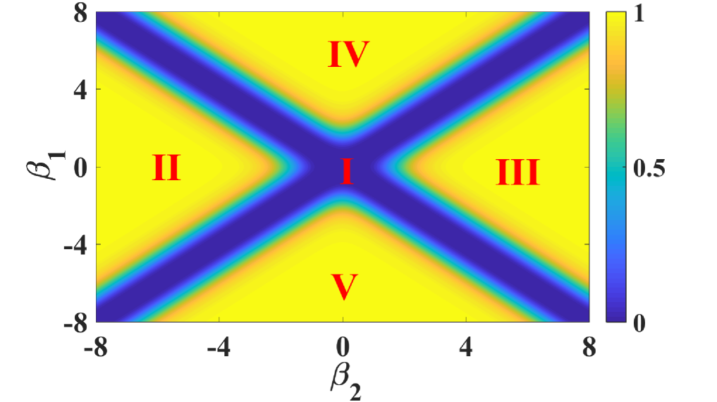
Figure 3: Similarity $\gamma_{\mathrm{spin}}$ of the two ground states in spin-representation with $L=4$, $t=\Delta_{0}=1$ and $\mu=0.1$. The blue area I represents $\gamma_{\mathrm{spin}}=0$ which means the two ground states are orthogonal, The yellow area II-V represent $\gamma_{\mathrm{spin}}=1$ which means the two ground states coalesce to one and act as exceptional points (EPs).

In order to avoid confusion with the operators $c_{j},c_{j}^{\dagger}$ in $H_{\mathrm{NH}}$, we rewrite it’s Hermitian counterpart $H_{\mathrm{cp}}$ in Eq.(5) by substituting the notation simply: $\{d_{j},d_{k}^{\dagger}\}\rightarrow\{\bar{c}_{j},\bar{c}_{k}^{\dagger}\}$, i.e., $H_{\mathrm{cp}}=\bar{C}^{\dagger}h_{\mathrm{cp}}\bar{C}$, which is written as

$$H_{\mathrm{cp}}=-\sum_{j}\{(t\bar{c}_{j+1}^{\dagger}\bar{c}_{j}+\Delta_{0}\bar{c}_{j}^{\dagger}\bar{c}_{j+1}^{\dagger}+h.c.)-\mu(1-2\bar{n}_{j})\},$$ (25)

this is just the 1D Hermitian Kitaev model. Therefore, we can investigate the non-Hermitian properties of $H_{\mathrm{NH}}$ based on its Hermitian counterpart $H_{\mathrm{cp}}$, with the definition of Majorana operators

$$\bar{c}_{j}^{\dagger}=\frac{1}{2}(\bar{a}_{j}+i\bar{b}_{j}),\bar{c}_{j}=\frac{1}{2}(\bar{a}_{j}-i\bar{b}_{j})$$ (26)

we rewrite the Hamiltonian $H_{\mathrm{cp}}$ by Majorana operators,

$$H_{\mathrm{cp}}^{\mathrm{M}}=\frac{-i}{2}\sum_{j=1}^{L}\{(t-\Delta_{0})\bar{b}_{j+1}\bar{a}_{j}+(t+\Delta_{0})\bar{b}_{j}\bar{a}_{j+1}+2\mu\bar{a}_{j}\bar{b}_{j}\}$$ (27)

The lattice schematic diagram of $H_{\mathrm{cp}}^{\mathrm{M}}$ is shown in Fig.1(c). As we know, in the Hermitian cases, two unpaired Majorana zero mode would locate at the right and left end of the Kitaev chain. Besides, for a finite size chain with $\mu\neq 0$, the eigne energy of the two Majorana edge modes can split due to the coupling of them.

Next, we try to acquire the analytic expression for the edge states. Firstly, we consider a very long wire, which means the Majorana edges modes have zero energy; We calculate their wave functions by using the Heisenberg equations of motion

$$[H_{\mathrm{cp}}^{\mathrm{M}},\bar{a}_{m}]=0,[H_{\mathrm{cp}}^{\mathrm{M}},\bar{b}_{m}]=0,$$ (28)

where $\bar{a}_{m}$, $\bar{b}_{m}$ are the two Majorana operators at site n which were denoted by $\bar{a}_{n,A},\bar{a}_{n,B}$ and $\bar{b}_{n,A},\bar{b}_{n,B}$ above. We obtain the difference equations for these operators as SemiFinit ; SemiFinit2 :

$$(t+\Delta_{0})\bar{b}_{m}+(t-\Delta_{0})\bar{b}_{m+1}+2\mu\bar{b}_{m} = 0$$

$$(t-\Delta_{0})\bar{a}_{m}+(t+\Delta_{0})\bar{a}_{m+1}+2\mu\bar{a}_{m} = 0$$ (29)

for $2\leq m\leq 2L-1$, These difference equations can be solved exactly by using $Z$-transform methods. We introducing a power series

$$A(z)=\sum_{m=0}^{\infty}z^{-m}\bar{a}_{m}\equiv Z[\bar{a}_{m}]$$ (30)

where $z$ is a complex variable. The function $A(z)=Z[\bar{a}_{m}]$ is called the $Z$-transform of $\bar{a}_{m}$. Taking the $Z$-transform of the above difference equation and using properties such

$$Z[\bar{a}_{m-1}]=z^{-1}A(z),Z[\bar{a}_{m+1}]=zA(z)-z\bar{a}_{0}$$ (31)

$\bar{a}_{0}$ is a constant determined by boundary conditions, one can obtain a closed form expression for the $Z$-transform $A(z)$, given by:

$$A(z)=\frac{\bar{a}_{0}z^{2}}{z^{2}+\frac{\mu}{t-\Delta_{0}}z+\frac{t+\Delta_{0}}{t-\Delta_{0}}}$$ (32)

This $Z$-transform has a unique inverse, which is the exact solution to the difference equation. Thus the obtained wave function is

$$\bar{a}_{m} = \bar{a}_{0}C^{m}\left[\cos(\theta m)+\frac{1}{\tan\theta}\sin(\theta m)\right]$$ (33a)

$$\bar{b}_{m} = \bar{b}_{0}C^{-m}\left[\cos(\theta m)+\frac{1}{\tan\theta}\sin(\theta m)\right]$$ (33b)

where

$$C=\sqrt{\frac{t-\Delta_{0}}{t+\Delta_{0}}},\theta=\arctan\frac{\sqrt{t^{2}-\Delta_{0}^{2}-\mu^{2}}}{\mu}$$ (34)

The entire model is equivalent to two coupled SSH like chains containing both the hopping parameters $i(\Delta_{0}-t)$ and $i(\Delta_{0}+t)$, as shown in Fig.1(c). Here, we only concentrate on the zero energy eigne states, the excited states in complex and is not important here. If $t>\Delta_{0}>0,\mu\neq 0$, the system has two gap states, one can get the analytical wave function of the zero energy mode (gap states) in Majorana-representation. Here we express the zero mode of $H_{\mathrm{cp}}^{\mathrm{M}}$ in $\bar{a}$-sublattice and $\bar{b}$-sublattice as (i.e. the states in the left and right edges)

$$\left|\psi\right\rangle_{a}^{L} = \sum_{m=0}^{L-1}\Lambda(m)\left|m\right\rangle\otimes\left(\begin{array}[]{c}\bar{a}\\ 0\end{array}\right)$$ (37)

$$\left|\psi\right\rangle_{b}^{R} = \sum_{m=0}^{L-1}\Lambda(m)\left|L-m\right\rangle\otimes\left(\begin{array}[]{c}0\\ \bar{b}\end{array}\right)$$ (40)

where we set $\bar{a}_{0,A}=\bar{b}_{N,B}=1$, $\Lambda(m)=C^{m}\Theta(m)$

$$\Theta(m)=\left[\cos(\theta m)+\frac{1}{\tan\theta}\sin(\theta m)\right].$$ (41)

When the region we considerate is $\mu^{2}<4(t^{2}-\Delta_{0}^{2})$ predict an oscillatory exponential decay of the coefficients: $e^{-n/2\zeta}$ for $\left|\psi\right\rangle_{\bar{a}}$, where the decay length $\zeta$ is defined by

$$\zeta=1/\left|\ln\left(\frac{t-\Delta_{0}}{t+\Delta_{0}}\right)\right|$$ (42)

So with the inverse similarity transformation based on Eq. (6), Eq. (25) and Eq. (26), we exchange the operator by the rule $(\bar{a}_{j},\bar{b}_{j})\rightarrow(\bar{c}_{j}^{\dagger},\bar{c}_{j})\rightarrow(d_{j}^{\dagger},d_{j})\rightarrow(c_{j}^{\dagger},c_{j})$, and we get the anti-zero-energy modes (edge states) for the initial non-Hermitian Hamiltonian $H_{\mathrm{NH}}$ in Nambu representation, as shown in Eq.(2). The right-vectors of the right/left localized edge states are expressed as

$$\left|\psi_{\mathrm{NH}}^{\mathrm{R}}\right\rangle = \frac{i}{\sqrt{\mathcal{N}_{b}}}\sum_{m=1}^{L}\Lambda(L-m+1)[\Omega_{m}^{-1}\left|m\right\rangle-\Omega_{m}\left|L+m\right\rangle],$$

$$\left|\psi_{\mathrm{NH}}^{\mathrm{L}}\right\rangle = \frac{1}{\sqrt{\mathcal{N}_{a}}}\sum_{m=1}^{L}\Lambda(m)[\Omega_{m}^{-1}\left|m\right\rangle+\Omega_{m}\left|L+m\right\rangle],$$ (43)

where $L=2N$ is the length of the Majorana ladder, $\Omega_{\mathrm{m\in odd}}=e^{(\beta_{1}-\beta_{2})/2}$, $\Omega_{\mathrm{m\in even}}=e^{-(\beta_{1}+\beta_{2})/2}$.

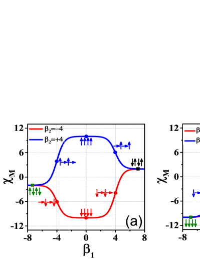
Figure 4: The spin structure of the many-body ground state $\left|G\right\rangle_{\mathrm{NH}}^{1}$ with (a) $\beta_{2}=\pm 4$ and (b) $\beta_{1}=\pm 4$. Here, we set $L=4$, $t=\Delta_{0}=1$ and $\mu=0.1$. The non-Hermitian suppression effect, induced by the competition of $\beta_{1}$ and $\beta_{2}$, drives the spin flipping to opposite direction continuously without gap closing.

Similarly, we can get the left-vector $\left\langle\Phi\right|$ of the zero mode edge states defined by $\left\langle\Phi\right|H=\left\langle\Phi\right|E$ , or $H^{\dagger}\left|\Phi\right\rangle=E^{\ast}\left|\Phi\right\rangle$. We can use the exchange $te^{-\beta_{1}}\leftrightarrow te^{\beta_{1}}$, $\Delta_{0}e^{\beta_{2}}\leftrightarrow\Delta_{0}e^{-\beta_{2}}$, $\Omega\leftrightarrow\Omega^{-1},$ for convenience, the left-vector for the right/left localized edges states can be expressed as

$$\left|\Phi_{\mathrm{NH}}^{\mathrm{R}}\right\rangle = \frac{i}{\sqrt{\mathcal{N}_{b}}}\sum_{m=1}^{L}\Lambda(L-m+1)[\Omega_{m}\left|m\right\rangle-\Omega_{m}^{-1}\left|L+m\right\rangle],$$

$$\left|\Phi_{\mathrm{NH}}^{\mathrm{L}}\right\rangle = \frac{1}{\sqrt{\mathcal{N}_{a}}}\sum_{m=1}^{L}\Lambda(m)[\Omega_{m}\left|m\right\rangle+\Omega_{m}^{-1}\left|L+m\right\rangle],$$ (44)

where $\mathcal{N}_{a}=\mathcal{N}_{b}=\sum_{m=1}^{L}2\Lambda(m)^{2}\equiv\mathcal{N}$ is biorthogonal normalization coefficient.

Next, taking $(\left|\psi_{\mathrm{NH}}^{\mathrm{R}}\right\rangle,\left|\psi_{\mathrm{NH}}^{\mathrm{R}}\right\rangle)$ and $(\left\langle\Phi_{\mathrm{NH}}^{\mathrm{L}}\right|,\left\langle\Phi_{\mathrm{NH}}^{\mathrm{R}}\right|)$ as the basis states, we construct the effective Hamiltonian of edge states for the finite-size Kitaev chain as

$$\mathcal{H}_{\mathrm{edge}}=\left(\begin{array}[]{cc}h_{\mathrm{LL}}&h_{\mathrm{LR}}\\ h_{\mathrm{RL}}&h_{\mathrm{RR}}\end{array}\right),$$ (47)

where the elements of $\mathcal{H}_{\mathrm{edge}}$ are defined as $h_{\mathrm{I,J}}=\left\langle\Phi^{\mathrm{I}}_{\mathrm{NH}}|H_{\mathrm{NH}}|\psi^{\mathrm{J}}_{\mathrm{NH}}\right\rangle$ and $\mathrm{I,J=L,R}$. We have $h_{\mathrm{LL}}=h_{\mathrm{RR}}=0,h_{\mathrm{RL}}=h_{\mathrm{LR}}^{\ast}=i\xi$, i.e.,

$$\mathcal{H}_{\mathrm{edge}}=\left(\begin{array}[]{cc}0&-i\xi\\ i\xi&0\end{array}\right)=\xi\sigma_{y}$$ (50)

where $\sigma_{y}$ denotes the Pauli matrices acting on the subspace of two edge states and $\xi$ is the coupling coefficient of them SemiFinit3 :

$$\xi = \frac{\sqrt{t^{2}-\Delta_{0}^{2}}^{L+1}}{4\sin^{3}\theta}\{2\sin(\theta L)$$ (51)

$$+ L\sin[\left(L+2\right)\theta]-L\sin\left[\left(L+4\right)\theta\right]\}$$

The energy of MZMs are $E_{\mathrm{edge}}^{\pm}=\pm\sqrt{|\xi|}$ and in the thermodynamic limit ($L\mapsto+\infty$) we have $E^{\pm}_{\mathrm{edge}}\mapsto 0$. Because the eigenstates of $\sigma_{y}$ is $(1,i)$ and $(1,-i)$, the eigenstates of $\mathcal{H}_{\mathrm{edge}}$ (i.e. the eigen wavefunction of edge states) are

$$\left|\psi^{+}\right\rangle = \frac{1}{\sqrt{2\mathcal{N}}}\left(\left|\psi_{\mathrm{NH}}^{\mathrm{L}}\right\rangle+i\left|\psi_{\mathrm{NH}}^{\mathrm{R}}\right\rangle\right),$$

$$\left|\psi^{-}\right\rangle = \frac{1}{\sqrt{2\mathcal{N}}}\left(\left|\psi_{\mathrm{NH}}^{\mathrm{L}}\right\rangle-i\left|\psi_{\mathrm{NH}}^{\mathrm{R}}\right\rangle\right).$$ (52)

So far, we get the analytic solution of the non-Hermitian Majorana zero modes.

III.3 Number-anomalous bulk-boundary correspondence

Then, to describe the localization and the orthogonality of the two edge states, i.e., to investigate the bulk-boundary correspondence of the NH system, we define the similarity of the two edge states as

$$\gamma_{\mathrm{M}}\equiv\left\langle\psi^{-}|\psi^{+}\right\rangle=\left(e^{-\beta_{1}}-e^{\beta_{1}}\right)\left(e^{\beta_{2}}-e^{-\beta_{2}}\right)\kappa,$$ (53)

where $\kappa=\frac{1}{2\mathcal{N}}\sum_{n=0}^{L-1}(-1)^{n}C^{2n}\Theta_{n}^{2}$ is a nonzero value independent of $\beta_{1}$ and $\beta_{2}$. When $\beta_{1,2}\neq 0$ we have $\gamma_{\mathrm{M}}\neq 0$, which means the two edge states $\left|\psi^{\pm}\right\rangle$ are not orthogonal and no longer located at two ends of the chain respectively. The distributions of similarity $\gamma_{\mathrm{M}}(\beta_{1},\beta_{2})$ and corresponding eigen wavefunction are calculated numerically and are shown in Fig.2. We can see that, $\gamma_{\mathrm{M}}$ tends to be 1 when the NH strength $\beta_{1}$ and $\beta_{2}$ are away from 0, this means the two MZMs become one gradually and evolve to the exceptional points (EPs) eventually. As a result, the typical BBC is broken and the MZM local only at the left or right end of the system. For example, when $\beta_{1}=\beta_{2}=3$ (point P5 in Fig.2(a)), $\gamma_{\mathrm{M}}=1$ and the Majorana zero mode only locate at left end of the chain (shown in (b5) of Fig.2(b)).

Therefore, the number-anomalous BBC can be defined as kou2020

$$\mathcal{C}_{\mathrm{finite}}=2-\gamma_{\mathrm{M}}.$$ (54)

In the Hermitian case ($\beta_{1}=\beta_{2}=0$), we have $\gamma_{\mathrm{M}}=0$, the number of MZMs is $\mathcal{C}_{\mathrm{finite}}=2$ and the typical BBC is acquired. While, in the NH cases ($\beta_{1,2}\neq 0$), we have $0<\gamma_{\mathrm{M}}\leq 1$, the MZMs becomes defective and we have $1\leq\mathcal{C}_{\mathrm{finite}}\leq 2$. A special case is $\mathcal{C}_{\mathrm{finite}}=1$, which indicates the existence of a singular MZM. This phenomenon didn’t occur in previous studies, neither in Hermitian nor in NH SC systems.

There are two reasons for this observation: the breakdown of sublattice symmetry induced by $\beta_{1}$ and the breakdown of the particle-hole symmetry induced by $\beta_{2}$. As shown in the Fig.1(a), the imbalanced particle hopping lead to the breakdown of sublattice symmetry, which can suppress the particles located at A-sublattice ($\beta_{1}<0$) or B-sublattice ($\beta_{1}>0$). Meanwhile, the imbalanced paring amplitudes lead to the breakdown of the particle-hole symmetry, which make the Majorana quasi-particle behave particle-like or hole-like. In a word, the defective Majorana zero modes are induced by the breakdown of sublattice symmetry and particle-hole symmetry.

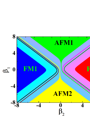
Figure 5: Global magnetic phase diagram of the many-body ground states. The variations of $\chi_{\mathrm{M}}$ induced by non-Hermitian suppression effect are marked by different colors: FM phase (blue and red area), AFM phase (green and yellow area) and so on. Here, we set $L=4$, $t=\Delta_{0}=1$ and $\mu=0.1$.

IV Many-body correspondence of the defective MZMs

Benefit from the mapping between Kitaev chain and spin chain, one can simulate the MZMs in the Ising language via a Jordan-Wigner transformation JWTran1 ; JWTran2 , because the Ising model is relatively easy to implement. For example, MZMs have attracted much attention due to their potential application in topological quantum computations, the spin chain can be used to simulate the braiding of these MZMs, which corresponding to the topological quantum gates Guo2016 . Therefore, it is necessary to explore the many-body correspondence of the defective MZMs and explain the NH effects on the spin-representation.

	$\ \ \ \left|G\right\rangle_{\mathrm{NH}}^{1}\ \ \$	$\ \ \ \left|G\right\rangle_{\mathrm{NH}}^{2}\ \ \$	$\ \ \ \ \ \ \ \ \chi_{\mathrm{M}}\ \ \ \ \ \ \ \ \$	$\gamma_{\mathrm{spin}}$	Phase
$\beta_{1}=0,\beta_{2}\rightarrow+\infty$	$\left|\uparrow\uparrow\uparrow\uparrow\right\rangle$	$\left|\uparrow\uparrow\uparrow\uparrow\right\rangle$	$L(L+1)/2$	$1$	FM2
$\beta_{1}=0,\beta_{2}\rightarrow-\infty$	$\left|\downarrow\downarrow\downarrow\downarrow\right\rangle$	$\left|\downarrow\downarrow\downarrow\downarrow\right\rangle$	$-L(L+1)/2$	$1$	FM1
$\beta_{2}=0,\beta_{1}\rightarrow+\infty$	$\left|\downarrow\uparrow\downarrow\uparrow\right\rangle$	$\left|\downarrow\uparrow\downarrow\uparrow\right\rangle$	$L/2$	$1$	AFM1
$\beta_{2}=0,\beta_{1}\rightarrow-\infty$	$\left|\uparrow\downarrow\uparrow\downarrow\right\rangle$	$\left|\uparrow\downarrow\uparrow\downarrow\right\rangle$	$-L/2$	$1$	AFM2
$\beta_{1}=\beta_{2}>0$	$\left|\rightarrow\uparrow\rightarrow\uparrow\right\rangle$	$\left|\leftarrow\uparrow\leftarrow\uparrow\right\rangle$	$L(L+2)/4$	$0$	Even-FM2
$\beta_{1}=\beta_{2}<0$	$\left|\rightarrow\downarrow\rightarrow\downarrow\right\rangle$	$\left|\leftarrow\downarrow\leftarrow\downarrow\right\rangle$	$-L(L+2)/4$	$0$	Even-FM1
$\beta_{1}=-\beta_{2}<0$	$\left|\uparrow\rightarrow\uparrow\rightarrow\right\rangle$	$\left|\uparrow\leftarrow\uparrow\leftarrow\right\rangle$	$L^{2}/4$	$0$	Odd-FM2
$\beta_{1}=-\beta_{2}>0$	$\left|\downarrow\rightarrow\downarrow\rightarrow\right\rangle$	$\left|\downarrow\leftarrow\downarrow\leftarrow\right\rangle$	$-L^{2}/4$	$0$	Odd-FM1

Table 1: The non-Hermitian effects on the two ground states in different limit cases (first collum). The spin configurations, magnetic factor $\chi_{\mathrm{M}}$, similarity rate $\gamma_{\mathrm{spin}}$ and magnetic phase are shown in collum 2-6, respectively.

IV.1 NH spin model corresponding to the NH Kitaev model

In the Hermitian case, it has been noted that the Kitaev model can be mapped to the Ising model via the Jordan-Wigner transformation, and the two MZMs can also be mapped to the two degenerate ground states of the Ising model. Similarly, we can transform the NH Kitaev model to NH Ising model in this way. The Hamiltonian $H_{\mathrm{NH}}$ can be written in spin-representation as

$$H_{\mathrm{NH}}^{\mathrm{spin}} = -\frac{1}{4}\sum_{j}\{J_{1}\sigma_{j}^{x}\sigma_{j+1}^{x}+J_{2}\sigma_{j}^{y}\sigma_{j+1}^{y}$$ (55)

$$+iJ_{3}\sigma_{j}^{x}\sigma_{j+1}^{y}+iJ_{4}\sigma_{j}^{y}\sigma_{j+1}^{x}+4\mu\sigma_{j}^{z}\},$$

where

$$J_{1} = t\cosh\beta_{1}+\Delta_{0}\cosh\beta_{2},$$

$$J_{2} = t\cosh\beta_{1}-\Delta_{0}\cosh\beta_{2},$$

$$J_{3} = \epsilon t\sinh\beta_{1}+\Delta_{0}\sinh\beta_{2},$$

$$J_{4} = -\epsilon t\sinh\beta_{1}+\Delta_{0}\sinh\beta_{2}.$$ (56)

And $H_{\mathrm{NH}}^{\mathrm{spin}}$ can also be transformed to a Hermitian Hamiltonian by the similarity transformation

$$H_{\mathrm{cp}}^{\mathrm{spin}}=UH_{\mathrm{NH}}^{\mathrm{spin}}U^{-1},$$ (57)

where the similarity transformation operator can be expressed as $U={\prod}_{j}\otimes U_{j,A}\otimes U_{j,B},$ where

$$U_{j,A}=diag\{1,\mathrm{exp}[(\beta_{2}-\beta_{1})/2]\},$$

$$U_{j,B}=diag\{1,\mathrm{exp}[(\beta_{2}+\beta_{1})/2]\}.$$ (58)

Therefore, the Hermitian counterpart of $H_{\mathrm{NH}}$ in spin-representation can be expressed as

$$H_{\mathrm{cp}}^{\mathrm{spin}}=-\sum_{j=1}^{L-1}\{J_{x}\sigma_{j}^{x}\sigma_{j+1}^{x}+J_{y}\sigma_{j}^{y}\sigma_{j+1}^{y}-2\mu\sigma_{j}^{z}\},$$ (59)

where $J_{x/y}=t\pm\Delta_{0}$ and this is just the quantum XY spin chain and its extensions have been studied from many different perspectives.

IV.2 Similarity of the two degenerate ground states

To characterize the properties of ground states, we calculate the magnetic factor when the system is in its ground state. Firstly, for simplicity and typicality, we consider the limit case $\mu=0$, $t=\Delta_{0}$ where $H_{\mathrm{cp}}^{\mathrm{spin}}$ is exactly the Ising model without transverse field, the ground states of $H_{\mathrm{cp}}^{\mathrm{spin}}$ are described as

$$\left|G\right\rangle_{\mathrm{cp}}^{1}=\left|\rightarrow\rightarrow\cdots\rightarrow\right\rangle,\left|G\right\rangle_{\mathrm{cp}}^{2}=\left|\leftarrow\leftarrow\cdots\leftarrow\right\rangle.$$ (60)

So the ground states of initial NH spin chain can be obtained completely under the inverse similarity transformation:

$$\left|G\right\rangle_{\mathrm{NH}}^{1}=U^{-1}\left|G\right\rangle_{\mathrm{cp}}^{1},\left|G\right\rangle_{\mathrm{NH}}^{2}=U^{-1}\left|G\right\rangle_{\mathrm{cp}}^{2}.$$ (61)

In fact, $U_{i}$ act as a transverse field inner each site $i$. When we adjust $\beta_{1}$ and $\beta_{2}$, the two ground states may construct different spin structure in the spin chain. Then, we define the similarity of the two ground states as

$$\gamma_{\mathrm{spin}}(\beta_{1},\beta_{2})={}_{\mathrm{NH}}^{~{}~{}~{}2}\left\langle G|G\right\rangle^{1}_{\mathrm{NH}},$$ (62)

After a tedious calculation, we can obtain

$$\gamma_{\mathrm{spin}}(\beta_{1},\beta_{2})=(-\tanh[\frac{(\beta_{1}+\beta_{2})}{2}]\tanh[\frac{(\beta_{1}-\beta_{2})}{2}])^{\frac{L}{2}}$$ (63)

Therefore, $\gamma_{\mathrm{spin}}$ will change with $\beta_{1}$ and $\beta_{2}$. It is obvious that $\left|G\right\rangle_{\mathrm{NH}}^{1}$ and $\left|G\right\rangle_{\mathrm{NH}}^{2}$ are not always orthogonal. We study this phenomena in some limiting case: (1) when $\beta_{1}=0$, we have $\gamma_{\mathrm{spin}}(0,\beta_{2})=[\tanh(\frac{\beta_{2}}{2})]^{L}$; (2) When $\beta_{2}=0$, we have $\gamma_{\mathrm{spin}}(\beta_{1},0)=[-\tanh(\frac{\beta_{1}}{2})]^{L}$; (3) when $\beta_{1}=\beta_{2}$, we have $\gamma_{\mathrm{spin}}(\beta_{1}=\beta_{2})=0$. Indeed, for spin systems with finite size, two ground states will coalesce when $\beta_{1}\mapsto 0$(or $\beta_{2}\mapsto 0$). While, two ground states can’t coalesce in the thermodynamic limit $L\mapsto\infty$, due to $\tanh(\beta_{1/2})<1$.

Now, we take 4-spin systems as an example and show the coalescence phase diagram in Fig.(3). We can see that $\gamma_{\mathrm{spin}}\mapsto 0$ when the NH strengths are near $\beta_{1}=\beta_{2}$ region, and $\gamma_{\mathrm{spin}}\mapsto 1$ when $\beta_{1},\beta_{2}$ are large enough which means the wave functions of the two degenerate ground states coalesce. This is very different from the similarity of MZM in Majorana representation shown in Fig.(2), where $\gamma_{\mathrm{M}}\rightarrow 0$ in the region near $\beta_{1}=0$, or $\beta_{2}=0$.

IV.3 Phase crossover without gap closing

An important question is why the coalescing phase diagram of MZMs shown in Fig.(2) is totally different from the coalescing phase diagram of spin ground states shown in Fig.(3), i.e.

$$\gamma_{\mathrm{M}}(\beta_{1},\beta_{2})\neq\gamma_{\mathrm{spin}}(\beta_{1},\beta_{2}).$$ (64)

The key point is the correspondence of single-particle and the many-body systems. We know that the relation of MZMs and the ground states of spin system is

$$\left|G\right\rangle_{\mathrm{NH}}^{1/2}=\hat{\psi}^{\mathrm{L/R}}_{\mathrm{NH}}\left|F\right\rangle,$$ (65)

where $\left|F\right\rangle$ is the many-body vacuum state in spin-representation, and it is also the many-body quantum state with occupied single particle states for $E<0$ and empty single particle states for $E\geq 0$. Therefore, the single-body wave function $\left|\psi^{\mathrm{L/R}}_{\mathrm{NH}}\right\rangle$ shown in Eq.43 can’t describe the many-body ground states absolutely, we must take $\left|F\right\rangle$ into account. Indeed, the NH terms perturb the vacuum background also, even they do not change the energy of the states.

To give a quantitative description for the spin configurations of the two ground states in the spin system, we define a magnetic factor as

$$\chi_{\mathrm{M}}(\beta_{1},\beta_{2})\equiv\sum_{n=1}^{L}{~{}}_{\mathrm{NH}}^{~{}~{}~{}1}\left\langle G\right|\negmedspace n\sigma_{n}^{z}\left|G\right\rangle_{\mathrm{NH}}^{1},$$ (66)

where a weighted sum of the spin of the n-th lattice is introduced. The introduce of the lattice number ”n” can distinguish each site, so the magnetic factor $\chi_{\mathrm{M}}(\beta_{1},\beta_{2})$ contains all spin information in each site. Then, we take the lattice size $L=4$ as an example, and give the magnetic susceptibility and spin configurations of the many-body ground states $\left|G\right\rangle_{\mathrm{NH}}^{1}$ for typical cases $\beta_{2}=\pm 4$ in Fig.(4a) and $\beta_{1}=\pm 4$ in Fig.(4b), where $L=4,t=\Delta_{0}=1,\mu=0.1$. Besides, we summarize the phase for different limit cases in Table 1. We can see that the competition of $\beta_{1}$ and $\beta_{2}$ can drive the spin flipping to opposite direction continuously, this is the non-Hermitian suppression effect. Moreover the global magnetic order phase diagram of the many-body ground states are shown in Fig.5, which can be divided into five part corresponding to the coalesce phase diagram: region II and III are ferromagnetic (FM1,FM2), region IV and V are antiferromagnetic (AF1, AF2), while region I are the transition area of those four phases.

It should be emphasized that the gap remains opened during the phase crossover. The non-Hermitian Hamiltonian $H_{\mathrm{NH}}^{\mathrm{spin}}$ can be transformed to a Hermitian Hamiltonian by the similarity transformation as shown in Eq.(57). Because the similarity transformation can not change the energy spectrum, the gap between the ground states and the first exited state don’t vary with $\beta_{1/2}$, the phase diagram is obtained without gap closing.

V Conclusion

We investigate the non-Hermitian effects on the Kitaev chain, whose hopping and superconductor paring strength are both imbalanced. The biorthogonal $\mathcal{Z}_{2}$ topological invariant and Majorana edge states are given analytically, these two imbalanced NH terms can induce defective Majorana edge states, which means one of the two localized edge states will disappear due to the NH suppression effect. As a result, the typical bulk-boundary correspondence is broken down. Besides, the defective edge states are mapped to the ground states of the non-Hermitian transverse field Ising model. With the definition of state-similarity and magnetic factor for the two ground states, the spin structure and the global phase diagrams are given, the FM-AFM crossover without gap closing is revealed. The novel non-Hermitian effects may provide a way to investigate MZMs and topological physics.

VI Acknowledgments

This work is supported by NSFC Grant No. 11674026, 11974053, 1217040237, 61835013, National Key R$\&$D Program of China under grants No. 2016YFA0301500, Strategic Priority Research Program of the Chinese Academy of Sciences under grants Nos. XDB01020300, XDB21030300.

References

- (1) A. Y. Kitaev, Phys. Usp. 44, 131 (2001).
- (2) L. Fu, and C. L. Kane, Phys. Rev. Lett. 100, 096407 (2008).
- (3) V. Mourik, K. Zuo1, S. M. Frolov, S. R. Plissard, E. P. A. M. Bakkers, and L. P. Kouwenhoven, Science 336, 1003 (2012).
- (4) M. T. Deng, C. L. Yu, G. Y. Huang, M. Larsson, P. Caroff, and H. Q. Xu , Nano. Lett. 12, 6414 (2012).
- (5) L. P. Rokhinson, X. Liu, and J. K. Furdyna, Nat. Phys. 8, 795 (2012).
- (6) J. Alicea, Rep. Prog. Phys. 75, 076501 (2012)
- (7) H. Mebrahtu, I. Borzenets, H. Zheng, Y. Bomze, A. I. Smirnov, S. Florens, H. U. Baranger, and G. Finkelstein, Nat. Phys. 9, 732 (2013).
- (8) S. Nadjperge, I. K. Drozdov, J. Li, H. Chen, S. Jeon, J. Seo, A. H. Macdonald, B. A. Bernevig, and A. Yazdani, Science 346, 602 (2014).
- (9) E. J. H. Lee, X. Jiang, M. Houzet, R. Aguado, C. M. Lieber, and S. D. Franceschi, Nat. Nano 9, 79 (2014).
- (10) N. Read, and D. Green, Phys. Rev. B 61, 10267 (2000).
- (11) D. A. Ivanov, Phys. Rev. Lett. 86, 268 (2001).
- (12) S. DasSarma, C. Nayak, and S. Tewari, Phys. Rev. B 73, 220502(R) (2006).
- (13) A. Stern, Nature (London) 464, 187 (2010).
- (14) B. Lian, X. Q. Sun, A. Vaezi, X. L. Qi, and S. C. Zhang, Proc. Natl. Acad. Sci. U.S.A. 115, 10938 (2018).
- (15) C. Nayak, S. H. Simon, A. Stern, M. Freedman, and S. DasSarma, Rev. Mod. Phys. 80, 1083 (2008).
- (16) Jay D. Sau, Roman M. Lutchyn, Sumanta Tewari, and S. Das Sarma, Phys. Rev. Lett. 104, 040502 (2010).
- (17) J. Alicea, Y. Oreg, G. Refael, F. von Oppen, and M. P. A. Fisher, Nat. Phys. 7, 412 (2011).
- (18) Y. Ashida, Z. Gong, and M. Ueda, Adv. Phys. 69, 249 (2020).
- (19) I. Rotter and J. P. Bird, Rep. Prog. Phys. 78, 114001 (2015).
- (20) E. J. Bergholtz, J.C. Budich, and F. K. Kunst, Rev. Mod. Phys. 93, 015005 (2021)
- (21) C. Yin, H. Jiang, L. Li, R. Lü, and S. Chen, Phys. Rev. A 97, 052115 (2018).
- (22) A. Ghatak and T. Das, J. Phys.: Condens. Matter 31, 263001 (2019).
- (23) M. S. Rudner and L. S. Levitov, Phys. Rev. Lett. 102, 065703 (2009).
- (24) K. Esaki, M. Sato, K. Hasebe, and M. Kohmoto, Phys. Rev. B 84, 205128 (2011).
- (25) Y. C. Hu and T. L. Hughes, Phys. Rev. B 84, 153101 (2011).
- (26) H. Shen, B. Zhen, and L. Fu, Phys. Rev. Lett. 120, 146402 (2018).
- (27) S. Lieu, Phys. Rev. B 97, 045106 (2018).
- (28) Z. Gong, Y. Ashida, K. Kawabata, K. Takasan, S. Higashikawa, and M. Ueda, Phys. Rev. X 8, 031079 (2018).
- (29) C. H. Liu, H. Jiang, S. Chen, Phys. Rev. B 99, 125103 (2019).
- (30) H. Jiang, C. Yang, and S. Chen, Phys. Rev. A 98, 052116 (2018).
- (31) K. Kawabata, K. Shiozaki, M. Ueda, and M. Sato, Phys. Rev. X 9, 041015 (2019).
- (32) H. Zhou and J. Y. Lee, Phys. Rev. B 99, 235112 (2019).
- (33) F. K. Kunst and V. Dwivedi, Phys. Rev. B 99, 245116 (2019).
- (34) D. Leykam, K. Y. Bliokh, C. Huang, Y. D. Chong, and F. Nori, Phys. Rev. Lett. 118, 040401 (2017).
- (35) T. E. Lee, Phys. Rev. Lett. 116, 133903 (2016).
- (36) K. Kawabata, K. Shiozaki, and M. Ueda, Phys. Rev. B 98, 165148 (2018).
- (37) X. R. Wang, C. X. Guo, and S. P. Kou, Phys. Rev. B 101, 121116(R) (2020)
- (38) S. Yao, and Z. Wang, Phys. Rev. Lett. 121, 086803 (2018).
- (39) S. Yao, F. Song, and Z. Wang, Phys. Rev. Lett. 121, 136802 (2018).
- (40) T. S. Deng and W. Yi, Phys. Rev. B 100, 035102, (2019).
- (41) F. Song, S. Yao, and Z. Wang, Phys. Rev. Lett. 123, 170401 (2019).
- (42) S. Longhi, Phys. Rev. Research 1, 023013 (2019).
- (43) Y. Xiong, J. Phys. Commun. 2, 035043 (2018).
- (44) F. K. Kunst, E. Edvardsson, J. C. Budich, and E. J. Bergholtz, Phys. Rev. Lett. 121, 026808 (2018).
- (45) S. Lin, L. Jin, and Z. Song, Phys. Rev. B 99, 165148 (2019); K. L. Zhang, H. C. Wu, L. Jin, and Z. Song, Phys. Rev. B 100, 045141 (2019).
- (46) C. H. Lee and R. Thomale, Phys. Rev. B 99, 201103(R) (2019).
- (47) L. Herviou, J. H. Bardarson, and N. Regnault, Phys. Rev. A 99, 052118 (2019).
- (48) K. Yokomizo and S. Murakami, Phys. Rev. Lett. 123, 066404 (2019).
- (49) J. M. Zeuner, M. C. Rechtsman, Y. Plotnik, Y. Lumer, S. Nolte, M. S. Rudner, M. Segev, and A. Szameit, Phys. Rev. Lett. 115, 040402 (2015).
- (50) S. Weimann, M. Kremer, Y. Plotnik, Y. Lumer, S. Nolte, K. G. Makris, M. Segev, M. C. Rechtsman, and A. Szameit, Nat. Mater. 16, 433 (2017).
- (51) M. A. Bandres, S. Wittek, G. Harari, M. Parto, J. Ren, M. Segev, D. N. Christodoulides, and M. Khajavikhan, Science 359, 4005 (2018).
- (52) H. Zhou, C. Peng, Y. Yoon, C. W. Hsu, K. A. Nelson, L. Fu, J. D. Joannopoulos, M. Soljacic, and B. Zhen, Science 359, 1009 (2018).
- (53) A. Cerjan, S. Huang, M. Wang, K. P. Chen, Y. Chong, and M. C. Rechtsman, Nat. Photon. 13, 623 (2019).
- (54) L. Xiao, X. Zhan, Z. H. Bian, K. K. Wang, X. Zhang, X. P. Wang, J. Li, K. Mochizuki, D. Kim, N. Kawakami, W. Yi, H. Obuse, B. C. Sanders, and P. Xue, Nat. Phys. 13, 1117 (2017).
- (55) K. Wang, X. Qiu, L. Xiao, X. Zhan, Z. Bian, B. C. Sanders, W. Yi, and P. Xue, Nat. Commun. 10, 2293 (2019).
- (56) L. Xiao, T. Deng, K. Wang, G. Zhu, Z. Wang, W. Yi, P. Xue, Nat. Phys. 16, 761 (2020).
- (57) T. Helbig, T. Hofmann, S. Imhof, M. Abdelghany, T. Kiessling, L. W. Molenkamp, C. H. Lee, A. Szameit, M. Greiter, and R. Thomale, Nat. Phys. 16, 747 (2020).
- (58) X. Wang, T. Liu, Y. Xiong, and P. Tong, Phys. Rev. A 92, 012116 (2015).
- (59) P. San-Jose, J. Cayao, E. Prada, and R. Aguado, Sci. Rep. 6, 21427 (2016).
- (60) C. Yuce, Phys. Rev. A 93, 062130 (2016).
- (61) Q. B. Zeng, B. Zhu, S. Chen, L. You, and Rong L, Phys. Rev. A 94, 022119 (2016).
- (62) H. Menke, M. M. Hirschmann, Phys. Rev. B 95, 174506 (2017).
- (63) K. Kawabata, Y. Ashida, H. Katsura, and M. Ueda, Phys. Rev. B 98, 085116 (2018).
- (64) S. Lieu, Phys. Rev. B 100, 085110 (2019).
- (65) C. Li, X. Z. Zhang, G. Zhang, and Z. Song, Phys. Rev. B 97, 115436 (2018).
- (66) X. Z. Zhang and Z. Song, Ann. Phys. 339, 109 (2013).
- (67) P. Matthews, P. Ribeiro, and A. M. García-García, Phys. Rev. Lett. 112, 247001 (2014)
- (68) K. Yamamoto, M. Nakagawa, K. Adachi, K. Takasan, M. Ueda, and N. Kawakami, Phys. Rev. Lett. 123, 123601 (2019)
- (69) M. Franz, Nat. Nanotechnol. 8, 149 (2016).
- (70) Y. Ashida, S. Furukawa, and M. Ueda, Nat. Commun. 8, 15791 (2017).
- (71) A. McDonald, T. Pereg-Barnea, and A. A. Clerk Phys. Rev. X 8, 041031 (2018)
- (72) L. Jiang, T. Kitagawa, J. Alicea, A. R. Akhmerov, D. Pekker, G. Refael, J. I. Cirac, E. Demler, M. D. Lukin, and P. Zoller, Phys. Rev. Lett. 106, 220402 (2011).
- (73) T. E. Lee and C. K. Chan, Phys. Rev. X 4, 041001 (2014);
- (74) T. E. Lee, F. Reiter, and N. Moiseyev, Phys. Rev. Lett. 113, 250401 (2014).
- (75) Y. Ashida, S. Furukawa, and M. Ueda, Phys. Rev. A 94, 053615 (2016).
- (76) J. Li, A. K. Harter, J. Liu, L. de Melo, Y. N. Joglekar, and L. Luo, Nat. Commun. 10, 855 (2019).
- (77) E. H. Lieb, T. Schulz, D. C. Mattis, Ann. Phys. 16, 407 (1961)
- (78) D. C. Mattis. Phys. Today 39, 62 (1986).
- (79) J. S. Xu, K. Sun, Y. J. Han, C. F. Li, J. K. Pachos, and G. C. Guo, Nat. Commun. 7,13194 (2016)
- (80) S. Hegde, V. Shivamoggi, S. Vishveshwara, and D. Sen, New Journal of Physics 17, 053036 (2015)
- (81) S. S. Hegde, S. Vishveshwara, Phys. Rev. B, 94, 115166 (2016).
- (82) N. Leumer, M. Marganska, B. Muralidharan, and M. Grifoni, J. Phys.: Condens. Matter 32,445502 (2020).