Optimal Approximation - Smoothness Tradeoffs for Soft-Max Functions

Abstract

A soft-max function has two main efficiency measures: (1) approximation - which corresponds to how well it approximates the maximum function, (2) smoothness - which shows how sensitive it is to changes of its input. Our goal is to identify the optimal approximation-smoothness tradeoffs for different measures of approximation and smoothness. This leads to novel soft-max functions, each of which is optimal for a different application. The most commonly used soft-max function, called exponential mechanism, has optimal tradeoff between approximation measured in terms of expected additive approximation and smoothness measured with respect to Rényi Divergence. We introduce a soft-max function, called piecewise linear soft-max, with optimal tradeoff between approximation, measured in terms of worst-case additive approximation and smoothness, measured with respect to $\ell_{q}$-norm. The worst-case approximation guarantee of the piecewise linear mechanism enforces sparsity in the output of our soft-max function, a property that is known to be important in Machine Learning applications [MA16, LCA⁺18] and is not satisfied by the exponential mechanism. Moreover, the $\ell_{q}$-smoothness is suitable for applications in Mechanism Design and Game Theory where the piecewise linear mechanism outperforms the exponential mechanism. Finally, we investigate another soft-max function, called power mechanism, with optimal tradeoff between expected multiplicative approximation and smoothness with respect to the Rényi Divergence, which provides improved theoretical and practical results in differentially private submodular optimization.

1 Introduction

A soft-max function is a mechanism for choosing one out of a number of options, given the value of each option. Such functions have applications in many areas of computer science and machine learning, such as deep learning (as the final layer of a neural network classifier) [Bri90b, Bri90a, GBC16], reinforcement learning (as a method for selecting an action) [SB18], learning from mixtures of experts [JJ94], differential privacy [DR14, MT07], and mechanism design [MT07, HK12]. The common requisite in these applications is for the soft-max function to pick an option with close-to-maximum value, while behaving smoothly as the input changes.

The soft-max function that has come to dominate these applications is the exponential function. Given $d$ options with values $x_{1},x_{2},\ldots,x_{d}$, the exponential mechanism picks $i$ with probability equal to the quantity $\exp(\lambda x_{i})/(\sum_{j=1}^{d}\exp(\lambda x_{j}))$ for a parameter $\lambda>0$. This function has a long history: It has been proposed as a model in decision theory in 1959 by Luce [Luc59], and has its roots in the Boltzman (also known as Gibbs) distribution in statistical mechanics [Bol68, Gib02]. There are, however, many other ways to smoothly pick an approximately maximal element from a list of values. This raises the question: is there a way to quantify the desirable properties of soft-max functions, and are there other soft-max functions that perform well under such criteria? If there are such functions, perhaps they can be added to our repertoire of soft-max functions and might prove suitable in some applications. These questions are the subject of this paper. We explore the tradeoff between the approximation guarantee of a soft-max function and its smoothness. A soft-max function is $\delta$-approximate if the expected value of the option it picks is at least the maximum value minus $\delta$. Stronger yet, a function is $\delta$-approximate in the worst case if it never picks an option of value less than the maximum minus $\delta$. We capture the requirement of smoothness using the notion of Lipschitz continuity. A function is Lipschitz continuous if by changing its input by some amount $x$, its output changes by at most a multiple of $x$. This multiplier, known as the Lipschitz constant, is then a measure of smoothness. This notion requires a way to measure distances in the domain (the input space) and the range (the output space) of the function.

We will show that if the $p$-norm and the Rényi divergence are used to measure distances in the domain and the range, respectively, then the exponential mechanism achieves the lowest possible (to within a constant factor) Lipschitz constant among all $\delta$-approximate soft-max functions. This Lipschitz constant is $O(\log(d)/\delta)$. The exponential function picks each option with a non-zero probability, and therefore cannot guarantee worst-case approximation. In fact, we show that for these distance measures, there is no soft-max function with bounded Lipschitz constant that can guarantee worst-case approximation.

On the other hand, if we use $p$-norms to measure changes in both the input and the output, new possibilities open up. We construct a soft-max function (called PLSoftMax, for piecewise linear soft-max) that achieves a Lipschitz constant of $O(1/\delta)$ and is also $\delta$-approximate in the worst case. This is an important property, as it guarantees that the output of the soft-max function is always as sparse as possible. Furthermore, we prove that even only requiring $\delta$-approximation in expectation, no soft-max function can achieve a Lipschitz constant of $o(1/\delta)$ for these distance measures.

We also study several other properties we might want to require of a soft-max function. Most notably, what happens if instead of requiring an additive approximation guarantee, we require a multiplicative one? A simple way to construct a soft-max function satisfying this requirement is to apply soft-max functions with additive approximation (e.g., exponential or PLSoftMax) on the logarithm of the values. The resulting mechanisms (the power mechanism, and LogPLSoftMax) are Lipschitz continuous, but with respect to a domain distance measure called log-Euclidean. Moreover, we show that with the standard $p$-norm distance as the domain distance measure, no soft-max function with bounded Lipschitz constant and multiplicative approximation guarantee exists.

Finally, we explore several applications of the new soft-max functions introduced in this paper. First, we show how the power mechanism can be used to improve existing results (using the exponential mechanism) on differentially private submodular maximization. Second, we use PLSoftMax to design improved incentive compatible mechanisms with worst-case guarantees. Finally, we discuss how PLSoftMax can be used as the final layer of deep neural networks in multiclass classification.

1.1 Related Work

A lot of work has been done in designing soft-max function that fit better to specific applications. In Deep Learning applications, the exponential mechanism does not allow to take advantage of the sparsity of the categorical targets during the training. Several methods have been proposed to take use of this sparsity. Hierarchical soft-max uses a heuristically defined hierarchical tree to define a soft-max function with only a few outputs [MB05, MSC⁺13]. Another direction is the use of a spherically symmetric soft-max function together with a spherical class of loss functions that can be used to perform back-propagation step much more efficiently [VDBB15, dBV15]. Finally there has been a line of work that targets the design of soft-max functions whose output favors sparse distributions [MA16, LCA⁺18].

2 Definitions and Preliminaries

The $(d-1)$-dimensional unit simplex (also known as the probability simplex) is the set of all the $d$-dimensional vectors $(x_{1},\ldots,x_{d})\in\mathbb{R}^{d}$ satisfying $x_{i}\geq 0$ for all $i$ and $\sum_{i=1}^{d}x_{i}=1$. In other words, each point in the $(d-1)$-dimensional unit simplex, which we denote by $\Delta_{d-1}$, corresponds to a probability distribution over $d$ possible outcomes $1,\ldots,d$.

Soft-max.

A $d$-dimensional soft-max function (sometimes called a soft-max mechanism) is a function $\boldsymbol{f}:\mathbb{R}^{d}\to\Delta_{d-1}$. Intuitively, this corresponds to a randomized mechanism for choosing one outcome out of $d$ possible outcomes. For any $\boldsymbol{x}\in\mathbb{R}^{d}$, the value $x_{i}$ denotes the value of the outcome $i$, and $f_{i}(\boldsymbol{x})$ is the probability that $f$ chooses this outcome. In parts of this paper, specifically when we discuss multiplicative approximations, we restrict the outcome values $x_{i}$ to be positive, i.e., we consider soft-max functions from $\mathbb{R}_{+}^{d}$ to $\Delta_{d-1}$.

Lipschitz continuity. The Lipschitz property is defined in terms of a distance measure $d_{1}$ over $\mathbb{R}^{d}$ (the domain) and a distance measure $d_{2}$ over $\Delta_{d-1}$ (the range). A distance measure over a set is a function that assigns a non-negative distance to every ordered pair of points in that set. We do not require symmetry or the triangle inequality. We say that a soft-max function $f$ is $(d_{1},d_{2})$-Lipschitz continuous if there is a constant $\beta>0$ such that for every two points $\boldsymbol{x},\boldsymbol{y}\in\mathbb{R}^{d}$, the following holds

$$d_{2}(\boldsymbol{f}(\boldsymbol{x}),\boldsymbol{f}(\boldsymbol{y}))\leq\beta\cdot d_{1}(\boldsymbol{x},\boldsymbol{y}).$$ (2.1)

The smallest $\beta$ for which (2.1) holds is the Lipschitz constant of $\boldsymbol{f}$ (with respect to $d_{1}$ and $d_{2}$).

$\ell_{p}$ distance and Rényi divergence. Two measures of distance that are used in this paper are the $p$-norm distance and the Rényi divergence. For $p\geq 1$, the $p$-norm distance (also called the $\ell_{p}$ distance) between two points $\boldsymbol{x},\boldsymbol{y}\in\mathbb{R}^{d}$ is denoted by $\left\|\boldsymbol{x}-\boldsymbol{y}\right\|_{p}$, and is defined as $\left\|\boldsymbol{x}-\boldsymbol{y}\right\|_{p}=\left(\sum_{i=1}^{d}\left|x_{i}-y_{i}\right|^{p}\right)^{1/p}$. For any $\alpha>1$ and points $\boldsymbol{x},\boldsymbol{y}\in\Delta_{d-1}$, the Rényi divergence of order $\alpha$ between $\boldsymbol{x}$ and $\boldsymbol{y}$ is denoted by $\mathrm{D}_{\alpha}(\boldsymbol{x}||\boldsymbol{y})$ and is defined as $\mathrm{D}_{\alpha}(x||y)=\frac{1}{\alpha-1}\log\left(\sum_{i=1}^{d}\frac{x_{i}^{\alpha}}{y_{i}^{\alpha-1}}\right)$. This expression is undefined at $\alpha=1$, but the limit as $\alpha\to 1$ can be written as $D_{1}(\boldsymbol{x}||\boldsymbol{y})=\sum_{i=1}^{d}x_{i}\log\frac{x_{i}}{y_{i}}$ and is known as the Kullback-Leibler (KL) divergence. Similarly, the Rényi divergence of order $\infty$ can be defined as the limit as $\alpha\to\infty$, which is $D_{\infty}(\boldsymbol{x}||\boldsymbol{y})=\log\max_{i}\frac{x_{i}}{y_{i}}$.

Approximation. For any $\delta\geq 0$, a soft-max function $\boldsymbol{f}:\mathbb{R}^{d}\mapsto\Delta_{d-1}$ is $\delta$-approximate if

$$\forall\boldsymbol{x}\in\mathbb{R}^{d}\leavevmode\nobreak\ :\qquad\langle\boldsymbol{x},\boldsymbol{f}(\boldsymbol{x})\rangle\geq\max_{i}\{x_{i}\}-\delta.$$ (2.2)

Note that the inner product $\langle\boldsymbol{x},\boldsymbol{f}(\boldsymbol{x})\rangle$ is the expected value of the outcome picked by $\boldsymbol{f}$. The function $\boldsymbol{f}$ is $\delta$-approximate in the worst case if

$$\forall\boldsymbol{x}\in\mathbb{R}^{d},\forall i\in[d]\leavevmode\nobreak\ :\qquad f_{i}(\boldsymbol{x})>0\Rightarrow x_{i}\geq\max_{i}\{x_{i}\}-\delta.$$ (2.3)

3 The Exponential Mechanism

The exponential soft-max function, parameterized by a parameter $\lambda$ and denoted by $\textsc{Exp}^{\lambda}$, is defined as follows: for $\boldsymbol{x}\in\mathbb{R}^{d}$, $\textsc{Exp}^{\lambda}(\boldsymbol{x})$ is a vector whose $i$’th coordinate is $\exp(\lambda x_{i})/\sum_{j=1}^{d}\exp(\lambda x_{j})$.

This mechanism was proposed and analyzed by McSherry and Talwar [MT07] for its application in differential privacy and mechanism design. It is not hard to see that the differential privacy property they prove corresponds to $(\ell_{p},D_{\infty})$-Lipschitz continuity, and therefore their analysis, cast in our terminology, implies the following:

Theorem 3.1 ([MT07]).

For any $\delta>0$ and $p,\alpha\geq 1$, the soft-max function $\textsc{Exp}^{\lambda}$ with $\lambda=\log(d)/\delta$ satisfies the following: (1) it is $\delta$-approximate, and (2) it is $(\ell_{p},D_{\alpha})$-Lipschitz continuous with a Lipschitz less than $2\lambda$.

This leaves the following question: is there any other soft-max function that achieves a better Lipschitz constant? The following theorem gives a negative answer.

Theorem 3.2.

Let $p,\alpha\geq 1$, $\delta>0$, $d\geq 4$ and $\boldsymbol{f}:\mathbb{R}^{d}\to\Delta_{d-1}$ be a $\delta$-approximate soft-max function satisfying $\mathrm{D}_{\alpha}\left(\boldsymbol{f}(\boldsymbol{x})\|\boldsymbol{f}(\boldsymbol{y})\right)\leq c\left\|\boldsymbol{x}-\boldsymbol{y}\right\|_{p}$ for all $\boldsymbol{x},\boldsymbol{y}\in\mathbb{R}^{d}$. Then it holds $c>\frac{\log d-2}{4\delta}$.

Also, since the exponential mechanism assigns a non-zero probability to any outcome, it is of course not $\delta$-approximate in the worst case. The following theorem shows that this is an unavoidable property of any $(\ell_{p},D_{\alpha})$-Lipschitz continuous functions.

Theorem 3.3.

For any $p,\alpha\geq 1$, $\delta>0$, there is no soft-max function that is $(\ell_{p},D_{\alpha})$-Lipschitz continuous and $\delta$-approximate in the worst case.

The proofs of the above theorems are presented in Appendix A .

4 PLSoftMax: A Soft-Max Function with Worst Case Guarantee

As we saw in the last section, the exponential mechanism is a $(\ell_{p},D_{\infty})$-Lipschitz function with the best possible Lipschitz constant among all $\delta$-approximate functions. Furthermore, a worst case approximation guarantee is not possible for such Lipschitz functions. In this section, we focus on $(\ell_{p},\ell_{q})$-Lipschitz functions which are the soft-max functions that are used in mechanism design and in machine learning setting. These functions exhibit a different picture: the exponential function is no longer the best function in this family. Instead, we construct a soft-max function that achieves the best (up to a constant factor) Lipschitz constant and at the same time provides a worst-case guarantee. This is the most technical result of the paper.

4.1 Construction of PLSoftMax

While the analysis of the properties of PLSoftMax and understanding the intuition behind its construction might be technically challenging, its actual description is rather concise and simple. In this Section we give a complete description of this soft-max function, and state our main result. Due to lack of space, the proofs are left to Appendix B .

PLSoftMax is a piecewise linear function, where each linear piece is defined using a carefully designed matrix. More precisely, for a given $\boldsymbol{x}\in\mathbb{R}^{d}$, consider a permutation $\pi$ of $\{1,\ldots,d\}$ that sorts $x$, i.e., $x_{\pi(1)}\geq x_{\pi(2)}\geq\cdots\geq x_{\pi(d)}$, and let $\boldsymbol{P}_{\pi}$ be the permutation matrix of $\pi$, i.e., the matrix with $1$’s at entries $(i,\pi(i))$ and zeros everywhere else. In other words, $\boldsymbol{P}_{\pi}$ is the matrix that, once multiplied by $x$, sorts it. Each “piece” of our piecewise linear function corresponds to all $x\in\mathbb{R}^{d}$ that have the same sorting permutation $\pi$. The function, on this piece, is defined by multiplying $\boldsymbol{x}$ by $\boldsymbol{P}_{\pi}$ (thereby sorting it), then applying a linear function defined through a carefully designed family of matrices $\boldsymbol{SM}_{(k,d)}$, and then applying the inverse matrix $\boldsymbol{P}_{\pi}^{-1}$ to move values back to their original index. The matrices $\boldsymbol{SM}_{(k,d)}$ at the heart of this construction are defined below.

Definition 4.1 (Soft-Max Matrix).

The soft max matrix $\boldsymbol{SM}_{(k,d)}=(m_{ij})\in\mathbb{R}^{d\times d}$ is defined as $m_{11}=(k-1)/k$, $m_{ii}=1/i$ for all $i\in[2,k]$, $m_{i1}=-1/k$ for all $i\in[2,k]$, $m_{ij}=-1/(j(j-1))$ for all $i,j\in[2,k]$ with $j<i$, and $m_{ij}=0$ otherwise (See Appendix B.2 for a better illustration of this matrix). Also, the vector $\boldsymbol{u}^{(k)}\in\mathbb{R}^{d}$ is defined as $u^{(k)}_{i}=1/k$ if $i\leq k$ and $u^{(k)}_{i}=0$ otherwise.

We consider partitions where each piece contains all vectors with the same ordering of the coordinates. Namely, for a permutation $\pi\in S_{d}$ we define $R_{\pi}$ to be the set of vectors $\boldsymbol{x}\in\mathbb{R}^{d}$ such that $x_{\pi(1)}\geq x_{\pi(2)}\geq\cdots\geq x_{\pi(d)}$. Also, let $\boldsymbol{P}_{\pi}$ be the permutation matrix of $\pi\in S_{d}$.

Definition 4.2.

(PLSoftMax) Let $\delta>0$, and consider a vector $\boldsymbol{x}\in\mathbb{R}^{d}$ with a sorting permutation $\pi$ and the corresponding permutation matrix $\boldsymbol{P}_{\pi}$. Define $k_{\boldsymbol{x}}$ as the maximum $k\in[d]$ such that $x_{\pi(1)}-x_{\pi(k)}\leq\delta$. The soft-max function $\textsc{PLSoftMax}^{\delta}$ on $x$ is defined as follows.

$$\textsc{PLSoftMax}^{\delta}(\boldsymbol{x})=\frac{1}{\delta}\cdot\boldsymbol{P}_{\pi}^{-1}\cdot\boldsymbol{SM}_{(k_{\boldsymbol{x}},d)}\cdot\boldsymbol{P}_{\pi}\cdot\boldsymbol{x}+\boldsymbol{P}_{\pi}^{-1}\cdot u^{(k_{\boldsymbol{x}})}.$$ (4.1)

As defined, it is not even clear that $\textsc{PLSoftMax}^{\delta}$ is a valid soft-max function, i.e., that $\textsc{PLSoftMax}^{\delta}(x)\in\Delta_{d-1}$. This, as well as the following result, is proved in Appendix B.

Theorem 4.3.

Let $\delta>0$, $\textsc{PLSoftMax}^{\delta}$ be the function defined in (4.1) and let $\boldsymbol{x}\in\mathbb{R}^{d}$, then

1. $\textsc{PLSoftMax}^{\delta}$ is $\delta$-approximate in the worst case.

2. For any $p,q\geq 1$, $\textsc{PLSoftMax}^{\delta}$ is $(\ell_{p},\ell_{q})$-Lipschitz continuous with a Lipschitz constant that is at most

   $$\frac{2}{\delta}\min\{p+1,\frac{q}{q-1},\log d\}.$$

The proof of Theorem 4.3 is based on bounding the $(p,q)$-subordinate norm of the matrices $\boldsymbol{SM}_{(k,d)}$. This is a challenging task since even computing the $(p,q)$-subordinate norm is NP-hard [Roh00, HO10]. To circumvent this, we generalize a theorem of [DP09] for subordinate norms, which might be of independent interest.

4.2 Lower Bounds and Comparison with the Exponential Function

Theorem 4.3 shows that the $(\ell_{p},\ell_{q})$-Lipschitz constant of PLSoftMax is at most $O(1/\delta)$ when $p$ is bounded or when $q$ is bounded away from $1$, but becomes $O(\log(d)/\delta)$ when $(p,q)$ gets close to $(\infty,1)$. It is easy to see that no soft-max function can achieve a Lipschitz constant better than $O(1/\delta)$. The following theorem shows that even for $(p,q)=(\infty,1)$, no soft-max function can beat the bound proved in Theorem 4.3 for PLSoftMax. The proofs of this theorem and the other theorems in this Section are deferred to Appendix C.

Theorem 4.4.

Let $c,\delta>0$, and assume $f:\mathbb{R}^{d}\to\Delta_{d-1}$ is a soft-max function that is $\delta$-approximate and $(\ell_{\infty},\ell_{1})$-Lipschitz continuous with a Lipschitz constant of at most $c$. Then, $c=\Omega\left(\log d/\delta\right)$.

It is not hard to prove that for every $\boldsymbol{x},\boldsymbol{y}$, $\left\|\boldsymbol{x}-\boldsymbol{y}\right\|_{1}\leq\mathrm{D}_{\infty}\left(\boldsymbol{x}\|\boldsymbol{y}\right)$. Therefore, since the exponential soft-max function $\textsc{Exp}^{\lambda}$ for $\lambda=\log(d)/\delta$ is $(\ell_{p},D_{\infty})$-Lipschitz continuous with a Lipschitz constant of at most $2\lambda$ (Theorem 3.1), it must also be $(\ell_{p},\ell_{1})$-Lipschitz with the same constant. The following theorem shows that this Lipschitz constant is at least $\frac{\lambda}{2}$.

Theorem 4.5.

The $(\ell_{p},\ell_{1})$-Lipschitz constant of the soft-max function $\textsc{Exp}^{\lambda}$ is at least $\frac{\lambda}{2}$. Therefore, the $(\ell_{p},\ell_{1})$-Lipschitz constant of a $\delta$-approximate exponential soft-max function is at least $\frac{\log d}{2\delta}.$

The combination of the above result and Theorem 4.3 shows that in terms of the $(\ell_{p},\ell_{1})$-Lipschitz constant, there is a gap of $\Theta(\log d)$ between the exponential function and PLSoftMax.

5 Other variants and desirable properties

In the previous sections, we studied the tradeoff between Lipschitz continuity of soft-max functions and their approximation quality, as quantified by the maximum additive gap between the (expected) value of the outcome picked and the maximum value. In this section, we look into variants of our definitions and other desirable properties that we might need to require from the soft-max function. Most importantly, is it possible to require a multiplicative notion of approximation?

5.1 Multiplicative approximation

For any $\delta\geq 0$, we call a soft-max function $\boldsymbol{f}:\mathbb{R}_{+}^{d}\mapsto\Delta_{d-1}$ is $\delta$-multiplicative-approximate if for every $\boldsymbol{x}\in\mathbb{R}_{+}^{d}$, we have $\langle\boldsymbol{x},\boldsymbol{f}(\boldsymbol{x})\rangle\geq(1-\delta)\max_{i}\{x_{i}\}$. Similarly, we can define the notion of $\delta$-multiplicative-approximate in the worst case. Such multiplicative notions of approximation are practically useful in settings where the scale of the input is unknown.

First, here is a simple observation: to get a soft-max function with a multiplicative approximation guarantee, it is enough to start with one with an additive guarantee and apply it to the logarithm of the input values. The resulting function will be Lipschitz continuous, but with respect to a different distance measure as defined below.

Definition 5.1.

For any $\boldsymbol{x}\in\mathbb{R}_{+}^{d}$, let $\log(\boldsymbol{x}):=(\log(x_{1}),\ldots,\log(x_{d}))$. For $p\geq 1$, the $p$-log-Euclidean distance between two points $\boldsymbol{x},\boldsymbol{y}\in\mathbb{R}_{+}^{d}$ is denoted by $\text{Log-}\ell_{p}(\boldsymbol{x},\boldsymbol{y})$ and is defined as $\text{Log-}\ell_{p}(\boldsymbol{x},\boldsymbol{y}):=\ell_{p}(\log(\boldsymbol{x}),\log(\boldsymbol{y}))$. Note that $\text{Log-}\ell_{p}$ is a metric.

We can now state the above observation as follows:

Proposition 5.2.

Let $\boldsymbol{f}:\mathbb{R}^{d}\to\Delta_{d-1}$ be a soft-max function that is $\delta$-approximate and $(\ell_{p},\chi)$-Lipschitz for a distance measure $\chi$. Then the function $\text{Log}\boldsymbol{f}:\mathbb{R_{+}}^{d}\mapsto\Delta_{d-1}$ defined by $\text{Log}\boldsymbol{f}(x):=\boldsymbol{f}(\log(x))$ is a $\delta$-multiplicative-approximate soft-max function that is $(\text{Log-}\ell_{p},\chi)$-Lipschitz with the same Lipschitz constant as $\boldsymbol{f}$.

Applying this proposition to PLSoftMax, we obtain a soft-max function called LogPLSoftMax that is $\delta$-multiplicative-approximate in the worst case and $(\text{Log-}\ell_{p},\ell_{q})$-Lipschitz. More notably, applying this proposition to the exponential function, we obtain a soft-max function that we call the power mechanism, with a very simple and natural description: The Power Mechanism $\textsc{Pow}^{\lambda}$ with parameter $\lambda$, applied to the input vector $x\in\mathbb{R}_{+}^{d}$ is defined as $\textsc{Pow}^{\lambda}_{i}(\boldsymbol{x})=x_{i}^{\lambda}/\sum_{j=1}^{d}x_{j}^{\lambda}$. We will see in Section 6 how this mechanism can be used to improve existing results in a differentially private optimization problem.

A question that remains is whether, to obtain a multiplicative approximation, it is necessary to switch the domain distance measure to $\text{Log-}\ell_{p}$. In other words, are there $\delta$-multiplicative-approximate soft-max functions that are Lipschitz with respect to the domain metric $\ell_{p}$? The following theorem, whose proof is deferred to the appendix, provides a negative answer.

Theorem 5.3.

For $\delta>0$, let $\boldsymbol{f}:\mathbb{R}^{d}\to\Delta_{d-1}$ be a $\delta$-multiplicative-approximate soft-max function. Then there is no $p,q$ such that $\boldsymbol{f}$ is $(\ell_{p},\ell_{q})$-Lipschitz with a bounded Lipschitz constant. Similarly, there is no $p,\alpha$ such that $f$ is $(\ell_{p},D_{\alpha})$-Lipschitz with a bounded Lipschitz constant.

5.2 Scale and Translation Invariance

Related to the notion of multiplicative approximation, one might wonder if there are soft-max functions that are scale invariant, i.e., guarantee that for every $\boldsymbol{x}\in\mathbb{R}^{d}$ and $c\in\mathbb{R}$, $\boldsymbol{f}(c\boldsymbol{x})=\boldsymbol{f}(\boldsymbol{x})$? Similarly, one may require translation invariance, i.e., that for every $\boldsymbol{x}\in\mathbb{R}^{d}$ and $c\in\mathbb{R}$, $\boldsymbol{f}(\boldsymbol{x}+c\cdot{\bf 1})=\boldsymbol{f}(\boldsymbol{x})$. It is easy to see that indeed the mechanisms Exp and Pow are translation and scale invariant, respectively. It is less obvious, but still not difficult, to show that similarly, the mechanisms PLSoftMax and LogPLSoftMax are translation and scale invariant, respectively.

In fact, it turns out that translation and scale invariance go hand-in-hand with the notion of approximation: no scale-invariant function can guarantee additive approximation, and no translation-invariant function can guarantee multiplicative approximation.

6 Applications

We present three applications of the soft-max functions introduced in this paper. In Section 6.1, we show how to use PLSoftMax to design approximately incentive compatible mechanisms. In Section 6.2 we use Pow to improve a result on differentially private submodular maximization. Finally, in Section 6.3, we discuss potential applications of PLSoftMax in neural network classifiers.

6.1 Approximately Incentive Compatibile Mechanisms via PLSoftMax

Let us start with an abstract definition of incentive compatibility in mechanism design. Consider a setting with $n$ self-interested agents, indexed $1,\ldots,n$. A mechanism is a (randomized) algorithm $A$ that must pick one of the possible outcomes in a set $\Omega$. For simplicity, let us assume that $\Omega$ is finite and $|\Omega|=d$. Each agent $i$ has a utility function $u_{i}\in\mathbb{R}_{+}^{\Omega}$ that specifies the value that $i$ places on each of the possible outcomes. Let $\mathcal{U}\subseteq\mathbb{R}_{+}^{\Omega}$ denote the space of all possible utility functions. The input of the algorithm $A$ is the reported utility of all the agents, i.e., $A$ takes a $u\in\mathcal{U}^{n}$ as input, and probabilistically picks an outcome $A(u)$ in $\Omega$. We say that $A$ is $\varepsilon$-incentive compatible with respect to $\mathcal{U}$ if for every $u\in\mathcal{U}^{n}$, $u^{\prime}\in\mathcal{U}$ and every agent $i$, the following inequality holds $\operatorname*{{\mathbb{E}}}_{z\sim A(\boldsymbol{u})}\left[u_{i}(z)\right]\geq\operatorname*{{\mathbb{E}}}_{z\sim A(u^{\prime},\boldsymbol{u}_{-i})}\left[u_{i}(z)\right]-\varepsilon$.

Typically, in mechanism design, the challenge is to design a mechanism $A$ that is incentive compatible and at the same time (approximately) optimizes a given objective function $w$ that depends on the utility of the agents $u\in\mathcal{U}^{n}$ as well as the selected outcome in $\Omega$. At a high-level, a soft-max function can be used to design an incentive compatible mechanism as follows: Assume $f:\mathbb{R}^{d}\to\Delta_{d-1}$ is $(\chi,\ell_{1})$-Lipschitz with respect to some domain distance measure $\chi$. The mechanism $A_{f}$ is defined as follows: it computes the value of all outcomes in $\Omega$ at the reported utilities $u\in\mathcal{U}^{n}$, and uses $f$ to pick an outcome with respect to these values.

A central concept is the sensitivity of the function $w$ with respect to $\chi$. The $\chi$-sensitivity $S_{\chi}(w)$ of $w$ is defined as $S_{\chi}(w)=\max\{\chi\left(\boldsymbol{w}(\boldsymbol{v}),\boldsymbol{w}(\boldsymbol{v}_{-i},v^{\prime}_{i})\right)\}$, where $\boldsymbol{w}(\boldsymbol{v})=(w(\boldsymbol{v},1),\dots,w(\boldsymbol{v},d))$ and the maximum is taken over all possible $i,\boldsymbol{v},v_{i}^{\prime}$. If the soft-max function $f$ has low $(\chi,\ell_{1})$-Lipschitz constant, and the objective $w$ has low sensitivity with respect to $\chi$, we can use the following theorem to obtain an $\varepsilon$-incentive compatible mechanism.

Theorem 6.1.

Assume a mechanism design setting where utilities of the agents are bounded from above by 1, i.e., $\mathcal{U}\subseteq[0,1]^{\Omega}$. Let $f:\mathbb{R}^{d}\to\Delta_{d}$ be a soft-max function with $(\chi,\ell_{1})$-Lipschitz constant at most $L$, and $w:\mathcal{U}^{n}\times\Omega\to\mathbb{R}$ be an objective function. The algorithm $A_{f}$ is $(L/S_{\chi}(w))$-incentive compatible with respect to $\mathcal{U}$.

The connection between soft-max and mechanism design established in the above theorem is not new. McSherry and Talwar [MT07] originally pointed out this connection and used it to design incentive compatible mechanisms. However, they stated this connection in terms of differential privacy (closely related to the $(\chi,D_{\infty})$-Lipschitz property). The main difference between the above theorem and the one by McSherry and Talwar is that we only require $(\chi,\ell_{1})$-Lipschitz continuity, which is closer to what the application demands. This can be combined with the soft-max function PLSoftMax analyzed in Theorem 4.3 to obtain results that were not achievable using the exponential mechanism. We present two applications of this here. See Appendix D for details and proofs.

Worst-Case Guarantees for Mechanism Design.

If we replace the exponential mechanism with PLSoftMax in many applications of Differential Privacy in Mechanism Design, we get approximate incentive compatible algorithms with worst-case approximation guarantees as opposed to the expected approximation or the high-probability guarantees that are currently known. Consider for example the digital goods auction problem from [MT07], where $n$ bidders have a private utility for a good at hand for which the auctioneer has an unlimited supply and let $\mathrm{R}_{\mathrm{OPT}}$ be the optimal revenue that the auctioneer can extract for a given set of bids. We can then prove the following.

Informal Theorem 6.2.

There is an $\varepsilon$-incentive compatible mechanism for the digital goods auction problem where the revenue of the auctioneer is at least $\mathrm{R}_{\mathrm{OPT}}-O(\mathrm{R}_{\mathrm{OPT}}\cdot n)/\varepsilon)$ in the worst-case.

Better Sensitivity implies better Utility.

If the revenue objective function $w$ has bounded $S_{q}(w)$ sensitivity for some $q<\log(d)$, then using PLSoftMax we get a significantly better revenue-incentive compatibility tradeoff compared to using the exponential mechanism. This is clear form Lemma 6.1, and Theorems 4.3 and 3.1. See Appendix D for details.

6.2 Differentially Private Submodular Maximization via the Power Mechanism

We now show that $D_{\infty}$ smoothness can be used to design differentially private algorithms.

Differential Privacy. A randomized algorithm $A$ satisfies $\varepsilon$-differential privacy if $\operatorname*{{\mathbb{P}}}(A(\boldsymbol{v})\in S)\leq\exp(\varepsilon)\cdot\operatorname*{{\mathbb{P}}}(A(v^{\prime}_{i},\boldsymbol{v}_{-i})\in S)$ for all $i\in[n]$, $\boldsymbol{v}\in\mathcal{D}^{n}$, $v^{\prime}_{i}\in\mathcal{D}$ and all sets $S\subseteq\Omega$, where $\Omega$ is the set of possible outputs of $A$.

For some distance metric $\chi$ of $\mathbb{R}_{+}^{d}$, the soft-max function $\boldsymbol{f}$ satisfies $\mathrm{D}_{\infty}\left(\boldsymbol{f}(\boldsymbol{x})\|\boldsymbol{f}(\boldsymbol{y})\right)\leq L\cdot\chi(\boldsymbol{x},\boldsymbol{y})\leavevmode\nobreak\ \leavevmode\nobreak\ \leavevmode\nobreak\ \leavevmode\nobreak\ \forall\boldsymbol{x},\boldsymbol{y}\in\mathbb{R}_{+}^{d}$ and can be used to design differentially private algorithms when the objective function has low $\chi$ sensitivity, according to the following lemma. The proof of this Lemma follows directly from the definitions of $\mathrm{D}_{\infty}$ and $S_{\chi}$.

Lemma 6.3.

Let $\boldsymbol{f}:\mathbb{R}_{+}^{d}\to\Delta_{d}$ be a soft maximum function, $w:\mathcal{D}^{n}\to\mathbb{R}_{+}$ be an objective function. If $\boldsymbol{f}$ is $L$-Lipschitz with respect to $\mathrm{D}_{\infty}$ and $\chi$, then $A_{\boldsymbol{f}}$ is $(L/S_{\chi}(w))$-differentially private.

6.2.1 Application to Differentially Private Submodular Optimization

In differentially private maximization of submodular functions under cardinality constraints, we observe that if the input data set satisfies a mild assumption, then using power mechanism we achieve an asymptotically smaller error compare to the state of the art algorithm of Mitrovic et al. [MBKK17].

Submodular Functions. Let $\mathcal{D}$ be a set of elements with $d=\left|\mathcal{D}\right|$. A function $h:2^{\mathcal{D}}\to\mathbb{R}_{+}$ is called submodular if $h(R\cup\{v\})-h(R)\geq h(T\cup\{v\})-h(T)$ for all $R\subseteq T\subseteq\mathcal{D}$ and all $v\in\mathcal{D}\setminus T$.

Monotone Functions. A function $h:2^{\mathcal{D}}\to\mathbb{R}_{+}$ is monotone if $h(T)\geq h(R)$ for all $R\subseteq T\subseteq\mathcal{D}$.

Monotone and Submodular Maximization under Cardinality Constraints is the optimization problem $\max_{R\subseteq\mathcal{D},\left|R\right|\leq k}h(R)$. We use the Algorithm 1 of [MBKK17], where we replace the exponential mechanism in the soft maximization step with the power mechanism. Let $S_{l,q}$ be the sensitivity of $h$ with respect to $q$-log-Euclidean quasi-metric and $\mathrm{OPT}$ be the optimal value.

Theorem 6.4.

Let $h:2^{\mathcal{D}}\to\mathbb{R}_{+}$ be a monotone and submodular function. Then, there exists an efficient $(\varepsilon,\delta)-$differentially private algorithm with output $R_{k}$ that achieves multiplicative approximation guarantee $\operatorname*{{\mathbb{E}}}[h(R_{k})]\geq\left(1-\exp\left(d^{\frac{\varepsilon}{S_{l,\infty}(h)\left(\sqrt{k}+\sqrt{\log(1/\delta)}\right)}-1}\right)\right)\mathrm{OPT}$.

Even though it is not immediately clear if the above guarantee is better than the one of [MBKK17], we note that the above result has only a multiplicative approximation error. In contrast, the algorithm of [MBKK17] has both multiplicative and additive error. In general, it is impossible to compare the two tradeoffs, because the tradeoff of [MBKK17] is parameterized by $S_{\infty}$ sensitivity of $h$ whereas our tradeoff is parameterized by $S_{l,\infty}$ of $h$. Even though there is no a priori comparison between the two sensitivities, the following mild assumption allows us to compare them.

Definition 6.5 ($t$-Multiplicative Insensitivity).

A data-set $\mathcal{D}^{n}$ is $t$-multiplicative insensitive for an objective function $w:\mathcal{D}^{n}\times[d]\to\mathbb{R}_{+}$ if for any two inputs $\boldsymbol{V},\boldsymbol{V^{\prime}}\in\mathcal{D}^{n}$ that differ only in one coordinate and for any $i\in[d]$, if $w(\boldsymbol{V^{\prime}},i)\leq w(\boldsymbol{V},i)$ it holds that $\frac{w(\boldsymbol{V^{\prime}},i)}{w(\boldsymbol{V},i)}\geq 1-\frac{1}{t}\frac{S_{\infty}(w)}{\mathrm{OPT}}$.

Based on the above definition, we prove that the error of the power mechanism, under the assumption of $O(1)$-multiplicative insensitivity, is asymptotically better than the error of the exponential mechanism. This improvement is also observed in experiments with real world data as it is shown in Figure 1. The missing proofs and a detailed explanation of results is in the Appendix E .

Corollary 6.6.

Assume the input data satisfy $O(1)$-multiplicative insensitivity. Let $T_{k}$ be the output of Algorithm 1 of [MBKK17] using the exponential mechanism, then the approximation guarantee is

$$\operatorname*{{\mathbb{E}}}[h(T_{k})]\geq\left(1-1/e\right)\mathrm{OPT}-O\left(k\cdot S_{\infty}(h)\log\left|\mathcal{D}\right|/\varepsilon\right)$$

whereas if $R_{k}$ is the output when using the power mechanism, then the approximation guarantee is

$$\operatorname*{{\mathbb{E}}}[h(R_{k})]\geq\left(1-1/e\right)\mathrm{OPT}-O\left(\sqrt{k}\cdot S_{\infty}(h)\log\left|\mathcal{D}\right|/\varepsilon\right).$$

(a) $\ell_{1}$ Distance

(b) $\ell_{\infty}$ Distance

Figure 1: Smoothness vs utility in the submodular maximization with cardinality constraint $k=10$. The y-axis shows the ratio of the average objective to the (non-private) greedy algorithm. The x-axis represents the sensitivity to the manipulation test of the value of the first element selected.

We validated these theoretical results with an empirical study we report fully in Appendix F . Here we briefly outline our results in Figure 1, where we show improved objective vs sensitivity trade-offs for the power mechanism in an empirical data manipulation tests. In this experiments we manipulated randomly a submodular optimization instance, and measured how the output distribution of a differentially private soft-max (Power and Exponential mechanism with a given parameter) is affected by the manipulation (x-axis). In the y-axis we report the average objective obtained by the algorithm and parameter setting. The results in Figure 1 show that, for the same level of empirical sensitivity, the power mechanisms allows substantially improved results.

6.3 Sparse Multi-class Classification

Sparsity, or in our language worst-case approximation guarantee, is relevant both in multiclass classification and in designing attention mechanisms [MA16, LCA⁺18]. As illustrated in Theorem 4.3, PLSoftMax has small $\ell_{q}\to\ell_{p}$ smoothness for any $p,q$. In contrast, the mechanisms proposed in [MA16, LCA⁺18] achieve much worse $\ell_{q}\to\ell_{1}$ smoothness as we can see below.

Lemma 6.7.

Let $h(\cdot)=\mathrm{sparsegen}\text{-}\mathrm{lin}(\cdot)$ be the generalization of $\mathrm{sparsemax}(\cdot)$ function, then there exist $\boldsymbol{x},\boldsymbol{y}\in\mathbb{R}^{d}$ such that $\left\|h(\boldsymbol{x})-h(\boldsymbol{y})\right\|_{1}\geq\frac{1}{2}d^{1-1/q}\left\|\boldsymbol{x}-\boldsymbol{y}\right\|_{q}$.

In contrast, PLSoftMax achieves $\ell_{q}\to\ell_{1}$ smoothness of order $\min\{q+1,\log(d)\}$. Smoothness is preferred for gradient calculation in commonly adopted stochastic gradient descent algorithms. To illustrate this we define a loss function with properties that are summarized in the following proposition. A detailed explanation of the loss function and a proof of Proposition 6.8 are presented in Appendix G.

Proposition 6.8.

The exists a loss function $L_{\textsc{PLSoftMax}}:\mathbb{R}^{d}\times\Delta_{d-1}\to\mathbb{R}_{+}$ such that it holds: (1) $L_{\textsc{PLSoftMax}}(\boldsymbol{x};\boldsymbol{q})\geq 0$, (2) $L_{\textsc{PLSoftMax}}(\boldsymbol{x};\boldsymbol{q})=0\Leftrightarrow\textsc{PLSoftMax}^{\delta}(\boldsymbol{x})=\boldsymbol{q}$, (3) $L_{\textsc{PLSoftMax}}(\boldsymbol{x};\boldsymbol{q})$ is a convex function with respect to $\boldsymbol{x}$.

Appendix A Lower Bounds for the Exponential Mechanism

In this section, we prove Theorems 3.2 and 3.3.

Proof of Theorem 3.2..

Fix a soft-max function $\boldsymbol{f}:\mathbb{R}^{d}\to\Delta_{d}$ that is $\delta$-approximate. It is well known that the Rényi Divergence of order $\alpha$ is a non-decreasing function of $\alpha$ for $\alpha\geq 1$. Hence it suffices to prove the statement of Theorem 3.2 for $\alpha=1$ where $\mathrm{D}_{\alpha}$ become the KL-divergence $\operatorname*{\mathrm{D}_{\mathrm{KL}}}$. Observe also that without loss of generality we can assume that $\boldsymbol{f}$ is permutation invariant, i.e., for every permutation $\pi$ of $\{1,\ldots,d\}$ and every $\boldsymbol{x}\in\mathbb{R}^{d}$, $f(\pi(\boldsymbol{x}))=\pi(f(\boldsymbol{x}))$, where $\pi(\boldsymbol{x})$ denotes the vector $(x_{\pi(1)},\ldots,x_{\pi(d)})$. If this is not the case then we can define the function $\boldsymbol{f}^{\prime}$ which outputs the expectation of $\boldsymbol{f}$ over a random permutation of the coordinates of $\boldsymbol{x}$. It is easy to see then that $\boldsymbol{f}^{\prime}$ has the same approximation and smoothness properties as $\boldsymbol{f}$ and is permutation invariant. Hence we assume that $\boldsymbol{f}$ is permutation invariant.

Let $a\in\mathbb{R}_{+}$. We define the vector $\boldsymbol{x}_{a}=(a,a,\dots,a)^{T}$. For any $a$ because of the permutation invariance of $\boldsymbol{f}$ we have that $\boldsymbol{f}(\boldsymbol{x}_{a})=(1/d,\dots,1/d)$. We define the vector $\boldsymbol{y}^{(a,b)}$ to be equal to $\boldsymbol{x}_{a}$ in all coordinates but $1$ and equal to $b>a$ at the $1$st coordinate. That is

$$y^{(a,b)}_{j}=a\leavevmode\nobreak\ \leavevmode\nobreak\ \leavevmode\nobreak\ \text{ for }j\neq 1$$

and $$y^{(a,b)}_{1}=b.$$

From the approximation guarantee at $\boldsymbol{y}^{(a,b)}$ we have that

$$\left\|\boldsymbol{y}^{(a,b)}\right\|_{\infty}-\langle\boldsymbol{f}\left(\boldsymbol{y}^{(a,b)}\right),\boldsymbol{y}^{(a,b)}\rangle \leq\delta\implies$$

$$b-bf_{1}\left(\boldsymbol{y}^{(a,b)}\right)-a\left(1-f_{1}\left(\boldsymbol{y}^{(a,b)}\right)\right) \leq\delta.$$

Let $q=f_{1}\left(\boldsymbol{y}^{(a,b)}\right)$. Then we have

$$(b-a)(1-q)\leq\delta.$$

This implies

$$q\geq 1-\frac{\delta}{b-a}.$$ (A.1)

Also observe that because of the permutation invariance of $\boldsymbol{f}$ it holds that $f_{i}(\boldsymbol{y}^{(a,b)})=(1-q)/(d-1)$ for any $i>1$. Now we bound the KL-divergence of $\boldsymbol{f}$ when applied to the vectors $\boldsymbol{x}_{a}$ and $\boldsymbol{y}^{(a,b)}$:

$$\mathrm{D}_{\mathrm{KL}}\left(\boldsymbol{f}\left(\boldsymbol{y}^{(a,b)}\right)\|\boldsymbol{f}(\boldsymbol{x}_{a})\right) =\sum_{i=1}^{d}f_{i}(\boldsymbol{y}^{(a,b)})\log\left(\frac{f_{i}(\boldsymbol{y}^{(a,b)})}{f_{i}(\boldsymbol{x}_{a})}\right)$$

$$=q\log\left(dq\right)+(1-q)\log\left((1-q)\frac{d}{d-1}\right)$$

$$\geq q\log\left(d\right)-1,$$

where the last inequality follows from the fact that the binary entropy function $$H(q)=-q\log(q)-(1-q)\log(1-q) 1 \log(d)\geq\log(d-1)$$ is upper bounded by and the fact that . Using also A.1 we get that

$$\mathrm{D}_{\mathrm{KL}}\left(\boldsymbol{f}\left(\boldsymbol{y}^{(a,b)}\right)\|\boldsymbol{f}(\boldsymbol{x}_{a})\right) \geq\left(1-\frac{\delta}{b-a}\right)\log\left(d\right)-1.$$

If we now set $$b-a=2\delta \left\|\boldsymbol{y}^{(a,b)}-\boldsymbol{x}_{a}\right\|_{p}=2\delta$$ then we get and

$$\mathrm{D}_{\mathrm{KL}}\left(\boldsymbol{f}\left(\boldsymbol{y}^{(a,b)}\right)\|\boldsymbol{f}(\boldsymbol{x}_{a})\right) \geq\frac{1}{2}\log\left(d\right)-1.$$

Therefore,

$$\frac{\mathrm{D}_{\mathrm{KL}}\left(\boldsymbol{f}\left(\boldsymbol{y}^{(a,b)}\right)\|\boldsymbol{f}(\boldsymbol{x}_{a})\right)}{\left\|\boldsymbol{y}^{(a,b)}-\boldsymbol{x}_{a}\right\|_{p}} \geq\frac{\log\left(d\right)-2}{4\delta}$$

and the theorem follows. ∎

Proof of Theorem 3.3..

Let $\delta>0$ and for the sake of contradiction assume that there exists a soft-max function $\boldsymbol{f}$ that is both $\delta$-approximate in the worst-case and satisfies $(\ell_{p},\mathrm{D}_{\alpha})$-Lischitzness. We define $\boldsymbol{x}=(2\delta,0,0,\dots,0)$ and $\boldsymbol{y}=(0,2\delta,0,\dots,0)$ from the worst-case approximation guarantees of $\boldsymbol{f}$ we have that $\boldsymbol{f}(\boldsymbol{x})=(1,0,\dots,0)$, whereas $\boldsymbol{f}(\boldsymbol{y})=(0,1,0,\dots,0)$. It is easy to see that for any $\alpha\geq 1$ it holds that $\mathrm{D}_{\alpha}\left(\boldsymbol{f}(\boldsymbol{x})\|\boldsymbol{f}(\boldsymbol{x})\right)=\infty$ but $\left\|\boldsymbol{f}(\boldsymbol{x})-\boldsymbol{f}(\boldsymbol{y})\right\|_{p}\leq 2$. The later contradicts the $(\ell_{p},\mathrm{D}_{\alpha})$-Lipschitzness of $\boldsymbol{f}$ and hence the theorem follows. ∎

Appendix B The Construction of PLSoftMax

We first give an intuitive explanation of the proof of the construction. One notion that will be useful for this purpose in the following.

Vector and Matrix Norms. We define the $({\alpha,\beta})$-subordinate norm of a matrix $\boldsymbol{A}\in\mathbb{R}^{d\times\ell}$ to be

$$\left\|\boldsymbol{A}\right\|_{\alpha,\beta}=\max_{\boldsymbol{x}\in\mathbb{R}^{\ell},\boldsymbol{x}\neq 0}\left\|\boldsymbol{A}\boldsymbol{x}\right\|_{\beta}/\left\|\boldsymbol{x}\right\|_{\alpha}.$$

The computation of $\left\|\boldsymbol{A}\right\|_{\alpha,\beta}$ is in general NP-hard and even hard to approximate, see [Roh00, HO10].

Notation. We use $\boldsymbol{E}_{i,j}$ to refer to the all zero matrix with one $1$ at the $(i,j)$ entry.

The construction of PLSoftMax begins with the observation that for any $\boldsymbol{g}:\mathbb{R}^{d}\to\mathbb{R}^{d}$ and any $p,q\geq 1$, it holds that

$$\left\|\boldsymbol{g}(\boldsymbol{x})-\boldsymbol{g}(\boldsymbol{y})\right\|_{q}\leq\left(\max_{\boldsymbol{\xi}\in\mathbb{R}^{d}}\left\|\boldsymbol{J}_{\boldsymbol{g}}(\boldsymbol{\xi})\right\|_{p,q}\right)\left\|\boldsymbol{x}-\boldsymbol{y}\right\|_{p}$$

where $\boldsymbol{J}_{\boldsymbol{g}}(\boldsymbol{\xi})$ is the Jacobian matrix of $\boldsymbol{g}$ at the point $\boldsymbol{\xi}\in\mathbb{R}^{d}$. Hence our goal is to construct a function $\boldsymbol{g}$ that does not violate the worst-case approximation conditions and for which we can also bound $\left\|\boldsymbol{J}_{\boldsymbol{g}}(\boldsymbol{\xi})\right\|_{p,q}$. To achieve this we carefully analyze the approximation conditions. Based on them we split the space $\mathbb{R}^{d}$ into small convex polytopes $P_{i}$ such that in each $P_{i}$, the approximation conditions do not change. Since, as we will see, the approximation condition is a linear condition, we choose our function $\boldsymbol{g}$ in $P_{i}$ to be a linear function that satisfies the approximation condition inside the polytope $P_{i}$. Then we have to make sure that on the boundaries of $P_{i}$ the function is continuous and that the $({p,q})$-subordinate norm of the matrices that we used in each $P_{i}$ is bounded by some constant.

One important observation is that in each $P_{i}$, if some of the $[d]$ alternatives have low values, the approximation constraint imposes that we cannot use at all any of these alternatives. Hence the dimension of $P_{i}$ effectively becomes less than $d$. In these cases, we reduce the construction in $P_{i}$ to a smaller dimensional construction that is solved inductively. We express this inductive argument as a recursive relation over the matrices that is stated in Lemma B.4. Finally, one important theorem that enables us to prove a precise bound on $\left\|\boldsymbol{J}_{\boldsymbol{g}}(\boldsymbol{\xi})\right\|_{p,1}$ is Theorem B.6. This is a generalization of Theorem 1 of [DP09] which might be of independent interest.

Now that we described the high level idea of our construction, we dive in to the technical details. The function $\boldsymbol{f}$ that we are going to construct is a piecewise linear function. So we first define the notion of a piecewise linear function in $d$ dimensions.

Definition B.1 (Piecewise Linear Functions).

A function $\boldsymbol{f}:\mathbb{R}^{d}\to\mathbb{R}^{d}$ is piecewise linear if there exist a finite partition $\mathcal{P}_{\boldsymbol{f}}=\{P_{1},\dots,P_{L}\}$ of $\mathbb{R}^{d}$ such that $P_{i}$ is a convex polytope, for any $i$ and any $\boldsymbol{x}\in P_{i}$ there exists a unique matrix $\boldsymbol{A}_{i}\in\mathbb{R}^{d\times d}$ and a unique vector $\boldsymbol{b}_{i}\in\mathbb{R}^{d}$ such that

$$\boldsymbol{f}(\boldsymbol{x})=\boldsymbol{A}_{i}\boldsymbol{x}+\boldsymbol{b}_{i}.$$

We use $\mathcal{A}_{\boldsymbol{f}}$ to refer to the set of matrices $\{\boldsymbol{A}_{1},\dots,\boldsymbol{A}_{L}\}$.

Our construction proceeds in the following steps:

1. define the partition $\mathcal{P}_{\boldsymbol{f}}$ of $\mathbb{R}^{d}$, the matrix $\boldsymbol{A}_{i}$, and vector $\boldsymbol{b}_{i}$ that we use for every $P_{i}\in\mathcal{P}_{\boldsymbol{f}}$,

2. describe the set $\mathcal{A}_{\boldsymbol{f}}$ and its properties,

3. prove that the defined $\boldsymbol{f}$ is continuous on the boundaries of $P_{i}$’s,

4. prove that it has small absolute approximation loss, and

5. prove that $\left\|\boldsymbol{A}_{i}\right\|_{p,1}$ is small and hence using Lemma B.2 conclude that $\boldsymbol{f}$ is has small Lipschitz constant.

For simplicity of the proof we will use $\boldsymbol{f}$ to refer to $\textsc{PLSoftMax}^{\delta}$ within the scope of this section.

B.1 Piecewise linear functions

For piecewise linear functions $\boldsymbol{f}$, we use the following lemma to establish the Lipschitz property.

Lemma B.2.

Let $\boldsymbol{f}:\mathbb{R}^{d}\to\mathbb{R}^{d}$ be a continuous and piecewise linear function and let $p,q\geq 1$, then

$$\left\|\boldsymbol{f}(\boldsymbol{x})-\boldsymbol{f}(\boldsymbol{y})\right\|_{q}\leq\left(\max_{\boldsymbol{A}\in\mathcal{A}_{\boldsymbol{f}}}\left\|\boldsymbol{A}\right\|_{p,q}\right)\cdot\left\|\boldsymbol{x}-\boldsymbol{y}\right\|_{p}\leavevmode\nobreak\ \leavevmode\nobreak\ \leavevmode\nobreak\ \leavevmode\nobreak\ \forall\boldsymbol{x},\boldsymbol{y}\in\mathbb{R}^{d}$$

Proof.

We first prove the single variable case, that is, we prove that for any continuous piecewise linear function $\boldsymbol{g}:\mathbb{R}\to\mathbb{R}^{d}$ and if $c=\max_{\boldsymbol{A}\in\mathcal{A}_{\boldsymbol{g}}}\left\|\boldsymbol{A}\right\|_{p,q}$ then for any $x,y\in\mathbb{R}$

$$\left\|\boldsymbol{g}(x)-\boldsymbol{g}(y)\right\|_{q}\leq c\left|x-y\right|.$$

Without loss of generality assume that $x>y$. Since $\boldsymbol{g}$ is piecewise linear, we have a sequence $y=x_{1}<x_{2}<\cdots<x_{L}=x$ such that for any $z\in[x_{i},x_{i+1}]$ : $\boldsymbol{g}(z)=\boldsymbol{a}_{i}z+\boldsymbol{b}_{i}$ for some $\boldsymbol{a}_{i},\boldsymbol{b}_{i}\in\mathbb{R}^{d}$. Also notice that since $\boldsymbol{a}_{i}$ is a vector, by definition of subordinate norms, $\left\|\boldsymbol{a}_{i}\right\|_{p,q}=\left\|\boldsymbol{a}_{i}\right\|_{q}$. Now because of the continuity of $\boldsymbol{g}$

$$\left\|\boldsymbol{g}(x)-\boldsymbol{g}(y)\right\|_{q} \leq\sum_{i=1}^{L-1}\left\|\boldsymbol{g}(x_{i+1})-\boldsymbol{g}(x_{i})\right\|_{q}=\sum_{i=1}^{L-1}\left\|\boldsymbol{a}_{i}(x_{i+1}-x_{i})\right\|_{q}=\sum_{i=1}^{L-1}\left\|\boldsymbol{a}_{i}\right\|_{q}(x_{i+1}-x_{i})$$

$$\leq c\left(\sum_{i=1}^{L-1}(x_{i+1}-x_{i})\right)=c(x-y).$$

For the general case, let $c=\max_{\boldsymbol{A}\in\mathcal{A}_{\boldsymbol{f}}}\left\|\boldsymbol{A}\right\|_{p,q}$ and $\boldsymbol{x},\boldsymbol{y}\in\mathbb{R}^{d}$. We define the following function $\boldsymbol{h}:[0,1]\to\mathbb{R}^{d}$ which is easy to verify that is also continuous and piecewise linear:

$$\boldsymbol{h}(t)=\boldsymbol{f}\left(t\boldsymbol{x}+(1-t)\boldsymbol{y}\right).$$

There exists a sequence $0=t_{1}<t_{2}<\cdots<t_{L}=1$, such that for every $i$, the function $\boldsymbol{f}$ has a linear form $\boldsymbol{f}(\boldsymbol{u})=A_{i}\boldsymbol{u}+b_{i}$ on the set $\{t\boldsymbol{x}+(1-t)\boldsymbol{y}:\leavevmode\nobreak\ \leavevmode\nobreak\ t\in[t_{i},t_{i+1}]\}$. Therefore, for every $t\in[t_{i},t_{i+1}]$, by the definition of $\boldsymbol{h}$,

$$\boldsymbol{h}(t)=\boldsymbol{A}_{i}(t\boldsymbol{x}+(1-t)\boldsymbol{y})+\boldsymbol{b}_{i}=\boldsymbol{A}_{i}(\boldsymbol{x}-\boldsymbol{y})t+\boldsymbol{b}_{i}+\boldsymbol{A}_{i}\boldsymbol{y}.$$

Therefore, on $t\in[t_{i},t_{i+1}]$, the function $\boldsymbol{h}$ has the linear form $\boldsymbol{h}(t)=\boldsymbol{v}_{i}t+\boldsymbol{w}_{i}$ for $\boldsymbol{v}_{i}=\boldsymbol{A}_{i}(\boldsymbol{x}-\boldsymbol{y})$ and $\boldsymbol{w}_{i}=\boldsymbol{A}_{i}\boldsymbol{y}+\boldsymbol{b}_{i}$. Hence by the definition of the subordinate matrix norm we have that

$$\left\|\boldsymbol{v}_{i}\right\|_{q}=\left\|\boldsymbol{A}_{i}(\boldsymbol{x}-\boldsymbol{y})\right\|_{q}\leq\left\|\boldsymbol{A}_{i}\right\|_{p,q}\left\|\boldsymbol{x}-\boldsymbol{y}\right\|_{p}\leq c\left\|\boldsymbol{x}-\boldsymbol{y}\right\|_{p}.$$

Since $i$ was arbitrary we have that $c^{\prime}=\max_{\boldsymbol{A}\in\mathcal{A}_{h}}\left\|\boldsymbol{A}\right\|_{p,q}\leq c\left\|\boldsymbol{x}-\boldsymbol{y}\right\|_{p}$. Finally using the statement of the lemma for the single variable case that we already proved, we have that

$$\left\|\boldsymbol{f}(\boldsymbol{x})-\boldsymbol{f}(\boldsymbol{y})\right\|_{q}=\left\|\boldsymbol{h}(1)-\boldsymbol{h}(0)\right\|_{q}\leq c^{\prime}(1-0)\leq c\left\|\boldsymbol{x}-\boldsymbol{y}\right\|_{p}.$$

∎

B.2 Properties of the Soft-Max Matrices

Recall the definition of the soft max matrices in Section 4.

Definition B.3 (Soft-Max Matrices).

The soft max matrix $\boldsymbol{SM}_{(k,d)}=(m_{ij})\in\mathbb{R}^{d\times d}$ with parameters $k$, $d$ is defined as follows

$$m_{11} =\frac{k-1}{k}$$ (B.1)

$$m_{ii} =\frac{1}{i} \leavevmode\nobreak\ \leavevmode\nobreak\ \leavevmode\nobreak\ \leavevmode\nobreak\ \forall i\in[2,k]$$ (B.2)

$$m_{i1} =-\frac{1}{k} \leavevmode\nobreak\ \leavevmode\nobreak\ \leavevmode\nobreak\ \leavevmode\nobreak\ \forall i\in[2,k]$$ (B.3)

$$m_{ij} =\frac{1}{j}-\frac{1}{j-1} \leavevmode\nobreak\ \leavevmode\nobreak\ \leavevmode\nobreak\ \leavevmode\nobreak\ \forall j>i,j\in[2,k]$$ (B.4)

$$m_{ij} =0 \leavevmode\nobreak\ \leavevmode\nobreak\ \leavevmode\nobreak\ \leavevmode\nobreak\ \forall i,j\text{ s.t. }(i\in[k+1,d])\vee(j\in[k+1,d]).$$ (B.5)

Schematically we have

$$\boldsymbol{SM}_{(k,d)}=\begin{pmatrix}\frac{k-1}{k}&-\frac{1}{2}&-\frac{1}{6}&\cdots&-\frac{1}{k(k-1)}&0&\cdots&0\\ -\frac{1}{k}&\frac{1}{2}&-\frac{1}{6}&\cdots&-\frac{1}{k(k-1)}&0&\cdots&0\\ -\frac{1}{k}&0&\frac{1}{3}&\cdots&-\frac{1}{k(k-1)}&0&\cdots&0\\ -\frac{1}{k}&0&0&\cdots&-\frac{1}{k(k-1)}&0&\cdots&0\\ \vdots&\vdots&\vdots&\ddots&\vdots&\vdots&\ddots&\vdots\\ -\frac{1}{k}&0&0&\cdots&\frac{1}{k}&0&\cdots&0\\ 0&0&0&\cdots&0&0&\cdots&0\\ \vdots&\vdots&\vdots&\ddots&\vdots&\vdots&\ddots&\vdots\\ 0&0&0&\cdots&0&0&\cdots&0\\ \end{pmatrix}$$

We also define the columns and the rows of the soft max matrices as follows

$$\boldsymbol{SM}_{(k,d)}=\begin{pmatrix}\mid&\mid&&\mid&\mid&&\mid\\ \boldsymbol{m}^{(k,d)}_{1}&\boldsymbol{m}^{(k,d)}_{2}&\cdots&\boldsymbol{m}^{(k,d)}_{k}&\boldsymbol{0}&\cdots&\boldsymbol{0}\\ \mid&\mid&&\mid&\mid&&\mid\\ \end{pmatrix}$$ (B.6)

$$\boldsymbol{SM}_{(k,d)}=\begin{pmatrix}\text{---}&\left(\boldsymbol{s}^{(k,d)}_{1}\right)^{T}&\text{---}\\ \text{---}&\left(\boldsymbol{s}^{(k,d)}_{2}\right)^{T}&\text{---}\\ &\vdots&\\ \text{---}&\left(\boldsymbol{s}^{(k,d)}_{k}\right)^{T}&\text{---}\\ \text{---}&\boldsymbol{0}&\text{---}\\ &\vdots&\\ \text{---}&\boldsymbol{0}&\text{---}\\ \end{pmatrix}$$ (B.7)

Below are some examples for $d=4$.

$$\boldsymbol{SM}_{(1,4)}=\begin{pmatrix}0&0&0&0\\ 0&0&0&0\\ 0&0&0&0\\ 0&0&0&0\\ \end{pmatrix} \boldsymbol{SM}_{(2,4)}=\begin{pmatrix}\frac{1}{2}&-\frac{1}{2}&0&0\\ -\frac{1}{2}&\frac{1}{2}&0&0\\ 0&0&0&0\\ 0&0&0&0\\ \end{pmatrix}\leavevmode\nobreak\ \leavevmode\nobreak\ \leavevmode\nobreak\ \leavevmode\nobreak\ \leavevmode\nobreak\ \leavevmode\nobreak\$$

$$\boldsymbol{SM}_{(3,4)}=\begin{pmatrix}\frac{2}{3}&-\frac{1}{2}&-\frac{1}{6}&0\\ -\frac{1}{3}&\frac{1}{2}&-\frac{1}{6}&0\\ -\frac{1}{3}&0&\frac{1}{3}&0\\ 0&0&0&0\\ \end{pmatrix} \boldsymbol{SM}_{(4,4)}=\begin{pmatrix}\frac{3}{4}&-\frac{1}{2}&-\frac{1}{6}&-\frac{1}{12}\\ -\frac{1}{4}&\frac{1}{2}&-\frac{1}{6}&-\frac{1}{12}\\ -\frac{1}{4}&0&\frac{1}{3}&-\frac{1}{12}\\ -\frac{1}{4}&0&0&\frac{1}{4}\\ \end{pmatrix}$$

Now we prove some properties of the soft max matrices, that will help us latex prove the continuity and the smoothness of PLSoftMax.

Lemma B.4.

For any $d\in\mathbb{N}$ and $k\in[d]$ the following recursive relation holds

$$\boldsymbol{SM}_{(k-1,d)}=\boldsymbol{SM}_{(k,d)}\left(\boldsymbol{I}+\boldsymbol{E}_{k,1}-\boldsymbol{E}_{k,k}\right).$$

Proof.

From (B.6) we have that

$$\boldsymbol{SM}_{(k,d)}\left(\boldsymbol{I}+\boldsymbol{E}_{k,1}-\boldsymbol{E}_{k,k}\right)=\begin{pmatrix}\mid&\mid&&\mid&\mid&&\mid\\ \boldsymbol{m}^{(k,d)}_{1}+\boldsymbol{m}^{(k,d)}_{k}&\boldsymbol{m}^{(k,d)}_{2}&\cdots&\boldsymbol{m}^{(k,d)}_{k-1}&\boldsymbol{0}&\cdots&\boldsymbol{0}\\ \mid&\mid&&\mid&\mid&&\mid\\ \end{pmatrix}.$$

We now observe by the definition of the soft max matrices that for any $d\in\mathbb{N}$, $k,k^{\prime}\in[d]$ and $j\in[2,\min\{k,k^{\prime}\}]$ it holds that $\boldsymbol{m}^{(k,d)}_{j}=\boldsymbol{m}^{(k^{\prime},d)}_{j}$. Hence we only have to prove that

$$\boldsymbol{m}^{(k-1,d)}_{1}=\boldsymbol{m}^{(k,d)}_{1}+\boldsymbol{m}^{(k,d)}_{k}$$

and the lemma follows. For this we have that

$$m^{(k,d)}_{11}+m^{(k,d)}_{1k}=\frac{k-1}{k}-\frac{1}{k(k-1)}=\frac{(k-1)^{2}-1}{k(k-1)}=\frac{k-2}{k-1}=m^{(k-1,d)}_{11}$$

also for $i\in[2,k-1]$ we have that

$$m^{(k,d)}_{i1}+m^{(k,d)}_{ik}=-\frac{1}{k}-\frac{1}{k(k-1)}=-\frac{1}{k-1}=m^{(k-1,d)}_{i1}$$

and finally

$$m^{(k,d)}_{k1}+m^{(k,d)}_{kk}=-\frac{1}{k}+\frac{1}{k}=0=m^{(k-1,d)}_{k1}$$

and the lemma follows. ∎

Lemma B.5.

Let $r,t\in[d]$ with $r>t$ and $\boldsymbol{x}\in\mathbb{R}^{d}$ be a vector with the property that $x_{i}=x_{j}=x$ for any $i,j\in[r,t]$ then the vector $\boldsymbol{y}\in\mathbb{R}^{d}$ with

$$\boldsymbol{y}=\boldsymbol{SM}_{(k,d)}\boldsymbol{x}$$

has also the property $y_{i}=y_{j}$ for any $i,j\in[r,t]$.

Proof.

From (B.7) we have that

$$\boldsymbol{y}=\boldsymbol{SM}_{(k,d)}\boldsymbol{x}=\begin{pmatrix}\boldsymbol{s}_{1}^{T}\boldsymbol{x}\\ \boldsymbol{s}_{2}^{T}\boldsymbol{x}\\ \vdots\\ \boldsymbol{s}_{k}^{T}\boldsymbol{x}\\ 0\\ \vdots\\ 0\\ \end{pmatrix}$$

where for simplicity we dropped the indicators $(k,d)$ from the row vectors $\boldsymbol{s}_{i}$ since we keep $k$, $d$ constant through the proof. Therefore we have that

$$\begin{pmatrix}y_{r}\\ y_{r+1}\\ \vdots\\ y_{t}\end{pmatrix}=\begin{pmatrix}\sum_{j=1}^{r-1}s_{rj}x_{j}+\left(\sum_{j=r}^{t}s_{rj}\right)x+\sum_{j=t+1}^{d}s_{rj}x_{j}\\ \sum_{j=1}^{r-1}s_{(r+1)j}x_{j}+\left(\sum_{j=r}^{t}s_{(r+1)j}\right)x+\sum_{j=t+1}^{d}s_{(r+1)j}x_{j}\\ \vdots\\ \sum_{j=1}^{r-1}s_{tj}x_{j}+\left(\sum_{j=r}^{t}s_{tj}\right)x+\sum_{j=t+1}^{d}s_{tj}x_{j}\end{pmatrix}$$

but by the definition of the soft max matrices we can easily see that for any $i,i^{\prime}\in[r,t]$ and $j<r$ or $j>t$ it holds that $s_{ij}=s_{i^{\prime}j}$. This observation together with the above calculations imply that it suffices to prove that for any $i,i^{\prime}\in[r,t]$ it holds that

$$\sum_{j=r}^{t}s_{ij}=\sum_{j=r}^{t}s_{i^{\prime}j}$$ (B.8)

also because of the symmetry of the zero entries of soft max matrices for $t>k$ it suffices to prove this statement for $t\leq k$. We also consider two case $r=1$ and $r>1$.

$\mathbf{r=1}$. For $i=1$ we have that

$$\sum_{j=r}^{t}s_{1j}=s_{11}+\sum_{j=2}^{t}s_{1j}=\frac{k-1}{k}-\sum_{j=2}^{t}\frac{1}{j(j-1)}$$

and using the following relation

$$\sum_{j=n}^{m}\frac{1}{j(j-1)}=\sum_{j=n}^{m}\left(\frac{1}{j-1}-\frac{1}{j}\right)=\frac{1}{m-1}-\frac{1}{n}$$ (B.9)

we get that

$$\sum_{j=r}^{t}s_{1j}=\frac{k-1}{k}-\left(1-\frac{1}{t}\right)=\frac{1}{t}-\frac{1}{k}.$$

For $i>1$ we have that

$$\sum_{j=r}^{t}s_{ij}=s_{i1}+s_{ii}+\sum_{j=i+1}^{t}s_{ij}=-\frac{1}{k}+\frac{1}{i}-\sum_{j=i+1}^{t}\frac{1}{j(j-1)}\stackrel{{\scriptstyle\eqref{eq:seriesComputation1}}}{{=}}=-\frac{1}{k}+\frac{1}{i}-\left(\frac{1}{i}-\frac{1}{t}\right)=\frac{1}{t}-\frac{1}{k}.$$

Hence the sum $\sum_{j=1}^{t}s_{ij}$ does not depend on $i$ and the property (B.8) holds for $r=1$.

$\mathbf{r>1}$. For any $i\in[r,t]$ we have that

$$\sum_{j=r}^{t}s_{ij}=s_{ii}+\sum_{j=i+1}^{t}s_{ij}=\frac{1}{i}-\sum_{j=i+1}^{t}\frac{1}{j(j-1)}\stackrel{{\scriptstyle\eqref{eq:seriesComputation1}}}{{=}}\frac{1}{i}-\left(\frac{1}{i}-\frac{1}{t}\right)=\frac{1}{t}$$

and again we observe that the sum $\sum_{j=r}^{t}s_{ij}$ does not depend on $i$ and the property (B.8) holds for any $r>1$, $r\leq t$. This implies $y_{r}=\cdots=y_{t}$ and the lemma follows. ∎

Finally our goal is to bound $\left\|\boldsymbol{SM}_{(k,d)}\right\|_{p,q}$ for any $p,q\in[1,\infty]$. Before that we give a proof of a general property of the subordinate norm $\left\|\cdot\right\|_{p,1}$. This corresponds to the following generalization of Theorem 1 in [DP09]. Drakakis and Pearlmutter [DP09] only state the result for the $\left\|\cdot\right\|_{2,1}$ norm although their proof generalizes.

Theorem B.6 (Generalization of Theorem 1 [DP09]).

Let $\boldsymbol{A}\in\mathbb{R}^{t\times d}$ and $p\in 2\mathbb{N}_{+}$, then

$$\left\|\boldsymbol{A}\right\|_{p,1}=\max_{\boldsymbol{s}\in\{-1,1\}^{t}}\left\|\boldsymbol{s}^{T}\boldsymbol{A}\right\|_{r}\text{ \leavevmode\nobreak\ \leavevmode\nobreak\ where \leavevmode\nobreak\ }r=\frac{p}{p-1}.$$

In particular the $\ell_{r}$ norm is the dual norm of the $\ell_{p}$ norm.

Proof of Theorem B.6..

Let $\boldsymbol{a}_{i}^{T}$ be the $i$ th row of the matrix $\boldsymbol{A}$. By the definition of the subordinate norm we have that

$$\left\|\boldsymbol{A}\right\|_{p,1}=\max_{\boldsymbol{x}\in\mathbb{R}^{d},\left\|\boldsymbol{x}\right\|_{p}=1}\left\|\boldsymbol{A}\boldsymbol{x}\right\|_{1}.$$

We first prove that the maximum of the above optimization problem lies in a region of the space where $\boldsymbol{a}_{i}^{T}\boldsymbol{x}\neq 0$ for all $i\in[t]$. This implies that we can find the maximum in a subspace of the space where both the objective and the constraint are differentiable and hence we can use first order conditions to determine the maximum. This is described in the following claim.

Claim B.7.

Let $p\geq 2$, and

$$\boldsymbol{x}=\operatorname*{argmax}_{\boldsymbol{y}\in\mathbb{R}^{d},\left\|\boldsymbol{y}\right\|_{p}=1}\left\|\boldsymbol{A}\boldsymbol{y}\right\|_{1}$$

then for every $i\in[t]$ such that $\boldsymbol{a}^{T}_{i}\neq\boldsymbol{0}$ it holds that $\boldsymbol{a}_{i}^{T}\boldsymbol{x}\neq 0$.

Proof.

We prove this claim by contradiction. Let’s assume without loss of generality that all the rows of $\boldsymbol{A}$ are non-zero and that the we rearrange the rows so that for $i=1,\dots,\ell$ its true that $\boldsymbol{a}^{T}_{i}\boldsymbol{x}=0$, where $\ell\in[t]$. Then we define the vector $\boldsymbol{z}$ as

$$\boldsymbol{z}=\frac{\boldsymbol{x}+\eta\boldsymbol{a}_{1}}{\left\|\boldsymbol{x}+\eta\boldsymbol{a}_{1}\right\|_{p}}$$

with $\eta$ to be determined later in that proof but such that can be either positive or negative and is small enough so that $\text{sign}(\boldsymbol{a}_{i}^{T}\boldsymbol{x})=\text{sign}(\boldsymbol{a}_{i}^{T}\boldsymbol{z})$. We define the following real valued function $h:\mathbb{R}\to\mathbb{R}$ as $h(\eta)=1/\left\|\boldsymbol{x}+\eta\boldsymbol{a}_{1}\right\|_{p}$. Since $p\geq 2$, it is easy to see that the absolute value of the second derivative of $h$ for $\eta$ in the interval $[-1,1]$ are bounded. Hence by Taylor’s theorem we have that

$$h(\eta)=h(0)+h^{\prime}(0)\eta+O(\eta^{2}).$$

By simple calculations it is also easy to see that $h(0)=1$ and $h^{\prime}(0)=\sum_{i=1}^{t}a_{1i}x_{i}^{p-1}$. Let also $s_{i}=\text{sign}(\boldsymbol{a}_{i}^{T}\boldsymbol{x})$. This implies

$$\sum_{i=1}^{t}\left|\boldsymbol{a}_{i}^{T}\boldsymbol{z}\right| =\left(\sum_{i=1}^{t}\left|\boldsymbol{a}_{i}^{T}\boldsymbol{x}\right|+\left|\eta\right|\sum_{i=1}^{\ell}\left|\boldsymbol{a}_{i}^{T}\boldsymbol{a}_{1}\right|+\eta\sum_{i=\ell+1}^{t}s_{i}\boldsymbol{a}_{i}^{T}\boldsymbol{a}_{1}\right)\left(h(0)+h^{\prime}(0)\eta+O(\eta^{2})\right)$$

$$=\sum_{i=1}^{t}\left|\boldsymbol{a}_{i}^{T}\boldsymbol{x}\right|+\left|\eta\right|\sum_{i=1}^{\ell}\left|\boldsymbol{a}_{i}^{T}\boldsymbol{a}_{1}\right|+\left(\sum_{i=\ell+1}^{t}s_{i}\boldsymbol{a}_{i}^{T}\boldsymbol{a}_{1}+\sum_{i=1}^{t}\left|\boldsymbol{a}_{i}^{T}\boldsymbol{x}\right|h^{\prime}(0)\right)\eta+O(\eta^{2})$$

$$=\sum_{i=1}^{t}\left|\boldsymbol{a}_{i}^{T}\boldsymbol{x}\right|+C_{1}\left|\eta\right|+C_{2}\eta+O(\eta^{2}).$$

Since we have assumed that $\boldsymbol{a}_{1}\neq\boldsymbol{0}$ this implies $C_{1}>0$. Also choosing the sign of $\eta$ to be equal to the sign of $C_{2}$ we have that $C_{2}\eta\geq 0$. Finally we can make $\eta$ small enough so that $C_{1}\left|\eta\right|+C_{2}\eta+O(\eta^{2})>0$ and hence $\sum_{i=1}^{t}\left|\boldsymbol{a}_{i}^{T}\boldsymbol{z}\right|>\sum_{i=1}^{t}\left|\boldsymbol{a}_{i}^{T}\boldsymbol{x}\right|$ which contradicts the assumption that $\boldsymbol{x}$ was the maximum and the claim follows. ∎

Using Claim B.7 we can see that the maximum of the program $\left(\max_{\boldsymbol{x}\in\mathbb{R}^{d},\left\|\boldsymbol{x}\right\|_{p}=1}\left\|\boldsymbol{A}\boldsymbol{x}\right\|_{1}\right)$ is achieved for a vector that belongs to an open subset of the space where both the constraint and the objective function are differentiable. Notice that the differentiability of the constraint follows from the fact that $p$ is an even number.

Using Langragian multipliers we can find the solution to this optimization problem using first order conditions on the following function

$$g(\boldsymbol{x},\lambda)=\sum_{i=1}^{t}\left|\sum_{j=1}^{d}a_{ij}x_{j}\right|+\lambda\left(\left\|x\right\|_{p}-1\right)$$

which using the definition $s_{i}=\text{sign}(\boldsymbol{a}_{i}^{T}\boldsymbol{x})$ takes the form

$$g(\boldsymbol{x},\lambda)=\sum_{i=1}^{t}s_{i}\sum_{j=1}^{d}a_{ij}x_{j}+\lambda\left(\left\|x\right\|_{p}-1\right).$$

We now compute the partial derivative of $g$ with respect to $x_{k}$ for some $k\in[d]$.

$$\frac{\partial g}{\partial x_{k}}=\sum_{i=1}^{t}s_{i}a_{ik}+\lambda\frac{x_{k}^{p-1}}{\left\|\boldsymbol{x}\right\|_{p}^{p-1}}=\sum_{i=1}^{t}s_{i}a_{ik}+\lambda x_{k}^{p-1}$$

hence $\frac{\partial g}{\partial x_{k}}=0$ implies

$$x_{k}=-\frac{1}{\lambda^{1/(p-1)}}\left(\sum_{i=1}^{t}s_{i}a_{ik}\right)^{1/(p-1)}$$ (B.10)

and therefore

$$\left\|\boldsymbol{x}\right\|_{p}=\frac{1}{\left|\lambda\right|^{1/(p-1)}}\left\|\boldsymbol{s}^{T}\boldsymbol{A}\right\|_{p/(p-1)}^{1/(p-1)}.$$

From the constraint $\frac{\partial g}{\partial\lambda}=0$ we get that

$$\left|\lambda\right|=\left\|\boldsymbol{s}^{T}\boldsymbol{A}\right\|_{p/(p-1)}.$$

Using (B.10) and the definition of the function $g$ we have that

$$g(\boldsymbol{x},\lambda) =\sum_{i=1}^{t}s_{i}\sum_{j=1}^{d}a_{ij}x_{j}=\sum_{j=1}^{d}\left(\sum_{i=1}^{t}s_{i}a_{ij}\right)x_{j}$$

$$\stackrel{{\scriptstyle\eqref{eq:proof:thm:drakakisGeneral1}}}{{=}}\sum_{j=1}^{d}\left(-\lambda x_{j}^{p-1}\right)x_{j}$$

$$=-\lambda\sum_{j=1}^{d}x_{j}^{p}=\left\|\boldsymbol{s}^{T}\boldsymbol{A}\right\|_{r}$$

where $r=\frac{p}{p-1}$, and the theorem follows. ∎

Lemma B.8.

For any $d\in\mathbb{N}$, $k\in[d]$ and $p,q\in[1,\infty]$ we have that

$$\left\|\boldsymbol{SM}_{(k,d)}\right\|_{p,q}\leq 2\min\left\{p+1,\frac{q}{q-1},\log(k)\right\}.$$

Proof.

It is easy to see from the definition that $\left\|\boldsymbol{SM}_{(k,d)}\right\|_{p,q}=\left\|\boldsymbol{SM}_{(k,k)}\right\|_{p,q}$. Hence we can restrict our attention to the matrices $\boldsymbol{SM}_{(k,k)}$ which for simplicity we call $\boldsymbol{SM}_{k}$.

Our first goal is to prove for even $p$ that $\left\|\boldsymbol{SM}_{k}\right\|_{p,1}\leq 2p$ and since $\left\|\boldsymbol{x}\right\|_{p-1}\geq\left\|\boldsymbol{x}\right\|_{p}$ we can conclude that $\left\|\boldsymbol{SM}_{k}\right\|_{p-1,1}\leq\left\|\boldsymbol{SM}_{k}\right\|_{p,1}\leq 2p$. This implies $\left\|\boldsymbol{SM}_{k}\right\|_{p,1}\leq 2(p+1)$ for any $p$.

Claim B.9.

It holds that $\left\|\boldsymbol{SM}_{k}\right\|_{p,1}\leq 2(p+1)$ for any $p\in[1,\infty]$.

Proof.

Using the Theorem B.6 and setting $r=p/(p-1)$ we have that

$$\left\|\boldsymbol{SM}_{k}\right\|_{p,1}=\max_{\boldsymbol{z}\in\{-1,1\}^{k}}\left\|\boldsymbol{z}^{T}\boldsymbol{SM}_{k}\right\|_{p}.$$

Now for every column $\boldsymbol{m}_{i}$ of $\boldsymbol{SM}_{k}$ we observe that the sum of the coordinates is zero, that is $\sum_{j=1}^{k}m_{ji}=0$. Also all the element except the diagonal elements are non-positive and hence it is true that

$$\sum_{j=1}^{k}\left|m_{ji}\right|=2m_{ii}.$$

But obviously $\left|\boldsymbol{z}^{T}\boldsymbol{m}_{i}\right|\leq\sum_{j=1}^{k}\left|m_{ji}\right|$ for all $\boldsymbol{z}\in\{-1,1\}^{k}$. This implies that $\left|\boldsymbol{z}^{T}\boldsymbol{m}_{i}\right|\leq 2m_{ii}=2/i$. Therefore for any $\boldsymbol{z}\in\{-1,1\}^{k}$ we have that

$$\left\|\boldsymbol{z}^{T}\boldsymbol{SM}_{k}\right\|_{r}=\left(\sum_{i=1}^{k}\left|\boldsymbol{z}^{T}\boldsymbol{m}_{i}\right|^{r}\right)^{1/r}\leq 2\left(\sum_{i=1}^{k}\frac{1}{i^{r}}\right)^{1/r}\leq 2\left(\zeta(r)\right)^{1/r}$$ (B.11)

where $\zeta(x)$ is the Riemann zeta function evaluated at $x$. Now we use the formula (2.1.16) of Chapter 2.1 of [THB86] and we get that

$$\zeta\left(\frac{p}{p-1}\right)\leq p.$$

This implies that

$$\left\|\boldsymbol{z}^{T}\boldsymbol{SM}_{k}\right\|_{r}\leq 2p^{(p-1)/p}\leq 2p.$$

This holds for any even $p$ since only in this case we can use Theorem B.6, and this implies that for any $p$

$$\left\|\boldsymbol{z}^{T}\boldsymbol{SM}_{k}\right\|_{r}\leq 2p^{(p-1)/p}\leq 2(p+1)$$

as we argued in the beginning of the proof. ∎

Now it is obvious that $\left\|\cdot\right\|_{p,q}\leq\left\|\cdot\right\|_{p,1}$ and hence we have that $\left\|\boldsymbol{SM}_{(k,d)}\right\|_{p,q}\leq 2(p+1)$.

Also, for any $p$ and any vector $\boldsymbol{v}\in\mathbb{R}^{d}$, we have $\max_{\boldsymbol{x}:\left\|x\right\|_{p}=1}\left|\boldsymbol{v}^{T}\boldsymbol{x}\right|=\left\|\boldsymbol{v}\right\|_{q/(q-1)}$. Applying this on rows of any matrix $A$, we get

$$\left\|A\right\|_{p,q}\leq\left(\sum_{i}\left\|\boldsymbol{a}_{i}\right\|_{p/(p-1)}^{q}\right)^{1/q}.$$

Therefore, for every $q>1$, and using the formula (2.1.16) of Chapter 2.1 of [THB86] and we get that

$$\left\|\boldsymbol{SM}_{(k,d)}\right\|_{p,q}\leq\left(\sum_{i=1}^{k}\frac{1}{i^{q}}\right)^{1/q}<\zeta(q)^{1/q}<\frac{q}{q-1}.$$

Finally we can use (B.11) and see that for any $q,p$

$$\left\|\boldsymbol{z}^{T}\boldsymbol{SM}_{k}\right\|_{q}\leq 2\left(\sum_{i=1}^{k}\frac{1}{i}\right)\leq 2\log k$$

and this completes the proof of the lemma. ∎

B.3 Proof of Theorem 4.3

We first prove that $\boldsymbol{f}$ is continuous and that its output is always a probability distribution over the $d$ coordinates, i.e. that its output belongs to $\Delta_{d-1}$.

Continuity of $\boldsymbol{f}$. From the definition of $\boldsymbol{f}$ is easy to see that $\boldsymbol{f}$ is piecewise linear, since it remains linear for all the regions where the order of the coordinates of $\boldsymbol{x}$ is fixed and $k_{\boldsymbol{x}}$ is fixed. It is easy to see that the set of these regions is a finite set and each region is a convex set. More formaly

$$\mathcal{P}_{\boldsymbol{f}}=\left\{\left\{\boldsymbol{x}\mid\left(x_{\pi(1)}\geq x_{\pi(2)}\geq\cdots\geq x_{\pi(d)}\right)\wedge\left(x_{\pi(1)}-x_{\pi(k)}\leq\delta\right)\right\}\mid\pi:[d]\to[d],k\in[d]\right\}$$

where $\pi$ has to be a permutation. Also the set of matrices that $\boldsymbol{f}$ uses is the following

$$\mathcal{A}_{\boldsymbol{f}}=\left\{\frac{1}{\delta}\boldsymbol{P}^{T}\boldsymbol{SM}_{(k,d)}\boldsymbol{P}\mid k\in\mathbb{N},\boldsymbol{P}\text{ permutation matrix}\right\}.$$

So its is clear that $\boldsymbol{f}$ is piecewise linear, but it is not clear that it should be continuous. To prove the continuity of $\boldsymbol{f}$ we will use the Lemmas B.4, B.5. Since $\boldsymbol{f}$ is piecewise linear the only regions where $\boldsymbol{f}$ might not be continuous are the boundaries of the regions $P_{i}\in\mathcal{P}_{\boldsymbol{f}}$. There are two types of such boundaries one because of the change of the value $k_{\boldsymbol{x}}$ and because the ordering in $\boldsymbol{x}$ changes. First consider the boundaries because of the change of $k_{\boldsymbol{x}}$ which for simplicity we call $k$ for the proof. At the boundaries where $k$ decreases we have that $x_{1}-x_{k}=\delta$ which implies $x_{k}=x_{1}-\delta$. If we apply this in the definition of $\boldsymbol{f}$, then we get

$$\boldsymbol{f}(\boldsymbol{x}) =\frac{1}{\delta}\boldsymbol{SM}_{(k,d)}\cdot\boldsymbol{x}+\boldsymbol{u}_{k}=\frac{1}{\delta}\left(\boldsymbol{SM}_{(k,d)}\left(\boldsymbol{I}_{d}+\boldsymbol{E}_{k,1}-\boldsymbol{E}_{k,k}\right)\right)\boldsymbol{x}+\frac{1}{\delta}\delta\boldsymbol{m}^{(k,d)}_{k}+\boldsymbol{u}_{k}$$

$$=\frac{1}{\delta}\boldsymbol{SM}_{(k-1,d)}\cdot\boldsymbol{x}+\boldsymbol{m}^{(k,d)}_{k}+\boldsymbol{u}_{k}$$

$$=\frac{1}{\delta}\boldsymbol{SM}_{(k-1,d)}\cdot\boldsymbol{x}+\boldsymbol{u}_{k-1}$$

where at the second step we used Lemma B.4. This implies that at these boundaries the function remains continuous. The transition for $k$ to higher $k$ can be proved exactly the same way. Now we consider the case where the ordering of $\boldsymbol{x}$ changes. In this case we will have that for any two indices $i,j\in[d]$ that are changing order it is true that $x_{i}=x_{j}$. But from B.5 and the definition of $\boldsymbol{f}(\boldsymbol{x})$ we have that $f_{i}(\boldsymbol{x})=f_{j}(\boldsymbol{x})$. This implies that the relative order of $x_{i}$ and $x_{j}$ does not change the value of $\boldsymbol{f}$. Hence in the boundaries where the coordinates of $\boldsymbol{x}$ change order $\boldsymbol{f}$ is continuous. Finally in any boundary that combines a change in $k$ and a change in the ordering of the coordinates of $\boldsymbol{x}$ we can combine the above arguments and prove that $\boldsymbol{f}$ is continous at these boundaries too.

Output of $\boldsymbol{f}$ in $\Delta_{d-1}$. We fix $k_{\boldsymbol{x}}$ to be $k$ and we consider without loss of generality a vector $\boldsymbol{x}$ that satisfies

$$x_{1}\geq x_{2}\geq\cdots\geq x_{d}.$$ (B.12)

Therefore

$$\boldsymbol{f}(\boldsymbol{x})=\frac{1}{\delta}\boldsymbol{SM}_{(k,d)}\cdot\boldsymbol{x}+\boldsymbol{u}_{k}.$$

From the definition of soft-max matrices we have that for any column $\boldsymbol{m}_{j}$ of $\boldsymbol{SM}_{(k,d)}$, $\sum_{i=1}^{d}m_{ij}=0$ and since $\sum_{i=1}^{d}u_{ki}=1$ we have that for any $\boldsymbol{x}\in\mathbb{R}^{d}$, $\sum_{i=1}^{d}f_{i}(\boldsymbol{x})=1$. Hence it remains to prove that $f_{i}(\boldsymbol{x})\geq 0$.

Let $\boldsymbol{s}_{i}^{T}$ be the $i$th row of $\boldsymbol{SM}_{(k,d)}$. For $i>k$ we have $\boldsymbol{s}_{i}^{T}=\boldsymbol{0}^{T}$ and $u_{ki}=0$, hence $f_{i}(\boldsymbol{x})=0$. On the other hand, if $i\leq k$, we have that for

$$f_{i}(\boldsymbol{x})=\frac{1}{\delta}\sum_{j=1}^{d}s_{ij}x_{j}+\frac{1}{k}=-\frac{1}{\delta k}x_{1}+\frac{1}{\delta i}x_{i}+\frac{1}{\delta}\sum_{j=i+1}^{k}s_{ij}x_{j}+\frac{1}{k}$$

but for $j>i$ $s_{ij}\leq 0$ and because of (B.12) we have that

$$f_{i}(\boldsymbol{x})\geq-\frac{1}{\delta k}x_{1}+\frac{1}{\delta}\left(\frac{1}{i}+\sum_{j=i+1}^{k}s_{ij}\right)x_{2}+\frac{1}{k}=-\frac{1}{\delta k}x_{1}+\frac{1}{\delta}\left(\sum_{j=i}^{k}s_{ij}\right)x_{2}=-\frac{1}{\delta k}(x_{1}-x_{2})+\frac{1}{k}$$

now by the definition of $k$ we have that $-(x_{1}-x_{2})\geq-\delta$ and hence

$$f_{i}(\boldsymbol{x})\geq-\frac{1}{\delta k}\delta+\frac{1}{k}=0.$$

This finishes the proof that $\boldsymbol{f}(\boldsymbol{x})$ is a probability distribution.

We are now ready to prove the two parts of Theorem 4.3.

Proof of 1. Without loss of generality we can again assume that $\boldsymbol{x}$ satisfies (B.12) and we again fix $k=k_{\boldsymbol{x}}$. In this case the condition $\left\|\boldsymbol{x}\right\|_{\infty}-x_{i}>\delta$ translates to $i>k$. Then by the definition of $\boldsymbol{f}$ we have that

$$f_{i}(\boldsymbol{x})=\boldsymbol{s}_{i}^{T}\boldsymbol{x}+u_{ki}$$

but by the definition of $\boldsymbol{SM}_{(k,d)}$ we have that $\boldsymbol{s}_{i}^{T}=\boldsymbol{0}^{T}$ and $u_{ki}=0$. These two imply $f_{i}(\boldsymbol{x})=0$.

Proof of 2. Since $\boldsymbol{f}$ is continuous and piecewise linear we can use Lemma B.2 and we get

$$\left\|\boldsymbol{f}(\boldsymbol{x})-\boldsymbol{f}(\boldsymbol{y})\right\|_{q}\leq\left(\max_{\boldsymbol{A}\in\mathcal{A}_{\boldsymbol{f}}}\left\|\boldsymbol{A}\right\|_{p,q}\right)\cdot\left\|\boldsymbol{x}-\boldsymbol{y}\right\|_{p}\leavevmode\nobreak\ \leavevmode\nobreak\ \leavevmode\nobreak\ \leavevmode\nobreak\ \forall\boldsymbol{x},\boldsymbol{y}\in\mathbb{R}^{d}.$$

Now we have that the set $\mathcal{A}_{\boldsymbol{f}}$ is the following

$$\mathcal{A}_{\boldsymbol{f}}=\left\{\frac{1}{\delta}\boldsymbol{P}^{T}\boldsymbol{SM}_{(k,d)}\boldsymbol{P}\mid k\in\mathbb{N},\boldsymbol{P}\text{ permutation matrix}\right\}$$

and since $\boldsymbol{P}$ is a permutation matrix we have that

$$\left\|\boldsymbol{P}^{T}\boldsymbol{SM}_{(k,d)}\boldsymbol{P}\right\|_{p,q}=\left\|\boldsymbol{SM}_{(k,d)}\right\|_{p,q}$$

which implies

$$\left\|\boldsymbol{f}(\boldsymbol{x})-\boldsymbol{f}(\boldsymbol{y})\right\|_{q}\leq\frac{1}{\delta}\left(\max_{k\in[d]}\left\|\boldsymbol{SM}_{(k,d)}\right\|_{p,q}\right)\cdot\left\|\boldsymbol{x}-\boldsymbol{y}\right\|_{p}\leavevmode\nobreak\ \leavevmode\nobreak\ \leavevmode\nobreak\ \leavevmode\nobreak\ \forall\boldsymbol{x},\boldsymbol{y}\in\mathbb{R}^{d}.$$

Finally using Lemma B.8 we have that

$$\left\|\boldsymbol{f}(\boldsymbol{x})-\boldsymbol{f}(\boldsymbol{y})\right\|_{q}\leq\frac{2\min\left\{\frac{q}{q-1},p+1,\log d\right\}}{\delta}\left\|\boldsymbol{x}-\boldsymbol{y}\right\|_{p}\leavevmode\nobreak\ \leavevmode\nobreak\ \leavevmode\nobreak\ \leavevmode\nobreak\ \forall\boldsymbol{x},\boldsymbol{y}\in\mathbb{R}^{d}.$$

This completes the proof of the theorem.

Appendix C Proofs of Lower Bounds in Section 4.2

In this section we provide the proofs of Theorem 4.4 and Theorem 4.5.

C.1 Proof of Theorem 4.4

We will show our proof of all the dimensions $d$ of the form $d=2^{2k}$, $k\in\mathbb{N}_{+}$. Then we can deduce that asymptotically our lower bound holds. We use an induction argument with base case $d=2$ and inductive step from $d$ to $d^{2}$.

Induction Base, $\boldsymbol{d=2}$. In this case we have that $\boldsymbol{f}(\boldsymbol{x})=(f_{1}(x_{1},x_{2}),1-f_{1}(x_{1},x_{2}))$ and for simplicity we use the notation $f$ to refer to $f_{1}$. We will prove that the $\ell_{\infty}$ to $\ell_{1}$ Lipschitz constant of $\boldsymbol{f}$ is at least $1/\delta$ even in the restricted subregion where $x_{1}+x_{2}=a$ for some $a\in\mathbb{R}_{+}$. In this region the problem becomes single dimensional since $\boldsymbol{f}(\boldsymbol{x})=(f_{1}(x_{1},a-x_{1}),1-f_{1}(x_{1},a-x_{1}))$ and the only freedom of $\boldsymbol{f}$ is to decide the single dimensional function $f(x)=f_{1}(x,a-x)$. The approximation constraint implies that

$$\max\{x,a-x\}-xf(x)-(a-x)(1-f(x))\leq\delta\Leftrightarrow$$

$$\Leftrightarrow(a-2x)f(x)\leq\delta-\max\{x,a-x\}+a-x.$$

The last inequality implies that there are two regions of $[0,a]\times[0,1]$ where $(x,f(x))$ cannot be in. The first is for $x\leq a/2$ where $(E_{1}):f(x)\leq\delta/(a-2x)$ and the second is for $x>a/2$ where $(E_{2}):f(x)\geq 1+\delta/(a-2x)$. Every $f$ that satisfies the approximation conditions has to avoid the regions $(E_{1})$ and $(E_{2})$. Since we our goal is to minimize the Lipschitz constant of $\boldsymbol{f}$ in this one dimensional projection of $\boldsymbol{f}$ we want to see what is the minimum $df/dx$ that we can achieve while $f$ avoids $(E_{1})$ and $(E_{2})$ and it is defined in the whole interval $[0,a]$. The forbitten regions $(E_{1})$ and $(E_{2})$ together with the optimal such $f$ are shown in the next figure.

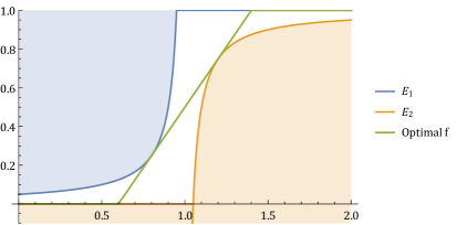
Figure 2: The forbitten regions $(E_{1})$, $(E_{2})$ and the optimal function $f$ for $a=2$, $\delta=1/10$.

In it is not difficult to see that the any function $f:[0,a]\to[0,1]$ that avoids $(E_{1})$ and $(E_{2})$ has to have at some point $\xi\in[0,a]$ a slope $f^{\prime}(\xi)$ that is at least the slope of the green line in Figure 2 which represents the line that is both targent to the boundary of $(E_{1})$ and to the boundary of $(E_{2})$. This target line can we computed in a closed form and its slope can be shown to be greater than $1/8\delta$. We leave the precise calculation as an exercise to the reader.

Inductive Step, from $\boldsymbol{d}$ to $\boldsymbol{d^{2}}$. We assume by inductive hypothesis that for any soft maximum function $\boldsymbol{f}$ in $d$ dimensions, with Lipschitz constant at most $\log(d)/8\delta$ has expected approximation loss at least $\delta$. We will then prove that for any soft maximum function $\boldsymbol{f}$ in $d^{2}$ dimensions with Lipschitz constant at most $\log(d)/8\delta$ has expected approximation loss at least $2\cdot\delta$. This in turn implies that if $\boldsymbol{f}$ has Lipschitz constant at most $2\log(d)/8\delta$ then $\boldsymbol{f}$ has expected approximation loss at least $\delta$.

Consider any soft maximum function $\boldsymbol{f}:\mathbb{R}_{+}^{d^{2}}\to\Delta_{d^{2}-1}$ and let

$$\delta^{*}=\max_{\boldsymbol{z}\in\mathbb{R}_{+}^{d^{2}}}\left\|\boldsymbol{z}\right\|_{\infty}-\langle\boldsymbol{f}(\boldsymbol{z}),\boldsymbol{z}\rangle.$$

We restrict our attention to a subspace of $\mathbb{R}_{+}^{d^{2}}$ that is produced by $\left(\mathbb{R}_{+}^{d}\right)^{2}$ by the following map $\boldsymbol{g}:\left(\mathbb{R}_{+}^{d}\right)^{2}\to\mathbb{R}_{+}^{d^{2}}$ defined as

$$g_{\ell}(\boldsymbol{x},\boldsymbol{y})=x_{\ell\bmod d}+y_{\ell\text{ div }d}.$$

We also define

$$\hat{\delta}=\max_{\boldsymbol{x},\boldsymbol{y}\in\mathbb{R}_{+}^{d}}\left\|\boldsymbol{g}(\boldsymbol{x},\boldsymbol{y})\right\|_{\infty}-\langle\boldsymbol{f}(\boldsymbol{g}(\boldsymbol{x},\boldsymbol{y})),\boldsymbol{g}(\boldsymbol{x},\boldsymbol{y})\rangle.$$

On these instances of $\mathbb{R}^{d^{2}}$ we want to view the space of alternatives $[d^{2}]$ as a product space $[d]\otimes[d]$ and that’s what the mapping $\boldsymbol{g}$ is capturing. We also want to view the output distribution as a product distribution over $[d]\otimes[d]$ but since we cannot assume independence we only define the marginal distributions of $\boldsymbol{f}(\boldsymbol{z})$ to the coordinates $\ell$ that have index with the same value $\ell\bmod d$, and the coordinates $\ell$ that have the same value $\ell\text{ div }d$. We will call $\boldsymbol{q}:\mathbb{R}_{+}^{d^{2}}\to\Delta_{d}$ the marginal distribution to the coordinates $\ell$ that have index with the same value $\ell\text{ div }d$ and $\boldsymbol{r}:\mathbb{R}_{+}^{d^{2}}\to\Delta_{d}$ the marginal distribution to the coordinates $\ell$ that have the same value $\ell\bmod d$. More formally

$$q_{i}(\boldsymbol{z})=\sum_{j=1}^{d}f_{id+j}(\boldsymbol{z})$$

and $$r_{j}(\boldsymbol{z})=\sum_{i=1}^{d}f_{id+j}(\boldsymbol{z}).$$

Now it is easy to observe that

$$\left\|\boldsymbol{g}(\boldsymbol{x},\boldsymbol{y})\right\|_{\infty} =\left\|\boldsymbol{x}\right\|_{\infty}+\left\|\boldsymbol{y}\right\|_{\infty}$$

$$\text{ and }\leavevmode\nobreak\ \leavevmode\nobreak\ \leavevmode\nobreak\ \langle\boldsymbol{f}(\boldsymbol{g}(\boldsymbol{x},\boldsymbol{y})),\boldsymbol{g}(\boldsymbol{x},\boldsymbol{y})\rangle =\langle\boldsymbol{q}(\boldsymbol{g}(\boldsymbol{x},\boldsymbol{y})),\boldsymbol{x}\rangle+\langle\boldsymbol{r}(\boldsymbol{g}(\boldsymbol{x},\boldsymbol{y})),\boldsymbol{y}\rangle.$$

Hence

$$\left\|\boldsymbol{g}(\boldsymbol{x},\boldsymbol{y})\right\|_{\infty}-\langle\boldsymbol{f}(\boldsymbol{g}(\boldsymbol{x},\boldsymbol{y})),\boldsymbol{g}(\boldsymbol{x},\boldsymbol{y})\rangle=\underbrace{\left\|\boldsymbol{x}\right\|_{\infty}-\langle\boldsymbol{q}(\boldsymbol{g}(\boldsymbol{x},\boldsymbol{y})),\boldsymbol{x}\rangle}_{\delta_{1}(\boldsymbol{x},\boldsymbol{y})}+\underbrace{\left\|\boldsymbol{y}\right\|_{\infty}-\langle\boldsymbol{r}(\boldsymbol{g}(\boldsymbol{x},\boldsymbol{y})),\boldsymbol{y}\rangle}_{\delta_{2}(\boldsymbol{x},\boldsymbol{y})}$$

We now define a continuous two game with the following players:

1. the first player picks a strategy $\boldsymbol{x}\in\mathbb{R}^{d}$ and has utility function equal to $\delta_{1}(\boldsymbol{x},\boldsymbol{y})$, and

2. the second player picks a strategy $\boldsymbol{y}\in\mathbb{R}^{d}$ and has utility function equal to $\delta_{2}(\boldsymbol{x},\boldsymbol{y})$.

It is easy to see that since $\boldsymbol{f}$ is Lipschitz continuous, both $\boldsymbol{q}$ and $\boldsymbol{r}$ are continuous and this implies that $\delta_{1}$ and $\delta_{2}$ are continuous. It is well known then from the theory of continuous games that there exists a mixed Nash Equilibrium in the game that we described above [Gli52]. This means that there exists a pair of distributions $\mathcal{D}_{x}$, $\mathcal{D}_{y}$ in $\mathbb{R}^{d}$ such that

1. for every $\boldsymbol{x}^{\star}$ in the support of $\mathcal{D}_{x}$ it holds that $\boldsymbol{x}^{\star}=\operatorname*{argmax}_{\boldsymbol{x}\in\mathbb{R}^{d}}\operatorname*{{\mathbb{E}}}_{\boldsymbol{y}\sim\mathcal{D}_{y}}\left[\delta_{1}(\boldsymbol{x},\boldsymbol{y})\right]$, and

2. for every $\boldsymbol{y}^{\star}$ in the support of $\mathcal{D}_{y}$ it holds that $\boldsymbol{y}^{\star}=\operatorname*{argmax}_{\boldsymbol{y}\in\mathbb{R}^{d}}\operatorname*{{\mathbb{E}}}_{\boldsymbol{x}\sim\mathcal{D}_{x}}\left[\delta_{2}(\boldsymbol{x},\boldsymbol{y})\right]$.

Let us know define the following functions

• $\bar{\boldsymbol{q}}(\boldsymbol{x})=\operatorname*{{\mathbb{E}}}_{\boldsymbol{y}\sim\mathcal{D}_{y}}\left[\boldsymbol{q}(\boldsymbol{g}(\boldsymbol{x},\boldsymbol{y}))\right]$,

• $\bar{\boldsymbol{r}}(\boldsymbol{y})=\operatorname*{{\mathbb{E}}}_{\boldsymbol{x}\sim\mathcal{D}_{x}}\left[\boldsymbol{r}(\boldsymbol{g}(\boldsymbol{x},\boldsymbol{y}))\right]$,

• $\bar{\delta}_{1}(\boldsymbol{x})=\operatorname*{{\mathbb{E}}}_{\boldsymbol{y}\sim\mathcal{D}_{y}}\left[\delta_{1}(\boldsymbol{x},\boldsymbol{y})\right]=\left\|\boldsymbol{x}\right\|_{\infty}-\langle\bar{\boldsymbol{q}}(\boldsymbol{x}),\boldsymbol{x}\rangle$, and

• $\bar{\delta}_{2}(\boldsymbol{y})=\operatorname*{{\mathbb{E}}}_{\boldsymbol{x}\sim\mathcal{D}_{x}}\left[\delta_{2}(\boldsymbol{x},\boldsymbol{y})\right]=\left\|\boldsymbol{y}\right\|_{\infty}-\langle\bar{\boldsymbol{r}}(\boldsymbol{y}),\boldsymbol{y}\rangle$

where in the definition of the last two functions we have used the linearity of expectation. Form the existence of the Nash Equilibrium in the aforementioned continuous game we have that

$$\operatorname*{{\mathbb{E}}}_{\boldsymbol{x}\sim\mathcal{D}_{x},\boldsymbol{y}\sim\mathcal{D}_{y}}\left[\delta_{1}(\boldsymbol{x},\boldsymbol{y})+\delta_{2}(\boldsymbol{x},\boldsymbol{y})\right]=\max_{\boldsymbol{x}\in\mathbb{R}^{d}}\left\{\bar{\delta}_{1}(\boldsymbol{x})\right\}+\max_{\boldsymbol{y}\sim\mathbb{R}^{d}}\left\{\bar{\delta_{2}(\boldsymbol{y})}\right\}$$

which in turn implies the following

$$\max_{\boldsymbol{x},\boldsymbol{y}\in\mathbb{R}^{d}}\left\{\delta_{1}(\boldsymbol{x},\boldsymbol{y})+\delta_{2}(\boldsymbol{x},\boldsymbol{y})\right\}\geq\max_{\boldsymbol{x}\in\mathbb{R}^{d}}\left\{\bar{\delta}_{1}(\boldsymbol{x})\right\}+\max_{\boldsymbol{y}\sim\mathbb{R}^{d}}\left\{\bar{\delta_{2}(\boldsymbol{y})}\right\}.$$ (C.1)

Next our goal is to relate the Lipschitzness of $\boldsymbol{f}$ with the Lipschitzness of $\bar{\boldsymbol{q}}$ and $\bar{\boldsymbol{r}}$. Observe that

$$\left\|\boldsymbol{g}(\boldsymbol{x},\boldsymbol{y})-\boldsymbol{g}(\boldsymbol{x^{\prime}},\boldsymbol{y^{\prime}})\right\|_{\infty} =\left\|\boldsymbol{x}-\boldsymbol{x^{\prime}}\right\|_{\infty}+\left\|\boldsymbol{y}-\boldsymbol{y^{\prime}}\right\|_{\infty}$$ (C.2)

$$\left\|\boldsymbol{q}(\boldsymbol{g}(\boldsymbol{x},\boldsymbol{y}))-\boldsymbol{q}(\boldsymbol{g}(\boldsymbol{x^{\prime}},\boldsymbol{y^{\prime}}))\right\|_{1} \leq\left\|\boldsymbol{f}(\boldsymbol{g}(\boldsymbol{x},\boldsymbol{y}))-\boldsymbol{f}(\boldsymbol{g}(\boldsymbol{x^{\prime}},\boldsymbol{y^{\prime}}))\right\|_{1}$$ (C.3)

$$\left\|\boldsymbol{r}(\boldsymbol{g}(\boldsymbol{x},\boldsymbol{y}))-\boldsymbol{r}(\boldsymbol{g}(\boldsymbol{x^{\prime}},\boldsymbol{y^{\prime}}))\right\|_{1} \leq\left\|\boldsymbol{f}(\boldsymbol{g}(\boldsymbol{x},\boldsymbol{y}))-\boldsymbol{f}(\boldsymbol{g}(\boldsymbol{x^{\prime}},\boldsymbol{y^{\prime}}))\right\|_{1}$$ (C.4)

where the first equality follows from simple calculations and the second and third inequality follow from the known fact that the total variation distance of a distribution is lower bounded by the total variation of its marginals.

Now we remind that we have assumed that $\boldsymbol{f}$ has $(\ell_{\infty},\ell_{1})$-Lipschitz constant that is at most $L=\log(d)/8\delta$. Using the fact that the $\ell_{1}$ norm is a convex function and using the Jensen inequality we have that

$$\left\|\bar{\boldsymbol{q}}(\boldsymbol{x})-\bar{\boldsymbol{q}}(\boldsymbol{x}^{\prime})\right\|_{1} \leq\operatorname*{{\mathbb{E}}}_{\boldsymbol{y}\sim\mathcal{D}_{y}}\left[\left\|\boldsymbol{q}(\boldsymbol{x},\boldsymbol{y})-\boldsymbol{q}(\boldsymbol{x}^{\prime},\boldsymbol{y})\right\|_{1}\right]$$

$$\leq\operatorname*{{\mathbb{E}}}_{\boldsymbol{y}\sim\mathcal{D}_{y}}\left[\left\|\boldsymbol{f}(\boldsymbol{g}(\boldsymbol{x},\boldsymbol{y}))-\boldsymbol{f}(\boldsymbol{g}(\boldsymbol{x}^{\prime},\boldsymbol{y}))\right\|_{1}\right]\leq L\cdot\left\|\boldsymbol{x}-\boldsymbol{x}^{\prime}\right\|_{\infty}$$ (C.5)

where the first inequality is due to Jensen, the second inequality follows from (C.3) and the last inequality follows from the $(\ell_{\infty},\ell_{1})$-Lipschitz constant of $\boldsymbol{f}$ and (C.2). The same way we can prove the following

$$\left\|\bar{\boldsymbol{r}}(\boldsymbol{y})-\bar{\boldsymbol{r}}(\boldsymbol{y}^{\prime})\right\|_{1} \leq L\cdot\left\|\boldsymbol{y}-\boldsymbol{y}^{\prime}\right\|_{\infty}.$$ (C.6)

It hence follows that both $\bar{\boldsymbol{q}}$ and $\bar{\boldsymbol{r}}$ are soft-max functions in $d$ dimensions with Lipschitz constant at most $L=\log(d)/8\delta$. Hence from our inductive hypothesis we have that the approximation error of both $\bar{\boldsymbol{q}}$, $\bar{\boldsymbol{r}}$ is at least $\delta$, of more formally

$$\max_{\boldsymbol{x}\in\mathbb{R}^{d}}\bar{\delta_{1}}(\boldsymbol{x})\geq\delta\leavevmode\nobreak\ \leavevmode\nobreak\ \leavevmode\nobreak\ \leavevmode\nobreak\ \leavevmode\nobreak\ \leavevmode\nobreak\ \text{and}\leavevmode\nobreak\ \leavevmode\nobreak\ \leavevmode\nobreak\ \leavevmode\nobreak\ \leavevmode\nobreak\ \leavevmode\nobreak\ \max_{\boldsymbol{y}\in\mathbb{R}^{d}}\bar{\delta}_{2}(\boldsymbol{y})\geq\delta.$$

Now putting the above inequalities together with (C.1) we get that the approximation error of $\boldsymbol{f}$ is at least $2\delta$. Formally $\max_{\boldsymbol{x},\boldsymbol{y}\in\mathbb{R}^{d}}\left\{\delta_{1}(\boldsymbol{x},\boldsymbol{y})+\delta_{2}(\boldsymbol{x},\boldsymbol{y})\right\}\geq 2\delta$. This concludes the inductive step and proves our theorem.

C.2 Proof of Theorem 4.5

We set $\boldsymbol{x}=(x,0,\dots,0)^{T}$ and $\boldsymbol{y}=(y,0,\dots,0)^{T}$, with $y>x$. Then we have

$$\textsc{Exp}(\boldsymbol{x})=\left(\frac{e^{\alpha x}}{e^{\alpha x}+(d-1)},\frac{1}{e^{\alpha x}+(d-1)},\cdots,\frac{1}{e^{\alpha x}+(d-1)}\right)^{T}$$

$$\textsc{Exp}(\boldsymbol{y})=\left(\frac{e^{\alpha y}}{e^{\alpha x}+(d-1)},\frac{1}{e^{\alpha y}+(d-1)},\cdots,\frac{1}{e^{\alpha y}+(d-1)}\right)^{T}.$$

Since $y>x$, we compute

$$\left\|\textsc{Exp}(\boldsymbol{x})-\textsc{Exp}(\boldsymbol{y})\right\|_{1} =\left(\frac{e^{\alpha y}}{e^{\alpha y}+(d-1)}-\frac{e^{\alpha x}}{e^{\alpha x}+(d-1)}\right)$$

$$-(d-1)\left(\frac{1}{e^{\alpha y}+(d-1)}-\frac{1}{e^{\alpha x}+(d-1)}\right)$$

and $\left\|\boldsymbol{x}-\boldsymbol{y}\right\|_{p}=y-x$. Now let

$$h(z)=\frac{e^{\alpha z}}{e^{\alpha z}+(d-1)}-(d-1)\frac{1}{e^{\alpha y}+(d-1)}=\frac{e^{\alpha z}-(d-1)}{e^{\alpha z}+(d-1)}$$

our goal to maximize, with respect to $x,y\in\mathbb{R}_{+}$ with $y\geq x$, the ratio

$$\frac{\left\|\textsc{Exp}(\boldsymbol{x})-\textsc{Exp}(\boldsymbol{y})\right\|_{1}}{\left\|\boldsymbol{x}-\boldsymbol{y}\right\|_{p}}=\frac{h(y)-h(x)}{y-x}.$$

Because of the mean value theorem this is equivalent with maximum with respect to $z\in\mathbb{R}_{+}$ the derivative of $h$, $h^{\prime}(z)$. But we have

$$h^{\prime}(z)=\frac{\alpha e^{\alpha z}\left(e^{\alpha z}+(d-1)\right)-\alpha e^{\alpha z}\left(e^{\alpha z}-(d-1)\right)}{\left(e^{\alpha z}+(d-1)\right)^{2}}=2\alpha\frac{e^{\alpha z}(d-1)}{\left(e^{\alpha z}+(d-1)\right)^{2}}.$$

Now we set $z=\frac{\log d}{\alpha}$ and we get for $d>10$

$$h^{\prime}\left(\frac{\log d}{\alpha}\right)=2\alpha\frac{d(d-1)}{(2d-1)^{2}}\leq\frac{\alpha}{2}.$$

Finally since the absolute approximation error of the exponential mechanism with parameter $\alpha$ is $\log d/\alpha$, to get $\delta$ absolute error we have to set $\alpha=\log d/\delta$ and hence for this regime

$$c\geq\frac{\log d}{2\delta}$$

and the proof of the theorem is completed.

Appendix D Application to Mechanism Design

In this section we show how to design a digital auction with limited supply and worst case guarantees. As we will see to do so we need to relax the incentive compatibility constraints to approximate incentive compatibility in the framework as in [MT07]. In this setting we fix an anonymous price for all the agents regardless of whether their values follow the same distribution of not. In this case we show that we can extract almost the optimal revenue among all the fixed price auctions.

Compared to the results of [MT07] and [BBHM05] our mechanism can interpolate between both of the results. Most importantly our results, in contrast to both [MT07] and [BBHM05] achieves a worst case guarantee instead of a guarantee in expectation or with high probability. Another improvement of our result is that it holds even if we do not assume unlimited supply but we only have finite supply of the item to sell.

We start with the next Section D.1 with the basic definitions and formulation of the mechanism and auction design problem.

D.1 Definitions and Preliminaries

We first give some necessary basic definitions of design auctions for selling $k$ identical items to $n$ independent bidders with unit demand valuations.

Items. We have $k$ identical items for sell.

Bidders. We have $n$ independent bidders with unit demand valuations over the $k$ item to sell. The bidders are clustered in $t$ classes and let $t(i)$ be the class of bidder $i$. The value of bidder $i\in[n]$ for any of the items is $v_{i}\in[0,H]$ where $H$ is the maximum possible value that we assume to be known. We also assume that $v_{i}$ it is drawn from a distribution $\mathcal{F}_{t(i)}$. We assume that all the random variables $v_{i}$ are independent from each other.

Mechanism. A mechanism $M$ is a function $M:\mathbb{R}_{+}^{n}\to\Delta_{n}^{k}\times\mathbb{R}_{+}^{n}$ that takes as input the bid of the players and outputs $k$ probability distributions $\boldsymbol{A}=(\boldsymbol{a}_{1},\dots,\boldsymbol{a}_{k})\in\Delta_{n}^{k}$ over the bidders that determines the probability that each bidder is going to receive the item $j$, together with a non-negative value $p_{i}$ for every bidder $i$ that determines the money bidder $i$ will pay. We write $M(\boldsymbol{v})=(\boldsymbol{A},\boldsymbol{p})$ and we call $\boldsymbol{A}\in\Delta_{n}^{k}$ the allocation rule of the mechanism $M$ and $\boldsymbol{p}$ the payment rule of $M$.

Bidders Utility. We assume that the bidders are unit-demand and they have quasi-linear utility, i.e. that the utility function $u_{i}:\Delta_{n}\times\mathbb{R}_{+}^{n}\to\mathbb{R}$ of each bidder is equal to $u_{i}(\boldsymbol{A},\boldsymbol{p})=\max_{j}(a_{ij}v_{i})-p_{i}$.

Revenue Objective. For every mechanism $M$ the revenue $\textsc{Rev}(M,\boldsymbol{v})$ the designer gets in input $\boldsymbol{v}$ is equal to $\textsc{Rev}(M,\boldsymbol{v})=\sum_{i\in[n]}p_{i}$ where $\boldsymbol{p}$ is the vector of prices that the mechanism $M$ assigns to the agents in input $\boldsymbol{v}$. By $\textsc{Rev}(M)$ we denote the expected value of the mechanism $M$ when the values $\boldsymbol{v}$ are drawn from their distributions, i.e. $\textsc{Rev}(M)=\operatorname*{{\mathbb{E}}}\left[\textsc{Rev}(M,\boldsymbol{v})\right]$.

Incentive Compatibility. A mechanism $M$ is called dominant strategy incentive compatible (DSIC) or simply incentive compatible (IC) if the bidders cannot increase their revenue by misreporting their bids. More precisely we say that $M$ satisfies incentive compatibility if for every bidder $i$

$$u_{i}(M(v_{i},\boldsymbol{v}_{-i}))\geq u_{i}(M(v^{\prime}_{i},\boldsymbol{v}_{-i})) \leavevmode\nobreak\ \leavevmode\nobreak\ \leavevmode\nobreak\ \leavevmode\nobreak\ \leavevmode\nobreak\ \leavevmode\nobreak\ \leavevmode\nobreak\ \leavevmode\nobreak\ \forall\leavevmode\nobreak\ v_{i},v^{\prime}_{i},\boldsymbol{v}_{-i}.$$ (D.1)

Also we say that $M$ is $\varepsilon$-incentive compatible if for every bidder $i$

$$u_{i}(M(v_{i},\boldsymbol{v}_{-i}))\geq\cdot u_{i}(M(v^{\prime}_{i},\boldsymbol{v}_{-i}))-\varepsilon \leavevmode\nobreak\ \leavevmode\nobreak\ \leavevmode\nobreak\ \leavevmode\nobreak\ \leavevmode\nobreak\ \leavevmode\nobreak\ \leavevmode\nobreak\ \leavevmode\nobreak\ \forall\leavevmode\nobreak\ v_{i},v^{\prime}_{i},\boldsymbol{v}_{-i}.$$ (D.2)

Individual Rationality. We say that a mechanism $M$ satisfies individual rationality if for every bidder $i$ $u_{i}(M(\boldsymbol{v}))\geq 0$ for all $\boldsymbol{v}\in\mathbb{R}_{+}^{n}$.

Optimal Revenue over a Ground Set. Let $\mathcal{M}=\{M_{1},\dots,M_{d}\}$ be a set of mechanisms which we call ground set, we define the maximum revenue of $\mathcal{M}$ at input $\boldsymbol{v}$ as $\textsc{OptRev}(\mathcal{M},\boldsymbol{v})=\max_{M\in\mathcal{M}}\textsc{Rev}(M,\boldsymbol{v})$. Also we define maximum expected revenue achievable by any mechanism in $\mathcal{M}$ to be $\textsc{OptRev}(\mathcal{M})=\max_{M\in\mathcal{M}}\textsc{Rev}(M)$.

The mechanisms that we describe in this section involve a smooth selection of a mechanism among the mechanisms in a carefully chosen ground set of incentive compatible and individual rational mechanisms $\mathcal{M}$.

Soft Maximizer Mechanism. Let $\mathcal{M}=\{M_{1},\dots,M_{d}\}$ be a ground set of incentive compatible and individually rational mechanism. We define the mechanism $Q[\mathcal{M},\boldsymbol{f}]$ to be the mechanism that chooses one of the mechanisms in $[d]$ randomly from the probability distribution that output the soft maximum function $\boldsymbol{f}$ with input the vector $\boldsymbol{x}=(\textsc{Rev}(M_{1},\boldsymbol{v}),\dots,\textsc{Rev}(M_{d},\boldsymbol{v}))$.

The following lemma proves the incentive compatibility properties of the mechanism $Q[\mathcal{M},\boldsymbol{f}]$ when the $\boldsymbol{f}$ satisfies some stability properties. For a proof of this lemma we refer to the proof of Lemma 3 in McSherry and Talwar [MT07].

Lemma D.1.

Let the bidders valuations come from the interval $[0,H]$, let also $\mathcal{M}=\{M_{1},\dots,M_{d}\}$ be a ground set of incentive compatible and individually rational mechanism and $\boldsymbol{f}$ be a soft maximum function that is $(\ell_{p},\ell_{1})$-Lipschitz with Lipschitz constant $L=\varepsilon/S_{\chi}(\textsc{Rev})$. Then the mechanism $Q[\mathcal{M},\boldsymbol{f}]$ is individually rational and $\varepsilon$-incentive compatible.

D.2 Selling Digital Goods with Anonymous Price

The single parameter auctions are arguably the most classical setting in the mechanism design literature. Myerson, in his seminal work [Mye81], proved that among all the possible auction designs the revenue is maximized by a second price auction with reserve price. The basic assumptions of his framework though is the assumption that the auctioneer has a prior belief for the values of the different bidders and she tries to maximize her expected revenue in this Bayesian setting. This assumption is the major milestone in applying the Myerson’s auction in practice. Trying to relax this assumption, a line of theoretical computer science work studied the maximization of revenue when we only have access to samples that come from the bidders distribution and not access to the entire distribution [RTCY12, DRY15, CR14, MR15, DHP16, CD17]. Although these works make a very good progress on understanding the optimal auctions and make them more practical there are still some drawbacks that make these auctions not applicable in practice.

1. Buyers may strategize in the collection of samples. If the buyers know that the seller is going to collect samples to estimate the optimal auction to run then they have incentives to strategize so that the seller chooses lower prices and hence they get more utility.

2. Constant approximation is not always a satisfying guarantee. The constant approximation is a worst case guarantee and hence the constant approximation mechanisms might fail to get almost optimal revenue even in the instances where this is easy. A popular alternative in practical applications of mechanism design is to choose the optimal from a set of simple mechanisms.

Because of these reasons, 1. and 2., the implementation and the theoretical guarantees of the mechanism $Q[\mathcal{M},\boldsymbol{f}]$ becomes a relevant problem. The ground set of mechanisms that we consider in this section is a subset of the second price selling separately auctions with a single reserved price, which we call set of anonymous auctions and we denote by $\mathcal{M}_{A}$. We are now ready to prove the main result of this section.

Theorem D.2.

Consider a $k$ identical item auction instance with unit demand bidder’s and values in the range $[0,H]$. Then there exists a ground set of mechanisms $\hat{\mathcal{M}}\subseteq\mathcal{M}_{A}$ such that for all $\boldsymbol{v}\in[0,H]^{n}$ and for any of the possible outputs of $Q\left[\hat{\mathcal{M}},\textsc{PLSoftMax}^{\eta}\right]$ with input $\boldsymbol{v}$ it holds that

$$\textsc{Rev}(Q\left[\hat{\mathcal{M}},\textsc{PLSoftMax}^{\eta}\right],\boldsymbol{v})\geq(1-\delta)\textsc{OptRev}(\mathcal{M}_{A},\boldsymbol{v})-4\left(\frac{1}{\delta}-1\right)\frac{H}{\varepsilon}$$

where $\textsc{PLSoftMax}^{\eta}$ is the soft maximum function defined in (4.1) with parameter such that PLSoftMax is $\varepsilon$-Lipschitz in Total Variation Distance. Moreover $Q[\hat{\mathcal{M}},\textsc{PLSoftMax}]$ is individually rational and $\varepsilon\cdot H$-incentive compatible.

Proof.

Let $[0,H]$ be the range of prices for the single item auction. We fix a positive real number $\delta$ and we use the discretization $\mathcal{P}$ of $[0,H]$, where $\mathcal{P}=\{p_{1},\dots,p_{d}\}$ and $p_{i}=H\cdot(1-\delta)^{i}$. Let also $\alpha=p_{d}$. We are now ready to define the ground set of mechanisms $\hat{\mathcal{M}}=\{M_{1},\dots,M_{d}\}$ where $M_{i}$ is the second price auction with reserved price equal to $p_{i}$. The size of $\hat{\mathcal{M}}$ is

$$d=\log\left(\frac{\alpha}{H}\right)/\log(1-\delta)\leq 2\log\left(\frac{H}{\alpha}\right)/\delta$$

where the last inequality follows assuming that $\delta\leq 1/2$. As we described, we will run our mechanism PLSoftMax, with objective function Rev. In order to be able to apply our main theorem about the PLSoftMax mechanism we will bound the $\ell_{1}$-sensitivity of the vector $\boldsymbol{x}=(\textsc{Rev}(M_{1},\boldsymbol{v}),\dots,\textsc{Rev}(M_{d},\boldsymbol{v}))$ with respect the change of the bid of one agent. Hence we need to bound the quantity

$$\sum_{i=1}^{d}\left|\textsc{Rev}(M_{i},(v_{i},\boldsymbol{v}_{-i}))-\textsc{Rev}(M_{i},(v^{\prime}_{i},\boldsymbol{v}_{-i}))\right|\leq(1-\delta)\frac{H}{\delta}.$$

This inequality holds because for every agent $i$ the total change that agent $i$ can make in the revenue objective of all the alternatives is at most

$$\sum_{i=1}^{d}(1-\delta)^{i}H\leq\left(\frac{1}{\delta}-1\right)H,$$

which implies that for our setting $S_{1}(\textsc{Rev})\leq\left(\frac{1}{\delta}-1\right)H$.

The approximation loss of our mechanism has three components: (1) we loose $\delta\mathrm{OPT}$ because of the discretization of the price of every item, (2) we loose $\alpha$ from every item because we need the ground set to be finite and (3) we loose $\eta$ because we use the soft maximization algorithm $\textsc{PLSoftMax}^{\eta}$. For the last part and since we need $\textsc{PLSoftMax}^{\eta}$ to be $\varepsilon$-Lipschitz in total variation distance we have that

$$\varepsilon=\frac{4}{\eta}S_{1}(\textsc{Rev})\leq\frac{4}{\eta}\left(\frac{1}{\delta}-1\right)H\implies\eta\leq\frac{4}{\varepsilon}\left(\frac{1}{\delta}-1\right)H.$$

Finally applying Theorem 4.3 the theorem follows. ∎

If we assume that $H=O(1)$ then by setting $\delta\leftarrow\frac{1}{\sqrt{\mathrm{OPT}}}$ and $\varepsilon\leftarrow\varepsilon\cdot H$ we recover the result of [BBHM05], with relaxed incentive compatibility, but even in the case of limited supply and having a worst case guarantee.

Corollary D.3.

Consider a $k$ identical item auction instance with unit demand bidder’s and values in the range $[0,H]$. If we fix $H$ then there exists a mechanism $M$ such that for any $\boldsymbol{v}\in[0,H]^{n}$, for all $\boldsymbol{v}\in[0,H]^{n}$ and for any of the possible outputs of $M$ with input $\boldsymbol{v}$ it holds that

$$\textsc{Rev}(M,\boldsymbol{v})\geq\textsc{OptRev}(\mathcal{M}_{A})-O\left(\frac{1}{\varepsilon}\sqrt{\textsc{OptRev}(\mathcal{M}_{A})}\right)$$

where $M$ is individually rational and $\varepsilon$-incentive compatible.

Another corollary can be directly derived by applying a discretized version of the Theorem 9 of [MT07] but replacing the exponential mechanism with the PLSoftMax mechanism. Then as we explained in Section 4 the guarantees will hold in the worst case and not in expectation.

Corollary D.4.

Consider a $k$ identical item auction instance with unit demand bidder’s and values in the range $[0,H]$. If we fix $H$ then there exists a mechanism $M$ such that for any $\boldsymbol{v}\in[0,H]^{n}$, for all $\boldsymbol{v}\in[0,H]^{n}$ and for any of the possible outputs of $M$ with input $\boldsymbol{v}$ it holds that

$$\textsc{Rev}(M,\boldsymbol{v})\geq\textsc{OptRev}(\mathcal{M}_{A})-O\left(\frac{1}{\varepsilon}\log\left(\textsc{OptRev}(\mathcal{M}_{A})\cdot k\right)\right)$$

where $M$ is individually rational and $\varepsilon$-incentive compatible.

As we can see Corollary D.3 and Corollary D.4 are not directly comparable since in Corollary D.4 the $\log(k)$ factor in the approximation error appears that misses from Corollary D.3.

Appendix E Maximization of Submodular Functions

In this section we consider the problem of differential privately maximizing a submodular function, under cardinality constraints. For this problem we apply the power mechanism and we compare our results with the state of the art work of Mitrovic et al. [MBKK17]. We observe that when the input data set is only $O(1)$-multiplicative insensitive power mechanism has an error that is asymptotically smaller than the corresponding error from the state of the art algorithm of Mitrovic et al. [MBKK17]. This result is formally stated in Corollary 6.6.

As discussed in Section 6.2.1, to solve the submodular maximization under cardinality constraints we use the Algorithm 1 of [MBKK17], where we replace the exponential mechanism in the soft maximization step with the power mechanism.

Algorithm 1 (Algorithm 1 of [MBKK17]):

Input: submodular function $h$, soft maximization function $\boldsymbol{g}$, $k\in\mathbb{N}$.

Output: $S\subseteq\mathcal{D}$ such that $\left|S\right|=k$.

1. Initialize $S_{o}=\emptyset$. Let $\left|\mathcal{D}\right|=d$ and $\mathcal{D}=\{v_{1},\dots,v_{d}\}$.

2. For $i\in[k]$:

   1. Define $q_{i}:\mathcal{D}\setminus S_{i-1}\to\mathbb{R}$ as

      $$q_{i}(v)=h(S_{i-1}\cup\{v\})-f(S_{i-1}).$$

   2. Pick $u_{i}\in\mathcal{D}$ from the probability distribution

      $$\boldsymbol{g}\left(q_{i}(v_{1}),\dots,q_{i}(v_{d})\right).$$

   3. $S_{i}\leftarrow S_{i}\cup\{u_{i}\}$.

3. Return $S_{k}$.

To analyze Algorithm 1 we need the following result for compositions of differentially private algorithms.

Composition of Differentially Private Algorithms. An algorithm $A$ is a composition of $k$ algorithms $A_{1},\dots,A_{k}$ if the output of $A(\boldsymbol{v})$ is a function only of the outputs $A_{1}(\boldsymbol{v}),\dots,A_{k}(\boldsymbol{v})$.

The following theorem bounds the privacy of $A(\boldsymbol{v})$ as a function of the privacy of $A_{1}(\boldsymbol{v}),\dots,A_{k}(\boldsymbol{v})$.

Theorem E.1 ([DRV10]).

Let $A_{1},\dots,A_{k}$ be differentially private algorithms with parameters $(\varepsilon^{\prime},\delta^{\prime})$. Let also $A$ a composition of $A_{1},\dots,A_{k}$. Then, $A$ satisfies $(\varepsilon,\delta)$-differential privacy with

1. $\varepsilon=k\varepsilon^{\prime}$ and $\delta=k\delta^{\prime}$,

2. $\varepsilon=\frac{1}{2}k^{2}\varepsilon^{\prime 2}+\sqrt{2\log(1/\eta)}\varepsilon^{\prime}$ and $\delta=\eta+k\delta^{\prime}$ for any $\eta>0$.

We are now ready to prove Theorem 6.4.

Proof of Theorem 6.4..

The privacy guarantee easily follows from the composition properties of differentially private mechanisms that we present in Theorem E.1.

Let $S^{*}$ be the set of the optimal solution, $S_{i}$ be the set that the algorithm has in the $i$th iteration and $v_{i}$ the $i$th element that our algorithm chose. We have that

$$\operatorname*{{\mathbb{E}}}[ h(S_{i}\cup\{v_{i}\})-h(S_{i})]=$$

$$=\frac{1}{1+\delta}\max_{v\in\mathcal{D}\setminus S_{i-1}}(h(S_{i}\cup\{v\})-h(S_{i}))$$

$$\geq\frac{1}{1+\delta}\frac{1}{k}\left(\sum_{v\in S^{*}}(h(S_{i}\cup\{v\})-h(S_{i}))\right)$$

$$\geq\frac{1}{1+\delta}\frac{1}{k}(h(S^{*}\cup S_{i-1})-h(S_{i-1}))$$

$$\geq\frac{1}{1+\delta}\frac{1}{k}(\mathrm{OPT}-h(S_{i-1})).$$

Therefore

$$\mathrm{OPT}-\operatorname*{{\mathbb{E}}}[h(S_{i})]\leq\left(1-\frac{1}{1+\delta}\frac{1}{k}\right)^{i}\mathrm{OPT}.$$

From which we conclude

$$\operatorname*{{\mathbb{E}}}[h(S_{k})] \geq\left(1-\left(1-\frac{1}{1+\delta}\frac{1}{k}\right)^{k}\right)\mathrm{OPT}$$

$$\geq\left(1-\frac{1}{\exp(1/(1+\delta))}\right)\mathrm{OPT}.$$

and hence the theorem follows. ∎

Next our goal is to compare Theorem 8 of [MBKK17] with Theorem 6.4. We illustrate the difference between power and exponential mechanism showing an improvement over the state of the art algorithm of [MBKK17].

Lemma E.2.

Let $\delta_{\textsc{Pow}}$ be the approximation loss of Pow assuming that the input data set is $t$-multiplicative insensitive, then $\delta_{\textsc{Pow}}\leq\min\left\{\frac{1}{e}+\frac{2\sqrt{k}\log d}{t\varepsilon}\frac{S_{\infty}(h)}{\mathrm{OPT}},1\right\}$.

Proof.

From Theorem 6.4 we have that

$$\delta_{\textsc{Pow}} =\min\left\{\exp\left(-\left(1-\frac{S_{\infty}(h)}{\mathrm{OPT}}\right)^{\frac{2\sqrt{k}\log d}{\varepsilon}}\right),1\right\}$$

$$\leq\min\left\{\exp\left(-\left(1-\frac{2\sqrt{k}\log d}{\varepsilon}\frac{S_{\infty}(h)}{\mathrm{OPT}}\right)\right),1\right\}$$

$$=\frac{1}{e}\min\left\{\exp\left(\frac{2\sqrt{k}\log d}{\varepsilon}\frac{S_{\infty}(h)}{\mathrm{OPT}}\right),e\right\}$$

Now if $\frac{2\sqrt{k}\log d}{\varepsilon}\frac{S_{\infty}(h)}{\mathrm{OPT}}\geq 1$ then $\delta_{\textsc{Pow}}=1$ and hence, we can assume that $\frac{2\sqrt{k}\log d}{\varepsilon}\frac{S_{\infty}(h)}{\mathrm{OPT}}\leq 1$. But for any $z\leq 1$ it is easy to see that $e^{z}\leq 1+ez$ and hence

$$\delta_{\textsc{Pow}} \leq\frac{1}{e}\min\left\{1+e\frac{2\sqrt{k}\log d}{\varepsilon}\frac{S_{\infty}(h)}{\mathrm{OPT}},e\right\}$$

and the lemma follows. ∎

Now combining Theorem 6.4 and Lemma E.2 we can prove Corollary 6.6 which clearly illustrates the comparison of the performance of power and exponential mechanism. From Corollary 6.6 we observe that the approximation loss using the exponential mechanism is a $O(\sqrt{k})$ factor larger than the approximation loss using the power mechanism. Hence Corollary 6.6 improves over the state of the art differentially private algorithms for submodular optimization.

We can use the same ideas as in Theorem 6.4 and Corollary 6.6 to improve the results for maximization of submodular functions with more general matroid constraints of [MBKK17].

Appendix F Experiments on Large Real-World Data Sets

  Remark. In the main part we accidentally refer to Appendix F both for the theoretical and the practical results about differentially private submodular maximization. Please look at the Appendix E for the details on the theoretical part and in this section for the details in the experiments part.  

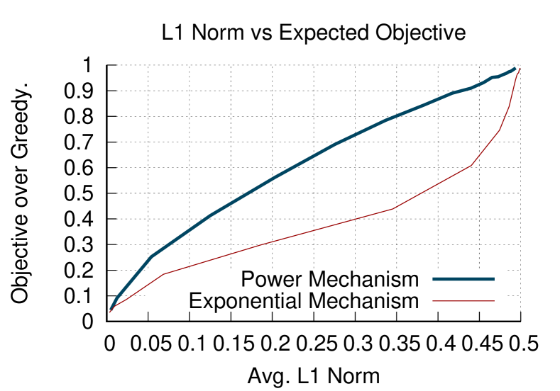
(a) $\ell_{1}$ Distance

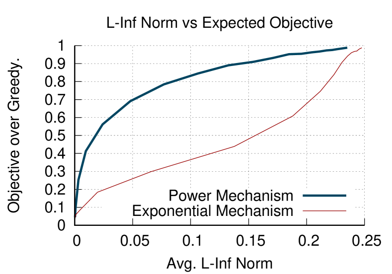
(b) $\ell_{\infty}$ Distance

Figure 3: Robustness vs objective value in the submodular maximization with cardinality constraint $k=10$. The y-axis shows the ration of the average objective obtained vs the (non-private) greedy algorithm. The x-axis represent the sensitivity to the manipulation test of the value of the first element selected.

We now empirically validate our results for submodular maximization. In our experiments we used a publicly available data-set to create a max-k-coverage instance similarly to prior work [EMZ17]. In a coverage instance we are given a family $N$ of sets over a ground set $U$ and we want to find $k$ sets from $N$ with maximum size of their union (which is a monotone submodular maximization problem under cardinality constraint). We created the coverage instance from the DBLP co-authorship network of computer scientists by extracting, for each author, the set of her coauthors. The ground set is the set of all authors in DBLP. There are $\sim 300$ thousands sets over $\sim 300$ thousands elements for a total sum of sizes of all sets of $1.0$ million. Then we ran the (non-private) greedy submodular maximization algorithm to obtain a (baseline) upperbound on the solution (notice that computing the actual optimum is NP-Hard). Then we compared the objective value obtained by private greedy algorithm for submodular maximization using the exponential mechanism (as described in Algorithm 1 in [MBKK17]) and using the power mechanism as soft-max, for different values of the parameter $\alpha$ in the two methods. We used $k=10$ as the cardinality of the output in our experiment.

To evaluate empirically the smoothness of the mechanism we performed a manipulation test on the data. We manipulated the coverage instance removing, independently, each element of the ground set with probability $1/1000$. Then, for a fixed mechanism and parameter setting, we compared the probability distribution of the first set selected by the algorithm in the manipulated instance vs in the original instance (we used the $\ell_{1}$ and $\ell_{\infty}$ distance of the distributions). Finally, we ran each configuration of the experiment (i.e., a mechanism and a parameter) $100$ times and reported the average objective in the original dataset (over the objective of non-private greedy) and average distance between the distributions obtained over the original and manipulated datasets. Figures 3(a) and 3(b) report the results for $k=10$ in the DBLP instance. Notice that we observe that for the same level of sensitivity to manipulation (both in $l_{1}$ and $l_{\infty}$ norm) the power mechanism obtains significantly more objective value in this problem as well (y-axis reports the average ratio of the objective obtained vs that of the non-private algorithm). This confirms our theoretical results for submodular maximization.

Appendix G Loss Function For Multi-class Classification

Before presenting our loss function that can be used for multi-class classification we present a proof of Lemma 6.7. Due to a minor typo in the presentation of the Lemma in the main part of the paper we restate the Lemma here corrected.

Lemma G.1 (Lemma 6.7).

Let $h(\cdot)=\mathrm{sparsegen}\text{-}\mathrm{lin}(\cdot)$ be the generalization of $\mathrm{sparsemax}(\cdot)$ function, then there exist $\boldsymbol{x},\boldsymbol{y}\in\mathbb{R}^{d}$ such that $\left\|h(\boldsymbol{x})-h(\boldsymbol{y})\right\|_{1}\geq\frac{1}{2}d^{1-1/q}\left\|\boldsymbol{x}-\boldsymbol{y}\right\|_{q}$.

Proof of Lemma 6.7..

We set $\boldsymbol{x}=\boldsymbol{0}$ and $\boldsymbol{y}$ such that $y_{i}=2/d$ for $i\leq d/2$ and $y_{i}=0$ otherwise. Doing simple calculations we get that $h(\boldsymbol{x})=(1/d)\cdot\boldsymbol{1}$, whereas $h_{i}(\boldsymbol{y})=2/d$ for $i\leq d/2$ and $h_{i}(\boldsymbol{y})=0$ otherwise. Hence we have $\left\|h(\boldsymbol{x})-h(\boldsymbol{y})\right\|_{1}=1$ and

$$\left\|\boldsymbol{x}-\boldsymbol{y}\right\|_{q}=(2/d)^{1-1/q}\leq 2/d^{1-1/q}$$

and the lemma follows. ∎

In this section, we show how our mechanism can be used in multi-class classification by proposing the corresponding loss function.

First, we note that the $\mathcal{L}_{\mathrm{sparsegen}\text{-}\mathrm{lin},\mathrm{hinge}}$ loss function defined in [MA16] can be used as a loss function for any soft-max function that satisfies: (1) permutation invariance, (2) $\delta$-worst-case approximation additive loss, where we have to set $\delta=1-\lambda$. The main issue of this loss function is that it does not take into account specific structural properties of the soft-max function used. For this reason, we propose an alternative loss function.

A loss function that corresponds to PLSoftMax with parameter $\delta$ is a function $L:\mathbb{R}^{d}\times\Delta_{d}\to\mathbb{R}_{+}$ such that for any $\boldsymbol{x}\in\mathbb{R}^{d}$ and $\boldsymbol{q}\in\Delta_{d}$, it holds that $L(\boldsymbol{x};\boldsymbol{q})=0\Leftrightarrow\textsc{PLSoftMax}^{\delta}(\boldsymbol{x})=\boldsymbol{q}$. Our loss function has three components: (1) $L_{ord}$ is minimized only when the ordering of $\boldsymbol{x}$ is the same as the ordering of $\boldsymbol{q}$, (2) $L_{supp}$ is minimized when the coordinates of $\boldsymbol{x}$ that are within $\delta$ from $\left\|\boldsymbol{x}\right\|_{\infty}$ correspond to the coordinates $i$ such that $q_{i}>0$, and (3) $L_{sqr}$ minimizes the error between $\textsc{PLSoftMax}^{\delta}(\boldsymbol{x})$ and $\boldsymbol{q}$ assuming they have the same order. Finally, our loss function $L_{\textsc{PLSoftMax}}$ is the sum of these three components, i.e. $L_{\textsc{PLSoftMax}}=L_{ord}+L_{supp}+L_{sqr}$.

Order Regularization. For every $\boldsymbol{q}\in\Delta_{d}$, let $\pi_{\boldsymbol{q}}$ be the permutation of the coordinates $[d]$ such that $q_{\pi_{\boldsymbol{q}}(1)}\geq\cdots\geq q_{\pi_{\boldsymbol{q}}(d)}$, then

$$L_{ord}(\boldsymbol{x};\boldsymbol{q})=\sum_{i=1}^{d-1}\max\{x_{\pi_{\boldsymbol{q}}(i+1)}-x_{\pi_{\boldsymbol{q}}(i+1)},0\}.$$

Support Regularization. Let $\boldsymbol{q}\in\Delta_{d}$, let $S\subseteq[d]$ be the subset of the coordinates $[d]$ such that $i\in S\Leftrightarrow q_{i}>0$, let also $\delta$ be the parameter of PLSoftMax, then

$$L_{supp}(\boldsymbol{x};\boldsymbol{q})=\sum_{i\in S}\max\{x_{\pi_{\boldsymbol{q}}(1)}-x_{i}-\delta,0\}+\sum_{i\in[d]\setminus S}\max\{x_{i}-x_{\pi_{\boldsymbol{q}}(1)}+\delta,0\}.$$

Square Loss. Let $\boldsymbol{q}\in\Delta_{d-1}$, then

$$L_{sqr}(\boldsymbol{x};\boldsymbol{q})=\left\|\boldsymbol{q}-\frac{1}{\delta}\boldsymbol{P}_{\pi_{\boldsymbol{q}}}^{-1}\boldsymbol{SM}_{(k_{\boldsymbol{q}},d)}\boldsymbol{P}_{\pi_{\boldsymbol{q}}}\boldsymbol{x}-\boldsymbol{P}_{\pi_{\boldsymbol{q}}}^{-1}\boldsymbol{u}^{(k_{\boldsymbol{q}})}\right\|_{2}^{2}.$$

The main properties of the loss function $L_{\textsc{PLSoftMax}}$ are summarized in Proposition 6.8. This proposition suggests that $L_{\textsc{PLSoftMax}}$ can be used as a meaningful loss function in multiclass classification.

Proof of Proposition 6.8..

The property (1) follows directly from the fact that $L_{\textsc{PLSoftMax}}$ is a sum of non-negative terms. Also observe that: (i) $L_{ord}=0$ if and only if the order of the coordinates of the vector $\boldsymbol{x}$ agrees with the order of the coordinates of $\boldsymbol{q}$, and (ii) $L_{supp}=0$ if and only if the only coordinates that are $\delta$-close to $\left\|\boldsymbol{x}\right\|_{\infty}$ are the coordinates for which $q_{i}>0$. Using (i) and (ii) together with $L_{sqr}=0$ we can see that the property (2) of Proposition 6.8 is implied. Property (3) follows again easily from the fact that the maximum of two convex function is convex and the sum of convex functions is also convex. ∎

References

• [BBHM05] M-F Balcan, Avrim Blum, Jason D Hartline, and Yishay Mansour. Mechanism design via machine learning. In Foundations of Computer Science, 2005. FOCS 2005. 46th Annual IEEE Symposium on, pages 605–614. IEEE, 2005.
• [Bol68] Ludwig Boltzmann. Studien uber das gleichgewicht der lebenden kraft. Wissenschafiliche Abhandlungen, 1:49–96, 1868.
• [Bri90a] John S. Bridle. Probabilistic interpretation of feedforward classification network outputs, with relationships to statistical pattern recognition. In Françoise Fogelman Soulié and Jeanny Hérault, editors, Neurocomputing, pages 227–236, Berlin, Heidelberg, 1990. Springer Berlin Heidelberg.
• [Bri90b] John S. Bridle. Training stochastic model recognition algorithms as networks can lead to maximum mutual information estimation of parameters. In D. S. Touretzky, editor, Advances in Neural Information Processing Systems 2, pages 211–217, 1990.
• [CD17] Yang Cai and Constantinos Daskalakis. Learning multi-item auctions with (or without) samples. arXiv preprint arXiv:1709.00228, 2017.
• [CR14] Richard Cole and Tim Roughgarden. The sample complexity of revenue maximization. In Proceedings of the forty-sixth annual ACM symposium on Theory of computing, pages 243–252. ACM, 2014.
• [dBV15] Alexandre de Brébisson and Pascal Vincent. An exploration of softmax alternatives belonging to the spherical loss family. arXiv preprint arXiv:1511.05042, 2015.
• [DHP16] Nikhil R Devanur, Zhiyi Huang, and Christos-Alexandros Psomas. The sample complexity of auctions with side information. In Proceedings of the forty-eighth annual ACM symposium on Theory of Computing, pages 426–439. ACM, 2016.
• [DP09] Konstantinos Drakakis and BA Pearlmutter. On the calculation of the l2→ l1 induced matrix norm. International Journal of Algebra, 3(5):231–240, 2009.
• [DR14] Cynthia Dwork and Aaron Roth. The algorithmic foundations of differential privacy. Foundations and Trends in Theoretical Computer Science, 9(3–4):211–407, 2014.
• [DRV10] Cynthia Dwork, Guy N Rothblum, and Salil Vadhan. Boosting and differential privacy. In 2010 IEEE 51st Annual Symposium on Foundations of Computer Science, pages 51–60. IEEE, 2010.
• [DRY15] Peerapong Dhangwatnotai, Tim Roughgarden, and Qiqi Yan. Revenue maximization with a single sample. Games and Economic Behavior, 91:318–333, 2015.
• [EMZ17] Alessandro Epasto, Vahab Mirrokni, and Morteza Zadimoghaddam. Bicriteria distributed submodular maximization in a few rounds. In SPAA. ACM, 2017.
• [GBC16] Ian Goodfellow, Yoshua Bengio, and Aaron Courville. Deep Learning. MIT Press, 2016.
• [Gib02] J.W. Gibbs. Elementary Principles in Statistical Mechanics: Developed with Especial Reference to the Rational Foundations of Thermodynamics. C. Scribner’s sons, 1902.
• [Gli52] Irving L Glicksberg. A further generalization of the kakutani fixed point theorem, with application to nash equilibrium points. Proceedings of the American Mathematical Society, 3(1):170–174, 1952.
• [HK12] Zhiyi Huang and Sampath Kannan. The exponential mechanism for social welfare: Private, truthful, and nearly optimal. In Proceedings of the 2012 IEEE 53rd Annual Symposium on Foundations of Computer Science, FOCS ’12, page 140–149, USA, 2012. IEEE Computer Society.
• [HO10] Julien M Hendrickx and Alex Olshevsky. Matrix p-norms are np-hard to approximate if $p\neq 1,2,\infty$. SIAM Journal on Matrix Analysis and Applications, 31(5):2802–2812, 2010.
• [JJ94] Michael I. Jordan and Robert A. Jacobs. Hierarchical mixtures of experts and the em algorithm. Neural Comput., 6(2):181–214, March 1994.
• [LCA+18] Anirban Laha, Saneem Ahmed Chemmengath, Priyanka Agrawal, Mitesh Khapra, Karthik Sankaranarayanan, and Harish G Ramaswamy. On controllable sparse alternatives to softmax. In Advances in Neural Information Processing Systems, pages 6422–6432, 2018.
• [Luc59] R. Duncan Luce. Individual Choice Behavior: A Theoretical Analysis. John Wiley & Sons, 1959.
• [MA16] Andre Martins and Ramon Astudillo. From softmax to sparsemax: A sparse model of attention and multi-label classification. In International Conference on Machine Learning, pages 1614–1623, 2016.
• [MB05] Frederic Morin and Yoshua Bengio. Hierarchical probabilistic neural network language model. In Aistats, volume 5, pages 246–252. Citeseer, 2005.
• [MBKK17] Marko Mitrovic, Mark Bun, Andreas Krause, and Amin Karbasi. Differentially private submodular maximization: Data summarization in disguise. In ICML, 2017.
• [MR15] Jamie H Morgenstern and Tim Roughgarden. On the pseudo-dimension of nearly optimal auctions. In Advances in Neural Information Processing Systems, pages 136–144, 2015.
• [MSC+13] Tomas Mikolov, Ilya Sutskever, Kai Chen, Greg S Corrado, and Jeff Dean. Distributed representations of words and phrases and their compositionality. In Advances in neural information processing systems, pages 3111–3119, 2013.
• [MT07] Frank McSherry and Kunal Talwar. Mechanism design via differential privacy. In Foundations of Computer Science, 2007. FOCS’07. 48th Annual IEEE Symposium on, pages 94–103. IEEE, 2007.
• [Mye81] Roger B Myerson. Optimal auction design. Mathematics of operations research, 6(1):58–73, 1981.
• [Roh00] Jiří Rohn. Computing the norm∥ a∥∞, 1 is np-hard∗. Linear and Multilinear Algebra, 47(3):195–204, 2000.
• [RTCY12] Tim Roughgarden, Inbal Talgam-Cohen, and Qiqi Yan. Supply-limiting mechanisms. In Proceedings of the 13th ACM Conference on Electronic Commerce, pages 844–861. ACM, 2012.
• [SB18] Richard S. Sutton and Andrew G. Barto. Reinforcement Learning: An Introduction. A Bradford Book, Cambridge, MA, USA, 2018.
• [THB86] Edward Charles Titchmarsh and David Rodney Heath-Brown. The theory of the Riemann zeta-function. Oxford University Press, 1986.
• [VDBB15] Pascal Vincent, Alexandre De Brébisson, and Xavier Bouthillier. Efficient exact gradient update for training deep networks with very large sparse targets. In Advances in Neural Information Processing Systems, pages 1108–1116, 2015.