Learning Disentangled Phone and Speaker Representations in a Semi-Supervised VQ-VAE Paradigm

Abstract

We present a new approach to disentangle speaker voice and phone content by introducing new components to the VQ-VAE architecture for speech synthesis. The original VQ-VAE does not generalize well to unseen speakers or content. To alleviate this problem, we have incorporated a speaker encoder and speaker VQ codebook that learns global speaker characteristics entirely separate from the existing sub-phone codebooks. We also compare two training methods: self-supervised with global conditions and semi-supervised with speaker labels. Adding a speaker VQ component improves objective measures of speech synthesis quality (estimated MOS, speaker similarity, ASR-based intelligibility) and provides learned representations that are meaningful. Our speaker VQ codebook indices can be used in a simple speaker diarization task and perform slightly better than an x-vector baseline. Additionally, phones can be recognized from sub-phone VQ codebook indices in our semi-supervised VQ-VAE better than self-supervised with global conditions.

Index Terms—  speech synthesis, disentanglement, representation learning, speaker diarization, phone recognition

1 Introduction

Rich representations of speaker identity, such as x-vectors [1], i-vectors [2], and learnable dictionary encodings (LDE) [3], are commonplace in many speech technologies ranging from speaker and language recognition, to text-to-speech (TTS) synthesis [4], and voice conversion (VC) [5]. Representations of speaker identity are also known to contain unwanted information not necessarily related to speaker voice because they often encode extra information such as recording environment, speaker emotion, speaking style, and lexical content. Machine learning methods can remove these unwanted informational factors, so that speaker representations can be made more pure. However, these techniques discard informational factors rather than storing them in separate representations. In addition, evaluation for disentanglement success has been limited to performing ad-hoc classification tasks, whereby a lowered classification accuracy indicates that information has been removed [6, 7, 8]. The ability to successfully disentangle and retain information from the speech signal has far-reaching benefits for speech processing. For example, voice conversion and voice privacy benefits from the ability to retain content while changing speaker characteristics. In text-to-speech synthesis, it is desirable to separately control factors of content, speaker, and expressive style.

In this paper, we present an end-to-end solution to disentangle sub-phone content and global-level speaker characteristics by building upon the original vector-quantized variational autoencoder (VQ-VAE) used in voice conversion. While VQ-VAE learns a type of sub-phone representation [9], the system cannot generalize well to unseen speakers or unseen content. We present our method to learn two different VQ codebooks at the same time while producing synthetic speech that is highly intelligible and with high speaker similarity in unseen conditions. We also demonstrate that the learned representations can be used in downstream tasks: phone recognition from VQ sub-phone codes, and speaker diarization from VQ speaker codes.

2 Related Work

Recent work from [10] aims to disentangle content from speaker for voice conversion tasks. While their technique does not necessarily rely on speaker labels, it does use vocal tract length perturbation (VTLP) to facilitate regularization during adversarial disentanglement. To facilitate content encoding, the encoder input uses instance normalization for each log-mel-band, for each input signal, separately. As mentioned earlier, the disentanglement success is only defined in terms of ad-hoc classification tasks. The approach does not create representations that are re-usable outside of the system.

In the VQ-VAE paradigm, learned VQ spaces result in rich continuous-valued embeddings as well as their corresponding discrete code indices. As embeddings, the learned representations can be used to condition a decoder, such as WaveRNN, locally or globally. It was previously shown that a large VQ space can learn to represent phones and sub-phones when trained with speech audio [9]. More recently, VQ-VAE has been successfully modified to learn two separate VQ spaces at the same time: F0 and sub-phones. Incorporating an additional encoder for F0 greatly improved speech synthesis quality for Japanese and Mandarin. However, the speaker representation was a one-hot encoded speaker vector or a separately obtained LDE vector [11]. Our work builds on this effort by learning the speaker VQ space during training and using it for global conditioning in the WaveRNN decoder. In addition, we demonstrate that the VQ code indices are very useful in other downstream tasks.

3 Architectures

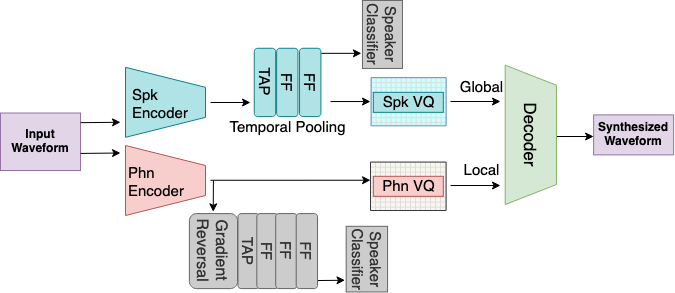
Fig. 1: System overview: Speaker VQ encodes global conditions with temporal average pooling layer (TAP). Phone VQ encodes local conditions. Colored components are described in Section 3.2, and gray components in Section 3.3

3.1 Original Self-Supervised VQ-VAE

We used the PyTorch implementation of the original VQ-VAE [9] for audio. This system is self-supervised during training as it does not require labeled data, and the learning process is governed by three terms in the loss function which balance the encoder, decoder, and VQ dictionary (Equation 1).

$$L=L_{R}+\alpha L_{VQ}+\beta L_{C}$$ (1)

First, the $L_{R}$ term is the reconstruction loss, defined as $-\log p(x|z_{q}(x))$ which is the negative log likelihood of decoder output $x$ given the output of the encoder $z(x)$ after quantization $q$. The second term $L_{VQ}$ is the VQ objective, defined as $\rVert{\mbox{sg}}[z_{e}(x)]-e\rVert_{2}^{2}$ and it is an $l_{2}$ loss which guides VQ embedding vectors $e$ towards encoder output $z_{e}(x)$. The sg term is a stop-gradient operator which effectively creates a non-updated constant. The purpose of the VQ term is to ensure that embeddings are also guided by reconstruction loss. Finally, the $L_{C}$ term is a commitment loss defined as $\rVert z_{e}(x)-{\mbox{sg}}[e]\rVert_{2}^{2}$ to ensure that the encoder commits to a VQ embedding vector $e$ and constrains how the VQ space is utilized. In our VQ-VAE implementation, the size of the sub-phone VQ codebook is 512 and each VQ embedding vector is 128-dims. The WaveRNN decoder is implemented as described in [11], and it performs local conditioning (using sub-phone VQ embeddings) as well as global conditioning (using speaker one-hot vectors).

3.2 Self-Supervised VQ-VAE + Global Conditioning

Building upon the open-source implementation provided by [11], we likewise added an encoder and VQ codebook component to the original VQ-VAE architecture. However, our addition was a VQ component that models global conditions, rather than their F0 VQ component for local conditions. To transform the encoder output into global conditions, we added a temporal average pooling layer and two feed-forward layers between the encoder and VQ dictionary (colored components of Figure 1). Our dual-encoder VQ-VAE is also self-supervised, and we have adjusted the loss function to account for the additional global terms (Equation 2).

$$L=L_{R}+\alpha(L_{VQl}+L_{Cl})+\beta(L_{VQg}+L_{Cg})$$ (2)

Similar to the original VQ-VAE defined earlier, our dual-encoder model is based on a weighted linear combination of losses. The local features ($L_{VQl}$, $L_{Cl}$) and the global features ($L_{VQg}$, $L_{Cg}$), while retaining the original reconstruction loss. In this system (+Global VQ), the sub-phone VQ codebook remains the same, while we have added a global VQ codebook of size 256, and each VQ embedding is 128-dims.

3.3 Semi-Supervised VQ-VAE + Speaker Codebook

Different from the self-supervised training method in Section 3.2, we explicitly provided speaker labels as additional information. Using speaker labels, we created two semi-supervised variants of the dual-encoder model and global conditions from Section 3.2. First, we added an auxiliary speaker classifier to the global encoder components, using VCTK speaker labels as ground truth. We experimented with two different loss functions for the speaker classifier, and we refer them as +Speaker label, Softmax for the softmax loss, and +Speaker label, A-softmax for the angular softmax loss. In each case, the classifier loss is added to the loss function of Equation 2. Finally, we added an additional auxiliary adversarial component to the phone encoder, which consists of a gradient reversal layer [12], feed-forward layers, and a speaker classifier. The purpose of this adversarial component was to encourage disentanglement of phone and speaker information. The speaker classifier for the adversarial component used softmax loss. As before, concerning the non-adversarial speaker classification task, we compare the softmax loss (+Adversarial loss, Softmax) and the angular softmax loss (+Adversarial loss, A-softmax). The semi-supervised components are shown in gray in Figure 1.

Table 1: Speech synthesis quality estimation for four testing conditions on VCTK data. (S: softmax, AS: angular-softmax). Highlighted values correspond to best system based on ‘Avg’ across conditions.

		Estimated MOS					Speaker Similarity					Intelligibility (WER)
Method		C1	C2	C3	C4	Avg	C1	C2	C3	C4	Avg	C1	C2	C3	C4	Avg
Natural Speech	–	4.1	3.9	3.8	3.6	3.8	–	–	–	–	–	9.0	10.6	8.4	8.2	9.0
VQ-VAE	–	3.6	3.5	3.7	3.3	3.5	0.94	0.94	0.33	0.46	0.66	40.4	49.1	85.5	87.9	65.6
+ Global VQ	–	2.3	2.4	2.1	2.2	2.2	0.42	0.45	0.54	0.59	0.50	83.8	82.4	87.7	74.5	82.1
+ Speaker label	S	4.1	3.9	3.8	3.8	3.9	0.89	0.88	0.91	0.91	0.89	25.8	40.2	27.7	30.8	31.1
	AS	3.9	3.8	3.7	3.7	3.7	0.87	0.86	0.87	0.87	0.87	30.4	42.3	30.3	29.2	33.5
+ Adversarial loss	S	4.1	3.9	3.9	3.9	4.0	0.89	0.89	0.89	0.90	0.89	26.3	34.9	22.5	26.8	27.6
	AS	4.1	4.0	4.0	3.8	3.9	0.84	0.82	0.84	0.84	0.84	32.0	39.2	28.3	35.6	33.7

4 Experiments

We used English audio from the VCTK corpus [13] and followed the data preparation steps from scripts provided by [11], including quantization and normalization. All of our audio was downsampled to 16 kHz. We created a training set of 100 speakers, and a held-out set of 10 speakers. Further, we compiled four testing conditions, each with 10 speakers and 8 utterances per speaker: (C1) seen speakers/seen texts, (C2) seen speakers/unseen texts, (C3) unseen speakers/seen texts, and (C4) unseen speakers/unseen texts. All of the VQ-VAE variant systems were trained using similar initialization and configuration from [11]. However, for our dual-encoder systems we used our fully-trained original VQ-VAE model as a warm-up. This was done to reduce overall training time. The original VQ-VAE was trained to 800k steps, while the dual-encoder systems were trained to an additional 800k steps, and the best model was selected based on lowest validation loss.

We also fine-tuned each VQ-VAE variant to the TIMIT corpus [14] for our later phone recognition task. The train set had 462 speakers and the test set had 168 held-out speakers (10 utterances each). We partitioned the default train set into half (5 utterances per speaker) and used one portion for fine-tuning our models. The remaining train/test partitions were used for our downstream tasks. To perform fine-tuning, we froze the gradients of all speaker-related components, and fine-tuned only the phone-related components to 400k steps, selecting the best model based on lowest validation loss.

5 Objective Evaluation

Estimated mean-opinion scores (MOS) of natural and generated speech were obtained automatically using a pre-trained model from different TTS and VC systems from [15] and are shown in Table 1. The slightly lower MOS scores for natural speech highlights a byproduct of using fully-automated methods for speech quality evaluation, and we note that natural speech and some proposed methods appear to be very close in quality. Our semi-supervised systems achieved higher estimated MOS scores compared with the original VQ-VAE. Speaker similarity was determined by calculating the cosine distance between extracted utterance-level x-vectors for natural and synthetic speech. The VQ-VAE system has high speaker similarity for seen conditions, but falls sharply in unseen conditions. Our semi-supervised and adversarial approaches are more consistent across conditions. Intelligibility was estimated by measuring word error rate (WER) from ASR [16]. We used the Watson Speech Recognition API. The original VQ-VAE system achieved a nominal WER score in seen conditions, however the error increased significantly for unseen conditions. The self-supervised system (+Global VQ) was unable to produce intelligible output across all conditions. The semi-supervised system (+Adversarial loss) with softmax maintained the lowest WER across all conditions, including the unseen conditions. Overall, we did not find significant improvements from using angular-softmax.

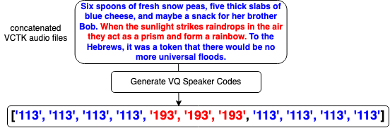
Fig. 2: VQ speaker codes are generated at each sliding window, for a given audio file that contains two different speakers. The codes determine which regions of speech belong to speaker A (113) versus speaker B (193).

6 Speaker Diarization Task

The goal of speaker diarization is to annotate which regions of speech belong to different speakers. We simulated a simple diarization task by concatenating audio files from speakers in our VCTK test conditions, so that there were 2 speakers and 3 turns per audio file, as shown in Figure 2. We used a 2s sliding window (250ms overlap) to obtain short segments of audio. For our VQ-based methods, a speaker code was obtained for each segment. Single-speaker audio VQ reference codes were used as a guide as well as knowledge that 2 speakers were present in each file. For example, if the speaker code 113 for an audio segment belonged to speaker A, then we labeled that region as speaker A. In all systems, sometimes two different speakers were mapped into the same VQ code during training. In the case where speaker could not be determined, we chose speaker A or speaker B randomly. We compared our predictions with the Track1 x-vector baseline from the 2019 DIHARD challenge. It used PLDA scoring and agglomerative hierarchical clustering [17]. Diarization clustering for the baseline method was tuned on the DIHARD dev set, and evaluated on each of our VCTK test conditions using knowledge of 2 speakers per audio file. We report diarization error rate (DER) in Table 2. The DER score measures the proportion of time in an audio file wherein: non-speech is incorrectly labeled as speech (false alarm), a speech region is incorrectly labeled as non-speech (miss), and an incorrect speaker label is generated (error). The +Speaker label and +Adversarial loss systems performed better than the strong x-vector baseline on average. The self-supervised system (+Global VQ) did not learn a diverse VQ space, and we observed the same code was generated for all speakers (sometimes referred to as ”codebook collapse”).

Table 2: Speaker diarization error (DER) scores on concatenated VCTK audio. (S: softmax, AS: angular-softmax).

		Condition
Method		C1	C2	C3	C4	Avg
x-vector		24.3	44.6	27.4	46.7	35.8
VQ-VAE		–	–	–	–	–
+ Global VQ		44.4	39.1	44.7	39.6	42.0
+ Speaker label	S	32.4	32.2	31.0	33.1	32.2
	AS	34.6	35.9	36.4	35.9	35.7
+ Adversarial loss	S	32.2	32.3	30.5	32.9	31.9
	AS	37.2	35.6	36.1	35.2	36.0

7 Phone Recognition Task

We conducted a phone recognition task using TIMIT data and a simple LSTM encoder-decoder architecture. The encoder input was either a string of discrete sub-phone VQ codes, or audio features, and the output was a string of the recognized phones. We used the ESPNet[18] Kaldi recipe for CMU AN4 ASR [19] and a single-layer LSTM model with 64 units, trained to 100 epochs, selected the best model based on CTC loss without attention ($mtlalpha=1.0$), and decoded with beam size 20. In TIMIT there were 63 unique phone types. For our VQ methods, first we applied our fine-tuned models to extract VQ code sequences for each audio file. The lengths of sub-phone VQ code sequences depend on the waveform downsampling factor (DSF) from the VQ-VAE encoder (we used DSF$=64$). Likewise, the sub-phone codewords varied by system since each version learned a slightly different VQ sub-phone space. Table 3 shows the number of unique codewords utilized in each system, as well as the mean phone error rate (PER) averaged across all speakers for phone substitution, insertion, deletion, and overall (Sub, Ins, Del, Total). The VQ-VAE systems offer error reductions for insertion and deletion, compared to the strong audio baseline which has fewer substitutions overall. The + Speaker label AS system had better overall performance over the +Global VQ system. These results show it is possible to add global-level speaker components to VQ-VAE without sacrificing quality of sub-phone representations.

Table 3: Phone error rate (% PER) on TIMIT from sub-phone VQ codes or audio. (S: softmax, AS: angular-softmax).

		# VQ	% PER
Method		Codes	Sub	Ins	Del	Total
Audio Baseline		–	13.8	9.4	7.4	30.6
VQ-VAE		140	26.6	8.3	6.0	40.9
+ Global VQ		119	28.0	7.7	6.4	42.1
+ Speaker label	S	139	28.1	9.6	5.8	43.4
	AS	138	27.6	8.0	6.3	41.9
+ Adversarial loss	S	176	28.0	8.6	6.5	43.1
	AS	154	30.4	9.6	6.5	46.5

8 Discussion

We have presented an approach toward learning disentangled representations of global speaker characteristics and sub-phone content that are also useful for downstream tasks. Adding a semi-supervised VQ component with either speaker labels or adversarial loss improves objective estimates of speech synthesis quality, intelligibility, and speaker similarity from the original VQ-VAE in unseen conditions. Additional work on automated MOS scoring research should consider incorporating natural speech as a reference. Our simulated speaker diarization task shows that speaker VQ codes could be adapted for speaker diarization. From our phone recognition experiments, we found that none of the systems utilized the full VQ space (512 codebooks) so future experiments should determine the optimal codebook sizes, which may depend on the language and diversity of speakers. We plan to explore additional disentanglement by including an F0 modeling component. Speaker VQ codes can also be used conveniently for voice conversion, as this would not require external representations (such as x-vector or LDE). Synthesizing speech from discrete VQ codes may facilitate the ability to control expressiveness in text-to-speech synthesis. For example, a particular sequence of VQ codes could be used to control prosody alongside other signal factors.

References

- [1] David Snyder, Daniel Garcia-Romero, Gregory Sell, Daniel Povey, and Sanjeev Khudanpur, “X-vectors: Robust DNN Embeddings for Speaker Recognition,” in 2018 IEEE International Conference on Acoustics, Speech and Signal Processing (ICASSP). IEEE, 2018, pp. 5329–5333.
- [2] Najim Dehak, Patrick J Kenny, Réda Dehak, Pierre Dumouchel, and Pierre Ouellet, “Front-end Factor Analysis for Speaker Verification,” IEEE Transactions on Audio, Speech, and Language Processing, vol. 19, no. 4, pp. 788–798, 2010.
- [3] Weicheng Cai, Jinkun Chen, and Ming Li, “Exploring the Encoding Layer and Loss Function in End-to-End Speaker and Language Recognition System,” in Proc. Odyssey 2018 The Speaker and Language Recognition Workshop, 2018, pp. 74–81.
- [4] Erica Cooper, Cheng-I Lai, Yusuke Yasuda, Fuming Fang, Xin Wang, Nanxin Chen, and Junichi Yamagishi, “Zero-shot Multi-Speaker Text-to-Speech with State-of-the-art Neural Speaker Embeddings,” in ICASSP 2020-2020 IEEE International Conference on Acoustics, Speech and Signal Processing (ICASSP). IEEE, 2020, pp. 6184–6188.
- [5] Shaojin Ding and Ricardo Gutierrez-Osuna, “Group Latent Embedding for Vector Quantized Variational Autoencoder in Non-Parallel Voice Conversion,” Proc. Interspeech 2019, pp. 724–728, 2019.
- [6] Jennifer Williams and Simon King, “Disentangling Style Factors from Speaker Representations,” Proc. Interspeech 2019, pp. 3945–3949, 2019.
- [7] Desh Raj, David Snyder, Daniel Povey, and Sanjeev Khudanpur, “Probing the Information Encoded in X-Vectors,” in 2019 IEEE Automatic Speech Recognition and Understanding Workshop (ASRU). IEEE, 2019, pp. 726–733.
- [8] Raghuveer Peri, Haoqi Li, Krishna Somandepalli, Arindam Jati, and Shrikanth Narayanan, “An Empirical Analysis of Information Encoded in Disentangled Neural Speaker Representations,” in Proc. Odyssey 2020 The Speaker and Language Recognition Workshop, 2020, pp. 194–201.
- [9] Aaron Van Den Oord, Oriol Vinyals, et al., “Neural Discrete Representation Learning,” in Advances in Neural Information Processing Systems, 2017, pp. 6306–6315.
- [10] Janek Ebbers, Michael Kuhlmann, and Reinhold Haeb-Umbach, “Adversarial Contrastive Predictive Coding for Unsupervised Learning of Disentangled Representations,” arXiv preprint arXiv:2005.12963, 2020.
- [11] Yi Zhao, Haoyu Li, Cheng-I Lai, Jennifer Williams, Erica Cooper, and Junichi Yamagishi, “Improved Prosody from Learned F0 Codebook Representations for VQ-VAE Speech Waveform Reconstruction,” Proc. Interspeech, 2020.
- [12] Yaroslav Ganin, Evgeniya Ustinova, Hana Ajakan, Pascal Germain, Hugo Larochelle, François Laviolette, Mario Marchand, and Victor Lempitsky, “Domain-Adversarial Training of Neural Networks,” The Journal of Machine Learning Research, vol. 17, no. 1, pp. 2096–2030, 2016.
- [13] Junichi Yamagishi, Christophe Veaux, and Kirsten MacDonald, “CSTR VCTK Corpus: English Multi-speaker Corpus for CSTR Voice Cloning Toolkit (version 0.92),” 2019.
- [14] John S Garofolo, Lori F Lamel, William M Fisher, Jonathan G Fiscus, and David S Pallett, “DARPA TIMIT Acoustic-Phonetic Continous Speech Corpus CD-ROM. NIST Speech Disc 1-1.1,” STIN, vol. 93, pp. 27403, 1993.
- [15] Jennifer Williams, Joanna Rownicka, Pilar Oplustil, and Simon King, “Comparison of Speech Representations for Automatic Quality Estimation in Multi-Speaker Text-to-Speech Synthesis,” in Proc. Odyssey 2020 The Speaker and Language Recognition Workshop, 2020, pp. 222–229.
- [16] Andrew Cameron Morris, Viktoria Maier, and Phil Green, “From WER and RIL to MER and WIL: Improved Evaluation Measures for Connected Speech Recognition,” in Eighth International Conference on Spoken Language Processing, 2004.
- [17] Gregory Sell, David Snyder, Alan McCree, Daniel Garcia-Romero, Jesús Villalba, Matthew Maciejewski, Vimal Manohar, Najim Dehak, Daniel Povey, Shinji Watanabe, et al., “Diarization is Hard: Some Experiences and Lessons Learned for the JHU Team in the Inaugural DIHARD Challenge,” Proc. Interspeech 2018, pp. 2808–2812, 2018.
- [18] Hirofumi Inaguma et al., “ESPnet-ST: All-in-One Speech Translation Toolkit,” in Proc. of the 58th Annual Meeting of the Association for Computational Linguistics: System Demonstrations. July 2020, pp. 302–311, Association for Computational Linguistics.
- [19] Suyoun Kim, Takaaki Hori, and Shinji Watanabe, “Joint CTC-Attention Based End-to-End Speech Recognition using Multi-Task learning,” CoRR, vol. abs/1609.06773, 2016.