MINVO Basis: Finding Simplexes with Minimum Volume Enclosing Polynomial Curves

Abstract

This paper studies the polynomial basis that generates the smallest $n$-simplex enclosing a given $n^{\text{th}}$-degree polynomial curve in $\mathbb{R}^{n}$. Although the Bernstein and B-Spline polynomial bases provide feasible solutions to this problem, the simplexes obtained by these bases are not the smallest possible, which leads to overly conservative results in many CAD (computer-aided design) applications. We first prove that the polynomial basis that solves this problem (MINVO basis) also solves for the $n^{\text{th}}$-degree polynomial curve with largest convex hull enclosed in a given $n$-simplex. Then, we present a formulation that is independent of the $n$-simplex or $n^{\text{th}}$-degree polynomial curve given. By using Sum-Of-Squares (SOS) programming, branch and bound, and moment relaxations, we obtain high-quality feasible solutions for any $n\in\mathbb{N}$, and prove (numerical) global optimality for $n=1,2,3$ and (numerical) local optimality for $n=4$. The results obtained for $n=3$ show that, for any given $3^{\text{rd}}$-degree polynomial curve in $\mathbb{R}^{3}$, the MINVO basis is able to obtain an enclosing simplex whose volume is $2.36$ and $254.9$ times smaller than the ones obtained by the Bernstein and B-Spline bases, respectively. When $n=7$, these ratios increase to $902.7$ and $2.997\cdot 10^{21}$, respectively.

Video: https://youtu.be/TXR8mXCaMNg
Code: https://github.com/mit-acl/minvo

1 Introduction

Polyhedral enclosures of a given polynomial curve have a crucial role in a large number of CAD algorithms to compute curve intersections, perform ray tracing, or obtain minimum distances between convex shapes [1, 2, 3, 4, 5]. These polyhedral enclosures are also used in rasterization [6, 7], mesh generation [8], path planning for numerical control machines [9, 10], and trajectory optimization for robots [11, 12, 13, 14, 15]. Many of these works leverage the convex hull property of the Bernstein basis (polynomial basis used by Bézier curves) to obtain these polyhedral enclosures, although some works use the B-Spline basis instead [16, 17].

Although both the Bernstein basis and B-Spline basis have many useful properties, they are not designed to generate the smallest $n$-simplex that encloses a given $n^{\text{th}}$-degree polynomial curve in $\mathbb{R}^{n}$. This directly translates into undesirably conservative results in many of the aforementioned applications. Polyhedral enclosures with more than $n+1$ vertices (i.e., not simplexes) can provide tighter volume approximations, but at the expense of a larger number of vertices, which can eventually increase the computation time in real-time applications. The main focus of this paper is therefore on simplex enclosures.

Moreover, and rather than designing an iterative algorithm that needs to be run for each different curve to obtain the smallest simplex enclosure, this paper studies a novel polynomial basis that is designed by construction to minimize the volume of this simplex. Compared to an iterative algorithm, this basis benefits from the properties of linearity (the simplex is a linear transformation of the coefficient matrix of the curve, avoiding therefore the need of expensive iterative algorithms) and independence with respect to the curve (the matrix that defines this linear transformation is the same one for all the curves of the same degree). These two properties are highly desirable in real-time computing and/or when used in an optimization problem.

In summary, this paper studies the polynomial basis that generates the $n$-simplex with minimum volume enclosing a given $n^{\text{th}}$-degree polynomial curve. Additionally, we also investigate the related problem of obtaining the $n^{\text{th}}$-degree polynomial curve with largest convex hull enclosed in a given $n$-simplex. The contributions of this paper are summarized as follows:

• Formulation of the optimization problem whose minimizer is the polynomial basis that generates the smallest $n$-simplex that encloses any given $n^{\text{th}}$-degree polynomial curve. We show that this basis also obtains the $n^{\text{th}}$-degree polynomial curve with largest convex hull enclosed in any given $n$-simplex. Another formulation that imposes a specific structure on the polynomials of the basis is also presented.

• We derive high-quality feasible solutions for any $n\in\mathbb{N}$, obtaining simplexes that, for $n=3$, are $2.36$ and $254.9$ times smaller than the ones obtained using the Bernstein and B-Spline bases respectively. For $n=7$, these values increase to 902.7 and $2.997\cdot 10^{21}$, respectively.

• Numerical global optimality (with respect to the volume) is proven for $n=1,2,3$ using SOS, branch and bound, and moment relaxations. Numerical local optimality is proven for $n=4$, and feasibility is guaranteed for $n\geq 5$.

• Extension to polynomial curves embedded in subspaces of higher dimensions, and to some rational curves.

2 Related work

Herron [18] attempted to find (for $n=2$ and $n=3$) the smallest $n$-simplex enclosing an $n^{\text{th}}$-degree polynomial curve. The approach of [18] imposed a specific structure on the polynomials of the basis and then solved the associated nonconvex optimization problem over the roots of those polynomials. For this specific structure of the polynomials, a global minimizer was found for $n=2$, and a local minimizer was found for $n=3$. However, global optimality over all possible polynomials was not proven, and only the cases $n=2$ and $n=3$ were studied. Similarly, in the results of [19], Kuti et al. use the algorithm proposed in [20] to obtain a minimal 2-simplex that encloses a specific $2^{\text{nd}}$-degree polynomial curve. However, this approach requires running the algorithm for each different curve, no global optimality is shown, and only one case with $n=2$ was analyzed. There are also works that have derived bounds on the distance between the control polygon and the curve [21, 22, 23], while others propose the SLEFE (subdividable linear efficient function enclosure) to enclose spline curves via subdivision [24, 25, 26, 27]. However, the SLEFE depends pseudo-linearly on the coefficients of the polynomial curve (i.e., linearly except for a min/max operation) [24], which is disadvantageous when the curve is a decision variable in a time-critical optimization problem. This paper focuses instead on enclosures that depend linearly on the coefficients of the curve.

Other works have focused on the properties of the smallest $n$-simplex that encloses a given generic convex body. For example, [28, 29] derived some bounds for the volume of this simplex, while Klee [30] showed that any locally optimal simplex (with respect to its volume) that encloses a convex body must be a centroidal simplex. In other words, the centroid of its facets must belong to the convex body. Applied to a curve $P$, this means that the centroid of its facets must belong to $\text{conv}\left(P\right)$. Although this is a necessary condition, it is not sufficient for local optimality.

When the convex body is a polyhedron (or equivalently the convex hull of a finite set of points), [31] classifies the possible minimal circumscribing simplexes, and this classification is later used by [32] to derive a $O(k^{4})$ algorithm that computes the smallest simplex enclosing a finite set of $k$ points. This problem is also crucial for the hyperspectral unmixing in remote sensing, to be able to find the proportions or abundances of each macroscopic material (endmember) contained in a given image pixel [33, 34], and many different iterative algorithms have been proposed towards this end [35, 36, 37]. All these works focus on obtaining the enclosing simplex for a generic discrete set of points. Our work focuses instead on polynomial curves and, by leveraging their structure, we can avoid the need to iterate and/or discretize the curve.

The convex hull of curves has also been studied in the literature. For instance, [38, 39, 40] studied the boundaries of these convex hulls, while [41] focused on the patches of the convex hull of trajectories of polynomial dynamical systems. For a moment curve $\left[\begin{array}[]{cccc}t&t^{2}&\cdots&t^{n}\end{array}\right]^{T}$ (where $t$ is in some interval $[a,b]$), [42] found that the number of points needed to represent every point in the convex hull of this curve is $\frac{n+1}{2}$, giving therefore a tighter bound than the $n+1$ points found using the Carathéodory’s Theorem [43, 44]. This particular curve and the volume of its convex hull were also analyzed by [45] in the context of moment spaces and orthogonal polynomials. Although many useful properties of the convex hull of a curve are shown in all these previous works, none of them addresses the problem of finding the polynomial curve with largest convex hull enclosed in a given simplex.

3 Preliminaries

3.1 Notation and Definitions

The notation used throughout the paper is summarized in Table 1. Unless otherwise noted, all the indexes in this paper start at $0$. For instance, $\boldsymbol{M}_{0,3}$ is the fourth element of the first row of the matrix $\boldsymbol{M}$. Let us also introduce the two following common definitions and their respective notations:

Polynomial curve $P$ of degree $n$ and dimension $k$: $$P:=\left\{\boldsymbol{p}(t)\;|\;t\in[a,b],a\in\mathbb{R},b\in\mathbb{R},b>a\right\}$$ where $\boldsymbol{p}(t):=\left[\begin{array}[]{ccc}p_{0}(t)&\cdots&p_{k-1}(t)\end{array}\right]^{T}:=\boldsymbol{P}\boldsymbol{t}\in\mathbb{R}^{k}$, $p_{i}(t)$ is a polynomial in $\mathbb{R}[t]$, and $n\in\mathbb{N}$ is the highest degree of all the $p_{i}(t)$. The $k\times(n+1)$ matrix $\boldsymbol{P}$ is the coefficient matrix. Without loss of generality we will use the interval $t\in[-1,1]$ (i.e., $a=-1$ and $b=1$), and assume that the parametrization of $\boldsymbol{p}(t)$ has minimal degree (i.e., no other polynomial parametrization with lower degree produces the same spatial curve $P$). The subspace containing $P$ and that has the smallest dimension will be denoted as $\mathcal{M}\subseteq\mathbb{R}^{k}$, and its dimension will be $m$. We will work with the case $n=m=k$, and refer to such curves simply as $n^{\text{th}}$-degree polynomial curves. Note that we will use the term polynomial curve to refer to a curve with only one segment, and not to a curve with several polynomial segments. The set of all possible $n^{\text{th}}$-degree polynomial curves will be denoted as $\mathcal{P}^{n}$. Section 7 will then extend the results to curves with arbitrary $n$, $m$ and $k$.

Table 1: Notation used in this paper.

Symbol	Meaning
$a$, $\boldsymbol{a}$, $\boldsymbol{A}$	Scalar, column vector, matrix
$|\boldsymbol{A}|$, $\text{tr}(\boldsymbol{A})$	Determinant of $\boldsymbol{A}$, trace of $\boldsymbol{A}$
$\boldsymbol{t}$	$\left[\begin{array}[]{ccc}t^{r}&t^{r-1}\cdots&1\end{array}\right]^{T}$ ($r$ given by the context)
$\hat{\boldsymbol{t}}$	$\left[\begin{array}[]{cccc}1&\cdots&t^{r-1}&t^{r}\end{array}\right]^{T}$ ($r$ given by the context)
$\mathbb{R}[t]$	Set of univariate polynomials in $t$ with coefficients in $\mathbb{R}$
$\boldsymbol{p}(t)$	Column vector whose coordinates are polynomials in $\mathbb{R}[t]$
$P$	Polynomial curve $P:=\left\{\boldsymbol{p}(t)\;|\;t\in[-1,1]\right\}$
$\boldsymbol{P}$	Coefficient matrix of $P$. $\boldsymbol{p}(t)=\boldsymbol{P}\boldsymbol{t}$
$\mathcal{P}^{n}$	Set of all possible $n^{\text{th}}$-degree polynomial curves
$\text{conv}(P)$	Convex hull of $P$
$n$	Maximum degree of the entries of $\boldsymbol{p}(t)$
$k$	Number of rows of $\boldsymbol{p}(t)$
$\mathcal{M}$	Subspace with the smallest dimension that contains $P$. $\mathcal{M}\subseteq\mathbb{R}^{k}$
$m$	Dimension of $\mathcal{M}$
$S$	Simplex
$\mathcal{S}^{n}$	Set of all possible $n$-simplexes
$\boldsymbol{V}$	Matrix whose columns are the vertices of a simplex. This definition will be generalized in Section 7.1
$\boldsymbol{0}$, $\boldsymbol{1}$	Column vectors of zeros and ones
$\boldsymbol{a}\geq\boldsymbol{b}$	Element-wise inequality
$s$	Number of intervals the polynomial curve is subdivided into ($s=1$ means no subdivision)
SL$h$	SLEFE of a polynomial curve using $h$ breakpoints in each interval of subdivision
$\propto$	Proportional to
$\partial\;\cdot$	Frontier of a set
$\left\lfloor\cdot\right\rfloor$	Floor function
$\text{abs}(\cdot)$	Absolute value
$\cdot_{a\times b}$	Size of a matrix ($a$ rows $\times$ $b$ columns)
$\boldsymbol{e}$	$\left[\begin{array}[]{ccccc}0&0&\cdots&0&1\end{array}\right]^{T}$ (size given by the context)
$\boldsymbol{I}_{n}$	Identity matrix of size $n\times n$
$\boldsymbol{M}_{:,c:d}$	Matrix formed by columns $c,c+1,\ldots,d$ of $\boldsymbol{M}$
$\mathbb{S}_{+}^{a}$	Positive semidefinite cone (set of all symmetric positive semidefinite $a\times a$ matrices)
$\text{vol}(\cdot)$	Volume (Lebesgue measure)
$\boldsymbol{\pi}$	Hyperplane
$\text{dist}(\boldsymbol{a},\boldsymbol{\pi})$	Distance between the point $\boldsymbol{a}$ and the hyperplane $\boldsymbol{\pi}$
$\text{odd}(a,b)$	1 if both $a$ and $b$ are odd, 0 otherwise
NLO, NGO	Numerical Local Optimality, Numerical Global Optimality
$\text{MV},\text{Be},\text{BS}$	MINVO, Bernstein, and B-Spline
	Color notation for the MV, Be, and BS bases respectively

$n$-simplex: Convex hull of $n+1$ affinely independent points $\boldsymbol{v}_{0},\ldots,\boldsymbol{v}_{n}\in\mathbb{R}^{n}$. These points are the vertices of the simplex, and will be stacked in the matrix of vertices $\boldsymbol{V}:=\left[\begin{array}[]{ccc}\boldsymbol{v}_{0}&\cdots&\boldsymbol{v}_{n}\end{array}\right]$. The letter $S$ will denote a particular simplex, while $\mathcal{S}^{n}$ will denote the set of all possible $n$-simplexes. A simplex with $\boldsymbol{V}=\left[\begin{array}[]{cc}\boldsymbol{0}&\boldsymbol{I}_{n}\end{array}\right]$ will be called the standard $n$-simplex.

We will use the basis matrix of a segment of a non-clamped uniform B-Spline for comparison [46, 47, 48], and refer to this basis simply as the B-Spline basis.

Moreover, throughout this paper we will use the term numerical local optimality (NLO) to classify a solution for which the first-order optimality measure and the maximum constraint violation are smaller than a predefined small tolerance [49]. Similarly, we will use the term numerical global optimality (NGO) to classify a feasible solution for which the difference between its objective value and a lower bound on the global minimum (typically obtained via a relaxation of the problem) is less than a specific small tolerance. All the tolerances and parameters of the numerical solvers used are available in the attached code.

Finally, and for purposes of clarity, we will use the term MINVO basis to refer to both the global minimizers of the problem (proved for $n=1,2,3$) and the proposed locally-optimal/feasible solutions (obtained for $n\geq 4$).

3.2 Volume of the Convex Hull of a Polynomial Curve

At several points throughout the paper, we will make use of the following theorem, that we prove in A:

Theorem 1: The volume of the convex hull of $P\in\mathcal{P}^{n}$ ($t\in[-1,1]$), is given by: $$\text{vol}\left(\text{conv}\left(P\right)\right)=\frac{\text{abs}\left(\left|\boldsymbol{P}_{:,0:n-1}\right|\right)}{n!}2^{\frac{n(n+1)}{2}}\prod_{0\leq i<j\leq n}\left(\frac{j-i}{j+i}\right)$$ Proof: See A. $\square$

Note that, as the curve $P$ satisfies $n=m=k$ (see Section 3.1), the volume of its convex hull is nonzero and therefore $\left|\boldsymbol{P}_{:,0:n-1}\right|\neq 0$.

4 Problems definition

As explained in Section 1, the goal of this paper is to find the smallest simplex $S\in\mathcal{S}^{n}$ enclosing a given polynomial curve $P\in\mathcal{P}^{n}$, and to find the polynomial curve $P\in\mathcal{P}^{n}$ with largest convex hull enclosed in a given simplex $S\in\mathcal{S}^{n}$.

4.1 Given $P\in\mathcal{P}^{n}$, find $S\in\mathcal{S}^{n}$

Problem 1: Given the polynomial curve $P\in\mathcal{P}^{n}$, find the simplex $S\in\mathcal{S}^{n}$ with minimum volume that contains $P$. In other words: $$\min_{S\in\mathcal{S}^{n}}\quad\text{vol}(S)$$ $$\begin{array}[]{cc}\text{s.t.}&P\subset S\end{array}$$

For $n=2$, Problem 1 tries to find the triangle with the smallest area that contains a planar $2^{\text{nd}}$-degree polynomial curve. For $n=3$, it tries to find the tetrahedron with the smallest volume that contains a $3^{\text{rd}}$-degree polynomial curve in 3D. Similar geometric interpretations apply for higher $n$.

Letting $f_{1}$ denote the objective function of this problem, we have that $f_{1}:=\text{vol}(S)\propto\text{abs}\left(\left|\left[\begin{array}[]{cc}\boldsymbol{V}^{T}&\boldsymbol{1}\end{array}\right]\right|\right)$. Note that, as the volume of the convex hull of $P$ is nonzero (see Section 3.2), then it is guaranteed that $\left|\left[\begin{array}[]{cc}\boldsymbol{V}^{T}&\boldsymbol{1}\end{array}\right]\right|\neq 0$.

4.2 Given $S\in\mathcal{S}^{n}$, find $P\in\mathcal{P}^{n}$

Problem 2: Given a simplex $S\in\mathcal{S}^{n}$, find the polynomial curve $P\in\mathcal{P}^{n}$ contained in $S$, whose convex hull has maximum volume: $$\min_{P\in\mathcal{P}^{n}}\quad-\text{vol}(\text{conv}(P))$$ $$\begin{array}[]{cc}\text{s.t.}&P\subset S\end{array}$$

By the definition of a simplex (see Section 3.1), its vertices are affinely independent and therefore the matrix of vertices of the given simplex $S$ satisfies $\left|\left[\begin{array}[]{cc}\boldsymbol{V}^{T}&\boldsymbol{1}\end{array}\right]\right|\neq 0$.

Letting $f_{2}$ denote the objective function of this problem, we have that $f_{2}:=-\text{vol}(\text{conv}(P))\propto-\text{abs}\left(\left|\boldsymbol{P}_{:,0:n-1}\right|\right)$. Now note that the optimal solution for this problem is guaranteed to satisfy $\left|\boldsymbol{P}_{:,0:n-1}\right|\neq 0$, which can be easily proven by noting that we are maximizing the absolute value of $\left|\boldsymbol{P}_{:,0:n-1}\right|$, and that there exists at least one feasible solution (for example the Bézier curve whose control points are the vertices of $S$) with $\left|\boldsymbol{P}_{:,0:n-1}\right|\neq 0$.

5 Equivalent Formulation

Let us now study the constraints and the objective functions of Problems 1 and 2.

5.1 Constraints of Problems 1 and 2

Both problems share the same constraint $P\subset S$ (i.e., $\boldsymbol{p}(t)\in S\;\;\forall t\in[-1,1]$), which is equivalent to $\boldsymbol{p}(t)$ being a convex combination of the vertices $\boldsymbol{v}_{i}$ of the simplex for $t\in[-1,1]$:

$$P\subset S\equiv\left\{\begin{aligned} &\boldsymbol{p}(t)=\textstyle\sum_{i=0}^{n}\lambda_{i}(t)\boldsymbol{v}_{i}\\ &\textstyle\sum_{i=0}^{n}\lambda_{i}(t)=1\quad\forall t\\ &\lambda_{i}(t)\geq 0\quad\forall i=0,\dots,n\;\;\forall t\in[-1,1]\end{aligned}\right.$$ (1)

The variables $\lambda_{i}(t)$ are usually called barycentric coordinates [50, 51, 52], and their geometric interpretation is as follows. Let us first define $\boldsymbol{\pi}_{i}$ as the hyperplane that passes through the points $\{\boldsymbol{v}_{0},\boldsymbol{v}_{1},\ldots,\boldsymbol{v}_{n}\}\backslash\{\boldsymbol{v}_{i}\}$, and $\boldsymbol{n}_{i}$ as its normal vector that points towards the interior of the simplex. Choosing now $q\in\{0,\ldots,n\}\backslash\{i\}$, and using the fact that $\sum_{j=0}^{n}\lambda_{j}(t)=1$, we have that $\boldsymbol{p}(t)=\boldsymbol{v}_{q}+\sum_{j=0}^{n}\lambda_{j}(t)\left(\boldsymbol{v}_{j}-\boldsymbol{v}_{q}\right)$.

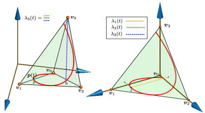
Figure 1: Geometric interpretation of $\lambda_{i}(t)$. Each $\lambda_{i}(t)$ represents the distance between the curve $\boldsymbol{p}(t)$ and the hyperplane formed by the vertices $\{\boldsymbol{v}_{0},\boldsymbol{v}_{1},\ldots,\boldsymbol{v}_{n}\}\backslash\{\boldsymbol{v}_{i}\}$, divided by the distance from the vertex $\boldsymbol{v}_{i}$ to that hyperplane (left). For the standard $3$-simplex in 3D (i.e., $\boldsymbol{V}=\left[\begin{array}[]{cc}\boldsymbol{0}&\boldsymbol{I}_{3}\end{array}\right]$), the curve in red has $\boldsymbol{p}(t)=\left[\begin{array}[]{ccc}\lambda_{1}(t)&\lambda_{2}(t)&\lambda_{3}(t)\end{array}\right]^{T}$ (right).

Therefore:

$$\text{dist}\left(\boldsymbol{p}(t),\boldsymbol{\pi}_{i}\right):=\left(\boldsymbol{p}(t)-\boldsymbol{v}_{q}\right)^{T}\boldsymbol{n}_{i}=\displaystyle\sum_{j=0}^{n}\lambda_{j}(t)\left(\boldsymbol{v}_{j}-\boldsymbol{v}_{q}\right)^{T}\boldsymbol{n}_{i}=$$

$$=\lambda_{i}(t)\left(\boldsymbol{v}_{i}-\boldsymbol{v}_{q}\right)^{T}\boldsymbol{n}_{i}=\lambda_{i}(t)\;\text{dist}\left(\boldsymbol{v}_{i},\boldsymbol{\pi}_{i}\right)\,,$$

which implies that

$$\lambda_{i}(t)=\frac{\text{dist}\left(\boldsymbol{p}(t),\boldsymbol{\pi}_{i}\right)}{\text{dist}\left(\boldsymbol{v}_{i},\boldsymbol{\pi}_{i}\right)}\,.$$ (2)

Hence, $\lambda_{i}(t)$ represents the ratio between the distance from the point $\boldsymbol{p}(t)$ of the curve to the hyperplane $\boldsymbol{\pi}_{i}$ and the distance from $\boldsymbol{v}_{i}$ to that hyperplane $\boldsymbol{\pi}_{i}$ (see Figure 1 for the case $n=3$). From Eq. 2 it is clear that each $\lambda_{i}(t)$ is an $n^{\text{th}}$-degree polynomial, that we will write as $\lambda_{i}(t):=\boldsymbol{\lambda}_{i}^{T}\boldsymbol{t}$, where $\boldsymbol{\lambda}_{i}$ is its vector of coefficients. Matching now the coefficients of $\boldsymbol{p}(t)$ with the ones of $\sum_{i=0}^{n}\lambda_{i}(t)\boldsymbol{v}_{i}$, the first constraint of Eq. 1 can be rewritten as $\boldsymbol{P}=\boldsymbol{V}\boldsymbol{A}$, where

$$\boldsymbol{A}:=\left[\begin{array}[]{c}\boldsymbol{\lambda}_{0}^{T}\\ \boldsymbol{\lambda}_{1}^{T}\\ \vdots\\ \boldsymbol{\lambda}_{n}^{T}\end{array}\right]=\left[\begin{array}[]{llll}\boldsymbol{\lambda}_{0}&\boldsymbol{\lambda}_{1}&\cdots&\boldsymbol{\lambda}_{n}\end{array}\right]^{T}\,.$$

Note that $\boldsymbol{A}$ is a $(n+1)\times(n+1)$ matrix whose $i^{\text{th}}$ row contains the coefficients of the polynomial $\lambda_{i}(t)$ in decreasing order. The second and third constraints of Eq. 1 can be rewritten as $\boldsymbol{A}^{T}\boldsymbol{1}=\boldsymbol{e}$ and $\boldsymbol{A}\boldsymbol{t}\geq 0\;\forall t\in[-1,1]$ respectively. We conclude therefore that

$$P\subset S\equiv\left\{\begin{aligned} &\boldsymbol{P}=\boldsymbol{V}\boldsymbol{A}\\ &\boldsymbol{A}^{T}\boldsymbol{1}=\boldsymbol{e}\\ &\boldsymbol{A}\boldsymbol{t}\geq 0\;\;\forall t\in[-1,1]\end{aligned}\right.$$ (3)

5.2 Objective Function of Problem 1

Using the constraints in Eq. 3, and noting that the matrix $\boldsymbol{A}$ is invertible (as proven in B), we can write

$$f_{1}\propto\text{abs}\left(\left|\left[\begin{array}[]{cc}\boldsymbol{V}^{T}&\boldsymbol{1}\end{array}\right]\right|\right)=\text{abs}\left(\left|\boldsymbol{A}^{-T}\left[\begin{array}[]{cc}\boldsymbol{P}^{T}&\boldsymbol{e}\end{array}\right]\right|\right)\propto$$

$$\propto\text{abs}\left(\left|\boldsymbol{A}^{-1}\right|\right)=\frac{1}{\text{abs}\left(\left|\boldsymbol{A}\right|\right)}\,,$$

where we have used the fact that everything inside $\left[\begin{array}[]{cc}\boldsymbol{P}^{T}&\boldsymbol{e}\end{array}\right]$ is given (i.e., not a decision variable of the optimization problem), and the fact that $\left|\boldsymbol{A}\right|=|\boldsymbol{A}^{T}|$. We can therefore minimize $-\text{abs}\left(\left|\boldsymbol{A}\right|\right)$. Note that now the objective function $f_{1}$ is independent of the given curve $P$.

5.3 Objective Function of Problem 2

Similar to the previous subsection, and noting that $\boldsymbol{V}$ is given in Problem 2, we have that

$$f_{2}\propto-\text{abs}\left(\left|\boldsymbol{P}_{:,0:n-1}\right|\right)=-\text{abs}\left(\left|\left[\begin{array}[]{c}\boldsymbol{P}\\ \boldsymbol{e}^{T}\end{array}\right]\right|\right)=$$

$$=-\text{abs}\left(\left|\left[\begin{array}[]{c}\boldsymbol{V}\\ \boldsymbol{1}^{T}\end{array}\right]\boldsymbol{A}\right|\right)\propto-\text{abs}\left(\left|\boldsymbol{A}\right|\right)\,,$$

and therefore the objective function $f_{2}$ is now independent of the given simplex $S$.

5.4 Equivalent Formulation for Problems 1 and 2

Note that now the dependence on the given polynomial curve (for Problem 1) or on the given simplex (for Problem 2) appears only in the constraint $\boldsymbol{P}=\boldsymbol{V}\boldsymbol{A}$. As $\boldsymbol{A}$ is invertible (see B), we can safely remove this constraint from the optimization, leaving $\boldsymbol{A}$ as the only decision variable, and then use $\boldsymbol{P}=\boldsymbol{V}\boldsymbol{A}$ to obtain $\boldsymbol{V}$ (for Problem 1) or $\boldsymbol{P}$ (for Problem 2). We end up therefore with the following optimization problem:

Problem 3: $$\min_{\boldsymbol{A}\in\mathbb{R}^{(n+1)\times(n+1)}}\quad-\text{abs}\left(\left|\boldsymbol{A}\right|\right)$$ s.t. $\displaystyle\boldsymbol{A}^{T}\boldsymbol{1}=\boldsymbol{e}$ $\displaystyle\boldsymbol{A}\boldsymbol{t}\geq\boldsymbol{0}\quad\forall t\in[-1,1]$

Remark: As detailed above, Problem 3 does not depend on the specific given $n^{\text{th}}$-degree polynomial curve (for Problem 1) or on the specific given $n$-simplex (for Problem 2). Hence, its optimal solution $\boldsymbol{A}^{*}$ for a specific $n$ can be applied to obtain the optimal solution of Problem 1 for any given polynomial curve $P\in\mathcal{P}^{n}$ (by using $\boldsymbol{V}^{*}=\boldsymbol{P}\left(\boldsymbol{A}^{*}\right)^{-1}$) and to obtain the optimal solution of Problem 2 for any given simplex $S\in\mathcal{S}^{n}$ (by using $\boldsymbol{P}^{*}=\boldsymbol{V}\boldsymbol{A}^{*}$).

As the objective function of Problem 3 is the determinant of the nonsymmetric matrix $\boldsymbol{A}$, it is clearly a nonconvex problem. We can rewrite the constraint $\boldsymbol{A}\boldsymbol{t}\geq\boldsymbol{0}\quad\forall t\in[-1,1]$ of Problem 3 using Sum-Of-Squares programming [53]:

• If $n$ is odd, $\lambda_{i}(t)\geq 0\;\;\forall t\in[-1,1]$ if and only if

  $$\left\{\begin{aligned} &\lambda_{i}(t)=\hat{\boldsymbol{t}}^{T}\left((t+1)\boldsymbol{W}_{i}+(1-t)\boldsymbol{V}_{i}\right)\hat{\boldsymbol{t}}\\ &\boldsymbol{W}_{i}\in\mathbb{S}_{+}^{\frac{n+1}{2}},\boldsymbol{V}_{i}\in\mathbb{S}_{+}^{\frac{n+1}{2}}\end{aligned}\right.$$

• If $n$ is even, $\lambda_{i}(t)\geq 0\;\;\forall t\in[-1,1]$ if and only if

  $$\left\{\begin{aligned} &\lambda_{i}(t)=\hat{\boldsymbol{t}}^{T}\boldsymbol{W}_{i}\hat{\boldsymbol{t}}+\hat{\boldsymbol{t}}^{T}(t+1)(1-t)\boldsymbol{V}_{i}\hat{\boldsymbol{t}}\\ &\boldsymbol{W}_{i}\in\mathbb{S}_{+}^{\frac{n}{2}+1},\boldsymbol{V}_{i}\in\mathbb{S}_{+}^{\frac{n}{2}}\end{aligned}\right.$$

Note that the if and only if condition applies because $\lambda_{i}(t)$ is a univariate polynomial [53]. The decisions variables would be the positive semidefinite matrices $\boldsymbol{W}_{i}$ and $\boldsymbol{V}_{i}$, $i=0,\ldots,n$. Another option is to use the Markov–Lukács Theorem ([54, Theorem 1.21.1],[55, Theorem 2.2],[56]):

• If $n$ is odd, $\lambda_{i}(t)\geq 0\;\;\forall t\in[-1,1]$ if and only if

  $$\lambda_{i}(t)=(t+1)g_{i}^{2}(t)+(1-t)h_{i}^{2}(t)\,.$$

• If $n$ is even, $\lambda_{i}(t)\geq 0\;\;\forall t\in[-1,1]$ if and only if

  $$\lambda_{i}(t)=g_{i}^{2}(t)+(t+1)(1-t)h_{i}^{2}(t)\,.$$

where $g_{i}(t)$ and $h_{i}(t)$ are polynomials of degrees $\operatorname{deg}(g_{i}(t))\leq\lfloor n/2\rfloor$ and $\operatorname{deg}(h_{i}(t))\leq\lfloor(n-1)/2\rfloor$. The decision variables would be the coefficients of the polynomials $g_{i}(t)$ and $h_{i}(t)$, $i=0,\ldots,n$. In C we derive the Karush–Kuhn–Tucker (KKT) conditions of Problem 3 using this theorem.

Regardless of the choice of the representation of the constraint $\boldsymbol{A}\boldsymbol{t}\geq\boldsymbol{0}\;\;\forall t\in[-1,1]$ (SOS or the Markov–Lukács Theorem), no generality has been lost so far. However, these formulations easily become intractable for large $n$ due to the high number of decision variables. We can reduce the number of decision variables of Problem 3 by imposing a structure in $\lambda_{i}(t)$. As Problem 1 is trying to minimize the volume of the simplex, we can impose that the facets of the $n$-simplex be tangent to several internal points $\boldsymbol{p}(t)$ of the curve (with $t\in(-1,1)$), and in contact with the first and last points of the curve ($\boldsymbol{p}(-1)$ and $\boldsymbol{p}(1)$) [32, 30]. Using the geometric interpretation of the $\lambda_{i}(t)$ given in Section 5.1, this means that each $\lambda_{i}(t)$ should have either real double roots in $t\in(-1,1)$ (where the curve is tangent to a facet), and/or roots at $t\in\{-1,1\}$. These conditions, together with an additional symmetry condition between different $\lambda_{i}(t)$, translate into the formulation shown in Problem 4, in which the decisions variables are the roots of $\lambda_{i}(t)$ and the coefficients $b_{i}$.

Problem 4: $$\min_{\boldsymbol{A}\in\mathbb{R}^{(n+1)\times(n+1)}}\quad-\text{abs}\left(\left|\boldsymbol{A}\right|\right)\quad\text{subject to:}$$ If $n$ is odd: $\displaystyle\lambda_{i}(t)=-b_{i}(t-1)\textstyle\prod_{j=1}^{\frac{n-1}{2}}(t-t_{ij})^{2}\hskip 5.69046pt$ $\displaystyle i=0,2,\ldots,n-1$ $\displaystyle\lambda_{i}(t)=\lambda_{n-i}(-t)\hskip 85.35826pt$ $\displaystyle i=1,3,\ldots,n$ $\displaystyle b_{i}\geq 0\quad$ $\displaystyle i=0,2,\ldots,n-1$ $\displaystyle\boldsymbol{A}^{T}\boldsymbol{1}=\boldsymbol{e}$ If $n$ is even: $\displaystyle\lambda_{i}(t)=-b_{i}(t+1)(t-1)\textstyle\prod_{j=1}^{\frac{n-2}{2}}(t-t_{ij})^{2}\quad$ $\displaystyle i\text{ odd integer}\in\left[0,n/2-1\right]$ $\displaystyle\lambda_{i}(t)=b_{i}\textstyle\prod_{j=1}^{\frac{n}{2}}(t-t_{ij})^{2}$ $\displaystyle i\text{ even integer}\in\left[0,n/2-1\right]$ $\displaystyle\lambda_{i}(t)=\lambda_{n-i}(-t)$ $\displaystyle i=n/2+1,\ldots,n$ $\displaystyle b_{i}\geq 0\quad$ $\displaystyle i=0,1,\dots,n/2$ $\displaystyle\boldsymbol{A}^{T}\boldsymbol{1}=\boldsymbol{e}$ $\displaystyle\lambda_{i}(t)=-b_{i}(t+1)(t-1)\textstyle\prod_{j=1}^{\frac{n-2}{4}}(t-t_{ij})^{2}(t+t_{ij})^{2}\quad$ $\displaystyle i=n/2,\;i\text{ odd}$ $\displaystyle\lambda_{i}(t)=b_{i}\textstyle\prod_{j=1}^{\frac{n}{4}}(t-t_{ij})^{2}(t+t_{ij})^{2}$ $\displaystyle i=n/2,\;i\text{ even}$

Letting $f_{i}$ denote the objective function of Problem $i$, the relationship between Problems 1, 2, 3 and 4 is given in Figure 2. First note that the constraints and structure imposed on $\lambda_{i}(t)$ in Problem 4 guarantee that they are nonnegative for $t\in[-1,1]$ and that they sum up to 1. Hence the feasible set of Problem 4 is contained in the feasible set of Problem 3, and therefore, $f_{3}^{*}\leq f_{4}^{*}$ holds. The matrix $\boldsymbol{A}$ found in Problem 3 or 4 can be used to find the vertices of the simplex in Problem 1 (by simply using $\boldsymbol{V}=\boldsymbol{P}\left(\boldsymbol{A}\right)^{-1}$, where $\boldsymbol{P}$ is the coefficient matrix of the polynomial curve given), or to find the coefficient matrix of the polynomial curve in Problem 2 (by using $\boldsymbol{P}=\boldsymbol{V}\boldsymbol{A}$, where $\boldsymbol{V}$ contains the vertices of the given simplex).

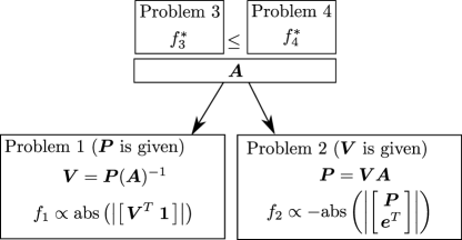
Figure 2: Relationship between Problems 1, 2, 3, and 4: Problem 3 and 4 have the same objective function, but the feasible set of Problem 4 is contained in the feasible set of Problem 3, and therefore $f_{3}^{*}\leq f_{4}^{*}$. Both Problem 3 and 4 generate a solution $\boldsymbol{A}$, which can be applied to any polynomial curve $P\in\mathcal{P}^{n}$ to find the simplex $S\in\mathcal{S}^{n}$ in Problem 1, or to any simplex $S\in\mathcal{S}^{n}$ to find the polynomial curve $P\in\mathcal{P}^{n}$ in Problem 2.

6 Results

6.1 Results for $n=1,2,\dots,7$

Table 2: Roots of each $\lambda_{i}(t)$ of the MINVO basis. $\boldsymbol{r}(\lambda_{i}(t))$ is the column vector that contains the roots of $\lambda_{i}(t)$. All the roots lying in $(-1,1)$ are double roots, while the ones in $\{-1,1\}$ are single roots. Each $\lambda_{i}(t)$ has $n$ real roots in total. These roots are plotted in Figure 9.

$\boldsymbol{n}$	Roots of $\lambda_{i}(t),\;t\in[-1,1]$
$1$	$\left[\begin{array}[]{c}\boldsymbol{r}(\lambda_{0})^{T}\\ \boldsymbol{r}(\lambda_{1})^{T}\end{array}\right]=\left[\begin{array}[]{c}1.0\\ -1.0\end{array}\right]$
$2$	$\left[\begin{array}[]{c}\boldsymbol{r}(\lambda_{0})^{T}\\ \boldsymbol{r}(\lambda_{1})^{T}\\ \boldsymbol{r}(\lambda_{2})^{T}\end{array}\right]=\left[\begin{array}[]{cc}\frac{1}{\sqrt{3}}&\mathrm{}\\ -1.0&1.0\\ -\frac{1}{\sqrt{3}}&\mathrm{}\end{array}\right]$
$3$	$\left[\begin{array}[]{c}\boldsymbol{r}(\lambda_{0})^{T}\\ \boldsymbol{r}(\lambda_{1})^{T}\\ \boldsymbol{r}(\lambda_{2})^{T}\\ \boldsymbol{r}(\lambda_{3})^{T}\end{array}\right]\approx\left[\begin{array}[]{cc}0.03088&1.0\\ -1.0&0.7735\\ -0.7735&1.0\\ -1.0&-0.03088\end{array}\right]$
$4$	$\left[\begin{array}[]{c}\boldsymbol{r}(\lambda_{0})^{T}\\ \boldsymbol{r}(\lambda_{1})^{T}\\ \boldsymbol{r}(\lambda_{2})^{T}\\ \boldsymbol{r}(\lambda_{3})^{T}\\ \boldsymbol{r}(\lambda_{4})^{T}\end{array}\right]\approx\left[\begin{array}[]{ccc}-0.2872&0.835&\mathrm{}\\ -1.0&0.3657&1.0\\ -0.8618&0.8618&\mathrm{}\\ -1.0&-0.3657&1.0\\ -0.835&0.2872\end{array}\right]$
$5$	$\left[\begin{array}[]{c}\boldsymbol{r}(\lambda_{0})^{T}\\ \boldsymbol{r}(\lambda_{1})^{T}\\ \boldsymbol{r}(\lambda_{2})^{T}\\ \boldsymbol{r}(\lambda_{3})^{T}\\ \boldsymbol{r}(\lambda_{4})^{T}\\ \boldsymbol{r}(\lambda_{5})^{T}\end{array}\right]\approx\left[\begin{array}[]{ccc}-0.4866&0.5121&1.0\\ -1.0&0.04934&0.8895\\ -0.9057&0.5606&1.0\\ -1.0&-0.5606&0.9057\\ -0.8895&-0.04934&1.0\\ -1.0&-0.5121&0.4866\end{array}\right]$
$6$	$\left[\begin{array}[]{c}\boldsymbol{r}(\lambda_{0})^{T}\\ \boldsymbol{r}(\lambda_{1})^{T}\\ \boldsymbol{r}(\lambda_{2})^{T}\\ \boldsymbol{r}(\lambda_{3})^{T}\\ \boldsymbol{r}(\lambda_{4})^{T}\\ \boldsymbol{r}(\lambda_{5})^{T}\\ \boldsymbol{r}(\lambda_{6})^{T}\end{array}\right]\approx\left[\begin{array}[]{cccc}-0.6135&0.2348&0.9137&\mathrm{}\\ -1.0&-0.1835&0.6449&1.0\\ -0.9317&0.2822&0.9214&\mathrm{}\\ -1.0&-0.6768&0.6768&1.0\\ -0.9214&-0.2822&0.9317&\mathrm{}\\ -1.0&-0.6449&0.1835&1.0\\ -0.9137&-0.2348&0.6135&\mathrm{}\end{array}\right]$
$7$	$\left[\begin{array}[]{c}\boldsymbol{r}(\lambda_{0})^{T}\\ \boldsymbol{r}(\lambda_{1})^{T}\\ \boldsymbol{r}(\lambda_{2})^{T}\\ \boldsymbol{r}(\lambda_{3})^{T}\\ \boldsymbol{r}(\lambda_{4})^{T}\\ \boldsymbol{r}(\lambda_{5})^{T}\\ \boldsymbol{r}(\lambda_{6})^{T}\\ \boldsymbol{r}(\lambda_{7})^{T}\end{array}\right]\approx\left[\begin{array}[]{cccc}-0.7&0.008364&0.7132&1.0\\ -1.0&-0.3509&0.4068&0.9355\\ -0.9481&0.05239&0.7315&1.0\\ -1.0&-0.753&0.4399&0.9408\\ -0.9408&-0.4399&0.753&1.0\\ -1.0&-0.7315&-0.05239&0.9481\\ -0.9355&-0.4068&0.3509&1.0\\ -1.0&-0.7132&-0.008364&0.7\end{array}\right]$

Using the nonconvex solvers fmincon [49] and SNOPT [57, 58] (with the YALMIP interface [59, 60]), we were able to find NLO solutions for Problem 4 for $n=1,2,\dots,7$, and the same NLO solutions were found in Problem 3 for $n=1,2,3,4$. Problem 3 and 4 become intractable for $n\geq 5$ and $n\geq 8$ respectively. The optimal matrices $\boldsymbol{A}$ found are shown in Table 3, and are denoted as $\boldsymbol{A}_{\text{MV}}$. Their determinants $\left|\boldsymbol{A}_{\text{MV}}\right|$ are also compared with the one of the Bernstein and B-Spline matrices (denoted as $\boldsymbol{A}_{\text{Be}}$ and $\boldsymbol{A}_{\text{BS}}$ respectively). The corresponding plots of the MINVO basis functions are shown in Figure 3, together with the Bernstein, B-Spline and Lagrange bases for comparison. All of these bases satisfy $\sum_{i=0}^{n}\lambda_{i}(t)=1$, and the MINVO, Bernstein, and B-Spline bases also satisfy $\lambda_{i}(t)\geq 0\;\;\forall t\in[-1,1]$. The roots of each of the MINVO basis functions $\lambda_{i}(t)$ for $n=1,\ldots,7$ are shown in Table 2 and plotted in Figure 9.

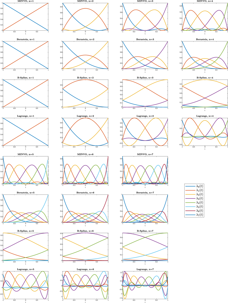
Figure 3: Comparison between the MINVO, Bernstein, B-Spline, and Lagrange bases for $n=1,2,\dots,7$. All these bases satisfy $\sum_{i=0}^{n}\lambda_{i}(t)=1$, and the MINVO, Bernstein, and B-Spline bases also satisfy $\lambda_{i}(t)\geq 0\;\;\forall t\in[-1,1]$.

Table 3: Results for the MINVO basis. $\boldsymbol{A}_{\text{MV}}$, $\boldsymbol{A}_{\text{Be}}$ and $\boldsymbol{A}_{\text{BS}}$ denote the coefficient matrix of the MINVO, Bernstein, and B-Spline bases respectively ($t\in[-1,1]$). The greater the absolute value of the determinant, the smaller the associated simplex (for Problem 1) and the larger the convex hull of the curve (for Problem 2). The matrices $\boldsymbol{A}_{\text{MV}}$ found are independent of the given polynomial curve (in Problem 1), or of the given simplex (in Problem 2). NGO and NLO denote numerical Global/Local Optimality.

$\boldsymbol{n}$	$\boldsymbol{A}_{\text{MV}}$	$\text{abs}\left(\left|\boldsymbol{A}_{\text{MV}}\right|\right)$	$\;\frac{\text{abs}\left(|\boldsymbol{A}_{\text{MV}}|\right)}{\text{abs}\left(|\boldsymbol{A}_{\text{Be}}|\right)}\;$	$\frac{\text{abs}\left(|\boldsymbol{A}_{\text{MV}}|\right)}{\text{abs}\left(|\boldsymbol{A}_{\text{BS}}|\right)}$	Problem 3	Problem 4
$1$	$\frac{1}{2}\left[\begin{array}[]{cc}-1&1\\ 1&1\end{array}\right]$	$0.5$	$1.0$	$1.0$	NGO	NGO
$2$	$\frac{1}{8}\left[\begin{array}[]{ccc}3&-2\sqrt{3}&1\\ -6&0&6\\ 3&2\sqrt{3}&1\end{array}\right]$	$0.3248$	$1.299$	$5.196$	NGO	NGO
$3$	$\left[\begin{array}[]{cccc}-0.4302&0.4568&-0.02698&0.0004103\\ 0.8349&-0.4568&-0.7921&0.4996\\ -0.8349&-0.4568&0.7921&0.4996\\ 0.4302&0.4568&0.02698&0.0004103\end{array}\right]$	$0.3319$	$2.360$	$254.9$	NGO	NGO
$4$	$\left[\begin{array}[]{ccccc}0.5255&-0.5758&-0.09435&0.1381&0.03023\\ -1.108&0.8108&0.9602&-0.8108&0.1483\\ 1.166&0&-1.732&0&0.643\\ -1.108&-0.8108&0.9602&0.8108&0.1483\\ 0.5255&0.5758&-0.09435&-0.1381&0.03023\end{array}\right]$	$0.5678$	$6.057$	$1.675\cdot 10^{5}$	$\begin{array}[]{c}\text{NLO}\\ \text{(at least)}\end{array}$	$\begin{array}[]{c}\text{NLO}\\ \text{(at least)}\end{array}$
$5$	$\left[\begin{array}[]{cccccc}-0.7392&0.7769&0.3302&-0.3773&-0.0365&0.04589\\ 1.503&-1.319&-1.366&1.333&-0.121&0.002895\\ -1.75&0.5424&2.777&-0.9557&-1.064&0.4512\\ 1.75&0.5424&-2.777&-0.9557&1.064&0.4512\\ -1.503&-1.319&1.366&1.333&0.121&0.002895\\ 0.7392&0.7769&-0.3302&-0.3773&0.0365&0.04589\end{array}\right]$	$1.6987$	$22.27$	$1.924\cdot 10^{9}$	$\begin{array}[]{c}\text{Feasible}\\ \text{(at least)}\end{array}$	$\begin{array}[]{c}\text{NLO}\\ \text{(at least)}\end{array}$
$6$	$\left[\begin{array}[]{ccccccc}1.06&-1.134&-0.7357&0.8348&0.1053&-0.1368&0.01836\\ -2.227&2.055&2.281&-2.299&-0.08426&0.2433&0.0312\\ 2.59&-1.408&-4.27&2.468&1.58&-1.081&0.152\\ -2.844&0&5.45&0&-3.203&0&0.5969\\ 2.59&1.408&-4.27&-2.468&1.58&1.081&0.152\\ -2.227&-2.055&2.281&2.299&-0.08426&-0.2433&0.0312\\ 1.06&1.134&-0.7357&-0.8348&0.1053&0.1368&0.01836\end{array}\right]$	$9.1027$	$117.8$	$4.750\cdot 10^{14}$	$\begin{array}[]{c}\text{Feasible}\\ \text{(at least)}\end{array}$	$\begin{array}[]{c}\text{NLO}\\ \text{(at least)}\end{array}$
$7$	$\left[\begin{array}[]{cccccccc}-1.637&1.707&1.563&-1.682&-0.3586&0.4143&-0.006851&2.854\cdot 10^{-5}\\ 3.343&-3.285&-3.947&4.173&0.6343&-0.9385&-0.02111&0.05961\\ -4.053&2.722&6.935&-4.96&-2.706&2.269&-0.2129&0.00535\\ 4.478&-1.144&-9.462&2.469&6.311&-1.745&-1.312&0.435\\ -4.478&-1.144&9.462&2.469&-6.311&-1.745&1.312&0.435\\ 4.053&2.722&-6.935&-4.96&2.706&2.269&0.2129&0.00535\\ -3.343&-3.285&3.947&4.173&-0.6343&-0.9385&0.02111&0.05961\\ 1.637&1.707&-1.563&-1.682&0.3586&0.4143&0.006851&2.854\cdot 10^{-5}\end{array}\right]$	$89.0191$	$902.7$	$\;2.997\cdot 10^{21}$	$\begin{array}[]{c}\text{Feasible}\\ \text{(at least)}\end{array}$	$\begin{array}[]{c}\text{NLO}\\ \text{(at least)}\end{array}$

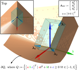
Figure 4: For $n=2$, the MINVO basis has $\boldsymbol{A}_{\text{MV}}=\left[\begin{array}[]{ccc}\boldsymbol{\lambda}_{0}&\boldsymbol{\lambda}_{1}&\boldsymbol{\lambda}_{2}\end{array}\right]^{T}$, where $\boldsymbol{\lambda}_{0},\boldsymbol{\lambda}_{1}$, and $\boldsymbol{\lambda}_{2}$ are vectors that span the parallelepiped , and whose sum is $\left[\begin{array}[]{ccc}0&0&1\end{array}\right]^{T}$. Here, $\partial Q$ ( ) is the frontier of the cone $Q$ formed by the coefficients of the polynomials that are nonnegative for all $t\in[-1,1]$. Note how the globally-optimal vectors $\boldsymbol{\lambda}_{0},\boldsymbol{\lambda}_{1}$, and $\boldsymbol{\lambda}_{2}$ belong to $\partial Q$.

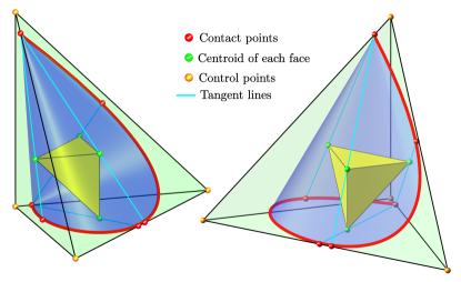
Figure 5: Solution obtained by the MINVO basis for $n=3$. Note how the centroids of each of the facets ( , vertices of the yellow tetrahedron) belong to $\text{conv}\left(P\right)$, which is a necessary condition for an extremal simplex [30]. Moreover, note that $\text{conv}\left(P\right)$ is tangent to the simplex along the blue lines. The red points denote the contact points between the curve and the simplex, which happen at the roots of the MINVO basis functions.

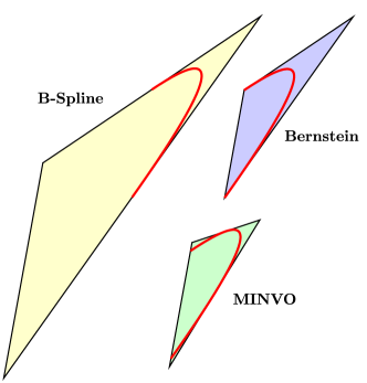
(a) For any given curve $P\in\mathcal{P}^{2}$, the MINVO basis finds an enclosing $2$-simplex that is $1.3$ and $5.2$ times smaller than the one found by the Bernstein and B-Spline bases respectively.

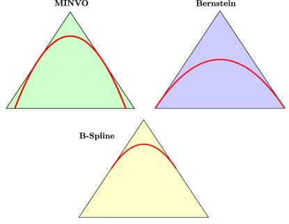
(b) For any given $2$-simplex, the MINVO basis finds a curve $P\in\mathcal{P}^{2}$ inscribed in the simplex, and whose convex hull is $1.3$ and $5.2$ times larger than the one found by the Bernstein and B-Spline bases respectively.

Figure 6: Comparison between the MINVO, Bernstein, and B-Spline bases for $n=2$. The MINVO basis obtains numerically globally optimal results for $n=1,2,3$.

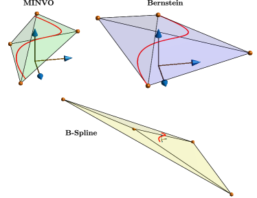
(a) For any given $3^{\text{rd}}$-degree polynomial curve, the MINVO basis finds an enclosing $3$-simplex that is 2.36 and 254.9 times smaller than the one found by the Bernstein and B-Spline bases respectively.

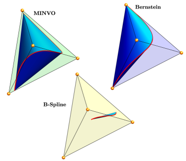
(b) For any given $3$-simplex, the MINVO basis finds a $3^{\text{rd}}$-degree polynomial curve inscribed in the simplex, and whose convex hull is 2.36 and 254.9 times larger than the one found by the Bernstein and B-Spline bases respectively.

Figure 7: Comparison between the MINVO, Bernstein, and B-Spline bases for $n=3$. The MINVO basis obtains numerically globally optimal results for $n=1,2,3$.

One natural question to ask is whether the basis found constitutes a global minimizer for either Problem 3 or Problem 4. To answer this, first note that both Problem 3 and Problem 4 are polynomial optimization problems. Therefore, we can make use of Lasserre’s moment method [61], and increase the order of the moment relaxation to find tighter lower bounds of the original nonconvex polynomial optimization problem. Using this technique, we were able to obtain, for $n=1,2,3$ and for Problem 4, the same objective value as the NLO solutions found before, proving therefore numerical global optimality for these cases. For Problem 3, the moment relaxation technique becomes intractable due to the high number of variables. Hence, to prove numerical global optimality in Problem 3 we instead use the branch-and-bound algorithm, which proves global optimality by reducing to zero the gap between the upper bounds found by a nonconvex solver and the lower bounds found using convex relaxations [62]. This technique proved to be tractable for cases $n=1,2,3$ in Problem 3, and zero optimality gap was obtained.

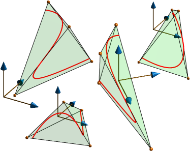
(a) Simplexes found by the MINVO basis for four different given $3^{\text{rd}}$-degree polynomial curves (Problem 1).

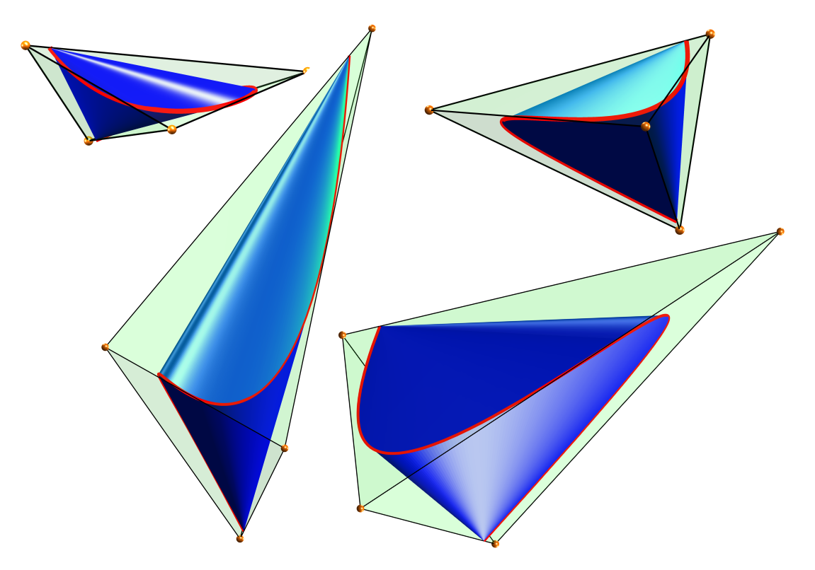
(b) Polynomial curves (and their convex hulls in blue) obtained using the MINVO basis for four different given $3$-simplexes (Problem 2).

Figure 8: MINVO results for $n=3$, where numerical global optimality is guaranteed.

All these results lead us to the following conclusions, which are also summarized in Table 3:

• The matrices $\boldsymbol{A}_{\text{MV}}$ found for $n=1,2,3$ are (numerical) global optima of both Problem 3 and Problem 4.

• The matrix $\boldsymbol{A}_{\text{MV}}$ found for $n=4$ is at least a (numerical) local optimum of both Problem 3 and Problem 4.

• The matrices $\boldsymbol{A}_{\text{MV}}$ found for $n=5,6,7$ are at least (numerical) local optima for Problem 4, and are at least feasible solutions for Problem 3.

The geometric interpretation of Problem 3 (for $n=2$) is shown in Figure 4. The rows of $\boldsymbol{A}$ are vectors that lie in the cone of the polynomials that are nonnegative in $t\in[-1,1]$ (and whose frontier is shown in orange in the figure). As Problem 3 is maximizing the volume of the parallelepiped spanned by these vectors, the optimal minimizer is obtained in the frontier of the cone, while guaranteeing that the sum of these vectors is $\left[\begin{array}[]{ccc}0&0&1\end{array}\right]^{T}$.

In Figure 5 we check that the centroids of each of the facets of the simplex belongs to $\text{conv}\left(P\right)$, which is a necessary condition for that simplex to be minimal [30]. Note also that $\text{conv}\left(P\right)$ is tangent to the simplex along four lines (in blue in the figure), and that the contact points of the curve with the simplex happen at the roots of the MINVO basis functions.

When the polynomial curve is given (i.e., Problem 1), the ratio between the volume of the simplex $S_{\alpha}$ obtained by a basis $\alpha$ and the volume of the simplex $S_{\beta}$ obtained by a basis $\beta$ ($\alpha,\beta\in\{\text{MV},\text{Be},\text{BS}\}$) is given by

$$\frac{\text{vol}\left(S_{\alpha}\right)}{\text{vol}(S_{\beta})}=\frac{\text{abs}(|\boldsymbol{A}_{\beta}|)}{\text{abs}\left(|\boldsymbol{A}_{\alpha}|\right)}\,.$$

Similarly, when the simplex is given (i.e., Problem 2), the ratio between the volume of the convex hull of the polynomial curve $P_{\alpha}$ found by a basis $\alpha$ and the volume of the convex hull of the polynomial curve $P_{\beta}$ found by a basis $\beta$ ($\alpha,\beta\in\{\text{MV},\text{Be},\text{BS}\}$) is given by

$$\frac{\text{vol}\left(\text{conv}\left(P_{\alpha}\right)\right)}{\text{vol}(\text{conv}(P_{\beta}))}=\frac{\text{abs}\left(|\boldsymbol{A}_{\alpha}|\right)}{\text{abs}(|\boldsymbol{A}_{\beta}|)}\,.$$

These ratios are shown in Table 3, and they mean the following for Problem 1 (Problem 2 respectively):

• For $n=3$, the MINVO basis finds a simplex that has a volume (a polynomial curve whose convex hull has a volume) $\approx 2.36$ and $\approx 254.9$ times smaller (larger) than the one the Bernstein and B-Spline bases find respectively.

• For $n=7$, the MINVO basis finds a simplex that has a volume (a polynomial curve whose convex hull has a volume) $\approx 902.7$ and $\approx 2.997\cdot 10^{21}$ times smaller (larger) than the one the Bernstein and B-Spline bases find respectively.

An analogous reasoning applies to the volume ratios of other $n$. These comparisons are shown in Figure 7 (for $n=2$), and in Figure 7 (for $n=3$). More examples of the MINVO bases applied to different polynomial curves and simplexes are shown in Figure 8.

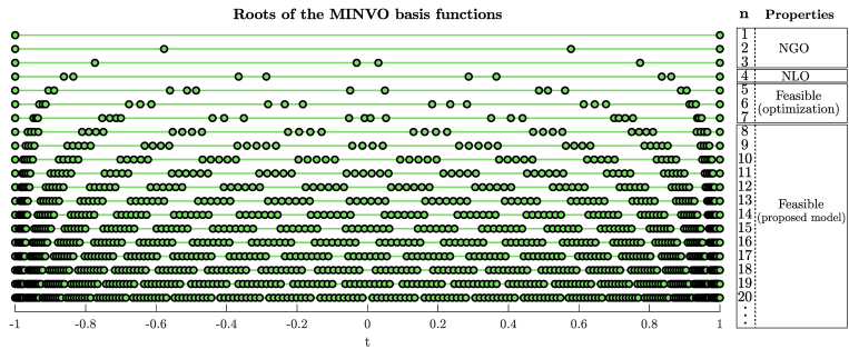
Figure 9: Distribution of the roots of the MINVO basis functions for different $n$. The results for $n\leq 7$ were obtained by solving the optimization problems (Section 6.1, see also Table 2), while the results for $n\geq 8$ were obtained using the model proposed in Section 6.2.

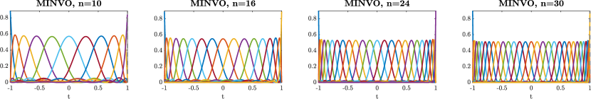
Figure 10: MINVO basis functions obtained for $n=10,16,24,30$ using the model proposed in Section 6.2.

Table 4: Comparison of the results obtained from the optimization (available only for $n=1,\ldots,7$) with the results obtained using the model proposed in Section 6.2 (available for all $n\in\mathbb{N}$). The results obtained using the proposed model are also compared with the Bernstein and B-Spline bases.

		Degree n
		1	2	3	4	5	6	7	8	10	14	18
Opt.	$\text{abs}\left(\left|\boldsymbol{A}_{\text{MV}}\right|\right)$	0.5	0.325	0.332	0.568	1.7	9.1	89.0	-	-	-	-
Proposed model	$\text{abs}\left(\left|\boldsymbol{A}_{\text{MV}}\right|\right)$	0.5	0.325	0.332	0.567	1.69	9.08	88.2	1590.0	3.3e6	2.7e16	5.7e30
	$\log_{10}\text{abs}\left(\frac{\left|\boldsymbol{A}_{\text{MV}}\right|}{\left|\boldsymbol{A}_{\text{Be}}\right|}\right)$	0	0.114	0.373	0.782	1.35	2.07	2.95	4.0	6.57	13.6	23.2
	$\log_{10}\text{abs}\left(\frac{\left|\boldsymbol{A}_{\text{MV}}\right|}{\left|\boldsymbol{A}_{\text{BS}}\right|}\right)$	0	0.716	2.41	5.22	9.28	14.7	21.5	29.7	50.9	113.0	203.0

Table 5: All the possible cases of polynomial curves of degree $n$, dimension $k$, and embedded in a subspace $\mathcal{M}$ of dimension $m$. Note that $m\leq\text{min}(k,n)$ always holds.

		Degree $n$
		1	2	3	4	$\geq 5$
Dimension $k$	1	NGO	F	F	F	F
	2	NGO	NGO	F	F	F
	3	NGO	NGO	NGO	F	F
	4	NGO	NGO	NGO	NLO	F
	$\geq 5$	NGO	NGO	NGO	NLO	F
In all the cases (and for any $m$): there are $n+1$ control points, and conv(control points) is a polyhedron $\subset\mathcal{M}\subseteq\mathbb{R}^{k}$ that encloses the curve and that has at most $n+1$ vertices.

In and below the diagonal: When $n=m$, the polyhedron is an $n$-simplex embedded in $\mathbb{R}^{k}$ that is at least numerically globally optimal (NGO), numerically locally optimal (NLO), or feasible (F).

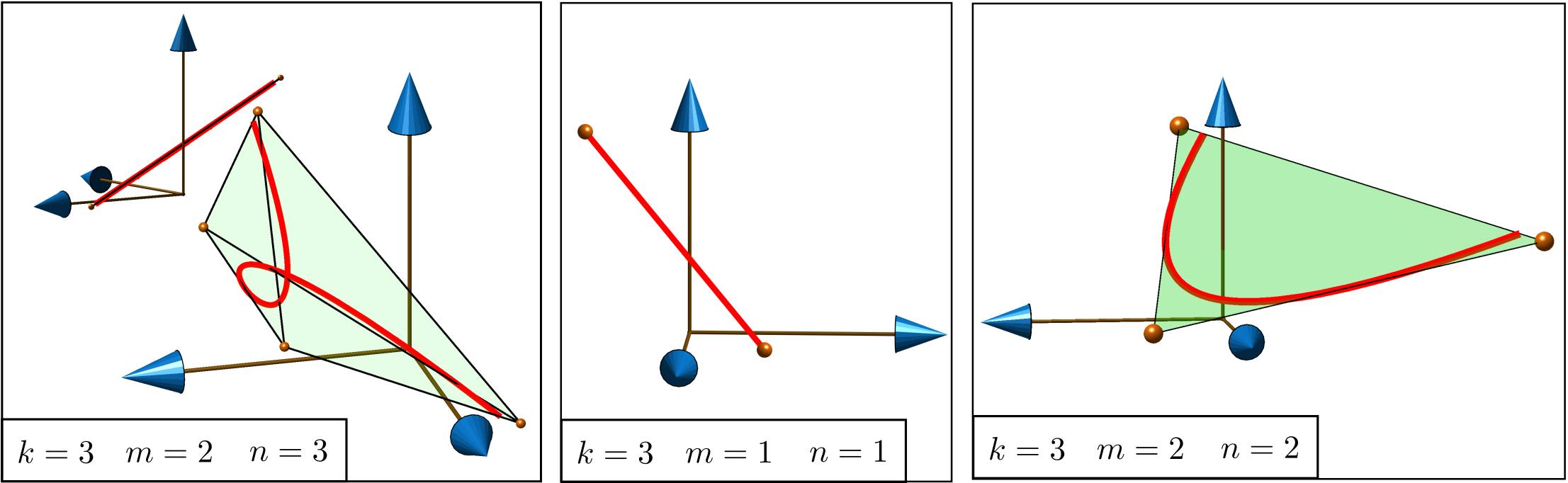
Figure 11: The MINVO basis applied for different curves with $k=3$ and different values of $m$ and $n$: A cubic curve embedded in a two-dimensional subspace (left), a segment embedded in a one-dimensional subspace (middle) and a quadratic curve embedded in a two-dimensional subspace (right).

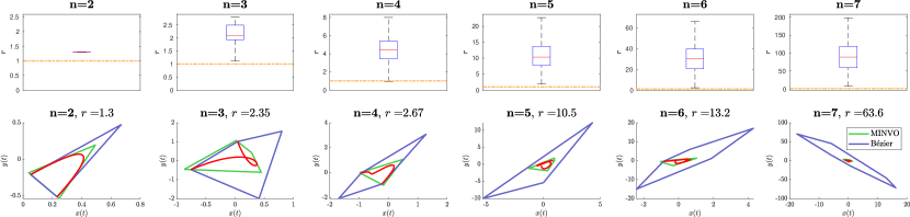
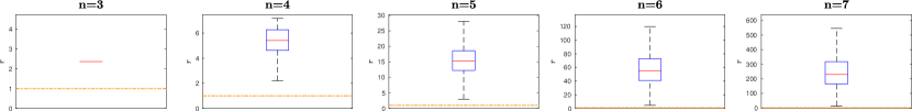
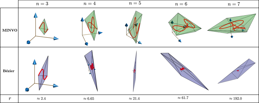
Figure 12: Comparison of the convex hull of the MINVO and Bézier control points for $k=m=2$ and different $n$. Here $r$ denotes the ratio of the areas $\frac{\text{Area}_{\text{Be}}}{\text{Area}_{\text{MV}}}$. The boxplots (top) have been obtained from $10^{4}$ polynomials passing through $n+1$ random points in the square $[-1,1]^{2}$. The yellow dashed line highlights the value $r=\frac{\text{Area}_{\text{Be}}}{\text{Area}_{\text{MV}}}=1$. Some of these random curves and the associated convex hulls are shown at the bottom.

Figure 13: Comparison of the convex hull of the MINVO and Bézier control points for $k=m=3$ and different $n$. Here $r$ denotes the ratio of the volumes $\frac{\text{Vol}_{\text{Be}}}{\text{Vol}_{\text{MV}}}$. The boxplots (top) have been obtained from $10^{4}$ polynomial curves passing through $n+1$ random points in the cube $[-1,1]^{3}$ were used. The yellow dashed line highlights the value $r=\frac{\text{Vol}_{\text{Be}}}{\text{Vol}_{\text{MV}}}=1$. Some of these random curves and the associated convex hulls are shown at the bottom.

6.2 Results for $n>7$

In Section 6.1, we obtained the results for $n=1,\ldots,7$ by using the optimization problems. However, solving these problems becomes intractable when $n>7$. To address this problem, we present a model that finds high-quality feasible solutions by extrapolating for $n>7$ the pattern found for the roots of the MINVO basis (see the cases $n=1,\ldots,7$ in Figure 9). Specifically, and noting that the double roots for a degree $n$ tend to be distributed in $n$ clusters, we found that the MINVO double roots in the interval $(-1,1)$ for the degree $n$ can be approximated by

$$\sin\left(\frac{c_{0}\left(k-\frac{s_{j,n}-1}{2}\right)+c_{1}\left(j-\frac{n-1}{2}\right)}{n+c_{2}}\right)\,,$$ (4)

where $s_{j,n}:=\left\lfloor\frac{n+\text{odd}\left(j,n\right)}{2}\right\rfloor$ models the number of roots per cluster $j\in\{0,\ldots,(n-1)\}$, and $k\in\{0,\ldots,(s_{j,n}-1)\}$ is the index of the root inside a specific cluster.

Here, $c_{0}\approx 0.2735$, $c_{1}\approx 3.0385$, and $c_{2}\approx 0.4779$ were found by optimizing the associated nonlinear least-squares problem. This proposed model, with only three parameters, is able to obtain a least-square residual of $5.02\cdot 10^{-3}$ with respect to the MINVO roots lying in $(-1,1)$ found for $n=2,\ldots,7$. The distribution of roots generated by this proposed model ($n\geq 8$) is shown in Figure 9. Each root can then be assigned to a polynomial $i$ of the basis by simply following the same assignment pattern found for $n=1,...,7$. Then, and by solving a linear system, the polynomials can be scaled to enforce $\sum_{i=0}^{n}\lambda_{i}(t)=1\;\forall t$ (or equivalently, $\boldsymbol{A}^{T}\boldsymbol{1}=\boldsymbol{e}$). Note that this proposed model, although not guaranteed to be optimal, is guaranteed to be feasible by construction. Some examples of the MINVO basis functions are shown in Figure 10. The comparison of $\left|\boldsymbol{A}_{\text{MV}}\right|$ between the proposed model and the optimization results of Section 6.1 is shown in Table 4. For $n=1,\ldots,7$, the relative error between the objective value obtained using the optimization and the one obtained using the proposed model is always $<9.2\cdot 10^{-3}$. The proposed model also produces much smaller simplexes than the Bernstein and B-Spline bases.

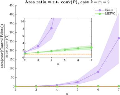
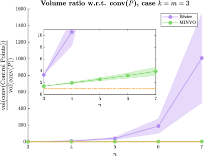
Figure 14: Comparison of the convex hull of the MINVO and Bézier control points with respect to $\text{conv}(P)$ for the cases $k=m=2$ (left) and $k=m=3$ (right). For each $n$, a total of $10^{3}$ polynomial curves passing through $n+1$ random points in the cube $[-1,1]^{k}$ were used. The shaded area is the 1$\sigma$ interval, where $\sigma$ is the standard deviation. The yellow dashed line marks a ratio of 1. Note how the growth of the ratio for the MINVO basis is approximately linear with $n$, while for the Bézier basis it is approximately exponential.

7 MINVO basis applied to other curves

7.1 Polynomial curves of degree $n$, dimension $k$, and embedded in a subspace $\mathcal{M}$ of dimension $m$

So far we have studied the case of $n=m=k$ (i.e., a polynomial curve of degree $n$ and dimension $k=n$ and for which $n$ is also the dimension of $\mathcal{M}$, see Section 3.1). The most general case would be any $k,n$ and $m$, as shown in Table 5. In all these cases, and using the $(n+1)\times(n+1)$ matrix $\boldsymbol{A}_{\text{MV}}$, we can still apply the equation $\boldsymbol{V}_{k\times(n+1)}=\boldsymbol{P}_{k\times(n+1)}\boldsymbol{A}_{\text{MV}}^{-1}$ to obtain all the $n+1$ MINVO control points in $\mathbb{R}^{k}$ of the given curve (columns of the matrix $\boldsymbol{V}$). The convex hull of the control points is a polyhedron that is guaranteed to contain the curve because the curve is a convex combination of the control points. Note also that, when $n=m$, all the cases below the diagonal of Table 5 have the same optimality properties (NGO/NLO/Feasible) as the diagonal element that has the same $n$.

For $k=3$, Figure 11 shows a cubic curve embedded in a two-dimensional subspace ($m=2$, $n=3$), a segment embedded in a one-dimensional subspace ($m=n=1$) and a quadratic curve embedded in a two-dimensional subspace ($m=n=2$).

For $k=m=2$, the comparison between the area of the convex hull of the MINVO control points ($\text{Area}_{\text{MV}}$) and the area of the convex hull of the Bézier control points ($\text{Area}_{\text{Be}}$) is shown in Figure 13. Note that this ratio is constant for any polynomial curve for the case $n=2$, but depends on the given curve for the cases $n>2$. To generate the boxplots of Figure 13, we used a total of $10^{4}$ polynomial curves passing through $n+1$ points randomly sampled from the square $[-1,1]^{2}$. Although it is not guaranteed that $\text{Area}_{\text{MV}}<\text{Area}_{\text{Be}}$ for any polynomial with $n>2$, the Monte Carlo analysis performed using these random polynomial curves shows that $\text{Area}_{\text{MV}}<\text{Area}_{\text{Be}}$ holds for the great majority of them, with improvements up to $\approx 200$ times for the case $n=7$.

Similarly, the results for $k=m=3$ are shown in Figure 13, where we used a total of $10^{4}$ polynomial curves passing through $n+1$ points randomly sampled from the cube $[-1,1]^{3}$. Again, it is not guaranteed that $\text{Vol}_{\text{MV}}<\text{Vol}_{\text{Be}}$ for any polynomial with $n>3$, but the Monte Carlo results obtained show that this is true in most of these random polynomials. For the case $n=7$, the MINVO basis obtains convex hulls up to $\approx 550$ times smaller than the Bézier basis.

Qualitatively, and for the comparisons shown above, the MINVO enclosures are much smaller than the Bézier enclosures when used in “tangled” curves. In these curves, the Bézier control points tend to be spread out and far from the curve, leading therefore to large and conservative Bézier enclosures.

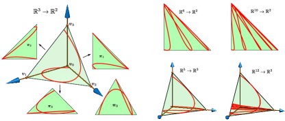
Figure 15: The MINVO basis also obtains simplexes that tightly enclose some rational curves (curves whose coordinates are the quotient of two polynomials). On the left, the standard simplex is the smallest 3-simplex containing the 3D curve in red. This means that each facet $i$ (contained in the plane $\boldsymbol{\pi}_{i}$) is also the smallest 2-simplex enclosing the projection of the curve onto that facet using the opposite vertex $\boldsymbol{v}_{i}$ as viewpoint. On the right, different successive projections to $\mathbb{R}^{2}$ and $\mathbb{R}^{3}$ are shown.

Finally, we compare in Figure 14 how these polyhedral convex hulls, obtained by either the MINVO or Bézier control points, approximate $\text{conv}(P)$, which is the convex hull of the curve $P$. Similar to the previous cases, here we used a total of $10^{3}$ polynomial curves passing through $n+1$ points randomly sampled from the cube $[-1,1]^{k}$. The error in the MINVO outer polyhedral approximation is approximately linear as $n$ increases, but it is exponential for the Bézier basis. For instance, when $n=7$ and $k=3$, the Bézier control points generate a polyhedral outer approximation that is $\approx 1010$ times larger than the volume of $\text{conv}(P)$, while the polyhedral outer approximation obtained by the MINVO control points is only $\approx 3.9$ times larger.

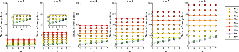
Figure 16: Comparison of the number of raw points produced by the MINVO (MV) enclosure, Bézier (Be) enclosure, and SLEFE (SL) for $n^{\text{th}}$-degree 2D polynomial curves. Here, $s$ is the number of subintervals the curve is divided into and SL_$h$ denotes the SLEFE computed using $h$ breakpoints per subinterval (i.e., $h-1$ linear segments per subinterval). The MINVO enclosures have fewer raw points than all SL_$h$ ($h\in[2,8]$) for $n\in[2,6]$. Compared to Bézier, the MINVO enclosure has $s-1$ additional raw points, but achieves areas that are up to $30$ times smaller (see Figure 23).

7.2 Rational Curves

Via projections, the MINVO basis is also able to obtain the smallest simplex that encloses some rational curves, which are curves whose coordinates are the quotients of two polynomials. For instance, given the $n$-simplex obtained by the MINVO basis for a given $n^{\text{th}}$-degree polynomial curve $P$, we can project every point $\boldsymbol{p}(t)$ of the curve via a perspective projection, using a vertex as the viewpoint, and the opposite facet as the projection plane. Note that this perspective projection of the polynomial curve will be a rational curve. If the $n$-simplex is the smallest one enclosing the polynomial curve, then each facet is also the smallest $(n-1)$-simplex that encloses the projection. This can be easily proven by contradiction, since if the facet were not a minimal $(n-1)$-simplex for the projected curve, then the $n$-simplex would not be minimal for the original 3D curve (see [63] for instance). Let us define $\left[\begin{array}[]{ccc}\boldsymbol{v}_{0}&\ldots&\boldsymbol{v}_{n}\end{array}\right]:=\left[\begin{array}[]{cc}\boldsymbol{0}&\boldsymbol{I}_{n}\end{array}\right]$, and let $\boldsymbol{\pi}_{i}$ denote the plane that passes though the vertices $\{\boldsymbol{v}_{0},\boldsymbol{v}_{1},\ldots,\boldsymbol{v}_{n}\}\backslash\{\boldsymbol{v}_{i}\}$. Then, for a standard $n$-simplex, the perspective projection of $\boldsymbol{p}(t):=\left[\begin{array}[]{ccc}\boldsymbol{\lambda}_{1}&\cdots&\boldsymbol{\lambda}_{n}\end{array}\right]^{T}\boldsymbol{t}$ onto the plane $\boldsymbol{\pi}_{i}$, using $\boldsymbol{v}_{i}$ as the viewpoint, is given by:

$$\begin{cases}\frac{1}{1-\boldsymbol{\lambda}_{0}^{T}\boldsymbol{t}}\left[\begin{array}[]{ccc}\boldsymbol{\lambda}_{1}&\cdots&\boldsymbol{\lambda}_{n}\end{array}\right]^{T}\boldsymbol{t}&\text{Projection onto $\boldsymbol{\pi}_{0}$}\\ \frac{1}{1-\boldsymbol{\lambda}_{i}^{T}\boldsymbol{t}}\left[\begin{array}[]{cccccc}\boldsymbol{\lambda}_{1}\cdots&\boldsymbol{\lambda}_{i-1}&0&\boldsymbol{\lambda}_{i+1}&\cdots&\boldsymbol{\lambda}_{n}\end{array}\right]^{T}\boldsymbol{t}&\text{\text{Projection onto }}\boldsymbol{\pi}_{i},i>0\end{cases}$$

This projection can also be applied successively from $\mathbb{R}^{i}$ to $\mathbb{R}^{j}$ ($i>j\geq 1$). Figure 15 shows the case $\mathbb{R}^{3}\rightarrow\mathbb{R}^{2}$ (for all the four possible projections), and some projections of the cases $\mathbb{R}^{6}\rightarrow\mathbb{R}^{2}$, $\mathbb{R}^{10}\rightarrow\mathbb{R}^{2}$, $\mathbb{R}^{5}\rightarrow\mathbb{R}^{3}$, and $\mathbb{R}^{12}\rightarrow\mathbb{R}^{3}$.

8 Comparison with SLEFEs

In this section, we compare the enclosures for $n^{\text{th}}$-degree 2D polynomial curves obtained using these three techniques with and without subdivision:

• MINVO: The curve is divided into $s$ subintervals, and then the MINVO enclosure for each of the subintervals is computed.

• Bézier: The curve is divided into $s$ subintervals, and then the Bézier enclosure for each of the subintervals is computed.

• SLEFE: The curve is divided into $s$ subintervals, and the SLEFE (subdividable linear efficient function enclosure [64, 26, 24]) is obtained using $h$ breakpoints per subinterval (i.e., $h-1$ linear segments per subinterval). A SLEFE obtained with $h$ breakpoints per subinterval will be denoted as SL_$h$.

Note that $s=1$ corresponds to the case where no subdivision is performed. When $s>1$, the subintervals of the curve are obtained by evenly splitting the time interval. Moreover, SL_$2$ (i.e., $h=2$) corresponds to a SLEFE with only one linear segment (i.e., two breakpoints) per subinterval.

We compare the width, the union, and the convex hull (defined in F) for the different enclosures. The comparison of the width of the enclosures produced is available in G. The comparison of the area and number of vertices of the union and the convex hull is available in H. In I, we compare MINVO and SLEFE in terms of runtime and simplicity of their implementation.

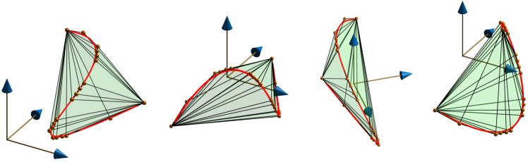
Figure 17: Tighter polyhedral outer approximations for a curve $P\in\mathcal{P}^{n}$ can be obtained by splitting the curve into several subintervals, calculating the MINVO $n$-simplexes that enclose each one of these subintervals and then computing the convex hull of all these simplexes. In all these cases shown, the original curve $P\in\mathcal{P}^{3}$ is splitted into $5$ subintervals (i.e., $s=5$), and the resulting convex hull is a polyhedron with $20$ vertices that is $1.19$ times smaller than the smallest 3-simplex that encloses the whole curve (i.e., the simplex found by applying the MINVO basis to the whole curve).

Several conclusions can be drawn regarding the comparison between MINVO, Bézier, and SLEFE:

• Compared to SL_$2$, MINVO achieves a smaller area for most of the $n$–$s$ combinations tested, and sometimes using only half of the vertices needed by SL_$2$. Compared to SL_$h$ ($h\in[3,8]$), MINVO typically achieves a smaller area for the cases where either $s$ is small or the degree $n$ is high, and it usually does so using fewer number of vertices than SL_$h$. On the other hand, SL_$h$ tends to achieve a smaller area when either $s$ is large or the degree $n$ is small, but it usually requires more vertices than MINVO. Hence, MINVO is advantageous with respect to SL_$h$ in applications where having a small number of vertices is crucial. For example, a smaller number of vertices can substantially reduce the total computation time in algorithms that, after finding the enclosure, need to iterate through all of the vertices found to impose a constraint or perform a specific operation/check for each of them. If the number of vertices is not important for the specific application, then SL_$h$ ($h\geq 4$) should be chosen, since it typically achieves a smaller area of the union and area of the convex hull.

• Compared to Bézier, MINVO also achieves a smaller union and hull area for the cases where either $s$ is small or the degree $n$ is high, and, when $n\in[3,7]$, it does so using only up to $1.3$ times the number of vertices of Bézier.

• In terms of the width of the enclosure (G), SLEFE performs better than MINVO. The use of SLEFE is hence desirable in the cases where the width of the enclosure is more important for the specific application.

• For any of the techniques, operations like the union, the convex hull, or the outer boundaries computation for SLEFE ([24]) are typically either not possible or computationally expensive in the applications where the curve itself is a decision variable of an optimization problem (as in, e.g., [65, 66, 12, 13]). Instead, we can use the raw points of the enclosure, which in 2D can be defined as the unique control points of each subinterval (for MINVO and Bézier), and as the unique vertices of each of the rectangles generated per breakpoint of each subinterval (for SL_$h$). The number of these raw points for a general 2D curve is $ns+s$ for MINVO, $ns+1$ for Bézier, and $4hs$ for SL_$h$. The comparison of these raw points is shown in Figure 16. The MINVO enclosures have fewer raw points than all SL_$h$ ($h\in[2,8]$) for $n\in[2,6]$. Compared to Bézier, the MINVO enclosure has $s-1$ additional raw points, but achieves areas that are up to $30$ times smaller (see Figure 23).

• As noted in [24], SLEFE depends pseudo-linearly on the coefficients of the polynomial curve (i.e., linearly except for a min/max operation). In contrast, the MINVO or Bézier enclosures depend linearly on the coefficients of the polynomial curve. This makes the MINVO and Bézier enclosures more suitable for time-critical optimization problems in which the coefficients of the curve are decision variables.

9 Final Remarks

9.1 Conversion between MINVO, Bernstein, and B-Spline

Given a curve $P\in\mathcal{P}^{n}$, the control points (i.e., the vertices of the $n$-simplex that encloses that curve) using a basis $\alpha$ can be obtained from the control points of a different basis $\beta$ ($\alpha,\beta\in\{\text{MV},\text{Be},\text{BS}\}$) using the formula

$$\boldsymbol{V}_{\alpha}=\boldsymbol{P}\boldsymbol{A}_{\alpha}^{-1}=\boldsymbol{V}_{\beta}\boldsymbol{A}_{\beta}\boldsymbol{A}_{\alpha}^{-1}\,.$$ (5)

For instance, to obtain the Bernstein control points from the MINVO control points we can use $\boldsymbol{V}_{\text{Be}}=\boldsymbol{V}_{\text{MV}}\boldsymbol{A}_{\text{MV}}\boldsymbol{A}_{\text{Be}}^{-1}$. The matrices $\boldsymbol{A}_{\text{MV}}$ are the ones shown in Table 3, while the matrices $\boldsymbol{A}_{\text{Be}}$ and $\boldsymbol{A}_{\text{BS}}$ are available in [48]. Note that all the matrices need to be expressed in the same interval ($t\in[-1,1]$ in this paper), and that the inverses of these matrices can be easily precomputed offline.

9.2 Tighter volumes for Problem 1 via subdivision

As shown in Section 8, and at the expense of adding more vertices, tighter polyhedral solutions for Problem 1 can be obtained by dividing the polynomial curve into several subintervals and then computing the convex hull of the MINVO enclosure of each subinterval. To subdivide the curve, one can do it first in Bézier form (leveraging therefore the properties of De Casteljau’s algorithm), and then compute the MINVO control points as linear functions of the Bézier control points of that subinterval using Eq. 5. Alternatively, one can also tabulate (offline) the inverse of the matrices $\boldsymbol{A}_{\text{MV}}$, expressed in the subinterval desired, and then simply compute the MINVO control points of that subinterval as $\boldsymbol{V}_{\text{MV}}=\boldsymbol{P}\boldsymbol{A}_{\text{MV}}^{-1}$.

Several examples for $n=3$ are shown in Figure 17, where the original curve $P\in\mathcal{P}^{3}$ is split into $5$ subintervals (i.e., $s=5$), and the resulting convex hull is a polyhedron with $20$ vertices that is $1.19$ times smaller than the smallest 3-simplex that encloses the whole curve (i.e., the simplex found by applying the MINVO basis to the whole curve).

Depending on the specific application, one might also be interested in obtaining a sequence of overlapping polyhedra whose union (a nonconvex set in general) completely encloses the curve. This can be obtained by simply computing the MINVO enclosure for every subinterval of the curve.

9.3 When should each basis be used?

The Bernstein (Bézier) and B-Spline bases have many useful properties that are not shared by the MINVO basis. For example, a polynomial curve passes through the first and last Bézier control points, the derivative of a Bézier curve can be easily computed from the difference of the Bézier control points, and the B-Spline basis has built-in smoothness in curves with several segments. Hence, it may be desirable to use the Bézier or B-Spline control points to design and model the curve, and then convert the control points of every interval to the MINVO control points (using the simple linear transformation given in Section 9.1) to perform collision/intersection checks, or to impose collision-avoidance constraints in an optimization problem [18, 12, 13]. This approach benefits from the properties of the Bernstein/B-Spline bases, while also exploiting the enclosures obtained by the MINVO basis.

10 Conclusions and Future Work

This work derived and presented the MINVO basis. The key feature of this basis is that it finds the smallest $n$-simplex that encloses a given $n^{\text{th}}$-degree polynomial curve (Problem 1), and also finds the $n^{\text{th}}$-degree polynomial curve with largest convex hull enclosed in a given $n$-simplex (Problem 2). For $n=3$, the ratios of the improvement in the volume achieved by the MINVO basis with respect to the Bernstein and B-Spline bases are $2.36$ and $254.9$ respectively. When $n=7$, these improvement ratios increase to $902.7$ and $2.997\cdot 10^{21}$ respectively. Numerical global optimality was proven for $n=1,2,3$, numerical local optimality was proven for $n=4$, and high-quality feasible solutions for all $n\geq 5$ were obtained. Finally, the MINVO basis was also applied to polynomial curves with different $n$, $k$ and $m$ (achieving improvements ratios of up to $\approx 550$), and to some rational curves.

The exciting results of this work naturally lead to the following questions and conjectures, that we leave as future work:

• Is the global optimum of Problem 4 the same as the global optimum of Problem 3? I.e., are we losing optimality by imposing the specific structure on $\lambda_{i}(t)$? On a similar note, is it possible to obtain for any $n$ a bound on the distance between the objective value obtained by the model proposed in Section 6.2, and the global minimum of Problem 3?

• Does there exist a recursive formula to obtain the solution of Problem 3 for a specific $n=q$ given the previous solutions for $n=1,\ldots,q-1$? Would this recursive formula allow to obtain the globally optimal solutions for all $n\in\mathbb{N}$ of Problem 3?

Finally, the way polynomials are scaled (to impose $\boldsymbol{A}^{T}\boldsymbol{1}=\boldsymbol{e}$) in Section 6.2 can suffer from numerical instabilities when the degree is very high ($n>30$). This is expected, since the monomial basis used to compute $\boldsymbol{A}$ is known to be numerically unstable [53]. A more numerically-stable scaling, potentially avoiding the use of the monomial basis, could therefore be beneficial for higher degrees.

Acknowledgments

The authors would like to thank Prof. Gilbert Strang, Prof. Luca Carlone, Dr. Ashkan M. Jasour, Dr. Kasra Khosoussi, Dr. David Rosen, Juan José Madrigal, Parker Lusk, Dr. Kris Frey, and Dr. Maodong Pan for helpful insights and discussions. The authors would also like to thank the anonymous reviewers, whose valuable feedback helped to improve the article. Research funded in part by Boeing Research & Technology.

Appendix A Volume of the Convex Hull of a Polynomial Curve

The volume of the convex hull of any $n^{\text{th}}$-degree polynomial curve can be easily obtained using the result from [45, Theorem 15.2]. In this work, it is shown that the volume of the convex hull of a curve $R$ with $\boldsymbol{r}(t):=\left[\begin{array}[]{cccc}\frac{t+1}{2}&\left(\frac{t+1}{2}\right)^{2}&\cdots&\left(\frac{t+1}{2}\right)^{n}\end{array}\right]^{T}$ is given by vol(conv(R))=∏_j=1^nB(j,j)=∏_j=1^n(((j-1)!)2(2j-1)!)=1n!∏_j=1^n(j!(j-1)!(2j-1)!)=1n!∏_0≤i<j≤n(j-ij+i)   , where $\text{B}(x,y)$ denotes the beta function. Let us now define $\tilde{\boldsymbol{t}}$ as $\tilde{\boldsymbol{t}}:=\left[\begin{array}[]{cccc}t^{n}&t^{n-1}&\cdots&t\end{array}\right]^{T}$, $\boxtimes$ as any number in $\mathbb{R}$ and write $\boldsymbol{r}(t)$ as:

$$\boldsymbol{r}(t)=\underbrace{\left[\begin{array}[]{cccccc}0&0&\cdots&0&\frac{1}{2}&\boxtimes\\ 0&0&\cdots&\frac{1}{2^{2}}&\boxtimes&\boxtimes\\ \vdots&\vdots&\ddots&\vdots&\vdots&\vdots\\ 0&\frac{1}{2^{n-1}}&\cdots&\boxtimes&\boxtimes&\boxtimes\\ \frac{1}{2^{n}}&\boxtimes&\cdots&\boxtimes&\boxtimes&\boxtimes\end{array}\right]}_{:=\boldsymbol{R}}\boldsymbol{t}=\boldsymbol{R}_{:,0:n-1}\tilde{\boldsymbol{t}}+\boldsymbol{R}_{:,n}$$

Now, defining $\boldsymbol{Q}:=\boldsymbol{P}_{:,0:n-1}\boldsymbol{R}_{:,0:n-1}^{-1}$, note that $\left(\boldsymbol{p}(t)-\boldsymbol{P}_{:,n}\right)=\boldsymbol{P}_{:,0:n-1}\tilde{\boldsymbol{t}}=\boldsymbol{Q}\boldsymbol{R}_{:,0:n-1}\tilde{\boldsymbol{t}}=\boldsymbol{Q}\left(\boldsymbol{r}(t)-\boldsymbol{R}_{:,n}\right)=\boldsymbol{Q}\boldsymbol{r}(t)-\boldsymbol{Q}\boldsymbol{R}_{:,n}$. As the translation part does not affect the volume, we can write vol(conv(P))=vol(conv({ p(t)-P_:,n | t∈[-1,1]} ))=vol(conv({ Qr(t) | t∈[-1,1]} ))=…

$$...=\text{vol}\left(\boldsymbol{Q}\text{conv}\left(R\right)\right)=\text{abs}\left(\frac{\left|\boldsymbol{P}_{:,0:n-1}\right|}{\left|\boldsymbol{R}_{:,0:n-1}\right|}\right)\text{vol}\left(\text{conv}\left(R\right)\right)\,,$$

where we have used the notation $\boldsymbol{Q}\text{conv}\left(R\right)$ to denote the set $\left\{\boldsymbol{Q}\boldsymbol{x}|\boldsymbol{x}\in\text{conv}\left(R\right)\right\}$.

As the determinant of $\boldsymbol{R}_{:,0:n-1}$ is $\left|\boldsymbol{R}_{:,0:n-1}\right|=\prod_{i=1}^{n}\frac{1}{2^{i}}=2^{\frac{-n(n+1)}{2}}$, we can conclude that:

$$\boxed{\text{vol}\left(\text{conv}\left(P\right)\right)=\frac{\text{abs}\left(\left|\boldsymbol{P}_{:,0:n-1}\right|\right)}{n!}2^{\frac{n(n+1)}{2}}\prod_{0\leq i<j\leq n}\left(\frac{j-i}{j+i}\right)}$$

$\square$

Appendix B Invertibility of the matrix $\boldsymbol{A}$

From Eq. 3, we have that the $(n+1)\times(n+1)$ matrix $\boldsymbol{A}$ satisfies

$$\left[\begin{array}[]{c}\boldsymbol{P}\\ \boldsymbol{e}^{T}\end{array}\right]=\left[\begin{array}[]{c}\boldsymbol{V}\\ \boldsymbol{1}^{T}\end{array}\right]\boldsymbol{A}\,.$$

As $\text{abs}\left(\left|\begin{array}[]{c}\boldsymbol{P}\\ \boldsymbol{e}^{T}\end{array}\right|\right)=\text{abs}\left(\left|\boldsymbol{P}_{:,0:n-1}\right|\right)\neq 0$, and $\left|\begin{array}[]{c}\boldsymbol{V}\\ \boldsymbol{1}^{T}\end{array}\right|=\left|\begin{array}[]{cc}\boldsymbol{V}^{T}&\boldsymbol{1}\end{array}\right|\neq 0$ (see Section 4), we have that $\text{rank}\left(\left[\begin{array}[]{c}\boldsymbol{P}\\ \boldsymbol{e}^{T}\end{array}\right]\right)=\text{rank}\left(\left[\begin{array}[]{c}\boldsymbol{V}\\ \boldsymbol{1}^{T}\end{array}\right]\right)=n+1$. Using now the fact that $\text{rank}\left(\boldsymbol{B}\boldsymbol{C}\right)\leq\min\left(\text{rank}\left(\boldsymbol{B}\right),\text{rank}\left(\boldsymbol{C}\right)\right)$, we conclude that $\text{\text{rank}$\left(\boldsymbol{A}\right)$}=n+1$ (i.e., $\boldsymbol{A}$ has full rank), and therefore $\boldsymbol{A}$ is invertible. $\square$

Appendix C Karush–Kuhn–Tucker conditions (for odd $n$)

In this Appendix we derive the KKT conditions for this problem:

$$\framebox{$\begin{array}[]{c}\underset{\boldsymbol{A}\in\mathbb{R}^{(n+1)\times(n+1)}}{\min}\quad-\text{ln}\left(\left|\boldsymbol{A}^{T}\boldsymbol{A}\right|\right)\\ \text{s.t.}\quad\;\boldsymbol{A}^{T}\boldsymbol{1}=\boldsymbol{e}\\ \qquad\qquad\boldsymbol{A}\boldsymbol{t}\geq\boldsymbol{0}\quad\forall t\in[-1,1]\end{array}$}$$

which is equivalent to Problem 3. For the sake of brevity, we present here the case $n$ odd (the case $n$ even can be easily obtained with small modifications). In the following, $\boldsymbol{V}*\boldsymbol{W}$ will be the matrix resulting from the row-wise discrete convolution (i.e., $\left(\boldsymbol{V}*\boldsymbol{W}\right)_{i,:}=\boldsymbol{V}_{i,:}*\boldsymbol{W}_{i,:}$), and $\text{Top}(\boldsymbol{a},\boldsymbol{b})$ will denote the Toeplitz matrix whose first column is $\boldsymbol{a}$ and whose first row is $\boldsymbol{b}^{T}$. Let us also define:

and the matrices $\boldsymbol{G}\in\mathbb{R}^{(n+1)\times\frac{n+1}{2}}$, $\boldsymbol{H}\in\mathbb{R}^{(n+1)\times\frac{n+1}{2}}$ and $\boldsymbol{\lambda}\in\mathbb{R}^{(n+1)}$. We know that

$$\text{...$\iff\boldsymbol{A}$=$\left[\begin{array}[]{c|c}\boldsymbol{G}*\boldsymbol{G}&\boldsymbol{H}*\boldsymbol{H}\end{array}\right]\left[\begin{array}[]{c}\boldsymbol{R}_{G}^{T}\\ \boldsymbol{R}_{H}^{T}\end{array}\right]$}\,,$$ (6)

where $g_{i}(t)$ and $h_{i}(t)$ are polynomials of degree $\frac{n-1}{2}$. Note that (a) is given by the Markov–Lukács Theorem (see Section 5.4). In (b) we have simply used the discrete convolution to multiply $g_{i}(t)$ by itself, and the Toeplitz matrix $\boldsymbol{R}_{\boldsymbol{G}}$ to multiply the result by $(t+1)$ [48]. An analogous reasoning applies for the term with $h_{i}$. Using now $\boldsymbol{G}$ and $\boldsymbol{H}$ as the decision variables of the primal problem (where $\boldsymbol{A}$ is given by Eq. 6), the Lagrangian is $\mathcal{L=}-\text{ln}(|\boldsymbol{A}^{T}\boldsymbol{A}|)+\boldsymbol{\lambda}^{T}(\boldsymbol{A}^{T}\boldsymbol{1}-\boldsymbol{e})$   .

Differentiating the Lagrangian yields to

$$\frac{\partial\mathcal{L}}{\partial\boldsymbol{G}_{ij}}=\text{tr}\left(-\underbrace{\frac{\partial\text{ln}\left(\left|\boldsymbol{A}^{T}\boldsymbol{A}\right|\right)}{\partial\boldsymbol{A}}}_{=2\boldsymbol{A}^{+}=2\boldsymbol{A}^{-1}}\boldsymbol{Q}_{\boldsymbol{G}_{ij}}\right)+\text{tr}\left(\boldsymbol{\lambda}\boldsymbol{1}^{T}\boldsymbol{Q}_{\boldsymbol{G}_{ij}}\right)=\text{tr}\left(\left(-2\boldsymbol{A}^{-1}+\boldsymbol{\lambda}\boldsymbol{1}^{T}\right)\boldsymbol{Q}_{\boldsymbol{G}_{ij}}\right)\,,$$

where

$$\boldsymbol{Q}_{\boldsymbol{G}_{ij}}:=\frac{\partial\boldsymbol{A}}{\partial\boldsymbol{G}_{ij}}=2\left(\boldsymbol{L}_{(n+1)}\right)^{i-1}\left[\begin{array}[]{c}\left[\begin{array}[]{cc}\boldsymbol{G}_{i,:}&\boldsymbol{0}^{T}\end{array}\right]\left(\boldsymbol{L}_{n}^{T}\right)^{j-1}\boldsymbol{R}_{\boldsymbol{G}}^{T}\\ \boldsymbol{0}_{n\times(n+1)}\end{array}\right]_{(n+1)\times(n+1)}\,.$$ (7)

Same expression applies for $\boldsymbol{Q}_{\boldsymbol{H}_{ij}}:=\frac{\partial\boldsymbol{A}}{\partial\boldsymbol{H}_{ij}}$, but using $\boldsymbol{H}_{i,:}$ and $\boldsymbol{R}_{\boldsymbol{H}}^{T}$ instead. The KKT equations can therefore be written as follows:

KKT equations: Solve for $\boldsymbol{G},\boldsymbol{H},\boldsymbol{\lambda}$: $$\left\{\begin{aligned} &\text{tr}\left(\left(-2\boldsymbol{A}^{-1}+\boldsymbol{\lambda}\boldsymbol{1}^{T}\right)\boldsymbol{Q}_{\boldsymbol{G}_{ij}}\right)=0\qquad\forall i\in\{0,...,n\},\forall j\in\{0,...,\frac{n-1}{2}\}\\ &\text{tr}\left(\left(-2\boldsymbol{A}^{-1}+\boldsymbol{\lambda}\boldsymbol{1}^{T}\right)\boldsymbol{Q}_{\boldsymbol{H}_{ij}}\right)=0\qquad\forall i\in\{0,...,n\},\forall j\in\{0,...,\frac{n-1}{2}\}\\ &\boldsymbol{A}^{T}\boldsymbol{1}=\boldsymbol{e}\kern 207.7052pt\end{aligned}\right.$$ where $\boldsymbol{A}$ is given by Eq. 6. and $\boldsymbol{Q}_{\boldsymbol{G}_{ij}}$ by Eq. 7. $\boldsymbol{Q}_{\boldsymbol{H}_{ij}}$ is also given by Eq. 7, but using $\boldsymbol{H}_{i,:}$ and $\boldsymbol{R}_{H}^{T}$ instead.

Appendix D Plot of a polynomial $x(t)\in\mathbb{R}[t]$ over $t\in[-1,1]$

This paper has focused on polynomial curves as defined in Section 3.1. One particular case of such curves corresponds to the plot of a polynomial $x(t)\in\mathbb{R}[t]$ over $t\in[-1,1]$. Indeed, that plot simply corresponds to a curve that has $\boldsymbol{p}(t)=[\begin{array}[]{cc}t&x(t)\end{array}]^{T}$. Some examples of such curves and their associated convex hulls are shown in Figure 18. Here, we generate a polynomial $x(t)\in\mathbb{R}[t]$ passing through $n+1$ random points in $[-1,1]$, and then plot the control points for the case $k=1$ (i.e., $p(t)=x(t)$) and the convex hull of the control points for the case $k=2$ (i.e., $\boldsymbol{p}(t)=[\begin{array}[]{cc}t&x(t)\end{array}]^{T}$). Note that for the cases with $k=1$, a smaller convex hull can be obtained by simply reparametrizing the curve to a first-degree curve: $p(t)=x_{\text{min}}+\frac{t+1}{2}(x_{\text{max}}-x_{\text{min}})$ (where $x_{\text{min}}:=\underset{t\in[-1,1]}{\text{min}}x(t)$ and $x_{\text{max}}:=\underset{t\in[-1,1]}{\text{max}}x(t)$), and then using the matrices $\boldsymbol{A}_{\text{MV}}$ and $\boldsymbol{A}_{\text{Be}}$ corresponding to $n=1$. This would give $x_{\text{min}}$ and $x_{\text{max}}$ as the control points of the curve.

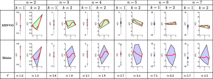
Figure 18: Comparison of the convex hull of the MINVO and Bézier control points for $k=m\in\{1,2\}$ and different $n$. Letting $x(t)$ denote a polynomial of degree $n$, the column with $k=1$ shows the plot of the curve $p(t)=x(t)$, and the blue circles denote the control points. The column with $k=2$ shows the plot of the curve $\boldsymbol{p}(t)=\left[\begin{array}[]{cc}t&x(t)\end{array}\right]^{T}$ (which corresponds to the graph of the polynomial $x(t)$ over $t\in[-1,1]$) and the convex hull of the control points. In the last row, $r$ denotes the ratio of the longitudes $\frac{\text{Long}_{\text{Be}}}{\text{Long}_{\text{MV}}}$ (for $k=1$) or the areas $\frac{\text{Area}_{\text{Be}}}{\text{Area}_{\text{MV}}}$ (for $k=2$) of the convex hulls of the control points. The polynomials $x(t)$ pass through $n+1$ random points in the interval $[-1,1]$.

Appendix E Application of the MINVO basis to surfaces

Similar to any other polynomial basis that is nonnegative and is a partition of unity (i.e., the polynomials in the basis sum up to one), the MINVO basis can be applied to generate polynomial surfaces of degree $(q,r)$ contained in the convex hull of its $(q+1)\cdot(r+1)$ control points. Let us define $\boldsymbol{u}_{q}:=\left[\begin{array}[]{ccc}u^{q}&u^{q-1}\cdots&1\end{array}\right]^{T}$ and let $\boldsymbol{A}_{\text{MV},q}$ denote the matrix $\boldsymbol{A}_{\text{MV}}$ for $n=q$. Analogous definitions apply for $v$, $\boldsymbol{v}_{r}$, and $\boldsymbol{A}_{\text{MV},r}$. Moreover, let $\boldsymbol{V}_{\text{MV},j}\in\mathbb{R}^{(q+1)\times(r+1)}$ contain the coordinate $j\in\{x,y,z\}$ of the control points. The parametric equation of the surface will then be given by:

$$\mathbf{s}(u,v)=\left[\begin{array}[]{c}\left(\boldsymbol{A}_{\text{MV},q}\boldsymbol{u}_{q}\right)^{T}\boldsymbol{V}_{\text{MV},x}\\ \left(\boldsymbol{A}_{\text{MV},q}\boldsymbol{u}_{q}\right)^{T}\boldsymbol{V}_{\text{MV},y}\\ \left(\boldsymbol{A}_{\text{MV},q}\boldsymbol{u}_{q}\right)^{T}\boldsymbol{V}_{\text{MV},z}\end{array}\right]\boldsymbol{A}_{\text{MV},r}\boldsymbol{v}_{r}$$

where $\mathbf{s}(u,v)\in\mathbb{R}^{3}$ and $u,v\in[-1,1]$. An example of the MINVO basis applied to generate different bicubic surfaces (i.e., $q=r=3$) is shown in Figure 19. Note however that, when applied to surfaces, the MINVO basis is not guaranteed to generate always a smaller enclosing polyhedron than, for example, the Bézier basis. An in-depth analysis of the comparison of the volumes produced by the Bézier and MINVO bases when applied to surfaces is out of the scope of this paper, and left as future work.

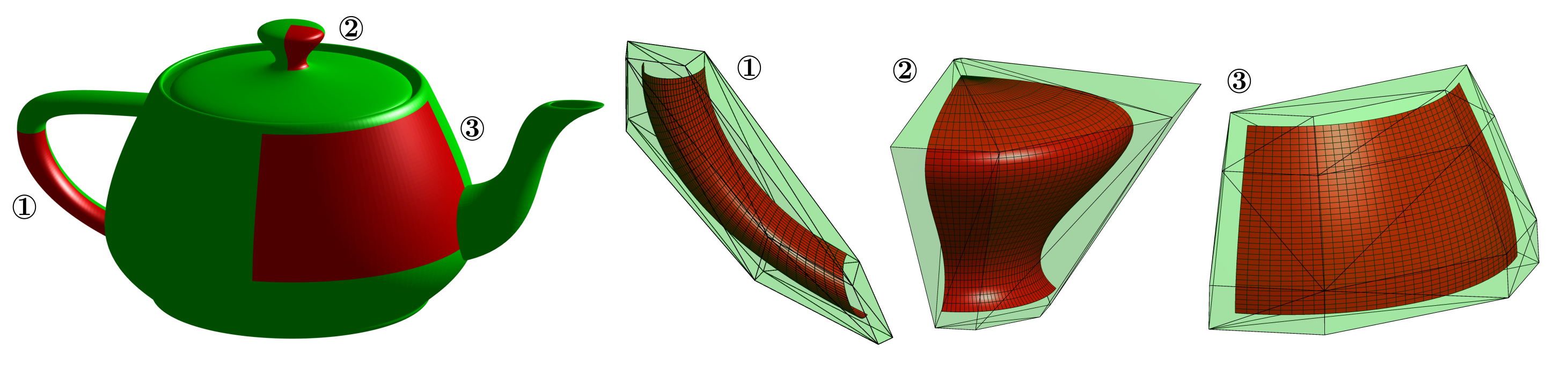
Figure 19: MINVO basis applied to generate outer polyhedra that enclose three bicubic patches of the teapot.

Appendix F Definitions of the union, convex hull, and width of an enclosure (for 2D curves)

Let us define $I:=\{0,1,..,s-1\}$ and $J:=\{0,1,...,h-2\}$, where $s$ denotes the number of subdivisions used, and $h$ is the number of breakpoints per subinterval used in SLEFE. Moreover, let $\mathcal{E}$ denote an enclosure, conv$\left(\cdot\right)$ the convex hull of a set of vertices, $\text{vert}\left(\cdot\right)$ the vertices of an enclosure, and $\text{lssbb}\left(\cdot\right)$ the length of the smallest side of the smallest arbitrarily-oriented bounding box of an enclosure. The union, convex hull, and width are then defined as follows:

	Union	Convex hull	Width
MV/Be	$\bigcup\limits_{i\in I}\mathcal{E}_{i}$	$\text{conv}\left(\bigcup\limits_{i\in I}\text{vert$\left(\mathcal{E}_{i}\right)$}\right)$	$\text{max}\left(\bigcup\limits_{i\in I}\text{lssbb$\left(\mathcal{E}_{i}\right)$}\right)$
SL	$\bigcup\limits_{i\in I,j\in J}\mathcal{E}_{ij}$	$\text{conv}\left(\bigcup\limits_{i\in I,j\in J}\text{vert}\left(\mathcal{E}_{ij}\right)\right)$	$\text{max}\left(\bigcup\limits_{i\in I,j\in J}\text{lssbb}\left(\mathcal{E}_{ij}\right)\right)$

Here, $\mathcal{E}_{i}$ (for MV and Be) is the enclosure of the subinterval $i$, while $\mathcal{E}_{ij}$ (for SL) is the enclosure of the segment $j$ of the subinterval $i$. Note that the area of the union is the sum of the individual areas minus the overlapping area, and it can be computed numerically using [69]. The area of the convex hull is the area of the smallest convex set that contains $\bigcup\limits_{i\in I}\text{vert$\left(\mathcal{E}_{i}\right)$}$ (for MV/Be) or $\bigcup\limits_{i\in I,j\in J}\text{vert}(\mathcal{E}_{ij})$ (for SL), and it can be computed numerically using [70].

Appendix G Comparison with SLEFEs and Bézier: Width

In this section, we compare the MINVO enclosure, Bézier enclosure, and SLEFE in terms of their widths. Given that the width is an important metric for some CAD applications, for this comparison we use data from different real CAD models.

We first use one of the 2D trim curves of the model 10-23022015-110975 from https://traceparts.com. This curve, shown in Fig. 20, is a B-Spline of degree 8, which can be split into 4 Bézier curves. For each of these curves, the comparison between the widths of the enclosures is shown in Table 6.

Figure 20: 2D trim curve of the model 10-23022015-110975 from https://traceparts.com. This curve can be split into four Bézier curves, shown in different colors.

Table 6: Comparison between the width of the MINVO enclosure, Bézier enclosure, and SLEFE for the curve shown in Fig. 20. SL_$h$ denotes the SLEFE computed using $h$ breakpoints per subinterval (i.e., $h-1$ linear segments per subinterval). We use $s=1$ for all the cases of this table.

	Curve 1	Curve 2	Curve 3	Curve 4
$\frac{\text{Width}_{\text{Be}}}{\text{Width}_{\text{MV}}}$	1.05	0.94	0.92	0.96
$\frac{\text{Width}_{\text{SL}_{2}}}{\text{Width}_{\text{MV}}}$	5.95	1.43	1.20	3.92
$\frac{\text{Width}_{\text{SL}_{3}}}{\text{Width}_{\text{MV}}}$	2.20	0.67	1.24	1.62
$\frac{\text{Width}_{\text{SL}_{4}}}{\text{Width}_{\text{MV}}}$	1.12	0.30	0.49	0.79
$\frac{\text{Width}_{\text{SL}_{5}}}{\text{Width}_{\text{MV}}}$	0.58	0.19	0.30	0.47
$\frac{\text{Width}_{\text{SL}_{6}}}{\text{Width}_{\text{MV}}}$	0.37	0.13	0.20	0.30
$\frac{\text{Width}_{\text{SL}_{7}}}{\text{Width}_{\text{MV}}}$	0.22	0.087	0.14	0.20
$\frac{\text{Width}_{\text{SL}_{8}}}{\text{Width}_{\text{MV}}}$	0.16	0.067	0.11	0.15
$\frac{\text{Width}_{\text{SL}_{9}}}{\text{Width}_{\text{MV}}}$	0.13	0.054	0.085	0.12
$\frac{\text{Width}_{\text{SL}_{10}}}{\text{Width}_{\text{MV}}}$	0.097	0.042	0.067	0.090

We then perform a similar analysis using six models taken from the ABC dataset [71], which is an extensive dataset of CAD models. These models are shown in Fig. 21. We obtain the MINVO enclosure, Bézier enclosure, and SLEFE of the 2D (approximate) preimages of ten 3D curves of these models. These 2D curves have degrees ranging from 3 to 9. The results are shown in Fig. 22.

Figure 21: Models taken from the ABC dataset [71].

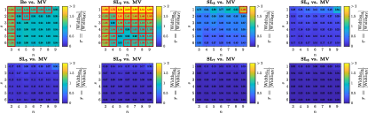
Figure 22: Comparison between the width of the MINVO (MV) enclosure, Bézier (Be) enclosure, and SLEFE (SL) for $n^{\text{th}}$-degree 2D polynomial curves. Here, $s$ is the number of subintervals the curve is divided into, SL_$h$ denotes the SLEFE computed using $h$ breakpoints per subinterval (i.e., $h-1$ linear segments per subinterval), and $[\cdot]$ denotes the mean operator. For every $n$-$s$ combination, a total of 10 polynomial curves obtained from the models shown in Fig. 21 were used. The red squares denote the $n$-$s$ combination for which MINVO achieves a smaller width.

All these previous results (Table 6 and Fig. 22) allow us to conclude that SLEFE performs much better than MINVO in terms of the width of the enclosure. Hence, in applications where it is crucial to have a small width of the enclosure, SLEFE should be preferred over MINVO.

Appendix H Comparison with SLEFEs and Bézier: Area and number of vertices

The $n^{\text{th}}$-degree 2D polynomial curves used pass through $n+1$ points $\left\{\boldsymbol{x}_{0},\ldots,\boldsymbol{x}_{n}\right\}$ that satisfy the dynamical system $\boldsymbol{x}_{k+1}=\boldsymbol{x}_{k}+\text{rand}()-0.15\cdot\boldsymbol{1}$, where $\text{rand}()$ is a random vector in $[0,1]^{2}$ and $\boldsymbol{x}_{0}=\boldsymbol{0}$. Note that these curves are artificially generated, and do not correspond to real CAD data. The results are shown in Figure 23, and some examples are available in Figures 24 and 25.

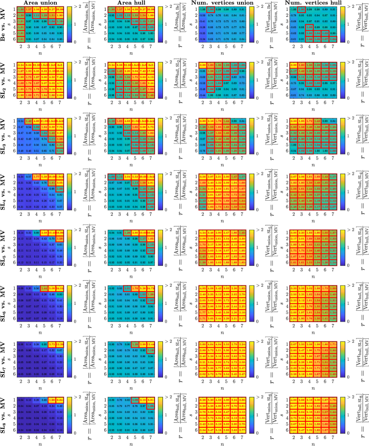
Figure 23: Comparison between the MINVO (MV) enclosure, Bézier (Be) enclosure, and SLEFE (SL) for $n^{\text{th}}$-degree 2D polynomial curves. Here, $s$ is the number of subintervals the curve is divided into, SL_$h$ denotes the SLEFE computed using $h$ breakpoints per subinterval (i.e., $h-1$ linear segments per subinterval), and $[\cdot]$ denotes the mean operator. For every $n$-$s$ combination, a total of 100 polynomial curves obtained as described in H were used. The red squares denote the $n$-$s$ combination for which MINVO achieves a smaller area (first two columns) or fewer number of vertices (last two columns).

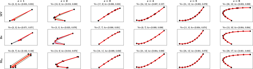
(a) $n=2$

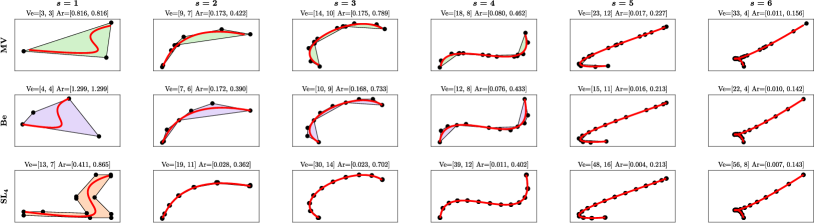
(b) $n=3$

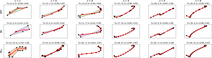
(c) $n=4$

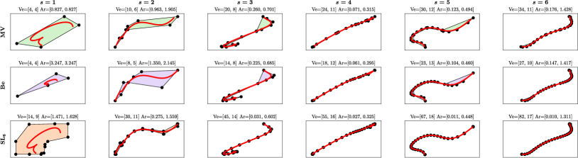
(d) $n=5$

Figure 24: Comparison between the MINVO (MV) enclosure, the Bézier (Be) enclosure, and the SLEFE (SL) for $n^{\text{th}}$-degree 2D polynomial curves obtained as described in H. SL_$h$ denotes the SLEFE computed using $h$ breakpoints per subinterval (i.e., $h-1$ linear segments per subinterval), and $s$ is the number of subdivisions used. In all these plots, $h=n+1$ is used. The notation used is $\text{Ve}=[a,b]$ (where $a$ is the number of vertices of the union and $b$ is the number of vertices of the convex hull) and $\text{Ar}=[c,d]$ (where $c$ is the area of the union of the enclosures and $d$ is the area of the convex hull of the enclosures). The black points are the vertices of the union. Note that this figure shows only some cases that have $h=n+1$, but the results in Fig. 23 include all the cases with different values of $h$, $n$, and $s$.

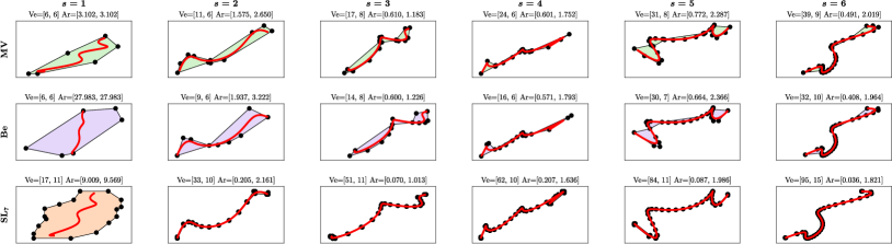
(a) $n=6$

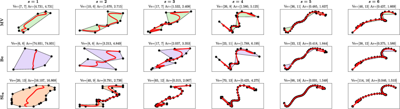
(b) $n=7$

Figure 25: Comparison between the MINVO (MV) enclosure, the Bézier (Be) enclosure, and the SLEFE (SL) for $n^{\text{th}}$-degree 2D polynomial curves obtained as described in H. SL_$h$ denotes the SLEFE computed using $h$ breakpoints per subinterval (i.e., $h-1$ linear segments per subinterval), and $s$ is the number of subdivisions used. In all these plots, $h=n+1$ is used. The notation used is $\text{Ve}=[a,b]$ (where $a$ is the number of vertices of the union and $b$ is the number of vertices of the convex hull) and $\text{Ar}=[c,d]$ (where $c$ is the area of the union of the enclosures and $d$ is the area of the convex hull of the enclosures). The black points are the vertices of the union. Note that this figure shows only some cases that have $h=n+1$, but the results in Fig. 23 include all the cases with different values of $h$, $n$, and $s$.

Appendix I Comparison between MINVO and SLEFE in terms of runtime and simplicity in the implementation

In Section 8 the MINVO enclosure and the SLEFE are compared in terms of enclosing area and number of vertices. The enclosing area is important in terms of conservativeness of the enclosure with respect to the curve, while the number of vertices can have a direct impact on the computation time (for example, in settings where the curve is a decision variable in an optimization problem and there is one constraint per vertex), and on the memory needed to store them.

There are also other applications where the runtime to obtain the enclosure is important. In this section, we compare the runtimes needed to obtain the SLEFE and the MINVO enclosure from a curve given in its Bézier form (i.e., $\boldsymbol{V}_{\text{Be}}$ is given):

• The MINVO enclosure is obtained by simply doing $\boldsymbol{V}_{\text{MV}}=\boldsymbol{V}_{\text{Be}}\boldsymbol{A}_{\text{Be}}\boldsymbol{A}_{\text{MV}}^{-1}$ (Eq. 5), where the term $\boldsymbol{A}_{\text{Be}}\boldsymbol{A}_{\text{MV}}^{-1}$ is tabulated offline using the matrices available in Table 3 and [48] for each degree $n$. If the curve were given instead in its monomial form (i.e., $\boldsymbol{P}$ is given), then the computation of the MINVO enclosure would also be a simple matrix multiplication: $\boldsymbol{V}_{\text{MV}}=\boldsymbol{P}\boldsymbol{A}_{\text{MV}}^{-1}$, where $\boldsymbol{A}_{\text{MV}}^{-1}$ is tabulated offline.

• The SLEFE enclosure is obtained as detailed in [72, Section 3.3], using the tabulated values given by the SubLiME package [73]. We optimize the speed of the SLEFE implementation leveraging vector and matrix operations. Note however that the SLEFE computation requires $\text{max}(\cdot)$ and $\text{min}(\cdot)$ operators, and hence it cannot be obtained as a single matrix multiplication.

The timing results are shown in Table 7. On average, the MINVO enclosure can be obtained $20.4$ times faster than the SLEFE enclosure. These timing results were obtained using Matlab^® R2021b on an AlienWare Aurora r8 desktop running Ubuntu 18.04 and equipped with an Intel^® Core^TM i9-9900K CPU, 3.60GHz$\times$16 and 62.6 GiB.

Table 7: Computation times required to find the MINVO (MV) enclosure and the SLEFE (SL) for $n^{\text{th}}$-degree polynomial curves. SL_$h$ denotes the SLEFE computed using $h$ breakpoints per subinterval (i.e., $h-1$ linear segments per subinterval), $\text{ct}(\cdot)$ denotes the computation time, and $[\cdot]$ denotes the mean operator. For each cell in this table, a total of 30 random polynomials passing through random points in $[-1,1]$ were used. All these cases have $s=1$.

		Degree n
		$\mathbf{2}$	$\mathbf{3}$	$\mathbf{4}$	$\mathbf{5}$	$\mathbf{6}$	$\mathbf{7}$
Ratios of comp. times	$\frac{\left[\text{ct}\left(\text{\text{SL}}_{2}\right)\right]}{\left[\text{ct}(\text{MV})\right]}$	24.8	24.0	20.8	18.3	15.6	13.3
	$\frac{\left[\text{ct}\left(\text{\text{SL}}_{3}\right)\right]}{\left[\text{ct}(\text{MV})\right]}$	24.4	22.8	20.9	18.3	15.6	14.4
	$\frac{\left[\text{ct}\left(\text{\text{SL}}_{4}\right)\right]}{\left[\text{ct}(\text{MV})\right]}$	27.3	24.9	21.0	18.9	16.1	15.1
	$\frac{\left[\text{ct}\left(\text{\text{SL}}_{5}\right)\right]}{\left[\text{ct}(\text{MV})\right]}$	26.4	23.3	20.8	18.6	16.9	15.6
	$\frac{\left[\text{ct}\left(\text{\text{SL}}_{6}\right)\right]}{\left[\text{ct}(\text{MV})\right]}$	26.3	25.0	21.8	19.2	16.8	15.1
	$\frac{\left[\text{ct}\left(\text{\text{SL}}_{7}\right)\right]}{\left[\text{ct}(\text{MV})\right]}$	26.2	24.2	22.3	19.0	17.5	15.6
	$\frac{\left[\text{ct}\left(\text{\text{SL}}_{8}\right)\right]}{\left[\text{ct}(\text{MV})\right]}$	27.8	25.9	22.8	19.8	17.6	15.6

Finally, another aspect that one may consider is the simplicity of the implementation. As detailed above, only a single matrix multiplication is required to obtain the MINVO enclosure, which translates into a simple one line of code in most of the modern programming languages. The SLEFE computation also has a simple implementation, in this case involving sums, multiplications, $\text{max}(\cdot)$, and $\text{min}(\cdot)$ operators. Code examples of how to use MINVO and SLEFE are available at https://github.com/mit-acl/minvo (for both MINVO and SLEFE) and [73] (for SLEFE).

References

- [1] A. Efremov, V. Havran, H.-P. Seidel, Robust and numerically stable Bézier clipping method for ray tracing nurbs surfaces, in: Proceedings of the 21st spring conference on Computer graphics, 2005, pp. 127–135.
- [2] T. W. Sederberg, T. Nishita, Curve intersection using Bézier clipping, Computer-Aided Design 22 (9) (1990) 538–549.
- [3] C. Schulz, Bézier clipping is quadratically convergent, Computer Aided Geometric Design 26 (1) (2009) 61–74.
- [4] E. G. Gilbert, D. W. Johnson, S. S. Keerthi, A fast procedure for computing the distance between complex objects in three-dimensional space, IEEE Journal on Robotics and Automation 4 (2) (1988) 193–203.
- [5] V. Cichella, I. Kaminer, C. Walton, N. Hovakimyan, Optimal motion planning for differentially flat systems using bernstein approximation, IEEE Control Systems Letters 2 (1) (2017) 181–186.
- [6] R. D. Hersch, Font rasterization: the state of the art, From Object Modelling to Advanced Visual Communication (1994) 274–296.
- [7] H. Nguyen, Gpu Gems 3, Addison-Wesley Professional, 2007.
- [8] D. Cardoze, A. Cunha, G. L. Miller, T. Phillips, N. Walkington, A Bézier-based approach to unstructured moving meshes, in: Proceedings of the twentieth annual symposium on Computational geometry, 2004, pp. 310–319.
- [9] S. H. Chuang, W. Lin, Tool-path generation for pockets with freeform curves using Bézier convex hulls, The International Journal of Advanced Manufacturing Technology 13 (2) (1997) 109–115.
- [10] S.-H. F. Chuang, C. Kao, One-sided arc approximation of b-spline curves for interference-free offsetting, Computer-Aided Design 31 (2) (1999) 111–118.
- [11] J. Tordesillas, B. T. Lopez, J. P. How, FASTER: Fast and safe trajectory planner for flights in unknown environments, in: 2019 IEEE/RSJ International Conference on Intelligent Robots and Systems (IROS), IEEE, 2019.
- [12] J. Tordesillas, J. P. How, MADER: Trajectory planner in multiagent and dynamic environments, IEEE Transactions on Robotics (2021).
- [13] J. Tordesillas, J. P. How, PANTHER: Perception-aware trajectory planner in dynamic environments, arXiv preprint arXiv:2103.06372 (2021).
- [14] J. A. Preiss, K. Hausman, G. S. Sukhatme, S. Weiss, Trajectory optimization for self-calibration and navigation., in: Robotics: Science and Systems, 2017.
- [15] O. K. Sahingoz, Generation of Bézier curve-based flyable trajectories for multi-UAV systems with parallel genetic algorithm, Journal of Intelligent & Robotic Systems 74 (1-2) (2014) 499–511.
- [16] W. Ding, W. Gao, K. Wang, S. Shen, Trajectory replanning for quadrotors using kinodynamic search and elastic optimization, in: 2018 IEEE International Conference on Robotics and Automation (ICRA), IEEE, 2018, pp. 7595–7602.
- [17] B. Zhou, F. Gao, L. Wang, C. Liu, S. Shen, Robust and efficient quadrotor trajectory generation for fast autonomous flight, IEEE Robotics and Automation Letters 4 (4) (2019) 3529–3536.
- [18] G. Herron, Polynomial bases for quadratic and cubic polynomials which yield control points with small convex hulls, Computer aided geometric design 6 (1) (1989) 1–9.
- [19] J. Kuti, P. Galambos, P. Baranyi, Minimal volume simplex (mvs) approach for convex hull generation in tp model transformation, in: IEEE 18th International Conference on Intelligent Engineering Systems INES 2014, IEEE, 2014, pp. 187–192.
- [20] J. Li, J. M. Bioucas-Dias, Minimum volume simplex analysis: A fast algorithm to unmix hyperspectral data, in: IGARSS 2008-2008 IEEE International Geoscience and Remote Sensing Symposium, Vol. 3, IEEE, 2008, pp. III–250.
- [21] D. Nairn, J. Peters, D. Lutterkort, Sharp, quantitative bounds on the distance between a polynomial piece and its Bézier control polygon, Computer Aided Geometric Design 16 (7) (1999) 613–631.
- [22] M. I. Karavelas, P. D. Kaklis, K. V. Kostas, Bounding the distance between 2d parametric Bézier curves and their control polygon, Computing 72 (1-2) (2004) 117–128.
- [23] W. Ma, R. Zhang, Efficient piecewise linear approximation of Bézier curves with improved sharp error bound, in: International Conference on Geometric Modeling and Processing, Springer, 2006, pp. 157–174.
- [24] J. Peters, X. Wu, Sleves for planar spline curves, Computer Aided Geometric Design 21 (6) (2004) 615–635.
- [25] C. McCann, Exploring properties of high-degree SLEFEs, Tech. rep., University of Florida (2004).
- [26] D. Lutterkort, J. Peters, Tight linear bounds on the distance between a spline and its b-spline control polygon, Tech. rep., Purdue University (1999).
- [27] D. Lutterkort, J. Peters, Tight linear envelopes for splines, Numerische Mathematik 89 (4) (2001) 735–748.
- [28] A. Kanazawa, On the minimal volume of simplices enclosing a convex body, Archiv der Mathematik 102 (5) (2014) 489–492.
- [29] D. Galicer, M. Merzbacher, D. Pinasco, The minimal volume of simplices containing a convex body, The Journal of Geometric Analysis 29 (1) (2019) 717–732.
- [30] V. Klee, Facet-centroids and volume minimization, Studia Scientiarum Mathematicarum Hungarica 21 (1986) 143–147.
- [31] G. Vegter, C. Yapy, Finding minimal circumscribing simplices part 1: Classifying local minima, Tech. rep., University of Groningen and New York University (1993).
- [32] Y. Zhou, S. Suri, Algorithms for a minimum volume enclosing simplex in three dimensions, SIAM Journal on Computing 31 (5) (2002) 1339–1357.
- [33] T. Uezato, M. Fauvel, N. Dobigeon, Hyperspectral unmixing with spectral variability using adaptive bundles and double sparsity, IEEE Transactions on Geoscience and Remote Sensing 57 (6) (2019) 3980–3992.
- [34] E. M. Hendrix, I. García, J. Plaza, A. Plaza, On the minimum volume simplex enclosure problem for estimating a linear mixing model, Journal of Global Optimization 56 (3) (2013) 957–970.
- [35] D. M. Rogge, B. Rivard, J. Zhang, J. Feng, Iterative spectral unmixing for optimizing per-pixel endmember sets, IEEE Transactions on Geoscience and Remote Sensing 44 (12) (2006) 3725–3736.
- [36] M.-D. Iordache, J. Bioucas-Dias, A. Plaza, Unmixing sparse hyperspectral mixtures, in: 2009 IEEE International Geoscience and Remote Sensing Symposium, Vol. 4, IEEE, 2009, pp. IV–85.
- [37] M. Velez-Reyes, A. Puetz, M. P. Hoke, R. B. Lockwood, S. Rosario, Iterative algorithms for unmixing of hyperspectral imagery, in: Algorithms and Technologies for Multispectral, Hyperspectral, and Ultraspectral Imagery IX, Vol. 5093, International Society for Optics and Photonics, 2003, pp. 418–429.
- [38] K. Ranestad, B. Sturmfels, On the convex hull of a space curve, Advances in Geometry 12 (1) (2012) 157–178.
- [39] V. D. Sedykh, Structure of the convex hull of a space curve, Journal of Soviet Mathematics 33 (4) (1986) 1140–1153.
- [40] D. Derry, Convex hulls of simple space curves, Canadian Journal of Mathematics 8 (1956) 383–388.
- [41] D. Ciripoi, N. Kaihnsa, A. Löhne, B. Sturmfels, Computing convex hulls of trajectories, Revista de la Unión Matemática Argentina 60 (2019) 637–662.
- [42] K. Mazur, Convex hull of and its use for a partial solution to continuous blotto, Ph.D. thesis, New York University (2018).
- [43] C. Carathéodory, Über den Variabilitätsbereich der Koeffizienten von Potenzreihen, die gegebene Werte nicht annehmen, Mathematische Annalen 64 (1) (1907) 95–115.
- [44] E. Steinitz, Bedingt konvergente Reihen und konvexe Systeme, Journal für die reine und angewandte Mathematik (Crelle’s Journal) (143) (1913) 128–176.
- [45] S. Karlin, L. S. Shapley, Geometry of moment spaces, no. 12, American Mathematical Soc., 1953.
- [46] I. J. Schoenberg, Cardinal spline interpolation, SIAM, 1973.
- [47] C. De Boor, A practical guide to splines, Vol. 27, springer-verlag New York, 1978.
- [48] K. Qin, General matrix representations for b-splines, The Visual Computer 16 (3-4) (2000) 177–186.
- [49] Matlab optimization toolbox, the MathWorks, Natick, MA, USA (2020).
- [50] M. Berger, Geometry i, Springer Science & Business Media, 2009.
- [51] K. Hormann, N. Sukumar, Generalized barycentric coordinates in computer graphics and computational mechanics, CRC press, 2017.
- [52] C. Ericson, Real-time collision detection, CRC Press, 2004.
- [53] G. Blekherman, P. A. Parrilo, R. R. Thomas, Semidefinite optimization and convex algebraic geometry, SIAM, 2012.
- [54] G. Szegő, Orthogonal polynomials, Vol. 23, American Mathematical Society, 1939.
- [55] M. G. Krein, D. Louvish, et al., The Markov moment problem and extremal problems, American Mathematical Society, 1977.
- [56] T. Roh, L. Vandenberghe, Discrete transforms, semidefinite programming, and sum-of-squares representations of nonnegative polynomials, SIAM Journal on Optimization 16 (4) (2006) 939–964.
- [57] P. E. Gill, W. Murray, M. A. Saunders, SNOPT: An SQP algorithm for large-scale constrained optimization, SIAM Rev. 47 (2005) 99–131.
- [58] P. E. Gill, W. Murray, M. A. Saunders, E. Wong, User’s guide for SNOPT 7.7: Software for large-scale nonlinear programming, Center for Computational Mathematics Report CCoM 18-1, Department of Mathematics, University of California, San Diego, La Jolla, CA (2018).
- [59] J. Löfberg, Yalmip : A toolbox for modeling and optimization in matlab, in: In Proceedings of the CACSD Conference, Taipei, Taiwan, 2004.
- [60] J. Löfberg, Pre- and post-processing sum-of-squares programs in practice, IEEE Transactions on Automatic Control 54 (5) (2009) 1007–1011.
- [61] J. B. Lasserre, Global optimization with polynomials and the problem of moments, SIAM Journal on Optimization 11 (3) (2001) 796–817.
- [62] J. Löfberg, Envelope approximations for global optimization, https://yalmip.github.io/tutorial/envelopesinbmibnb/ (August 2020).
- [63] M. Sayrafiezadeh, An inductive proof for extremal simplexes, Mathematics Magazine 65 (4) (1992) 252–255.
- [64] D. Lutterkort, J. Peters, Optimized refinable enclosures of multivariate polynomial pieces, Computer Aided Geometric Design 18 (9) (2001) 851–863.
- [65] S. Flöry, Fitting curves and surfaces to point clouds in the presence of obstacles, Comput. Aided Geom. Des. 26 (2) (2009) 192–202.
- [66] J. Selinger, L. Linsen, Efficient curvature-optimized g2-continuous path generation with guaranteed error bound for 3-axis machining, in: 2011 15th International Conference on Information Visualisation, IEEE, 2011, pp. 519–527.
- [67] F. Ahmed Sadeq, S. Assaad Salman, On the volume of a polytope in : Basics, Concepts, Methods, Lambert Academic Publishing, 2012.
- [68] G. M. Ziegler, Lectures on polytopes, Vol. 152, Springer Science & Business Media, 2012.
- [69] Mathworks®, Area of polyshape, https://www.mathworks.com/help/matlab/ref/polyshape.area.html (2022).
- [70] Mathworks®, Convex hull, https://www.mathworks.com/help/matlab/ref/convhull.html (2022).
- [71] S. Koch, A. Matveev, Z. Jiang, F. Williams, A. Artemov, E. Burnaev, M. Alexa, D. Zorin, D. Panozzo, ABC: A big CAD model dataset for geometric deep learning, in: The IEEE Conference on Computer Vision and Pattern Recognition (CVPR), 2019.
- [72] A. Myles, J. Peters, Threading splines through 3d channels, Computer-Aided Design 37 (2) (2005) 139–148.
- [73] X. Wu, J. Peters, The SubLiME (subdividable linear maximum-norm enclosure) package, http://www.cise.ufl.edu/research/SurfLab/download/SubLiME.tar.gz.