New rotating black holes in non-linear Maxwell $f({\cal R})$ gravity

Abstract

We investigate static and rotating charged spherically symmetric solutions in the framework of $f({\cal R})$ gravity, allowing additionally the electromagnetic sector to depart from linearity. Applying a convenient, dual description for the electromagnetic Lagrangian, and using as an example the square-root $f({\cal R})$ correction, we solve analytically the involved field equations. The obtained solutions belong to two branches, one that contains the Kerr-Newman solution of general relativity as a particular limit, and one that arises purely from the gravitational modification with no general-relativity limit. The novel black hole solution has a true central singularity which is hidden behind a horizon, however for particular parameter regions the horizon disappears and the singularity becomes a naked one. Furthermore, we investigate the thermodynamical properties of the solutions, such as the temperature, energy, entropy, heat capacity and Gibbs free energy. We extract the entropy and quasilocal energy positivity conditions, we show that negative-temperature, ultracold, black holes are possible, and we show that the obtained solutions are thermodynamically stable for suitable model parameter regions.

I Introduction

The detection of gravitational waves from the binary black hole and binary neutron star mergers by the LIGO-VIRGO collaboration Abbott et al. (2016, 2017a); Abbott et al. (2017b) opened the new era of multi-messenger astronomy. In this novel window to investigate the universe the central role is played by spherically symmetric compact objects and black holes. Since their properties are determined by the underlying gravitational theory recently there has been an increased interest in studying such solutions in various extensions of general relativity (GR).

The simplest modification of GR arises by generalizing the action through arbitrary functions of the Ricci scalar, resulting to $f({\cal R})$ gravity De Felice and Tsujikawa (2010); Nojiri and Odintsov (2011). Nevertheless, one can build more complicated constructions using higher-order corrections, such as the Gauss-Bonnet term $G$ and its functions Wheeler (1986); Antoniadis et al. (1994); Nojiri and Odintsov (2005); De Felice and Tsujikawa (2009), Lovelock combinations Lovelock (1971); Deruelle and Farina-Busto (1990), Weyl combinations Mannheim and Kazanas (1989), higher spatial-derivatives as in Hořava-Lifshitz gravity Horava (2009), etc. On the other hand, one can be based in the teleparallel formulation of gravity, and construct its modifications such as in $f(T)$ gravity Cai et al. (2016); Bengochea and Ferraro (2009); Linder (2010), in $f(T,T_{G})$ gravity Kofinas and Saridakis (2014), etc. Hence, in all these classes of modified gravity one can extract the spherically symmetric black hole solutions and study their properties Aharony et al. (2000); Awad (2006); Awad and Johnson (2000a, b); Cai et al. (2013); Anabalon et al. (2014); Cisterna and Erices (2014); Babichev et al. (2015); El Hanafy and Nashed (2016); Brihaye et al. (2016); Cisterna et al. (2016); Babichev et al. (2017); Cvetković and Simić (2018); Erices and Martinez (2018); Cisterna et al. (2017, 2018); Gonzalez et al. (2012); Capozziello et al. (2013); Iorio and Saridakis (2012); Nashed (2013a); Aftergood and DeBenedictis (2014); Paliathanasis et al. (2014); Nashed (2015a, b); Junior et al. (2015); Kofinas et al. (2015); Nashed and El Hanafy (2017); Cruz et al. (2017); Awad and Nashed (2017); Ahmed et al. (2016); Farrugia et al. (2016); Koutsoumbas et al. (2018); Mai and Lu (2017); Doneva et al. (2018); Awad et al. (2017); Bejarano et al. (2017); Abdalla et al. (2019); Nashed and Saridakis (2019); Destounis et al. (2019); Papantonopoulos and Vlachos (2020).

In general, the obtained spherically symmetric solutions can be classified either in branches which are extensions of the corresponding GR solutions, coinciding exactly with them in a particular limit, or to novel branches that appear purely from the gravitational modification and do not possess a GR limit. In both cases, the obtained black holes and compact objects present new properties which may be potentially detectable in the gravitational waves arising from mergers. Thus, studying the properties of spherically symmetric solutions in various modified gravities is crucial in order to put the new observational tool of multi-messenger astronomy to work.

It is the aim of the present study to derive new charged black hole solutions in the context of $f({\cal R})$ gravity, allowing additionally for possible non-linearities in the Maxwell sector. The plan of the manuscript is as follows: In Section II, we present a convenient way to handle the possible electrodynamic non-linearities. In Section III we extract static and rotating spherically symmetric black hole solutions and in Section IV we calculate all the thermodynamical quantities such as the entropy, Hawking temperature, heat capacity and Gibb’s free energy, analyzing additionally the stability of the solutions. Finally, Section V is devoted to discussion and conclusions.

II Dual representation of non-linear electrodynamics

In this section we present a new way for the description of non-linear electrodynamics, which is valid independently of the specific electromagnetic Lagrangian and which allows for an easy handling concerning the derivation of field equations. We start with a general gauge-invariant electromagnetic Lagrangian of the form ${\cal L({\cal F})}$, where ${\cal F}=\frac{1}{4}{\cal F}_{\alpha\beta}{\cal F}^{\alpha\beta}$ is the usual anti-symmetric Faraday tensor defined as ${\cal F}_{\alpha\beta}=2{V}_{[\alpha,\beta]},$ with ${V}_{\mu}$ the gauge potential 1-form and where square brackets denote symmetrization Plebański (1970). As usual, linear, Maxwell electrodynamics is obtained for ${\cal L({\cal F})}=4{\cal F}$.

For the purposes of this work we consider a dual representation, introducing the auxiliary field ${\cal P}_{\alpha\beta}$, which has been proven convenient if one desires to embed electromagnetic in the framework of general relativity Ayon-Beato (1999); Salazar I. et al. (1987). In particular, we impose the Legendre transformation

$${\mathbb{H}}=2{\cal F}{\cal L}_{\cal F}-{\cal L},$$ (1)

with ${\cal L}_{\cal F}\equiv\frac{\partial{\cal L}}{\partial{\cal F}}$. Defining

$${\cal P}_{\mu\nu}={\cal L}_{\cal F}{\cal F}_{\mu\nu},$$ (2)

we immediately find that ${\mathbb{H}}$ is an arbitrary function of the invariant

$${\cal P}=\frac{1}{4}{\cal P}_{\alpha\beta}{\cal P}^{\alpha\beta}={\cal L}_{\cal F}^{2}{\cal F}.$$ (3)

Using (1), the Lagrangian of non-linear electrodynamics can be represented in terms of ${\cal P}$ as

$${\cal L}=2{\cal P}{\mathbb{H}}_{\cal P}-{\mathbb{H}},$$ (4)

while

$${\cal F}_{\mu\nu}={\mathbb{H}}_{\cal P}{\cal P}_{\mu\nu},$$ (5)

with ${\mathbb{H}}_{\cal P}=\frac{\partial{\mathbb{H}}}{\partial{\cal P}}$.

The field equations thus acquire the form Ayon-Beato (1999)

$$\partial_{\nu}\left(\sqrt{-g}{\cal P}^{\mu\nu}\right)=0,$$ (6)

and the corresponding energy-momentum tensor is given as

$${{{\mathfrak{T}}^{{}^{{}^{{\!\!\!\!\scriptstyle{nlem}}}}}}}^{\nu}_{\mu}\equiv 2({\mathbb{H}}_{\cal P}{\cal P}_{\mu\alpha}{\cal P}^{\nu\alpha}-\delta_{\mu}^{\nu}[2{\cal P}{\mathbb{H}}_{\cal P}-{\mathbb{H}}]).$$ (7)

We mention that in general (7) has a non-vanishing trace

$${{{\mathfrak{T}}^{{}^{{}^{{\!\!\!\!\scriptstyle{nlem}}}}}}}=8({\mathbb{H}}-{\mathbb{H}}_{\cal P}{\cal P}),$$ (8)

which becomes zero only in the case of the linear theory. Finally, the electric and magnetic fields in spherical coordinates can be calculated as Ayon-Beato (1999); Salazar I. et al. (1987)

$$E=\int{\cal F}_{tr}dr=\int{\mathbb{H}}_{\cal P}{\cal P}_{tr}dr,$$

$$B_{r}=\int{\cal F}_{r\phi}d\phi=\int{\mathbb{H}}_{\cal P}{\cal P}_{r\phi}d\phi,$$

$$B_{\theta}=\int{\cal F}_{\theta r}dr=\int{\mathbb{H}}_{\cal P}{\cal P}_{\theta r}dr,$$

$$B_{\phi}=\int{\cal F}_{\phi r}dr=\int{\mathbb{H}}_{\cal P}{\cal P}_{\phi r}dr.$$ (9)

III Static and rotating black hole solutions in non-linear Maxwell $f({\cal R})$ gravity

In this section we consider non-linear electrodynamics in a gravitational background governed by $f({\cal R})$ gravity, and we extract charged black hole solutions. The total action is written as Carroll et al. (2004)

$$S_{t}=\frac{1}{2\kappa}\int\sqrt{-g}f({\cal R})~{}d^{4}x+\int\sqrt{-g}{\cal L({\cal F})}~{}d^{4}x,$$ (10)

where $\sqrt{-g}$ is the determinant of the metric $g_{\mu\nu}$ and $\kappa$ is the gravitational constant (from now on we set $\kappa=1$ and all quantities are measured in these units). Performing variation with respect to the metric leads to the gravitational field equations Cognola et al. (2005); Koivisto and Kurki-Suonio (2006):

$$\!\!\!\!\!\!\!\!\!\!\!\!\!\!\!\!\xi_{\mu\nu}={\cal R}_{\mu\nu}f_{\cal R}-\frac{1}{2}g_{\mu\nu}f({\cal R})-2g_{\mu\nu}\Lambda+g_{\mu\nu}\Box f_{\cal R}$$

$$-\nabla_{\mu}\nabla_{\nu}f_{\cal R}-8\pi{{{\mathfrak{T}}^{{}^{{}^{{\!\!\!\!\scriptstyle{nlem}}}}}}}_{\mu\nu}\equiv 0,$$ (11)

where $\Box$ is the D’Alembertian operator defined as $\Box=\nabla_{\alpha}\nabla^{\alpha}$, $\nabla_{\alpha}V^{\beta}$ is the covariant derivative of the vector $V^{\beta}$, $f_{\cal R}\equiv\frac{df({\cal R})}{d{\cal R}}$, and the electromagnetic energy-momentum tensor ${{{\mathfrak{T}}^{{}^{{}^{{\!\!\!\!\scriptstyle{nlem}}}}}}}_{\mu\nu}$ is given by (7). Additionally, taking the trace of (III) gives

$$\xi={\cal R}f_{\cal R}-2f({\cal R})-8\Lambda+3\Box f_{\cal R}-{{{\mathfrak{T}}^{{}^{{}^{{\!\!\!\!\scriptstyle{nlem}}}}}}},$$ (12)

with ${{{\mathfrak{T}}^{{}^{{}^{{\!\!\!\!\scriptstyle{nlem}}}}}}}$ given by (8).

III.1 Static solutions

In order to extract black hole solutions we consider a spherically symmetric metric of the form

$$ds^{2}=H(r)dt^{2}-\frac{dr^{2}}{H(r)}-r^{2}(d\theta^{2}+\sin^{2}\theta d\phi^{2}).$$ (13)

Thus, the corresponding Ricci scalar becomes

$${\cal R}=\frac{2-r^{2}H^{\prime\prime}-4rH^{\prime}-2H}{r^{2}},$$ (14)

where from now on primes denote derivatives with respect to $r$. Concerning the electromagnetic potential 1-form we consider the general ansatz Elizalde et al. (2020)

$$V:=q(r)dt+n(\phi)dr+s(r)d\phi,$$ (15)

with $q(r)$,$s(r)$,$n(\phi)$ three free functions reproducing the electric and magnetic charges in the vector potential where ${\cal P}=dV$ and $V=V_{\nu}dx^{\nu}$.

In the following, without loss of generality, and just to provide an example of the method at hand, we focus on the square-root $f({\cal R})$ correction to general relativity, where $f({\cal R})={\cal R}-2\alpha\sqrt{{\cal R}}$ Dimitrijevic et al. (2019); Nashed and Capozziello (2019). Inserting the metric (13) and the potential (15) into the general field equations (III), (12), (6) we obtain the following non-vanishing field equations:

$$\!\!\!\!\!\!\!\!\!\!\!\!\!\!\!\!\xi_{t}{}^{t}=\frac{1}{4r^{6}\sqrt{R^{5}}}\Big{\{}2Rr^{6}HH^{\prime\prime\prime\prime}+3r^{6}HH^{\prime\prime\prime 2}+r^{3}H^{\prime\prime\prime}[r^{2}H^{\prime\prime}(12H-rH^{\prime})-4r^{2}H^{\prime 2}-2r(31H-1)H^{\prime}+48H(1-H)]$$ (16)

$$\ \ \ \ \ \ \ \ \ \ \ \ +2r^{6}H^{\prime\prime 3}+4r^{4}H^{\prime\prime 2}(6rH^{\prime}+15H-4)+2r^{2}H^{\prime\prime}[57r^{2}H^{\prime 2}+14rH^{\prime}(57H-5)+4(5+4H-3H^{2})]$$

$$\ \ \ \ \ \ \ \ \ \ \ \ +200r^{3}H^{\prime 3}+4r^{2}H^{\prime 2}(96H-85)+8rH^{\prime}(H-1)(27H-23)+32(H-1)^{2}(2H-1)\Big{\}}$$

$$-\frac{2rsin^{2}\theta q^{\prime}q^{\prime\prime}(2r^{2}\mathbb{H}-rH^{\prime}+1-H)}{2r^{3}\sin^{2}\theta q^{\prime}q^{\prime\prime}+(s^{\prime}-n_{\phi})[2Hs^{\prime\prime}+(s^{\prime}-n_{\phi})(rH^{\prime}-2H)]}$$

$$-\frac{(s^{\prime}\!-\!n_{\phi})\{2rHs^{\prime\prime}(1\!-\!rH^{\prime}\!-\!H-\mathbb{H}r^{2})-(s^{\prime}\!-\!n_{\phi})[r^{2}H^{\prime 2}\!-\!r(1\!+\!H+2r^{2}\mathbb{H})]+2H(H\!-\!1\!-\!r^{3}\mathbb{H}^{\prime}\!-\!r^{2}\mathbb{H})\}}{2r^{2}[2rHs^{\prime\prime}(s^{\prime}-n_{\phi})+2r^{3}\sin^{2}\theta q^{\prime}q^{\prime\prime}+(s^{\prime}-n_{\phi})^{2}(rH^{\prime}-2H)]}=0,$$

$$\!\!\!\!\!\!\!\!\!\!\!\!\!\!\!\!\xi_{t}{}^{\phi}=\frac{4rH\mathbb{H}^{\prime}q^{\prime}(s^{\prime}-n_{\phi})}{2r^{3}\sin^{2}\theta q^{\prime}q^{\prime\prime}+(s^{\prime}-n_{\phi})[2Hs^{\prime\prime}+(s^{\prime}-n_{\phi})(rH^{\prime}-2H)]}=0,\ \ \ \ \ \ \ \ \ \ \ \ \ \ \ \ \ \ \ \ \ \ \ \ \ \ \ \ \ \ \ \ \ \ \ \ \ \ \ \ \ \ \ \ \ \ \ \ \ \ \ \ \ \ \ \ \ \ \ \$$ (17)

$$\!\!\!\!\!\!\!\!\!\!\!\!\!\!\!\!\!\!\!\!\!\!\!\!\xi_{r}{}^{r}=\frac{1}{4r^{4}\sqrt{R^{3}}}\Big{\{}4r^{2}\sqrt{R^{3}}(2r^{2}\mathbb{H}-rH^{\prime}-H+1)+\alpha\Big{[}r^{3}H^{\prime\prime\prime}(rH^{\prime}+4H)-2r^{4}H^{\prime\prime 2}+4r^{2}H^{\prime\prime}[(3+H)-4rH^{\prime}]$$

$$\ \ \ \ \ \ \ \ \ \ \ \ \ \ \ \ \ \ \ \ \ \ \ \ \ \ \ \ \ \ \ \ \ \ \ \ \ \ \ \ \ \ \ \ \ \ \ \ \ \ \ \ \ \ \ \ -50r^{2}H^{\prime 2}+4rH^{\prime}(15-17H)-16(1+2H^{2}-3H)\Big{]}\Big{\}}=0,$$ (18)

$$\!\!\!\!\!\!\!\!\!\!\!\!\!\!\!\xi_{\theta}{}^{\theta}=\frac{1}{4r^{6}\sqrt{R^{5}}\{2r^{3}\sin^{2}\theta q^{\prime}q^{\prime\prime}-(s^{\prime}-n_{\phi})[2Hs^{\prime\prime}+(s^{\prime}-n_{\phi})(rH^{\prime}-2H)]\}}$$

$$\cdot\Big{\{}r^{5}\sqrt{R^{5}}\Big{\{}rH^{\prime\prime}\{2r^{3}\sin^{2}\theta q^{\prime}q^{\prime\prime}-(s^{\prime}-n_{\phi})[2Hs^{\prime\prime}+(s^{\prime}-n_{\phi})(rH^{\prime}-2H)]\}-\frac{1}{2}rH^{\prime 2}(s^{\prime}-n_{\phi})^{2}-2r^{4}\mathbb{H}^{\prime}q^{\prime 2}\sin^{2}\theta$$

$$\ \ \ \ \ \ \ \ \ \ \ \ \ -[q^{\prime}q^{\prime\prime}r^{3}\sin^{2}\theta-2rHs^{\prime\prime}(s^{\prime}-n_{\phi})](2r\mathbb{H}-H^{\prime})-(H+r^{2}\mathbb{H})[(s^{\prime}-n_{\phi})^{2}-2rH(\phi^{\prime 2}-2s^{\prime}n_{\phi}+s^{\prime 2})]\Big{\}}$$

$$\ \ -\alpha\{2r^{3}\sin^{2}\theta q^{\prime}q^{\prime\prime}-(s^{\prime}-n_{\phi})[2Hs^{\prime\prime}+(s^{\prime}-n_{\phi})(rH^{\prime}-2H)]\}$$

$$\ \,\cdot\Big{\{}2r^{6}RHH^{\prime\prime\prime\prime}-3r^{6}HH^{\prime\prime\prime 2}+2r^{3}H^{\prime\prime\prime}[r^{2}H^{\prime\prime}(rH^{\prime}-7H)+4r^{2}H^{\prime 2}+2rH^{\prime}(14H-1)-22H(1-H)]$$

$$\ \ \ \ \,-4r^{4}[r^{2}H^{\prime\prime 3}+H^{\prime\prime 2}(18H+9rH^{\prime}-5)]-4r^{2}H^{\prime\prime}[33r^{2}H^{\prime 2}+rH^{\prime}(27H-34)+10H+8-18H^{2}]$$

$$\ \ \ \ \,-208r^{3}H^{\prime 3}-4r^{2}H^{\prime 2}(81H-74)+8r(15H-16)(1-H)+16(1-4H+5H^{2}-2H^{3})\Big{\}}\Big{\}}\equiv 0,$$ (19)

$$\!\!\!\!\!\!\!\!\!\!\!\!\!\!\!\ \xi_{\phi}{}^{\phi}=\frac{1}{4r^{6}\sqrt{R^{5}}\{2r^{3}\sin^{2}\theta q^{\prime}q^{\prime\prime}-(s^{\prime}-n_{\phi})[2Hs^{\prime\prime}+(s^{\prime}-n_{\phi})(rH^{\prime}-2H)]\}}$$

$$\ \ \cdot\Big{\{}2r^{5}\sqrt{R^{5}}\Big{\{}rH^{\prime\prime}\{2r^{3}\sin^{2}\theta q^{\prime}q^{\prime\prime}-(s^{\prime}-n_{\phi})[2Hs^{\prime\prime}+(s^{\prime}-n_{\phi})(rH^{\prime}-2H)]\}-[rH^{\prime 2}/2-(H+r^{2}\mathbb{H})](s^{\prime}-n_{\phi})^{2}$$

$$\ \ \ \ \ \ \ \ \ \ \ \ \ \ \ \ \ -r[q^{\prime}q^{\prime\prime}r^{2}\sin^{2}\theta+2Hs^{\prime\prime}(s^{\prime}-n_{\phi})](2r\mathbb{H}-H^{\prime})-2r[H\mathbb{H}(\phi^{\prime 2}-2s^{\prime}n_{\phi}+s^{\prime 2})-r^{3}\mathbb{H}^{\prime}q^{\prime 2}\sin^{2}\theta]\Big{\}}$$

$$\ \ \ \ \ +\alpha\{2r^{3}\sin^{2}\theta q^{\prime}q^{\prime\prime}-(s^{\prime}-n_{\phi})[2Hs^{\prime\prime}+(s^{\prime}-n_{\phi})(rH^{\prime}-2H)]\}$$

$$\ \ \ \ \ \,\cdot\Big{\{}2r^{6}RHH^{\prime\prime\prime\prime}+3r^{6}HH^{\prime\prime\prime 2}-2r^{3}H^{\prime\prime\prime}[r^{2}H^{\prime\prime}(rH^{\prime}-7H)+4r^{2}H^{\prime 2}+2rH^{\prime}(14H-1)-22H(1-H)]$$

$$\ \ \ \ \ \ \ \ +4r^{4}[r^{2}H^{\prime\prime 3}+H^{\prime\prime 2}(18H+9rH^{\prime}-5)]+4r^{2}H^{\prime\prime}[33r^{2}H^{\prime 2}+rH^{\prime}(27H-34)+10H+8-18H^{2}]$$

$$\ \ \ \ \ \ \ \ +208r^{3}H^{\prime 3}+4r^{2}H^{\prime 2}(81H-74)-8rH^{\prime}(15H-16)(1-H)-16(1-4H+5H^{2}-2H^{3})\Big{\}}\Big{\}}\equiv 0,$$ (20)

$$\!\!\!\!\!\!\!\!\!\!\!\!\!\!\!\!\!\!\!\!\!\!\!\!\!\!\!\!\!\!\!\!\!\!\!\!\!\!\!\!\!\!\!\!\!\!\!\!\!\!\!\!\!\!\!\!\!\!\!\!\!\!\!\!\!\!\!\!\!\!\xi_{\phi}{}^{t}=\frac{4r^{3}\mathbb{H}^{\prime}\sin^{2}\theta q^{\prime}(s^{\prime}-n_{\phi})}{2rHs^{\prime\prime}(s^{\prime}-n_{\phi})-2r^{3}\sin^{2}\theta q^{\prime}q^{\prime\prime}+(s^{\prime}-n_{\phi})^{2}(rH^{\prime}-2H)}.\ \ \ \ \ \ \ \ \ \ \ \ \ \ \ \ \ \ \ \ \ \ \ \ \ \ \ \ \ \ \ \ \ \ \ \$$ (21)

Finally, the trace equation (12) becomes

$$\!\!\!\!\!\!\!\!\!\!\!\!\!\!\!\xi=\frac{1}{2r^{6}\sqrt{R^{5}}\{2r^{3}\sin^{2}\theta q^{\prime}q^{\prime\prime}-(s^{\prime}-n_{\phi})[2Hs^{\prime\prime}+(s^{\prime}-n_{\phi})(rH^{\prime}-2H)]\}}$$

$$\!\!\!\!\!\cdot\Big{\{}r^{4}\sqrt{R^{5}}\Big{\{}r^{2}H^{\prime\prime}\{2r^{3}\sin^{2}\theta q^{\prime}q^{\prime\prime}-(s^{\prime}-n_{\phi})[2rHs^{\prime\prime}+(s^{\prime}-n_{\phi})(rH^{\prime}-2H)]\}+4r^{5}\mathbb{H}^{\prime}q^{\prime 2}\sin^{2}\theta$$

$$\ \ \ \ \ \ \ \ \ \ \ -r(1+4r^{2}\mathbb{H}-2rH^{\prime}-H)[2q^{\prime}q^{\prime\prime}r^{2}\sin^{2}\theta-2Hs^{\prime\prime}(s^{\prime}-n_{\phi})]-[2r^{2}H^{\prime 2}-r(3H+4r^{2}\mathbb{H}+1)](s^{\prime}-n_{\phi})^{2}$$

$$\ \ \ \ \ \ \ \ \ \ \ -2H[\phi^{\prime 2}-2s^{\prime}n_{\phi}+s^{\prime 2}](1+2r^{3}\mathbb{H}^{\prime}-H+4r^{2}H)\Big{\}}$$

$$+\alpha\{2r^{3}\sin^{2}\theta q^{\prime}q^{\prime\prime}-(s^{\prime}-n_{\phi})[2Hs^{\prime\prime}+(s^{\prime}-n_{\phi})(rH^{\prime}-2H)]\}$$

$$\cdot\Big{\{}2r^{6}RHH^{\prime\prime\prime\prime}+3r^{6}HH^{\prime\prime\prime 2}-2r^{3}H^{\prime\prime\prime}[r^{2}H^{\prime\prime}(rH^{\prime}-6H)+4r^{2}H^{\prime 2}+2rH^{\prime}(16H-1)-24H(1-H)]$$

$$\ \,\ +4r^{6}H^{\prime\prime 3}+2r^{4}H^{\prime\prime 2}(3-17H-5rH^{\prime})-4r^{2}H^{\prime\prime}[41r^{2}H^{\prime 2}-2rH^{\prime}(16H^{\prime}-23)+4(H+3-4H^{2})]$$

$$\ \ \,-136r^{3}H^{\prime 3}+2r^{2}H^{\prime 2}(106-117H)+8rH^{\prime}(15H-13)(1-H)-16(2H-1)(1-H)^{2}\Big{\}}\Big{\}}\equiv 0.$$ (22)

From Eqs. (17) and (21) we acquire

$$s(r)=c_{4}r,\quad n(\phi)=c_{4}\phi.$$ (23)

Inserting (23) into Eqs. (III.1) and (III.1) it is easy to show that two of the other equations coincide, namely $\xi_{\theta}{}^{\theta}=\xi_{\phi}{}^{\phi}$. Therefore, the system of differential equations (16), (III.1), (III.1) and (III.1)reduces to three differential equations of three unknowns, $H(r)$, $\mathbb{H}$ and $q(r)$, which can be solved to give the following analytical solutions:

$$\!\!\!\!\!\!-H(r)=\frac{c}{2}+\frac{c_{1}}{r}+\frac{c_{2}}{r^{2}}\,,\qquad\qquad q(r)=\frac{c_{3}}{r}\,,$$

$$\!\!\!\!\!\!\mathbb{H}(r)=\frac{\alpha[3c_{2}+4(c-1)r]r^{2}+\sqrt{2-c}[(c-2)r^{2}-2c_{1}]}{4\sqrt{2-c}r^{4}}\,,$$

(24)

$$\!\!\!\!\!\!-H(r)=\frac{c}{2}-\frac{1}{3\alpha r}-\frac{1}{3\alpha r^{2}}\,,\qquad\qquad q(r)=\frac{c_{3}}{r}\,,$$

$$\!\!\!\!\!\!\mathbb{H}(r)=\frac{\alpha[-3+12(c-1)r]r^{2}+\sqrt{2-c}[3\alpha(c-2)r^{2}+2]}{12\sqrt{2-c}r^{4}}\,.$$

(25)

We stress that we adjust the constants $c_{1}$ and $c_{2}$ so that solutions (III.1) and (III.1) satisfy the trace Eq. (22) too, and hence the whole solution structure is consistent. Additionally, concerning the parameter $c$ we deduce that it must be non-negative in order to maintain the metric signature and also the value 0 is excluded too in order to obtain asymptotic flat spacetime at $r\rightarrow\infty$. If $\alpha=0$ then solution (III.1) holds for any $0<c$ while solution (III.1) does not exist, nevertheless if $\alpha\neq 0$ then we should restrict $c$ to $0<c<2$ in both solutions in order to acquire real ${\mathbb{H}(r)}$.

Concerning the function ${\cal P}$ we find ${\cal P}(r)=\frac{c_{3}^{2}}{2r^{4}}$. Hence, knowing $\mathbb{H}(r)$ we can find that

$$\!\!\!\!\!\!\!\!\!\!\!\!\!\!\!\!\!\!\mathbb{H}({\cal P})=\frac{{\cal P}}{4c_{3}^{2}}\left\{-4c_{1}+\sqrt{2}(c-2)c_{3}{\cal P}^{-1/2}\right.$$

$$\!\!\!\!\!\!\!\!\!\!\!\!\!\!\left.+\alpha c_{3}[{\cal P}(1\!-\!c/2)]^{-1/2}\!\left[3c_{2}\!+\!2^{7/4}(c\!-\!1)\sqrt{c_{3}}{\cal P}^{-1/4}\right]\!\right\}.$$ (26)

Therefore, knowing from (1) that ${\mathbb{H}}=2{\cal F}{\cal L}_{\cal F}-{\cal L}$ and from (3) that ${\cal P}={\cal L}_{\cal F}^{2}{\cal F}$, we can re-write (III.1) as

$$\!\!\!\!\!\!\!\!\!\!\!\!\!\!\!\!\!\!\!\!2{\cal F}{\cal L}_{\cal F}-{\cal L}=\frac{{\cal L}_{\cal F}^{2}{\cal F}}{4c_{3}^{2}}\left\{-4c_{1}+\sqrt{2}(c-2)c_{3}{\cal L}_{\cal F}^{-1}{\cal F}^{-1/2}\right.$$ (27)

$$\ \ \ \ \ \ \left.+\alpha c_{3}{\cal L}_{\cal F}^{-1}[{\cal F}(1-c/2)]^{-1/2}\right.$$

$$\ \ \ \ \ \ \left.\cdot\left[3c_{2}+2^{7/4}(c-1)\sqrt{c_{3}}{\cal L}_{\cal F}^{-1/2}{\cal F}^{-1/4}\right]\right\},$$

which is a differential equation for ${\cal L}({\cal F})$.

According to the value of $c$ the solution of the above differential equation will give a corresponding correction to the standard electromagnetic Lagrangian. Since for our novel solution we have $0<c<2$, in the rest of the work we focus on the case $c=1$, since this leads to the simple solution (but still a novel solution comparing to general relativity)

$${\cal L}({\cal F})=\frac{c_{3}^{2}}{c_{1}}{\cal F}+\frac{c_{3}}{\sqrt{c_{1}}}\sqrt{{\cal F}}c_{4}+c_{1}c_{4}^{2}.$$ (28)

As one can see, the first term is standard linear electromagnetism, while the second term is the non-linear correction of a square-root form. In the general $c$ case the correction terms take more complicated forms.

Let us analyze the properties of the obtained spherically symmetric solutions (III.1), (III.1). These can be re-written in the standard form as

$$ds_{1}{}^{2}=-\left(\frac{c}{2}-\frac{2M}{r}+\frac{q^{2}}{r^{2}}\right)dt^{2}$$

$$\ \ \ \ \ \ \ \ \ \,+\frac{dr^{2}}{\left(\frac{c}{2}-\frac{2M}{r}+\frac{q^{2}}{r^{2}}\right)}+r^{2}d\Omega^{2}\;,$$

$$\textrm{where}\qquad M=-\frac{c_{1}}{2},\qquad q=\sqrt{c_{2}},$$ (29)

for (III.1), and

$$ds_{2}{}^{2}=-\left(\frac{c}{2}-\frac{2M}{r}+\frac{q^{2}}{r^{2}}\right)dt^{2}$$

$$\ \ \ \ \ \ \ \ \ \,+\frac{dr^{2}}{\left(\frac{c}{2}-\frac{2M}{r}+\frac{q^{2}}{r^{2}}\right)}+r^{2}d\Omega^{2}\;,$$

$$\textrm{where}\qquad M=\frac{1}{6\alpha},\qquad q=\frac{1}{\sqrt{6\alpha}},$$ (30)

for (III.1). The first solution branch includes the GR solution in the limit $\alpha\rightarrow 0$ and $c\rightarrow 2$ (solution (III.1) is the generalization of those obtained in Sebastiani and Zerbini (2011) in the static and non-charged case, see also Nashed (2013a); Gamal (2012); Nashed (2014, 2013b)). On the other hand, the second branch exists only in the case $\alpha\neq 0$, and thus it is a novel solution that arises from the $f({\cal R})$ gravitational modification as well as from the electrodynamic non–linearity. Hence, the two solutions, although looking similar, they are fundamentally different, and the fact that the mass of solution (III.1) depends only on $1/\alpha$ is a reflection of the novelty of the solution (such a connection between the gravitational modification parameters with the black hole quantities, in specific exact solutions, is known to be the case in many modified gravity theories). In this work we are interesting in solution (III.1), i.e (III.1), exactly because it is a novel one with no general relativity limit.

In order to investigate the horizons and singularities of the above solutions we calculate the Kretschmann, the Ricci tensor square and the Ricci invariants. For (III.1) we find

$$\!\!\!\!\!\!{\cal R}^{\mu\nu\lambda\rho}{\cal R}_{\mu\nu\lambda\rho}=r^{-8}\Big{\{}8c_{1}(7c_{1}-r^{2})+4c_{1}r(12c_{2}+cr)$$

$$\ \ \ \ \ +cr^{4}(c-4)+4c_{2}r^{2}(3c_{2}-2r)+4r^{3}(r+c_{2}c)\Big{\}},$$

$$\!\!\!\!\!\!{\cal R}^{\mu\nu}{\cal R}_{\mu\nu}=\frac{8c_{1}(c_{1}+r^{2})+cr^{2}(cr^{2}-4c_{1})+4r^{4}(1-c)}{18\alpha^{2}r^{8}},$$

$$\!\!\!\!\!\!{\cal R}=\frac{2-c}{r^{2}},$$

while for (III.1) we acquire

$$\!\!\!\!\!\!\!\!\!-{\cal R}^{\mu\nu\lambda\rho}{\cal R}_{\mu\nu\lambda\rho}=(9\alpha^{2}r^{8})^{-1}\Big{\{}56+9r^{4}\alpha^{2}[c-2]^{2}$$

$$\ \ \ \ \ \ \ \ \ \ -12\alpha r^{3}(c-2)-12r^{2}[\alpha(c-2)-1]+48r\Big{\}},$$

$$\!\!\!\!\!\!\!\!\!{\cal R}^{\mu\nu}{\cal R}_{\mu\nu}=\frac{9r^{4}\alpha^{2}(c-2)^{2}+12\alpha r^{2}(c-2)+8}{18\alpha^{2}r^{8}},$$

$$\!\!\!\!\!\!\!\!\!{\cal R}=\frac{2-c}{r^{2}}.$$ (32)

Expressions (III.1), (32) reveal that the spherically symmetric solutions exhibit a true singularity at $r=0$. Although in the GR case this singularity is always hidden by a horizon, when the $f({\cal R})$ correction is switched on this is not always the case, namely a naked singularity may appear. This issue will be investigated in the next section.

Lastly, concerning the electric and magnetic charges, expressions (II) give

$$\!\!\!\!\!\!\!E=\frac{[(c\!-\!2)r^{2}-8m]\sqrt{2\!-\!c}+r^{2}\alpha[(c\!-\!1)r\!+\!3q^{2}]}{4c_{3}r\sqrt{2\!-\!c}},$$

$$\!\!\!\!\!\!\!B_{\phi}=\frac{c_{4}r([2(c\!-\!2)r^{2}+16m]\sqrt{2\!-\!c}+3r^{2}\alpha[(c\!-\!1)\!+\!2q^{2}])}{24c_{3}{}^{2}\sqrt{2\!-\!c}},$$

$$\!\!\!\!\!\!\!B_{r}=\frac{c_{4}\phi([(c\!-\!2)r^{2}+8m]\sqrt{2\!-\!c}+r^{2}\alpha[2(c\!-\!1)\!+\!3q^{2}])}{4c_{3}{}^{2}\sqrt{2\!-\!c}},$$

while $B_{\theta}=0$. Equation (III.1) shows in a clear way that when the constant $c_{4}=0$ we have no magnetic fields, namely the magnetic fields are related to the integration constant $c_{4}$.

III.2 Rotating solutions

In this subsection we derive rotating solutions that satisfy the field equations (III), (12) and (6). In order to achieve this we apply the following transformation Lemos (1995); Awad (2003):

$$\bar{\phi}=\Xi~{}{\phi}+\omega~{}t,$$

$$\bar{t}=\Xi~{}t+\omega~{}\phi,$$ (34)

with $\omega$ being the rotation parameter and $\Xi=\sqrt{1+\omega^{2}}$. Applying (III.2) to the metric (13) we obtain

$$\!\!\!\!\!\!\!\!\!\!\!\!\!\!\!\!\!ds^{2}=[\Xi^{2}H(r)-\omega^{2}r^{2}\sin^{2}\theta]dt^{2}-\frac{dr^{2}}{H(r)}-r^{2}d\theta^{2}$$

$$\!\!\!\!\!\!\!\!\!\!\!\!\!-[\Xi^{2}r^{2}\sin^{2}\theta\!-\!\omega^{2}H]d\phi^{2}+2\omega\Xi[H\!-\!r^{2}\sin^{2}\theta]dtd\phi,$$ (35)

where $H(r)$ is given by the previously extracted static solutions (III.1), (III.1), and $0\leq r<\infty$, $-\infty<t<\infty$, $0\leq\phi<2\pi$. We mention that the static configuration (13) can be recovered as a special case of the above general metric, if the rotation parameter $\omega$ is set to zero. Hence, for the general gauge potential (15) we acquire the form

$$\bar{V}=\left[\Xi q(r)+\omega s(r)\right]d\bar{t}+n(\phi)dr+\left[\omega q(r)+\Xi s(r)\right]d\bar{\phi}.$$ (36)

Note here that although the transformation (III.2) leaves the local properties of spacetime unaltered, it does change them globally as has been shown in Lemos (1995), since it mixes compact and noncompact coordinates. Thus, the two metrics (13) and (III.2) can be locally mapped into each other but not globally Lemos (1995); Awad (2003).

To conclude, we have succeeded to derive new rotating charged black hole solutions in $f({\cal R})$ gravity, using as a specific example the case $f({\cal R})={\cal R}-2\alpha\sqrt{{\cal R}}$. Similarly to the static case, these belong to two branches, one that contains the Kerr-Newman metric, namely the rotating charged black hole solution of general relativity, as a particular limit (the one arising inserting (III.1) into (III.2)) and one that arises purely from the gravitational modification and does not recover the general relativity solution (the one arising inserting (III.1) into (III.2)). Concerning the singularity properties, as is clear from (III.2), these will be the same with the static solution (13). Therefore, at $r=0$ we obtain a true singularity, and close to $r=0$ the behavior of the invariants are $(K,R_{\mu\nu}R^{\mu\nu})\sim{r^{-8}}$ and $(R)\sim{r^{-2}}$.

IV Thermodynamics

In this section we focus on the investigation of the thermodynamic properties of the obtained black hole solutions. Since solution (III.1) contains the general relativity result, in the following analysis we focus on the novel solution (III.1) that arises solely from the gravitational modification Elizalde et al. (2020); Nashed et al. (2020); Nashed and Capozziello (2019).

We start by introducing the Hawking temperature as Sheykhi (2012, 2010); Hendi et al. (2010); Sheykhi et al. (2010)

$$T_{h}=\frac{H^{\prime}(r_{h})}{4\pi},$$ (37)

where the event horizon is located at $r=r_{h}$ which represents the largest positive root of $H(r_{h})=0$ that satisfies $H^{\prime}(r_{h})\neq 0$. The Bekenstein-Hawking entropy of $f({\cal R})$ gravitational theory is given by Cognola et al. (2011); Zheng and Yang (2018)

$$S(r_{h})=\frac{1}{4}Af_{R}(r_{h}),$$ (38)

with $A$ being the area of the event horizon. Additionally, the quasilocal energy in $f({\cal R})$ gravity is defined as Cognola et al. (2011); Zheng and Yang (2018)

$$\!\!\!\!\!\!\!\!\!\!\!\!\!\!\!\!\!\!\!\!\!\!\!E(r_{h})=\frac{1}{4}\int dr_{h}\Big{[}r_{h}{}^{2}\Big{\{}f(R(r_{h}))-R(r_{h})f_{R}(r_{h})\Big{\}}$$

$$\ \ \ \ \ \ \ \ \ \ \ \ +2f_{R}(r_{h})\Big{]}.$$ (39)

Finally, we can express the black hole mass as a function of the horizon $r_{h}$ and the charge $q$, which for the case (III.1),(III.1) becomes

$${M_{h}}=\frac{r_{h}}{2}\left[\frac{c}{2}+\frac{q^{2}}{r_{h}{}^{2}}\right].$$ (40)

The relation between the metric function $H(r)$ and the radial coordinate $r$ is presented in Fig. 1, which shows the possible horizons of the solution. Note that since in this work for simplicity we are using natural units, in order to be closer to physical cases we should have taken much larger values of $M$ and $q$ and then the radial distance would take much larger values too while $\alpha$ would take much smaller values. However, since in mathematical terms the physical properties of the solutions do not depend on the scale, and in order to avoid graphs with very large/small numbers, we prefer to remain in these representative numbers of order one since they are adequate in order to provide the physical features of the solution.

Moreover, the relation between $M_{h}$ and the horizon radius is depicted in Fig. 2. As one can see, there is a limiting horizon radius after which there is no horizon and the black hole singularity will be a naked singularities. This “degenerate horizon” value $r_{dg}$ can thus be calculated by the condition $\frac{\partial M_{h}}{\partial r_{h}}$= 0, which for solution (III.1),(III.1) yields

$$r_{dg}=\frac{\sqrt{2}q}{\sqrt{c}}.$$

Hence, as we can see, the cosmic censorship theorem can be violated in non-linear Maxwell $f({\cal R})$ gravity.

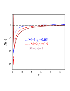
Figure 1: The metric function $H(r)$ vs the radial coordinate $r$, for solution (III.1) with $c=1$, for various mass and charge choices. The black hole horizon is determined by the condition $H(r)=0$. The “degenerate horizon” $r_{dg}$ marks the limiting value after which there is no horizon and the central singularity becomes a naked one (see text).

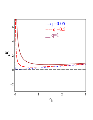
Figure 2: The black hole mass as a function of the horizon $r_{h}$, for solution (III.1) with $c=1$, for various charge choices.

Concerning the Hawking temperature (37), calculating it using the black hole solution (III.1) we find

$${T_{h}}=\frac{cr_{h}{}^{2}-2q^{2}}{8\pi r_{h}{}^{3}}.$$ (41)

We mention that $T_{h}$ does not depend directly on the gravitational modification parameter $\alpha$ (although it indirectly does since the latter affects the horizon). In Fig. 3 we depict the temperature behavior as a function of the horizon. As we observe, for suitable parameter values this can be negative, and according to (41) this happens when $c<\frac{2q^{2}}{r_{h}{}^{2}}$. This implies a formation of an ultracold black hole Davies (1977); Babichev et al. (2013), which reveals the capabilities of the scenario at hand.

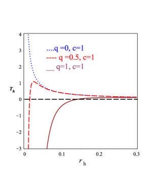
Figure 3: The black hole temperature (41) as a function of the horizon $r_{h}$, for solution (III.1), for solution (III.1) with $c=1$, for various charge choices.

As a next step, using expression (38) the entropy of the black hole (III.1) is calculated as

$${S_{h}}=\frac{\pi r_{h}{}^{2}(\sqrt{2-c}-\alpha r_{h})}{\sqrt{2-c}}.$$ (42)

In Fig. 4 we show the behavior of the entropy as a function of the horizon. Hence, by imposing the entropy positivity condition we obtain

$$\alpha<\frac{\sqrt{c-2}}{r_{h}}.$$

This is one of the main results of the present work, and shows that the gravitational correction of $f({\cal R})$ gravity must be suitably small in order to avoid non-physical black hole properties (see also the discussion in Cvetic et al. (2002); Nojiri et al. (2001); Nojiri and Odintsov (2002, 2017); Clunan et al. (2004); Nojiri et al. (2002) for the entropy negativity in various theories of modified gravity).

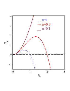
Figure 4: The black hole entropy (42) as a function of the horizon $r_{h}$, for solution (III.1), for various choices of the gravitational modification parameter $\alpha$.

Similarly, using expression (IV) we find the quasilocal energy of the black hole (III.1) as

$${E_{h}}=\frac{r_{h}(4\sqrt{2-c}+4r_{h}\alpha-3r_{h}c\alpha)}{8\sqrt{2-c}}.$$ (43)

From (43) we conclude that in order to have a positive value of the quasilocal energy we must have

$$\!\!\!\!\!\!\!\!\!\!\!\!c>\frac{4}{3}\qquad{\text{and}}\qquad\alpha<\frac{4\sqrt{2-c}}{r_{h}(3c-4)}$$ (44)

or

$$\!\!\!\!\!\!\!\!\!\!\!\!c<\frac{4}{3}\qquad{\text{and}}\qquad\alpha>\frac{4\sqrt{2-c}}{r_{h}(3c-4)}.$$ (45)

We continue by examining the black hole thermodynamical stability. As it is known, in order to analyze it one has to examine the sign of its heat capacity $C_{h}$, given as Nouicer (2007); Dymnikova and Korpusik (2011); Chamblin et al. (1999):

$$C_{h}=\frac{dE_{h}}{dT_{h}}=\frac{\partial M_{h}}{\partial r_{h}}\left(\frac{\partial T_{h}}{\partial r_{h}}\right)^{-1},$$ (46)

where $E_{h}$ is the energy. If the heat capacity $C_{h}>0$ then the black hole is thermodynamically stable, i.e. a black hole with a negative heat capacity is thermally unstable. Concerning the heat capacity of the black hole solution (III.1), using Eq. (46) we acquire

$$C_{h}=\frac{2\pi r_{h}{}^{2}(2q^{2}-cr_{h}{}^{2})}{cr_{h}{}^{2}-6q^{2}}.$$ (47)

We mention that $C_{h}$ does not depend directly on the gravitational modification parameter $\alpha$, but only indirectly through the effect of $\alpha$ on the horizon. This expression implies that in order to obtain a positive heat capacity we must have

$$q>\pm 0.5r\,\sqrt{c}.$$ (48)

In Fig. 5 we depict $C_{h}$ as a function of the horizon, where we observe that if $q$ satisfies the above inequality then stability is obtained. We mention here that a negative heat capacity is associated with a negative temperature, which corresponds to $r_{h}<r_{dg}$. At $r_{h}=r_{dg}$ both the temperature and the heat capacity are exactly zero on the black hole horizon. When $r_{h}>r_{dg}$, both temperature and heat capacity are positive and the solution is in thermal equilibrium. Indeed, the thermodynamical stability of charged black holes has been widely studied in various modified gravity theories, e.g. the thermodynamics of Bardeen (regular) black holes Myung et al. (2007), of Schwarzschild-AdS solutions in two vacuum scales caseDymnikova and Korpusik (2010), of solutions in noncommutative geometry Berej et al. (2006); Man and Cheng (2014); Tharanath et al. (2015); Maluf and Neves (2018), etc.

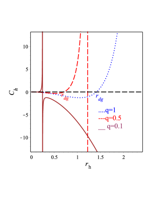
Figure 5: The heat capacity (47) as a function of the horizon $r_{h}$, for solution (III.1) with $c=1$, for various charge choices.

Finally, let us make some comments on the Gibb’s free energy, namely the free energy in the grand canonical ensemble, defined as Zheng and Yang (2018); Kim and Kim (2012)

$$G(r_{h})=E(r_{h})-T(r_{h})S(r_{h}).$$ (49)

Inserting (41), (42) and (43) into (49) we find

$${G_{h}}=\frac{(6q^{2}+cr_{h}^{2})\sqrt{2-c}+\alpha r_{h}(r_{h}^{2}-2q^{2})}{8r_{h}\sqrt{2-c}}.$$ (50)

The behavior of the Gibb’s energy of the black holes (III.1) is presented in Fig. 6 for particular values of the model parameters. As we can see it is always positive when $\alpha>0$ which implies that it is more globally stable.

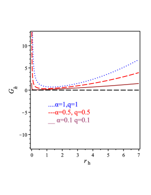
Figure 6: The black hole Gibb’s free energy (50) as a function of the horizon $r_{h}$, for solution (III.1) with $c=1$, for various choices of charge and gravitational modification.

V Discussion and conclusion

The radical advance in multi-messenger astronomy opens the possibility to test general relativity and investigate modified gravity by the gravitational and electromagnetic waves profile that arise form mergers of spherically symmetric objects, such as black holes and neutron stars. Hence, it is crucial to study such object’s properties in various theories of modified gravity in the presence of the Maxwell sector.

In this work we investigated static and rotating charged spherically symmetric solution in the framework of $f({\cal R})$ gravity, allowing additionally the electromagnetic sector to depart from linearity. Applying a convenient, dual description for the electromagnetic Lagrangian, and using as an example the square-root $f({\cal R})$ correction, we were able to solve analytically the involved field equations. The obtained solutions belong to two branches. One that contains the Kerr-Newman metric, namely the rotating charged black hole solution of general relativity, as a particular limit and one that arises purely from the gravitational modification and does not recover the general relativity solution. Moreover, we have shown that the two components of the magnetic fields, of the non-linear electrodynamics, are connected by a constant which if it is vanished we acquire a charged black hole with electric field only Nashed and Capozziello (2019).

Analyzing the novel black hole solution that does not have a general relativity limit we found that it has a true central singularity which is hidden behind a horizon, however for particular parameter regions the horizon disappears and the singularity becomes a naked one, i.e. we obtain a violation of the cosmic censorship theorem.

Furthermore, we investigated the thermodynamical properties of the solutions, such as the temperature, energy, entropy, heat capacity and Gibbs free energy. We extracted the conditions on the gravitational modification parameter in order to obtain entropy and quasilocal energy positivity. Concerning temperature, we showed that it can become negative for particular parameter values, and thus ultracold black holes may be formed. Finally, we examined the thermodynamic stability of the solutions by examining the sign of the heat capacity, extracting the corresponding conditions.

In summary, we showed that even small deviations from general relativity and/or from linear electrodynamics may lead to novel spherically symmetric solution branches, with novel properties that do not appear in standard general relativity. Since these properties may be embedded in the gravitational waves profiles, they could serve as a smoking gun of this subclass of gravitational modification.

References

- Abbott et al. (2016) B. P. Abbott et al. (LIGO Scientific, Virgo), Phys. Rev. Lett. 116, 061102 (2016), eprint 1602.03837.
- Abbott et al. (2017a) B. P. Abbott et al. (LIGO Scientific, Virgo), Phys. Rev. Lett. 119, 141101 (2017a), eprint 1709.09660.
- Abbott et al. (2017b) B. Abbott et al. (LIGO Scientific, Virgo), Phys. Rev. Lett. 119, 161101 (2017b), eprint 1710.05832.
- De Felice and Tsujikawa (2010) A. De Felice and S. Tsujikawa, Living Rev. Rel. 13, 3 (2010), eprint 1002.4928.
- Nojiri and Odintsov (2011) S. Nojiri and S. D. Odintsov, Phys. Rept. 505, 59 (2011), eprint 1011.0544.
- Wheeler (1986) J. T. Wheeler, Nucl. Phys. B 268, 737 (1986).
- Antoniadis et al. (1994) I. Antoniadis, J. Rizos, and K. Tamvakis, Nucl. Phys. B 415, 497 (1994), eprint hep-th/9305025.
- Nojiri and Odintsov (2005) S. Nojiri and S. D. Odintsov, Phys. Lett. B 631, 1 (2005), eprint hep-th/0508049.
- De Felice and Tsujikawa (2009) A. De Felice and S. Tsujikawa, Phys. Lett. B 675, 1 (2009), eprint 0810.5712.
- Lovelock (1971) D. Lovelock, J. Math. Phys. 12, 498 (1971).
- Deruelle and Farina-Busto (1990) N. Deruelle and L. Farina-Busto, Phys. Rev. D 41, 3696 (1990).
- Mannheim and Kazanas (1989) P. D. Mannheim and D. Kazanas, Astrophys. J. 342, 635 (1989).
- Horava (2009) P. Horava, Phys. Rev. D 79, 084008 (2009), eprint 0901.3775.
- Cai et al. (2016) Y.-F. Cai, S. Capozziello, M. De Laurentis, and E. N. Saridakis, Rept. Prog. Phys. 79, 106901 (2016), eprint 1511.07586.
- Bengochea and Ferraro (2009) G. R. Bengochea and R. Ferraro, Phys. Rev. D79, 124019 (2009), eprint 0812.1205.
- Linder (2010) E. V. Linder, Phys. Rev. D81, 127301 (2010), [Erratum: Phys. Rev.D82,109902(2010)], eprint 1005.3039.
- Kofinas and Saridakis (2014) G. Kofinas and E. N. Saridakis, Phys. Rev. D 90, 084044 (2014), eprint 1404.2249.
- Aharony et al. (2000) O. Aharony, S. S. Gubser, J. M. Maldacena, H. Ooguri, and Y. Oz, Phys. Rept. 323, 183 (2000), eprint hep-th/9905111.
- Awad (2006) A. M. Awad, Class. Quant. Grav. 23, 2849 (2006), eprint hep-th/0508235.
- Awad and Johnson (2000a) A. M. Awad and C. V. Johnson, Phys. Rev. D61, 084025 (2000a), eprint hep-th/9910040.
- Awad and Johnson (2000b) A. M. Awad and C. V. Johnson, Phys. Rev. D62, 125010 (2000b), eprint hep-th/0006037.
- Cai et al. (2013) Y.-F. Cai, D. A. Easson, C. Gao, and E. N. Saridakis, Phys. Rev. D 87, 064001 (2013), eprint 1211.0563.
- Anabalon et al. (2014) A. Anabalon, A. Cisterna, and J. Oliva, Phys. Rev. D89, 084050 (2014), eprint 1312.3597.
- Cisterna and Erices (2014) A. Cisterna and C. Erices, Phys. Rev. D89, 084038 (2014), eprint 1401.4479.
- Babichev et al. (2015) E. Babichev, C. Charmousis, and M. Hassaine, JCAP 1505, 031 (2015), eprint 1503.02545.
- El Hanafy and Nashed (2016) W. El Hanafy and G. Nashed, Astrophys. Space Sci. 361, 68 (2016), eprint 1507.07377.
- Brihaye et al. (2016) Y. Brihaye, A. Cisterna, and C. Erices, Phys. Rev. D93, 124057 (2016), eprint 1604.02121.
- Cisterna et al. (2016) A. Cisterna, M. Hassaine, J. Oliva, and M. Rinaldi, Phys. Rev. D94, 104039 (2016), eprint 1609.03430.
- Babichev et al. (2017) E. Babichev, C. Charmousis, and M. Hassaine, JHEP 05, 114 (2017), eprint 1703.07676.
- Cvetković and Simić (2018) B. Cvetković and D. Simić, Class. Quant. Grav. 35, 055005 (2018), eprint 1707.01258.
- Erices and Martinez (2018) C. Erices and C. Martinez, Phys. Rev. D97, 024034 (2018), eprint 1707.03483.
- Cisterna et al. (2017) A. Cisterna, M. Hassaine, J. Oliva, and M. Rinaldi, Phys. Rev. D96, 124033 (2017), eprint 1708.07194.
- Cisterna et al. (2018) A. Cisterna, S. Fuenzalida, M. Lagos, and J. Oliva, Eur. Phys. J. C78, 982 (2018), eprint 1810.02798.
- Gonzalez et al. (2012) P. A. Gonzalez, E. N. Saridakis, and Y. Vasquez, JHEP 07, 053 (2012), eprint 1110.4024.
- Capozziello et al. (2013) S. Capozziello, P. A. Gonzalez, E. N. Saridakis, and Y. Vasquez, JHEP 02, 039 (2013), eprint 1210.1098.
- Iorio and Saridakis (2012) L. Iorio and E. N. Saridakis, Mon. Not. Roy. Astron. Soc. 427, 1555 (2012), eprint 1203.5781.
- Nashed (2013a) G. G. L. Nashed, Phys. Rev. D88, 104034 (2013a), eprint 1311.3131.
- Aftergood and DeBenedictis (2014) J. Aftergood and A. DeBenedictis, Phys. Rev. D90, 124006 (2014), eprint 1409.4084.
- Paliathanasis et al. (2014) A. Paliathanasis, S. Basilakos, E. N. Saridakis, S. Capozziello, K. Atazadeh, F. Darabi, and M. Tsamparlis, Phys. Rev. p. 104042 (2014), eprint 1402.5935.
- Nashed (2015a) G. G. L. Nashed, International Journal of Modern Physics D 24, 1550007 (2015a).
- Nashed (2015b) G. G. L. Nashed, European Physical Journal Plus 130, 124 (2015b).
- Junior et al. (2015) E. L. B. Junior, M. E. Rodrigues, and M. J. S. Houndjo, JCAP 1510, 060 (2015), eprint 1503.07857.
- Kofinas et al. (2015) G. Kofinas, E. Papantonopoulos, and E. N. Saridakis, Phys. Rev. D 91, 104034 (2015), eprint 1501.00365.
- Nashed and El Hanafy (2017) G. G. L. Nashed and W. El Hanafy, Eur. Phys. J. p. 90 (2017), eprint 1612.05106.
- Cruz et al. (2017) M. Cruz, A. Ganguly, R. Gannouji, G. Leon, and E. N. Saridakis, Class. Quant. Grav. 34, 125014 (2017), eprint 1702.01754.
- Awad and Nashed (2017) A. Awad and G. Nashed, JCAP 02, 046 (2017), eprint 1701.06899.
- Ahmed et al. (2016) A. K. Ahmed, M. Azreg-Aïnou, S. Bahamonde, S. Capozziello, and M. Jamil, Eur. Phys. J. C76, 269 (2016), eprint 1602.03523.
- Farrugia et al. (2016) G. Farrugia, J. L. Said, and M. L. Ruggiero, Phys. Rev. D93, 104034 (2016), eprint 1605.07614.
- Koutsoumbas et al. (2018) G. Koutsoumbas, I. Mitsoulas, and E. Papantonopoulos, Class. Quant. Grav. 35, 235016 (2018), eprint 1803.05489.
- Mai and Lu (2017) Z.-F. Mai and H. Lu, Phys. Rev. D95, 124024 (2017), eprint 1704.05919.
- Doneva et al. (2018) D. D. Doneva, S. Kiorpelidi, P. G. Nedkova, E. Papantonopoulos, and S. S. Yazadjiev, Phys. Rev. D 98, 104056 (2018), eprint 1809.00844.
- Awad et al. (2017) A. M. Awad, S. Capozziello, and G. G. L. Nashed, JHEP 07, 136 (2017), eprint 1706.01773.
- Bejarano et al. (2017) C. Bejarano, R. Ferraro, and M. J. Guzmán, Eur. Phys. J. C77, 825 (2017), eprint 1707.06637.
- Abdalla et al. (2019) E. Abdalla, B. Cuadros-Melgar, R. Fontana, J. de Oliveira, E. Papantonopoulos, and A. Pavan, Phys. Rev. D 99, 104065 (2019), eprint 1903.10850.
- Nashed and Saridakis (2019) G. Nashed and E. N. Saridakis, Class. Quant. Grav. 36, 135005 (2019), eprint 1811.03658.
- Destounis et al. (2019) K. Destounis, R. D. Fontana, F. C. Mena, and E. Papantonopoulos, JHEP 10, 280 (2019), eprint 1908.09842.
- Papantonopoulos and Vlachos (2020) E. Papantonopoulos and C. Vlachos, Phys. Rev. D 101, 064025 (2020), eprint 1912.04005.
- Plebański (1970) J. Plebański, Lectures on non-linear electrodynamics: an extended version of lectures given at the Niels Bohr Institute and NORDITA, Copenhagen, in October 1968 (NORDITA, 1970), URL https://books.google.com.eg/books?id=zEZUAAAAYAAJ.
- Ayon-Beato (1999) E. Ayon-Beato, Physics Letters B 464, 25 (1999), eprint hep-th/9911174.
- Salazar I. et al. (1987) H. Salazar I., A. García D., and J. Plebański, Journal of Mathematical Physics 28, 2171 (1987).
- Carroll et al. (2004) S. M. Carroll, V. Duvvuri, M. Trodden, and M. S. Turner, Phys. Rev. D70, 043528 (2004), eprint astro-ph/0306438.
- Cognola et al. (2005) G. Cognola, E. Elizalde, S. Nojiri, S. D. Odintsov, and S. Zerbini, JCAP 0502, 010 (2005), eprint hep-th/0501096.
- Koivisto and Kurki-Suonio (2006) T. Koivisto and H. Kurki-Suonio, Class. Quant. Grav. 23, 2355 (2006), eprint astro-ph/0509422.
- Elizalde et al. (2020) E. Elizalde, G. Nashed, S. Nojiri, and S. Odintsov, Eur. Phys. J. C 80, 109 (2020), eprint 2001.11357.
- Dimitrijevic et al. (2019) I. Dimitrijevic, B. Dragovich, A. Koshelev, Z. Rakic, and J. Stankovic, Phys. Lett. B 797, 134848 (2019), eprint 1906.07560.
- Nashed and Capozziello (2019) G. G. Nashed and S. Capozziello, Phys. Rev. D 99, 104018 (2019), eprint 1902.06783.
- Sebastiani and Zerbini (2011) L. Sebastiani and S. Zerbini, Eur. Phys. J. C71, 1591 (2011), eprint 1012.5230.
- Gamal (2012) G. L. N. Gamal, Chinese Physics Letters 29, 050402 (2012), eprint 1111.0003.
- Nashed (2014) G. G. L. Nashed, EPL 105, 10001 (2014), eprint 1501.00974.
- Nashed (2013b) G. G. L. Nashed, Gen. Rel. Grav. 45, 1887 (2013b), eprint 1502.05219.
- Lemos (1995) J. P. S. Lemos, Phys. Lett. B353, 46 (1995), eprint gr-qc/9404041.
- Awad (2003) A. M. Awad, Class. Quant. Grav. 20, 2827 (2003), eprint hep-th/0209238.
- Nashed et al. (2020) G. Nashed, W. El Hanafy, S. Odintsov, and V. Oikonomou, Int. J. Mod. Phys. D 29, 1750154 (2020), eprint 1912.03897.
- Sheykhi (2012) A. Sheykhi, Phys. Rev. D86, 024013 (2012), eprint 1209.2960.
- Sheykhi (2010) A. Sheykhi, Eur. Phys. J. C69, 265 (2010), eprint 1012.0383.
- Hendi et al. (2010) S. H. Hendi, A. Sheykhi, and M. H. Dehghani, Eur. Phys. J. C70, 703 (2010), eprint 1002.0202.
- Sheykhi et al. (2010) A. Sheykhi, M. H. Dehghani, and S. H. Hendi, Phys. Rev. D81, 084040 (2010), eprint 0912.4199.
- Cognola et al. (2011) G. Cognola, O. Gorbunova, L. Sebastiani, and S. Zerbini, Phys. Rev. D84, 023515 (2011), eprint 1104.2814.
- Zheng and Yang (2018) Y. Zheng and R.-J. Yang, Eur. Phys. J. C78, 682 (2018), eprint 1806.09858.
- Davies (1977) P. C. W. Davies, Proc. Roy. Soc. Lond. pp. 499–521 (1977).
- Babichev et al. (2013) E. O. Babichev, V. I. Dokuchaev, and Y. N. Eroshenko, Phys. Usp. 56, 1155 (2013), [Usp. Fiz. Nauk189,no.12,1257(2013)], eprint 1406.0841.
- Cvetic et al. (2002) M. Cvetic, S. Nojiri, and S. D. Odintsov, Nucl. Phys. B628, 295 (2002), eprint hep-th/0112045.
- Nojiri et al. (2001) S. Nojiri, S. D. Odintsov, and S. Ogushi, Int. J. Mod. Phys. A16, 5085 (2001), eprint hep-th/0105117.
- Nojiri and Odintsov (2002) S. Nojiri and S. D. Odintsov, Phys. Rev. D66, 044012 (2002), eprint hep-th/0204112.
- Nojiri and Odintsov (2017) S. Nojiri and S. D. Odintsov, Phys. Rev. D96 (2017).
- Clunan et al. (2004) T. Clunan, S. F. Ross, and D. J. Smith, Class. Quant. Grav. 21, 3447 (2004), eprint gr-qc/0402044.
- Nojiri et al. (2002) S. Nojiri, S. D. Odintsov, and S. Ogushi, Phys. Rev. D65, 023521 (2002), eprint hep-th/0108172.
- Nouicer (2007) K. Nouicer, Class. Quant. Grav. 24, 5917 (2007), [Erratum: Class. Quant. Grav.24,6435(2007)], eprint 0706.2749.
- Dymnikova and Korpusik (2011) I. Dymnikova and M. Korpusik, Entropy 13, 1967 (2011), ISSN 1099-4300, URL http://www.mdpi.com/1099-4300/13/12/1967.
- Chamblin et al. (1999) A. Chamblin, R. Emparan, C. V. Johnson, and R. C. Myers, Phys. Rev. D60, 064018 (1999), eprint hep-th/9902170.
- Myung et al. (2007) Y. S. Myung, Y.-W. Kim, and Y.-J. Park, Phys. Lett. pp. 221–225 (2007), eprint gr-qc/0702145.
- Dymnikova and Korpusik (2010) I. Dymnikova and M. Korpusik, Phys. Lett. pp. 12–18 (2010).
- Berej et al. (2006) W. Berej, J. Matyjasek, D. Tryniecki, and M. Woronowicz, Gen. Rel. Grav. 38, 885 (2006), eprint hep-th/0606185.
- Man and Cheng (2014) J. Man and H. Cheng, Gen. Rel. Grav. 46, 1660 (2014), eprint 1304.5686.
- Tharanath et al. (2015) R. Tharanath, J. Suresh, and V. C. Kuriakose, Gen. Rel. Grav. 47, 46 (2015), eprint 1406.3916.
- Maluf and Neves (2018) R. V. Maluf and J. C. S. Neves, Phys. Rev. p. 104015 (2018), eprint 1801.02661.
- Kim and Kim (2012) W. Kim and Y. Kim, Phys. Lett. B718, 687 (2012), eprint 1207.5318.