Distributed ADMM with linear updates over directed networks*
Abstract
We propose a distributed version of the Alternating Direction Method of Multipliers (ADMM) with linear updates for directed networks. We show that if the objective function of the minimization problem is smooth and strongly convex, our distributed ADMM algorithm achieves a geometric rate of convergence to the optimal point. Our algorithm exploits the robustness inherent to ADMM by not enforcing accurate consensus, thereby significantly improving the convergence rate. We illustrate this by numerical examples, where we compare the performance of our algorithm with that of state-of-the-art ADMM methods over directed graphs.
I Introduction
In this paper, we focus on solving an unconstrained optimization problem of the form
| (P1) |
where is the decision variable. The computations involved in solving the problem are performed by a group of agents which form a communication network. Due to the restrictions imposed by the network, an agent can communicate only with its neighbours in the network. For each , is a convex function privately known to agent . The goal of each agent is to solve (P1) in cooperation with its neighbours, without explicitly revealing its function . This restriction on the exchange of ’s could arise due to privacy reasons or due to the communication cost involved in such an exchange. Since each agent minimizes the sum of all functions, it computes a “globally optimal” solution without revealing its own function to other agents. Such distributed optimization problems are encountered in several applications such as achieving average consensus in a distributed manner, distributed power system control, formation control of robots, statistical learning etc [12].
Distributed optimization problems have been widely studied in the literature. Existing methods for solving these problems can be broadly classified into two types: gradient-descent-based primal methods [11, 13, 6] and Lagrangian-based dual-ascent methods [14, 7, 8, 4]. While most of the methods in the literature assume that the communication network is undirected [14, 7, 8], i.e., communication links between agents are bidirectional; in practice, the network is often directed, i.e., the links are unidirectional. This can occur, for example, if two agents have different broadcast ranges. Generalizing distributed optimization algorithms, which work for undirected graphs, to directed graphs is not straightforward, and in the past has required the introduction of some novel concepts. For example, gradient-descent methods were generalized to directed networks by introducing new concepts such as balancing weights [6], push-sum [11], push-DIGing (Distributed In-exact Gradient tracking) [13] etc. On the other hand, there has been less progress in generalizing Lagrangian-based methods to directed graphs.
A special type of Lagrangian-based dual-ascent method is the Alternating Direction Method of Multipliers (ADMM). Compared to the standard dual-ascent method, ADMM is more robust and amenable to parallel implementation in a multi-agent setting [1]. While, distributed implementation of ADMM is well-studied for undirected graphs [14, 7], an extension to directed graphs was non-existent in the literature (see [13]), until recently. In the past few years, to the best of our knowledge, two methods for distributed ADMM over directed graphs have been proposed: DC-DistADMM (Directed Constrained Distributed ADMM) in [4], and D-ADMM-FTERC (Distributed Alternating Direction Method of Multipliers using Finite-Time Exact Ratio Consensus) in [2].
The key differences between our method, and DC-DistADMM [4] and D-ADMM-FTERC [2] are as follows.
-
•
At each iteration of the respective algorithms, DC-DistADMM requires that, for a fixed , the agents reach consensus up to an -accuracy, while D-ADMM-FTERC requires that the agents reach exact consensus. As noted earlier, ADMM is known to be robust to errors in implementation [1]. For this reason, we do not enforce any accuracy on the consensus step. Instead, we require the agents to communicate with each other times per iteration. The value of is chosen depending on other parameters of the algorithm. However, it is observed in simulations that even with , the algorithm performs well in the sense that it gives a convergence rate that is better than that of DC-DistADMM and D-ADMM-FTERC.
-
•
Instead of the push-sum and finite-time ratio-consensus methods, we use the method of balancing weights to achieve consensus among the agents. The balancing weights are updated dynamically in a distributed manner. While the operations involved in push-sum and ratio-consensus methods involve divisions, which may cause numerical issues, the balancing weights method involves only addition and multiplication (linear updates), and hence does not suffer from these problems.
- •
Our main contributions to the literature are as follows.
-
•
We propose an ADMM algorithm (Algorithm 1) which solves the optimization problem (P1) in a distributed manner over directed networks. At each iteration, our algorithm runs an “inner loop” where each agent computes an approximate average of the primal variable iterates of all agents in a distributed manner. This approximate consensus step exploits the inherent robustness of ADMM, resulting in a superior performance compared to other distributed ADMM algorithms in [4], [2].
- •
- •
The rest of the paper is organized as follows. In Section II, we propose a problem equivalent to (P1) that is amenable to distributed implementation. In Section III, we present our distributed ADMM algorithm for solving this equivalent problem. In Section IV, we state our main result which guarantees convergence of the algorithm. We also give an outline of the proof of this result. In Section V, we present some numerical examples to compare the performance of our algorithm with some other ADMM algorithms over directed graphs. Finally, we give some concluding remarks in Section VI. Proofs of all the results can be found in the appendix.
Notation: Let denote logarithm with base . be the vector of all ones in . For a vector , be the th element of , be the transpose of and let denote the -norm of .
For a matrix , let denote its th row. Let be its Frobenius norm and be its induced -norm. Given two matrices and , let be their Frobenius inner-product. Given a vector , let be the diagonal matrix with elements on the diagonal.
For a function , let denote the convex conjugate of defined as for all such that the supremum is finite. Let be the gradient of at defined as .
We use the shorthand to denote the sequence .
II Problem Formulation
Consider a set of agents denoted by . The communication pattern between the agents is depicted by a directed graph , where is the set of all directed edges. We denote if there exists a directed edge from agent to agent . Following assumption is standard in the literature when agents desire to reach consensus over a directed graph, e.g., [6, 8, 11].
Assumption 1.
is strongly connected, i.e., there exists a directed path between each pair of agents.
The agents must cooperatively solve the optimization problem (P1), which can be equivalently written as
| (P2) | ||||||
where is the convex function known only to agent , and is the decision variable of agent . The constraint is called the consensus constraint. To write (P2) in a compact form, let be the matrix of all decision variables. Then, the consensus constraint can be written as
Further, let . Then, (P2) can be written as
| (P3) | ||||||
We assume that (P3) is solvable, i.e., there exists an optimal point of (P3). We make the following assumptions on the function . These assumptions are standard in the literature whenever a geometric rate of convergence is desired, e.g., [13, 8, 7].
Assumption 2.
For each the function is -strongly convex, i.e., such that for all ,
Further, for each , is differentiable and is -Lipschitz, i.e., such that for all ,
An immediate consequence of Assumption 2 is that is -strongly convex and is -Lipschitz.
The next two steps ensure that our ADMM algorithm to solve (P3) can be executed in a distributed and parallel manner over the directed graph . First, we introduce a new variable and write (P3) as
| (P4) | ||||||
This decouples the decision variables of the agents from each other. Second, we move the constraint into the objective function using an indicator function as follows. Define
Now, (P4) is equivalent to
| (P5) | ||||||
The formulation above enables us to impose the constraint explicitly at each step of the ADMM algorithm, as we shall see later. Since is strongly convex under Assumption 2, (P5) has a unique optimal point which satisfies .
To solve (P5) using ADMM, we define the augmented Lagrangian of the problem as
| (1) |
where is the dual variable associated with the constraint and is the penalty parameter. The term is called the penalty term. Let be a dual optimal point of (P5). In the next section, we propose our distributed ADMM algorithm which generates sequences and of primal-dual iterates which converge to and respectively, at a geometric rate.
III Algorithm
We begin by writing the standard 2-block ADMM algorithm (see [1]) for (P5) as follows. For simplicity, all iterates are initialized at zero. For each ,
| (2) | ||||
| (3) | ||||
| (4) |
We assume that for all , each agent maintains the set of iterates . To implement the algorithm above in a distributed manner, each agent must update its iterates using only the information received from its in-neighbours. We analyze each update step above to see if such a distributed implementation is possible.
The update step: Substituting for from (1) in
(2), we obtain
| (5) |
Note that, by definition, can be decomposed as . Hence, the update step above is equivalent to
| (6) |
for all , which can be implemented parallely.
The update step: We can derive an explicit expression for in (3) as shown by the following result.
Lemma 1.
The update step given in (3) is equivalent to
| (7) |
The proof of Lemma 1 can be found in Appendix VII. Note that (7) involves computing an average for each iteration. We use the idea of balancing weights [6], along with a dynamic average consensus type update rule [16] to compute an estimate of in a distributed manner. This has been proposed earlier for primal gradient tracking, e.g., [6, 13]. We use these techniques to track the average of the dual variable.
Our update rule to estimate is as follows. Consider an agent and an iteration . Let the agent’s estimate of be denoted by . This estimate is updated dynamically. Let the estimate be initialized as .111We use the notation . The intuition behind this initialization is to perturb , the last-known estimate of the average, by , the change in agent ’s contribution to the average. Such an initialization is typical of a dynamic average consensus type update rule [5]. Note that this initialization implicitly assumes that agent knows the exact value of , which may not be possible. This assumption can be relaxed with the following observation. From (4), we know that . Hence, . Thus, initializing the estimate only requires the knowledge of , which the agent has from the update performed in (6). Now, agent updates its estimate as follows. Consider an integer , which must satisfy a lower-bound to be specified later. In each iteration , the agents run an “inner loop” number of times where they communicate and update their estimate . Specifically, for all and ,
| (8) |
where is the out-degree of agent , and is the weight used by agent to scale its outgoing information. Thus, agent ’s estimate is computed iteratively by taking a weighted average of its own estimate with those of its in-neighbours. To ensure that the agents reach consensus when the underlying graph is directed, the weights must be chosen appropriately. One such set of weights are the “balancing weights” of a graph. We next describe our update rule used to compute the weights in (III), as introduced in [6].
Let be the diagonal matrix of out-degrees of the agents. Let be the adjacency matrix of the graph, i.e., if and otherwise. Given a vector of weights, let be the weight matrix associated with .
Definition 1.
(Balancing weights) Given a graph , a vector is said to be a vector of balancing weights for if the weight matrix associated with is doubly-stochastic, i.e., .
We use the same update rule as described in [6] to compute the set of weights required in (III). Let be the maximum out-degree of the graph and be the diameter of the graph. Following [6], we initialize the weights as . Then, for all and ,
| (9) |
and . Thus, agent ’s weight is updated by taking a weighted average of its own weight with those of its in-neighbours. Hence, (9) can be implemented in a distributed manner. Note that for each iterate , the update rule above is implemented sequentially after implementing (III).
The update rule in (9) can be written compactly as
| (10) |
and , where . Further, the update rule in (III) can be written compactly as
| (11) |
where and is the weight matrix associated with the weights . It is known that the weights updated according to (10) converge to the set of balancing weights of the graph [6]. Additionally, we require that the weight matrix satisfies certain properties. These properties are stated in our next result.
Lemma 2.
Let be the weight matrix associated with the weights updated as per (10). The matrix has the following properties.
-
1.
For all , for all , such that , and .
-
2.
such that for all , for all .
-
3.
For all , .
-
4.
such that for all , for all .
The proof of Lemma 2 can be found in Appendix VIII. In essence, Lemma 2 states that is left-stochastic, while its right eigenvector associated with the eigenvalue converges to as . Further, for large , has a bounded norm and its second-largest eigenvalue is strictly inside the unit circle.
Finally, we look at the distributed implementation of the dual update step.
The update step: From (4), we have . Thus, each agent can compute independently using its set of iterates .
Remark 1.
The agents need to communicate with their neighbours only during the update step.
The steps implemented by each agent are summarized in Algorithm 1.
IV Main Result
In this section, we state our main result and then give an outline of its proof. The details of the proof can be found in the appendix.
Theorem 1.
Given a problem of the form (P5), suppose that the parameters of Algorithm 1 are chosen such that the number of communication rounds per iteration, , satisfies
| (12) |
the convergence rate satisfies
| (13) |
and the penalty parameter satisfies
| (14) |
where
is arbitrary, , are as defined in Lemma 2, and and are as defined in Assumption 2. Then, the iterates generated by Algorithm 1 satisfy
for some non-negative constants , where is the unique primal-dual optimal point of (P5).
Remark 3.
Remark 4.
If is -strongly convex and -smooth (as is the case due to Assumption 2), then is called the condition number of . We can argue that the convergence of Algorithm 1 is faster if the problem is well-conditioned, i.e., is small. To see this, note that with a decrease in , the LHS of (13) decreases, while the RHS increases (since increases). Thus, smaller values of give a wider range of values of the convergence rate that satisfy (13).
The proof of Theorem 1 uses the small gain theorem. This proof is inspired by the ideas in [13] and [8]. We briefly recall the theorem after introducing some notation. Given a sequence of matrices in and a convergence rate , let
| (15) |
for all . Further, given two sequences and a constant , we use the notation to denote for all , for some constant . Now, the small gain theorem can be stated as follows.
Proposition 1.
[13, Theorem 3.7] (Small gain theorem) Given sequences of vectors in , suppose there exist non-negative constants and a convergence rate satisfying the cycle of relations
such that . Then, there exist constants such that for all .
Note that, if the conditions of the small gain theorem are satisfied, then at a geometric rate of for all . Our main result is stated below.
We use the small gain theorem to prove Theorem 1 as follows. Let
To show that and with a geometric rate of , it is enough to show that and are bounded. To show this, we first prove that there exist non-negative numbers such that the cycle of relations
| (16) |
holds with , where for all . The proof of each arrow in (16) is provided in Appendix X. In particular, we show that the conditions given in Theorem 1 are sufficient to prove the cycle of relations in (16) such that . Then, by the small gain theorem (Proposition 1), it follows that and are bounded.
V Numerical Examples
The observations noted in this section were made across many examples. For simplicity, we present the results from one such example.222The datasets generated during the current study are available from the corresponding author on request.
V-A Sensor network
Problem setup: We consider a sensor network of agents. Each agent is placed in the unit square uniformly at random, and it is assigned a random broadcast range between and . This generates a directed graph. We consider the problem of sensor fusion, where the goal of all the agents is to estimate a common parameter using data from the neighbouring agents. The local objective function of agent is , where the measurement matrix and the data matrix are generated randomly from a standard normal distribution. To estimate the parameter, the agents must solve problem (P1) in a distributed manner.
Algorithms chosen for comparison: We consider DC-DistADMM [4] and D-ADMM-FTERC [2]. Note that the bounds on the parameters of each of these algorithms, such as the ones on and given in Theorem 1, are often very conservative. Hence, we tune the parameters to get the best convergence rate, as suggested in [13] .
Convergence rate: A plot of the normalized primal residual obtained by each of the algorithms mentioned above is shown in Fig. 1 (left). It can be observed that the performance of Algorithm 1 is better than that of D-ADMM-FTERC and DC-DistADMM in this example.
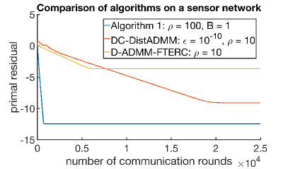
It is worth noting that the algorithms mentioned above also generate a sequence of dual variable iterates which converge to the dual optimal point (not shown here due to space constraints). This is not the case with gradient-based algorithms.
Communication cost: For each algorithm, the number of values sent by an agent per communication round is , where is the dimension of the unknown parameter.
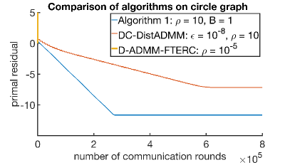
V-B Graphs with large diameters
Most of the graphs observed in practice are sparse and hence have large diameters. It was observed that Algorithm 1 performs much better than DC-DistADMM and D-ADMM-FTERC on graphs with large diameters, such as a directed circle graph and an undirected line graph. The residuals generated by each algorithm on a directed circle graph of agents are shown in Fig. 1 (right). Note that the residual generated by D-ADMM-FTERC did not converge to zero despite tuning the value of the step size to . The intuition behind the superior performance of Algorithm 1 is as follows. It is known that the error in consensus after steps is upper-bounded by , where is the second-smallest eigenvalue of the weight matrix used to achieve consensus [15]. Further, has a lower-bound that is inversely proportional to the diameter of the graph [10]. Thus, graphs with larger diameters take more iterations to achieve consensus. Algorithm 1 does not require any accuracy on the inner consensus loop, while the other algorithms require either exact consensus or -consensus at each step. ADMM appears to be robust to errors in consensus. Hence, enforcing consensus accuracy at each iteration may be an overkill.
V-C Sensitivity of Algorithm 1 to its parameters
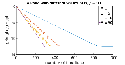
Effect of : We study the effect of changing the number of communication rounds per iteration () in the inner loop of our ADMM algorithm. As observed in Fig. 2 (left), with an increase in , the number of iterations required to reach the optimal value decreases, while there is no change in the final value.
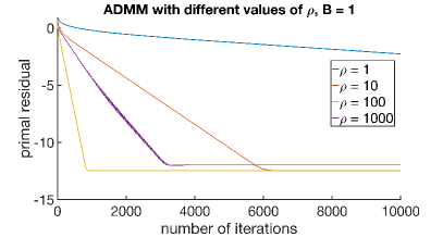
Robustness to changes in : We observe in Fig. 2 (right), that the primal residual decreases monotonically for a large range of values of , albeit with different rates. On the other hand, primal-descent algorithms are known to be sensitive to their step-size.
VI Conclusion
We proposed an ADMM algorithm to solve distributed optimization problems over directed graphs. Our algorithm uses the ideas of balancing weights and dynamic average consensus. Under the assumption that the objective function is strongly convex and smooth, we showed that the primal-dual iterates of the algorithm converge to their unique optimal points at a geometric rate, provided the parameters of the algorithm are chosen appropriately. Through a numerical example, we demonstrated that our algorithm gives a better performance than some state-of-the-art ADMM methods over directed graphs. Additionally, the algorithm was observed to be robust to changes in its parameters. In the future, it will be interesting to see if convergence of the algorithm can be guaranteed by relaxing the assumptions of strong convexity and smoothness. Further, it will be interesting to extend the algorithm to time-varying graphs.
References
- [1] Stephen Boyd, Neal Parikh, Eric Chu, Borja Peleato, and Jonathan Eckstein. Distributed optimization and statistical learning via the alternating direction method of multipliers. Found. Trends Mach. Learn., 3(1):1–122, January 2011.
- [2] Wei Jiang and Themistoklis Charalambous. Fully distributed alternating direction method of multipliers in digraphs via finite-time termination mechanisms. arXiv preprint arXiv:2107.02019, 2021.
- [3] Sham Kakade, Shai Shalev-Shwartz, and Ambuj Tewari. On the duality of strong convexity and strong smoothness: Learning applications and matrix regularization. Unpublished Manuscript, 2009.
- [4] Vivek Khatana and Murti V. Salapaka. DC-DistADMM: ADMM algorithm for constrained optimization over directed graphs. IEEE Transactions on Automatic Control, pages 1–16, 2022.
- [5] S. S. Kia, B. Van Scoy, J. Cortes, R. A. Freeman, K. M. Lynch, and S. Martinez. Tutorial on dynamic average consensus: The problem, its applications, and the algorithms. IEEE Control Systems Magazine, 39(3):40–72, 2019.
- [6] A. Makhdoumi and A. Ozdaglar. Graph balancing for distributed subgradient methods over directed graphs. In 2015 54th IEEE Conference on Decision and Control (CDC), pages 1364–1371, 2015.
- [7] A. Makhdoumi and A. Ozdaglar. Convergence rate of distributed ADMM over networks. IEEE Transactions on Automatic Control, 62(10):5082–5095, 2017.
- [8] M. Maros and J. Jaldén. PANDA: A dual linearly converging method for distributed optimization over time-varying undirected graphs. In 2018 IEEE Conference on Decision and Control (CDC), pages 6520–6525, 2018.
- [9] Carl D. Meyer. Matrix Analysis and Applied Linear Algebra. Society for Industrial and Applied Mathematics, USA, 2000.
- [10] Bojan Mohar. Eigenvalues, diameter, and mean distance in graphs. Graphs and combinatorics, 7(1):53–64, 1991.
- [11] A. Nedić and A. Olshevsky. Distributed optimization over time-varying directed graphs. IEEE Transactions on Automatic Control, 60(3):601–615, 2015.
- [12] Angelia Nedić and Ji Liu. Distributed optimization for control. Annual Review of Control, Robotics, and Autonomous Systems, 1(1):77–103, 2018.
- [13] Angelia Nedić, Alex Olshevsky, and Wei Shi. Achieving geometric convergence for distributed optimization over time-varying graphs. SIAM Journal on Optimization, 27(4):2597–2633, 2017.
- [14] E. Wei and A. Ozdaglar. On the convergence of asynchronous distributed alternating direction method of multipliers. In 2013 IEEE Global Conference on Signal and Information Processing, pages 551–554, 2013.
- [15] Lin Xiao and Stephen Boyd. Fast linear iterations for distributed averaging. Systems & Control Letters, 53(1):65 – 78, 2004.
- [16] Minghui Zhu and Sonia Martínez. Discrete-time dynamic average consensus. Automatica, 46(2):322 – 329, 2010.
APPENDIX
VII Proof of Lemma 1
The update step in (3) can be written as
| (18) |
We parameterize the constraint set of (18), i.e., , using the parameter as . With this parameterization, let be the minimizer of (18). We show that as follows. By definition,
This implies
where we have used the fact that the matrices and are orthogonal. Thus, we have , i.e., for all .
VIII Proof of Lemma 2
(1) The statement follows from the fact that, by definition, is column stochastic.
(2) It is shown in [6, Lemma 1] that exists. Hence, exists and is independent of . This implies exists and is independent of . Let . Now, by the triangle inequality,
| (19) |
We analyze each term in the RHS of (VIII) one-by-one.
(a) : By definition of , as .
(b) : It is shown in [6, Lemma 1] that is a doubly-stochastic matrix. Further, it is shown in [6, Lemma 2] that is a non-negative matrix with for all and if and only if . Using these facts, we first show that is a primitive matrix. To show this, it is enough to show that is a positive matrix, where is the diameter of . For any ,
By definition, is the length of the largest path connecting any two nodes. Moreover, is strongly connected. Hence, any given , there exists a path from to . Hence,
Thus, is a positive matrix. Now, . Thus, is also a positive matrix. It then follows that is a primitive matrix. This implies [9, (8.3.16)]. Now,
where we have used the facts as shown in [6, Lemma 1]. Thus, .
(c) : Consider any . We show that such that for all . For all and ,
| (20) |
We argued above that is a primitive matrix with and . Hence, . It follows that such that for all [9, (8.3.10)]. Following the same arguments as with above, we can show that for all and . Hence, for all , such that for all . Moreover, since , the eigenvalues of converge to those of . This implies is independent of (see [9, (8.3.10)], which implies that the rate of convergence of to depends only on the second largest eigenvalue ). Now, let . Note that given any matrix , is a continuous function of the entries of . Hence, implies such that for all . Substituting the aforementioned facts in (VIII), we have for all . This implies as .
Using the results derived for each of the three terms above, from (VIII) we can conclude that for large-enough.
(3) The statement follows from the fact that as , which we have proved above.
(4) For all , . Now, choosing implies for all . On the other hand, is bounded since converges to . Thus, for all for some .
IX Some intermediate results
We state some useful intermediate results.
Lemma 3.
Let , , be sequences in such that for all . Suppose for some constant , for all . Then, for all .
Proof.
Since is a non-negative sequence for all and , we have
for all . Now, using , we obtain
∎
Let denote the conjugate of , i.e., for all such that the supremum is finite.
Lemma 4.
The dual optimal point of (P5) satisfies .
Proof.
Lemma 5.
Proof.
From the definition of , we have
This implies
| (21) |
Now, from the update step (5) of Algorithm 1, we have, for all ,
Using (4), this implies
Hence, we have
Now, using above relation with (IX) gives , which is the first part of the lemma. Next, by definition of a primal-dual optimal point, we have
where is the Lagrangian of (P5) (equation (1) with ). This implies . Using this relation with (IX), it follows that . ∎
X Proof of each arrow in (16)
Proof of the first arrow (): From Proposition 2, we obtain that for all ,
Using Lemma 5 with the relation above, we have
| (22) |
Further, . Substituting this relation in (22), we have
| (23) |
Hence,
| (24) |
for all . Thus, .
Proof of the second arrow (): Using the update rule (11) of and the first property in Lemma 2, we have, for all and ,
Hence,
This implies
where . This implies
Since and , we have . Further, by the second property in Lemma 2, , such that for all , . Hence, for all ,
Now, by the third property in Lemma 2, we know that . Since is a continuous function, there must exist a such that for all , . Using this inequality iteratively from to , we have for all . By definition, and . Hence, the last inequality is equivalent to for all . Hence, for all ,
for some constant . Thus, .
Proof of the third arrow (): We prove the third arrow in two steps. In the first step, we bound by a linear combination of and . In the second step, we bound by a linear combination of and . To complete the proof, we use the two bounds together.
Step 1: Using triangle inequality,
We know that for all . Hence,
From (23), we know that for all . Using this with Lemma 5 and Proposition 2, we have
Hence,
Dividing by on both sides, we have
for all . Taking supremum over , we have
for all for some constant . Rearranging the terms, we have
From (14), we know that . Hence,
| (25) |
Step 2: Let . For all ,
This implies
| (26) |
We try to bound the term above. The update step in Algorithm 1 can be written as
From Lemma 4, we know that . Evaluating the optimality condition for the minimization problem above at , we obtain
Using Lemma 5, this implies
| (27) |
For the ease of notation, let . Now, we bound the term . Since is -strongly convex, we have, for all in the domain of , . This implies
where the last inequality follows by using Peter-Paul inequality on , where is arbitrary. Similarly, using the fact that is -smooth, we have, for all in the domain of ,
where is arbitrary. Adding the two inequalities above with , we have
Substituting this in (X), and then substituting (X) in (26), we obtain
| (28) |
Choose . Further, since is -strongly convex,
where , since and . Thus,
Substituting the inequality above in (X), dividing by on both sides and taking supremum over , we obtain
for all , for some constant . From (14), we know that . Hence, using Lemma 3, we have
| (29) |
for all . Substituting (X) in (X), we obtain that
for all , for some . Rearranging the terms, we obtain that
where
It can be verified that given (14), since
we have . Hence,
| (30) |
for all , for some and
Substituting the inequality above in (X), we obtain
for all , for some . Thus, for all ,
for some and
| (31) |