Dynamical Landscape and Multistability of a Climate Model

Abstract

We apply two independent data analysis methodologies to locate stable climate states in an intermediate complexity climate model and analyze their interplay. First, drawing from the theory of quasipotentials, and viewing the state space as an energy landscape with valleys and mountain ridges, we infer the relative likelihood of the identified multistable climate states, and investigate the most likely transition trajectories as well as the expected transition times between them. Second, harnessing techniques from data science, specifically manifold learning, we characterize the data landscape of the simulation output to find climate states and basin boundaries within a fully agnostic and unsupervised framework. Both approaches show remarkable agreement, and reveal, apart from the well known warm and snowball earth states, a third intermediate stable state in one of the two climate models we consider. The combination of our approaches allows to identify how the negative feedback of ocean heat transport and entropy production via the hydrological cycle drastically change the topography of the dynamical landscape of Earth’s climate.

1 Introduction

The climate, an extremely high-dimensional complex system, is determined by five interacting subdomains: a gaseous atmosphere, a hydrosphere (water in liquid form), a lithosphere (upper solid layer), a cryosphere (water in solid form) and a biosphere (ecosystems and living organisms) (1). The climate is driven by the inhomogeneous absorption of incoming solar radiation and can be treated as a highly non-trivial dynamical system that features spatio-temporal variability on a vast range of scales. The system is at an approximate nonequilibrium steady state due to the resulting interplay of forcings, dissipation, positive and negative feedbacks, instabilities and saturation mechanisms (2). The presence of periodic as well as irregular fluctuations in the boundary conditions does not allow the climate to reach an exact steady state (3; 4).

A straightforward attempt to mathematically formulate the dynamics of the climate system is by defining a set of partial differential equations (PDEs) that describe the budget of mass, momentum and energy. As this set of PDEs is impossible to solve analytically, they are usually simulated numerically. Depending on the number of resolved variables, this procedure is extremely challenging both from a technological and scientific point of view, and requires a diversified approach. Therefore, a hierarchy of climate models can be established (5; 6; 7; 8). At the lowest level of such a hierarchy one can find simple zero or one-dimensional Energy Budget Models (EBMs) that model the energy exchange in the atmosphere or triggered by the solar radiation (9; 10; 11), as well as low-dimensional models that represent fundamental processes of the large scale oceanic (12; 13; 14) and atmospheric dynamics (15; 16; 17). Next come the so-called intermediate complexity models, which provide a parsimonious yet Earth-like representations of the dynamics of climate, see e.g. (18; 19; 20; 21). Finally, modern state-of-the-art climate models, similar to the ones featured in the latest Intergovernmental Panel on Climate Change (IPCC) report (22) are based on applying a series of necessary truncations and approximations in such a set of PDEs. In general, the impact of the neglected scales of motions on the explicitly resolved scales is approximated via suitably developed parametrizations, which include deterministic, stochastic, and possibly non-Markovian components (23).

1.1 Global Stability Properties of the Climate System

The current astronomical configuration of Earth supports the present day Warm (W) climate, and a frozen one, termed Snowball (SB), which exhibits global glaciation, extremely low temperatures and limited climatic variability. Geological and paleomagnetic evidence suggests that during the Neoproterozoic era (in particular around 630 and 715 million years ago), the Earth exhibited at least two major long lasting global glaciation periods, thus entering twice into the snowball climate state (24; 25). Simple energy balance models are able to reproduce the associated multistability of the climate system (9; 10; 11), which is mainly affected by the so-called ice-albedo feedback. The importance of such a mechanism is confirmed by studies of higher complexity models (26; 27; 28; 24; 29).

If we now focus on the current climate or the climate of the recent past (thus within the W state), the Earth is well-known to feature further elements of multistability associated with critical transitions among stable states. Examples of geographically localized phenomena affecting the climate system featuring such a behaviour – the so-called tipping elements (30) – include the dieback of the Amazon forest (31), the shut-down of the thermohaline circulation of the Atlantic ocean (32), the methane release resulting from the melting of the permafrost (33), and the collapse of the atmospheric circulation regime associated to the Indian monsoon (34). A critical transition taking place for one climatic subsystem may trigger the tipping of another element: this is the phenomenon of so-called cascading tipping points (35; 36).

Transitions between metastables states might be facilitated by mechanisms like stochastic resonance (37), which has been recently reframed according to the formalism adopted here for treating nonequilibrium systems (38). Indeed, stochastic resonance is thought to act in the climate system at different spatial and temporal scales, ranging from ultralong (39; 40; 41), to intermediate (42; 43; 44; 45), to short ones (46; 47; 48).

In this work, we explore the multistability of a climate model through methods from nonequilibrium statistical physics, dynamical systems, and data science, pushing forward the scientific programme presented in (4; 49) We then take inspiration from the Waddington’s “epigenetic landscape” metaphor in evolutionary biology (50; 51; 52; 53). The phase space of the climate model can be explored by adding suitably defined stochastic forcing. As a result, the competing metastable climatic states can be viewed as vast valleys of a quasi-potential landscape $\Phi$, separated by mountain ridges, corresponding to unstable climates (54; 49). The stochastic forcing allows for exploring the landscape and, in particular, makes it possible to observe transitions between the metastable states.

Unfortunately, the actual evolution of the climate system cannot be fully regarded as the idealised stochastic motion in a fixed nonequilibrium quasi-potential landscape described above because geological, biological, astronomical, and astrophysical factors modulate the landscape on a vast range of time scales. Nonetheless, the quasi-potential landscape viewpoint can be extremely useful to understand its multistability at an instance in time.

1.2 Outline of the Paper

In this paper we will study the transitions between competing metastable states of PLASIM (55), a simplified climate model that has shown extreme flexibility in describing the dynamics of a vast range of climate conditions, including very exotic ones (56; 57; 58; 59; 60; 61). The model features O($10^{5}$) degrees of freedom (d.o.f.).

We consider two setups of the model – one allowing for the ocean to transport heat from low to high latitudes (setup A), previously used in (60), and one where only the atmosphere is able to perform large scale heat transport (setup B), previously used in (59). The main limitation of the model in both setups is its lack of explicit representation of the deep ocean circulation, which is of great relevance for the dynamics of the present climate on centennial to millennial time scales.

We explore the phase space of the model by allowing the solar irradiance $S^{*}$ to randomly fluctuate around the present-day mean value of $S^{*}=1365\,\textrm{W}/\textrm{m}^{2}$, thus triggering transitions among the competing climate states. Along the lines of (54; 49), we construct the quasipotential of the stochastically perturbed system (62; 63; 64; 65). and we compute the transitions paths among attractors composed of instantonic and relaxation trajectories by averaging over many transition events.

The identification of the competing attractors is approached in two ways. First, we use standard forward numerical modelling and identify different asymptotic states, associated with separate basins of attraction, when stochastic forcing is removed from the system. Second, competing attractors are automatically detected through data-driven methods applied to the output of long stochastic integrations of the model. Such methods have been used for studying metastable states in biomolecules, and allow one to reconstruct very effectively the quasi-potential $\Phi$ of the system, partially taking care of the curse of dimensionality (66; 67; 68; 69). We anticipate that whereas in setup A we find the two usual W and SB states, we discover that setup B features the presence of a third stable climate state (to be termed “cold climate” (C) in the following), with an ice free latitudinal band at roughly $\pm\,20^{\circ}$ around the Equator and mild, larger than $10^{\circ}$C surface temperatures, along with vigorous atmospheric circulation and non-trivial hydrological cycle in the same band. Such a third state resembles previously suggested exotic climatic configurations such as the slushball Earth (26) and the Jormungand state (28). The C state corresponds to a shallow minimum of the quasipotential and disappears when ocean transport is included in the system, which acts as a strong stabilizing mechanism. The presence of the C state has important implications both on the statistical mechanics of the system and on the topology of the transition paths between the W and the SB states.

The paper is structured as follows. Section 2 contains the mathematical framework behind our analysis. Section 3 provides a description of the climate model used in this study. Section 4 contains the description and critical analysis of the obtained results. Section 5 is dedicated to drawing the conclusion of this work and to presenting future research perspectives. The electronic supplementary material (ESM) attached to this paper, accessible here, contains some extra information on the computation of the average transition paths and a brief and informal description of the mathematics of the transfer operator and of its finite-size representation. Additionally, it includes a set of movies related to the numerical simulations performed in this study.

2 Qualitative and Quantitative Aspects of the Multistability of the Climate System

2.1 Dynamical Landscape of the Climate System

A multidimensional deterministic dynamical system can be defined as a set of ordinary differential equations

$$\frac{\mathrm{d}\bm{x}}{\mathrm{d}t}=\bm{F}(\bm{x},t),\qquad\bm{x}(t=0)\equiv\bm{x}_{0},$$ (1)

where $\bm{x}(t)\in\mathbb{R}^{N}$ describes the state of the system at time $t$ with initial condition $\mathbf{x}_{0}$, and $\bm{F}(\bm{x},t)\in\mathbb{R}^{N}$ is a smooth vector field. The initial condition $\bm{x}_{0}$ determines the asymptotic state of its orbit. If Eq. (1) possesses more than one asymptotic states, defined by the attractors $\Omega_{j}$, $j=1,\ldots,J$, the system is multistable. The phase space is partitioned between the basins of attraction $B_{j}$ of the attractors $\Omega_{j}$ and the boundaries $\partial B_{l}$, $l=1,\ldots,L$ separating such basins, which possess a set of saddle points $\Pi_{l}$, $l=1,\ldots,L$. Such saddle points attract initial conditions on the basin boundaries (70; 71; 72) and can be computed using the so-called edge tracking algorithm (73), which was used in an EBM by (74). Chaotic unstable saddles, then termed Melancholia (M) states, have been constructed with the edge tracking algorithm for a simplified climate model built by coupling a primitive equation atmosphere with a diffusive ocean (29).

Escaping an attractor is possible if the system is forced by a properly defined stochastic forcing (75; 76; 77) . By subjecting Eq. (1) to a Gaussian random noise and considering it in Itô form, we write the stochastic differential equation

$${\mathrm{d}{\bm{x}}}=\bm{F}(\bm{x})\mathrm{d}t+\sigma\bm{s}(\bm{x})\mathrm{d}\bm{W},$$ (2)

where $d\bm{W}$ is the increment of an $M$-dimensional Wiener process, $\bm{F}(\bm{x})$ is in this context usually referred to as the drift term, $\bm{C}(\bm{x})=\bm{s}(\bm{x})\bm{s}(\bm{x})^{T}\in\mathbb{R}^{N\times N}$ is the noise covariance matrix where in general the volatility matrix $\bm{s}(\bm{x})\in\mathbb{R}^{N\times M}$, and $\sigma\geq 0$ determines the strength of the noise.

In the present work, introducing stochasticity in the form of a fluctuating solar constant, amounts to considering only one independent Brownian motion, so that $\bm{s}(\bm{x})\in\mathbb{R}^{N\times 1}$ and $C(\bm{x})$ is rank one. Additionally, only the d.o.f. directly associated to the incoming solar radiation are directly impacted by the stochastic forcing. As clarified in (49), we expect that the applied noise percolates to all d.o.f.’s of the system as a result of non-degenerate interplay between stochastic forcing and the deterministic component of the dynamics given by the drift term, so that we can assume that we are dealing with a hypoelliptic diffusion process (78). Hence, we expect that for all values of $\sigma>0$ the invariant measure of the system is smooth.

We now follow (79; 63; 64; 65), consider the weak-noise limit, and express the stationary solution of the Fokker-Planck equation corresponding to Eq. (2) as a large deviation law

$$\rho_{\sigma}(\bm{x})\sim Z(\bm{x})\exp\left(-\frac{2\Phi(\bm{x})}{\sigma^{2}}\right),$$ (3)

where $Z(\bm{x})$ is a pre-exponential factor and $\Phi(\bm{x})$ is the quasipotential, a nonequilibrium generalization of the notion of free energy. $\Phi(\bm{x})$ can be obtained as a nontrivial solution of the the following Hamilton-Jacobi equation (80; 64):

$${F}_{i}(\mathbf{x})\partial_{i}\Phi(\mathbf{x})+C_{ij}(\mathbf{x})\partial_{i}\Phi(\mathbf{x})\partial_{j}\Phi(\mathbf{x})=0;$$ (4)

see (62; 79) for a detailed discussion of the regularity properties of $\Phi$, and (81) for an alternative approach based on variational arguments. it is possible to write the drift vector field as the sum of two vector fields:

$${F}_{i}(\mathbf{x})={R}_{i}(\mathbf{x})-C_{ij}(\mathbf{x})\partial_{j}\Phi(\mathbf{x}),\quad{R}_{i}(\mathbf{x})\partial_{i}\Phi(\mathbf{x})=0.$$ (5)

A different strategy for attaining the decomposition of the drift term into a symmetric and an antisymmetric component has been proposed by (82; 83). In the case one switches off the noise, $\Phi$ acts as a Lyapunov function whose decrease with time describes the convergence of an orbit to an attractor. Indeed, $\Phi(\mathbf{x})$ has local minima at the deterministic attractors $\Omega_{j}$, $j=1,\ldots,J$, and has a saddle behaviour at the saddles $\Pi_{l}$, $l=1,\ldots,L$. If an attractor or saddle is chaotic, $\Phi$ has constant value over its support, which can then be a strange set (79; 63).

A special class of trajectories, named instantons, define, in the zero-noise limit, the most probable way to exit an attractor (84; 76). An instanton connects an attractor $\Omega$ to a point $\bm{x}$ within the same basin of attraction and can be obtained by minimizing the action of the stochastic field theory associated with the system (85; 81; 86; 87). The instantonic trajectory obeys the equation of motion $\mathrm{d}x_{i}/\mathrm{d}t=R_{i}(\bm{x})+C_{ij}(\bm{x})\partial_{j}\Phi_{\Omega}(\bm{x})$, which has a reversed component of the gradient contribution with respect to the drift field, see Eq. (5). If $\bm{R}(\bm{x})$ vanishes, instantonic trajectories follow the same path (in reverse direction) with respect to relaxation trajectories, which is a basic characterization of equilibrium systems and detailed balance.

Within the basin of attraction of $\Omega$ one can define the local quasipotential $\Phi_{\Omega}(\bm{x})$ as the action for the instanton linking $\Omega$ and $\bm{x}$ (81). Escapes from an attractor $\Omega$ take place through a saddle $\Pi$ situated at the boundary of the basin of attraction having the lowest value of the local quasipotential barrier height $\Delta\Phi_{\Omega\to\Pi}=\Phi_{\Omega}(\Pi)-\Phi_{\Omega}(\Omega)$ (72) and are Poisson-distributed events, where the probability that an orbit does not transition up to time $t$ is, similarly to the classic Kramers’ law (88), given by:

$$P(t)=\frac{1}{\bar{\tau}_{\sigma}}\exp\left(-\frac{t}{\bar{\tau}_{\sigma}}\right),\,\mathrm{with}\,\bar{\tau}_{\sigma}\propto\exp\left(\frac{2\Delta\Phi_{\Omega\to\Pi}}{\sigma^{2}}\right),$$ (6)

Unfortunately, in the case of multistable systems, one cannot, in general, simply read off the barrier height $\Delta\Phi_{\Omega\to\Pi}$ from the $\Phi(\bm{x})$ of Eq. (3), because glueing together the various local quasipotentials does not give the global quasipotential $\Phi(\bm{x})$ (79; 65). The local and global notions of quasipotential can be brought to a common ground if the system is at equilibrium so that no global probability fluxes are present. Equivalence between the information provided by the local and global quasipotentials is also realized if the system is not an equilibrium one but only two competing states are present with a single saddle embedded in the boundary between the two basins of attraction, as in the cases analysed in (54; 49). In general, we will resort to measuring separately the invariant measure (3) and the barrier heights (6).

2.2 Exploring the topography of the quasipotential

To study the topography of $\Phi$ one can neglect the preexponential factor $Z(x)$ in Eq. (3) and project the invariant measure $\rho_{\sigma}(x)$ on a small number $n$ of pre-selected variables defined by the function $s=S(x)\in\mathbb{R}^{n}$. This gives

$$\Phi(s)\sim-\frac{\sigma^{2}}{2}\log\rho_{\sigma}(s)=-\frac{\sigma^{2}}{2}\log\int dx\delta(S(x)-s)\rho_{\sigma}(x).$$ (7)

If $n$ is small, $\rho_{\sigma}(s)$ can be efficiently estimated, e.g., by computing a histogram. Its minima and saddle points can then be found straightforwardly, even by visual inspection. However, this approach has an important drawback: the choice of the variables on which one projects is arbitrary, and multiple attractors may appear erroneously merged into a single one for a too low-dimensional projection, as shown later.

To circumvent this problem one can perform the analysis with an approach borrowed from manifold learning, which allows estimating the quasipotential as a simultaneous function of a large number of variables and studying its topography directly in this space. As we will show, this allows one to identify the deterministic attractors of a system of the form given in Eq. (2) without preselecting a small number of putative important variables, i.e. it is applicable even when $n\gg 1$.

This procedure is rooted on a pretty general property of dynamical systems: even if the dynamics takes place in a $D$-dimensional space, where $D$ can be very large, the trajectory is often contained in an embedding manifold of dimension $d$ where typically $d\ll D$ (89); in the case of deterministic chaos this information in encoded by the Kaplan-Yorke dimension (90). This, as we will see, makes the estimate of $\rho_{\sigma}$ restricted to the manifold numerically and algorithmically possible. However, this manifold is typically twisted and curved, and it is very difficult (or even impossible, if the topology of the manifold is non-trivial) to define a global coordinate chart. The approach we use allows one to estimate the quasipotential directly on the embedding manifold as in Eq. (7) without defining explicitly the function $S(x)$.

Consider a trajectory $\mathbf{x}_{t}$, where $t$ labels the different configurations. Consider the Euclidean distance $r_{t,t^{\prime}}=\|\mathbf{x}_{t}-\mathbf{x}_{t^{\prime}}\|$ between pairs of configurations. Even if this distance is defined in a $D$-dimensional space, if $\mathbf{x}_{t}$ and $\mathbf{x}_{t^{\prime}}$ are so close that one can neglect the curvature, $r_{t,t^{\prime}}$ approximates a metric on the manifold. Building on this approximation, one first estimates $d$ from the statistics of the ratio between the distance of the closest neighbor $r_{t,(1)}$ of each data point $t$ and the distance of its second nearest neighbour $r_{t,(2)}$. One can prove that $\mu_{t}=\frac{r_{t,(2)}}{r_{t,(1)}}$ is Pareto distributed (66): $\mu_{t}\sim\mathrm{PD}(d)$, except for a correction which depends on the curvature of the manifold and on the variation of the invariant measure on the scale of distance $r_{t,(2)}$. These errors vanish in the limit of infinite sample size (66). This allows inferring the value of $d$ from the empirical probability distribution of $\mu$; see closely related results in (91; 92).

The next step is estimating the quasipotential $\Phi_{t}=-\frac{\sigma^{2}}{2}\log(\rho_{\sigma}(x_{t}))$. This is done using the approach in Ref. (67), a generalization of the $k$-Nearest Neighbor density estimator (93) in which the probability density is estimated implicitly on the embedding manifold and the optimal $k$ becomes configuration-dependent. The optimal $k$ is defined by finding, via a statistical test, the largest neighborhood of $x_{t}$ in which the density can be considered constant with a given statistical confidence. We denote by $\mathcal{N}_{t}$ this neighborhood and by $\hat{k}_{t}$ the optimal value of $k$ for configuration $t$. $\Phi_{t}$ is then obtained by maximizing a likelihood with respect to two variational parameters(67):

$$\Phi_{t}=\underset{\phi}{\operatorname{argmax}}\;\max_{a}\left(-\phi\hat{k}_{t}+a\frac{\hat{k}_{t}(\hat{k}_{t}+1)}{2}-\sum_{l=1}^{\hat{k}_{t}}e^{-\phi+al}v_{t,l}\right)$$ (8)

where, denoting by $\Omega_{d}$ the volume of a $d$-sphere of unitary radius and by $r_{t,(l)}$ the distance between $x_{t}$ and its $l$-th nearest neighbour, $v_{t,l}=\Omega_{d}\left(r_{t,(l)}^{d}-r_{t,(l-1)}^{d}\right)$. Importantly, this procedure provides, within the same statistical framework used for defining the likelihood in Eq. (8), an estimate of the error on $\Phi_{t}$, which we denote by $\varepsilon_{t}$.

The final step is inferring the topography of the quasipotential from the estimates $\Phi_{t}$. This is done through an unsupervised extension of Density Peak Clustering (68; 69). Configuration $t$ is assumed to be a local minimum of $\Phi$ if the following two properties hold: (I) $\Phi_{t}<\Phi_{t^{\prime}}\;\forall x_{t^{\prime}}\in\mathcal{N}_{t}$, namely if $x_{t}$ is a minimum in $\mathcal{N}_{t}$, (II) $x_{t}\notin\mathcal{N}_{t^{\prime}}\;\forall t^{\prime}:\Phi_{t^{\prime}}<\Phi_{t}$, namely if $x_{t}$ does not belong to the $\mathcal{N}_{t^{\prime}}$ neighborhood of any configuration with lower $\Phi$. An integer label $c$ is assigned to each of the $n$ local minima found in this manner. The labels of the other configurations are found iteratively, by assigning to each point the same label of its nearest neighbor of smaller $\Phi$ (69).

The set of points with the same label $c$ is denoted by $\mathcal{A}_{c}$ and is assumed to correspond to a basin of attraction. The saddle points between the attractors are then found. A configuration $x_{t}\in\mathcal{A}_{c}$ is assumed to belong to the border with a different attractor $\mathcal{A}_{c^{\prime}}$ if there exists a configuration $x_{t^{\prime}}\in\mathcal{N}_{t}\cap\mathcal{A}_{c^{\prime}}$ such that $r_{t,t^{\prime}}=\min_{x_{t"}\in\mathcal{A}_{c}}r_{t",t^{\prime}}$. The saddle point between $\mathcal{A}_{c}$ and $\mathcal{A}_{c^{\prime}}$ is the point of minimum $\Phi$ belonging to the border between the two attractors.

Finally, the statistical reliability of the attractors is assessed as follows. Denote by $\Phi_{c}$ the minimum value of $\Phi$ in the attractor $c$, by $\varepsilon_{c}$ its error, by $\Phi_{c,c^{\prime}}$ the value of $\Phi$ of the saddle point between $\mathcal{A}_{c}$ and $\mathcal{A}_{c^{\prime}}$ and by $\varepsilon_{c,c^{\prime}}$ its error. If $\Phi_{c,c^{\prime}}-\Phi_{c^{\prime}}<Z\sqrt{\varepsilon_{c}^{2}+\varepsilon_{c,c^{\prime}}^{2}}$, the attractor $c^{\prime}$ is merged with attractor $c$ since the value of the quasipotential at its minimum and at the saddle point are indistinguishable at a statistical confidence defined by $Z$ (68). The process is repeated until all the attractors satisfy this criterion, and are therefore statistically robust with a confidence $Z$.

The whole procedure enables us to detect metastable states that might be masked in any low dimensional projection of the invariant measure. In the case the analysed data have been produced using a numerical model (as is the case here), it is possible to have conclusive results on the correctness of a candidate attractor by running noiseless forward simulations from the best estimate of its position (and nearby points) and observe whether it indeed persists indefinitely.

3 The climate model

We perform the numerical simulations using PLASIM, an open-source intermediate complexity climate model developed at the University of Hamburg (55). PLASIM has a total of $\mathcal{O}(10^{5})$ d.o.f., and retains some of the most important features of the climate, but is considerably less sophisticated and cheaper to run than the present state-of-the-art Earth System Models that reach more than $\mathcal{O}(10^{8})$ d.o.f. (94). PLASIM is extremely flexible and has been used for studying a rather wide range of climatic conditions (56; 57; 58; 59; 60; 61), hence providing the perfect testing ground for novel theoretical investigations in climate science. PLASIM is well-known to feature multistable dynamics, which has been thoroughly studied in previous studies (27; 8; 57).

The dynamical core of PLASIM is responsible for describing the mass and the budgets of momentum, energy, and water in the atmosphere. The primitive equations are solved by the spectral transform method (95) in the horizontal, by finite differences in the vertical and for the time advancing scheme, a semi-implicit time stepping is used (96). Further to that, unresolved physical processes, e.g. horizontal and vertical diffusion, long and short wave radiation, interaction with clouds, moist processes and dry convection, precipitation, boundary layer fluxes of latent and sensible heat, and a land surface with biosphere are among the many to be effectively parameterized into the model. In that way, PLASIM simulates with a fair degree of accuracy all the necessary components of a realistic Earth-like climate system, with the notable exception of a dynamical component able to simulate the deep oceanic circulation; see discussion in (97). As it will become apparent below, the presence in PLASIM of a reasonably realistic representation of the hydrological cycle is key to introducing a new layer of complexity in the present study compared to what had been explored in previous investigations of the global stability properties of the climate systems (29; 54; 49).

Our experimental configuration uses a present day geography and further consists of an oceanic mixed layer of 50 m depth via a one-layer slab ocean model, which includes a thermodynamic sea-ice module (98). The resolution of the model is T21 in the horizontal direction, corresponding to a $5.6^{\circ}\times 5.6^{\circ}$ grid cell, with 10 levels in the vertical, while the time-step is 45 min. Finally, we fix the CO₂ concentration to 360 ppm, while daily and seasonal cycles have been purposefully neglected to further remove any explicit time dependency of the evolution equations.

We configure two experimental setups that differ in terms of how the oceanic heat transport is prescribed. In setup A the horizontal ocean diffusion is active and its parametrization requires choosing a specific value for the horizontal diffusivity constant. This setup allows for a simple yet effective representation of the impact of the large-scale ocean transport on the climate as a whole, and has been used in a recent study where response theory was used to perform climate projections (60). In setup B, the horizontal ocean diffusivity is set to 0, which implies that the associated feedback to the large scale heat transport performed by the ocean is neglected. A similar configuration as in setup B has been previously employed to study the thermodynamic properties of the climate system in response to controlled changes of the solar constant (27) or of the CO₂ concentration (56; 59).

Following (54; 49), the stochastic forcing needed to explore the phase space of the system is introduced here as random fluctuations of the solar irradiance around its present value $S^{*}_{0}=1365\,\textrm{W}/\textrm{m}^{2}$. Each year a different value is prescribed according to $S^{*}=S^{*}_{0}+\eta$ , where $\eta$ is a random number drawn from a normal distribution with vanishing mean and standard deviation $\delta S=\sigma S^{*}_{0}$. We consider a vast range of values for $\sigma$, ranging from $0.01$ to $0.26$, and perform multiple simulations ranging from hundreds to tens of thousands of years, in order to explore at different level of accuracy the local as well as the global properties of the phase space of the system. Note that when weaker noise is considered, the exploration of the phase space requires longer integrations, as the transitions between the basins of attraction become more rare, see discussion below.

4 Results

4.1 Setup A – Atmospheric and Oceanic Large Scale Energy Transport

4.1.1 The Two Competing Climate States

In setup A the representation of the large scale oceanic energy transport is, euphemistically, oversimplified compared to what really occurs in Earth, as our model cannot represent the process of deep water formation and the large scale circulation of the ocean (99; 100; 101). Nonetheless, the presence of horizontal heat diffusion performed by the ocean has the great merit of introducing an additional mechanism – on top of atmospheric transport fuelled by baroclinic instability – that contributes to reducing the large scale temperature difference between low and high latitudes (1; 102; 103; 104). We find, as expected, two competing asymptotic states corresponding to the W and SB climates, in agreement with a plethora of previous investigations, as discussed in the introduction.

In Fig. 1 we present the zonally averaged annual mean of a 40-year long time-series of several observables, computed when steady state conditions are realized in absence of stochastic forcing ($\sigma=0$). We compare here zonally averaged fields of the W climate (red lines) and of the SB (blue lines); additional information on globally averaged quantities are presented in Table 1.

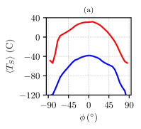
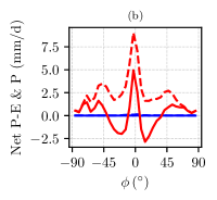
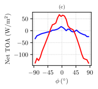
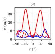
Figure 1: Climatological longitudinally averaged annual mean of (a) surface temperature, (b) Precipitation minus Evaporation (P-E, solid lines) and Precipitation (P, dashed lines), (c) top of the atmosphere net radiation, (d) magnitude of zonal wind speed at 300 hPa (solid lines) at 1000 hPa (near surface, dashed lines) versus the latitude $\phi$. Blue lines: SB state. Red lines: W state.

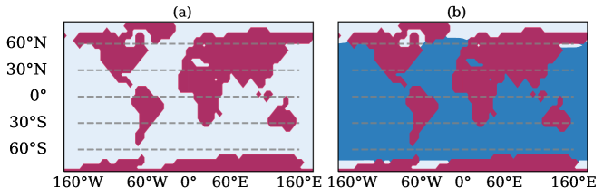
Figure 2: Sea-ice coverage comparison between (a) snowball and (b) warm climates, where the color coding is white for ice, blue for sea and red for land. We depict the land-map used by our model.

Fig. 1(a) shows the climatology of the zonal mean surface temperature. In agreement with previous studies performed on PLASIM (27; 8; 57), the SB state features global glaciation and extremely low temperatures at all latitudes, while the W state is similar to the present-day climate; see also the map of sea-ice cover in Fig. 2, where the limit of sea-ice approximately coincides with the isoline of $0^{\circ}$ C in the surface temperature shown in Fig. 1(a).

Figure 1(b) shows the annual mean budget of the precipitation minus evaporation rate (P-E) as well as the annual zonally averaged precipitation. The SB climate is almost entirely dry, as a result of the fact that the very low temperature of the atmosphere permits the presence of nothing but an extremely small amount of water vapour, because of the constraint posed by the Clausius-Clapeyron relation (1). The W climate has the familiar maximum of precipitation in the equatorial belt and secondary peaks in the mid-latitudes, resulting from convective precipitation and synoptic disturbances, respectively. The P-E field describes the scenario of net water vapour transport from the tropics into the equatorial belt and into the mid-latitudes (1).

Figure 1(c) shows the zonally averaged net TOA energy budget, which is the sum of the incoming shortwave radiation and the outcoming longwave radiation and scattered shortwave radiation. Note that the fluxes are positive when entering the planet and negative when leaving the planet. At steady state, the zonal TOA energy imbalance is compensated by the divergence of the meridional atmospheric enthalpy transport (1; 102; 103). We then conclude that such a transport is much stronger for the W state, where large contributions come from baroclinic eddies and from the large scale transport of water vapour. Baroclinic eddies are located in the region of the jet, where zonal winds in the upper troposphere at 300 hPa (near the tropopause, where the peak intensity is found) – Fig. 1(d) – and their existence is made possible by the conversion of available potential into kinetic energy via baroclinic instability, which is associated to the presence of a substantial meridional temperature difference between low and high latitudes in the atmosphere. The vigorous circulation of the W state corresponds to a powerful Lorenz energy cycle (105) ($\approx 3.4\text{W m}^{-2}$). Instead, the meridional enthalpy transport and the zonal circulation of the SB state are extremely weak, corresponding to the presence of very modest meridional temperature gradients (27; 8; 57). The SB state features a very weak Lorenz energy cycle ($\approx 1.0\text{W m}^{-2}$), as the presence of a weak meridional temperature gradient leads to a scarce reservoir of available potential energy and shuts down almost entirely the mechanism of baroclinic instability. The vast difference in the intensity of the Lorenz energy cycle in the two climates corresponds to the presence of much weaker surface winds in the SB than in W climate; see Fig. 1(d).

Table 1: Main climatic features of the stable climates for the two experimental configurations in absence of stochastic forcing ($\sigma=0$), where A refers to setup A, and B to setup B; W for warm state, C for cold state, and SB for snowball state; LEC stands for Lorenz energy cycle.

	$[\langle T_{S}\rangle]$ (∘C)	$\Delta T_{EP}$ (∘C)	sea ice (%)	LEC (W/m2)
A W	15.0(2)	26.4(3)	5.5(1)	3.39
A SB	-55.2(3)	25.7(5)	100	1.00
B W	4.4(3)	40.0(5)	27.7(1)	4.79
B C	-28(2)	53(1)	70(2)	3.79
B SB	-52.5(5)	25.9(5)	100	1.19

4.1.2 Noise-induced Transitions

In what follows, we will apply a very severe coarse-graining to the phase space of the model. Indeed, we perform a projection on the plane spanned by the globally and 30-day averaged surface temperature $[\langle T_{S}\rangle]$ and 30-day averaged Equator minus Poles surface temperature difference $\Delta T_{EP}=\langle T_{Eq}\rangle-\langle T_{Po}\rangle$, where we denote the spatial average of the field X by $[X]$, and the temporal average by $\langle X\rangle$. Specifically, $T_{Eq}=[T_{S}]_{30^{\circ}S}^{30^{\circ}N}$ and $T_{Po}\equiv\left([T_{S}]_{30^{\circ}N}^{90^{\circ}S}+[T_{S}]_{90^{\circ}S}^{30^{\circ}S}\right)/2$. Such a projection allows retaining a minimal yet still physically relevant description of the system (74; 29; 54; 49). Indeed, variations in the globally averaged surface temperature reflect, to a first approximation, changes in the energy budget of the planet (warming vs cooling), while $\Delta T_{EP}$ controls the large scale energy transport performed by the geophysical fluids (1; 103).

The asymptotic state of the system in absence of any form of stochastic forcing corresponds to either of the attractors described above and is determined by the initial condition. Transitions between the attractors can be induced by noise. In Fig. 3(a) we present the projection of the invariant measure of the stochastically forced system ($\sigma=18\%$) on the reduced phase space spanned by $[\langle T_{S}\rangle]$ and $\Delta T_{EP}$ (normalized to one), while Fig. 3(b) portrays the quasipotential estimated using Eqs. (3) and (7):

$$\Phi([\langle T_{S}\rangle],\Delta T_{EP})\sim-\frac{\sigma^{2}}{2}\log\rho_{\sigma}([\langle T_{S}\rangle],\Delta T_{EP}),$$ (9)

where the global minimum is set to 0. Note that the noise level given by $\sigma=18\%$ is the lowest allowing for a detailed global exploration of the phase space within a – for us – reasonably long (O($3\cdot 10^{4}$ $y$) simulation, as it allows for observing a good number (O(40)) of transitions between the $SB$ and the $W$ states. We find that the basin of the W attractor is deeper (lower values of the quasi-potential) compared to the basin of the SB attractor. By using Eq.(6) and performing an exponential fit of the statistics of average residence times in the two attractors for different values of the noise intensity – see Fig. 3(c), we obtain the following information on the two local potentials: $\Delta\Phi_{\rm W\rightarrow SB}\approx 700(40)$ and $\Delta\Phi_{\rm SB\rightarrow W}\approx 240(50)$. The good quality of the fit confirms that the weak-noise approximation is valid.

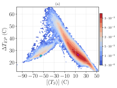
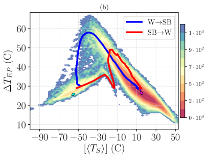
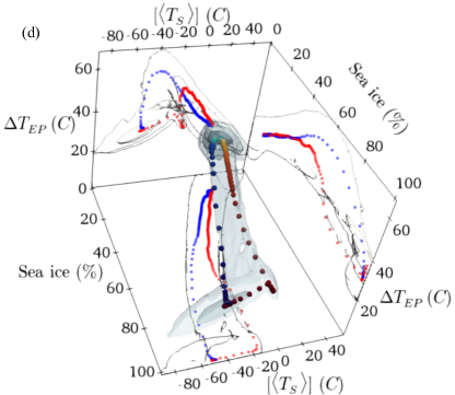
Figure 3: (a) Projection of the invariant measure on the reduced phase space spanned by the 30-day averaged global temperature $[\langle T_{S}\rangle]$ versus 30-day averaged Equator to pole temperature difference $\Delta T_{EP}$ for $\sigma=18\%$. (b) The corresponding quasipotential, shifted so that the global minimum is set to 0. The blue and red lines correspond to stochastically averaged transition paths for the W$\rightarrow$SB and SB$\rightarrow$W transitions. These trajectories follow different escape and relaxation paths, within each basin of attraction. The colored ellipses indicate the location of the deterministic attractors corresponding to SB state (cyan), and W state (magenta). (c) Average escape time versus the inverse squared $\%\sigma$, where dashed black and straight gray lines correspond to fitting Eq. (6). (d) Transition paths $\rm SB\rightarrow W$ (red) and $\rm W\rightarrow SB$ (blue) in the 3D space spanned by $[\langle T_{S}\rangle]$, $\Delta T_{EP}$, and the arctic sea ice percentage for $\sigma=18\%$. The shading indicates the density of the projected invariant measure, while a 2D projection of the transition paths in each plane is added. All data refer to setup A.

Another relevant piece of information can be obtained by looking at the paths of the $\rm SB\rightarrow W$ and $\rm W\rightarrow SB$ transitions. In the weak-noise limit, the stochastic average of the trajectories that manage to escape from either attractor gives the instantonic path for the portion of trajectory connecting the attractor to an M state, and the relaxation path for the remaining part of the trajectory, which connects the M state to the other attractor. The red (blue) line in Fig. 3(b) indicate the stochastic averages of the $\rm SB\rightarrow W$ ($\rm W\rightarrow SB$) transition trajectories. The procedure for computing the average paths is described in detail in the ESM.

As discussed above, escape trajectories and relaxation trajectories are expected to follow different paths in general nonequilibrium systems. We are indeed able to find such an essential feature of nonequilibrium systems, as clearly detailed in Fig. 3(b). In simpler setups with a unique saddle, the crossing point between the red and the blue line must correspond to the position of the M state, see discussion in (54; 49).

Instead, here the crossing between the two transition paths as observed in Fig. 3(b) is an artifact of looking at that specific two-dimensional projection, as can be noticed when looking at a three-dimensional projection of the phase space, see Fig. 3(d). The SB$\rightarrow$W and the W$\rightarrow$SB transitions go through two different channels corresponding to two different M states. This marks a major difference with respect to the analysis performed in (54; 49). We have clear indication that in the model used here large-scale currents are present in the phase space, which characterise non-equilibrium conditions; see (106) for an application of this concept in a climatic context.

It is reasonable to ascribe such a difference to the fact that here we are able to include a large class of processes associated with the transport of water and with its phase changes between solid, liquid, and gaseous forms. Indeed, the hydrological cycle is greatly responsible for the irreversibility of atmosphere (107; 108; 2) and, at more quantitative level, overwhelmingly contribute to the total entropy production of the geophysical fluids compared to the dissipation of kinetic energy and the turbulent exchange of sensible heat (109; 56; 57; 110). We argue that the lack of a comprehensive treatment of water in the model used in (54; 49) leads to an underestimation of the actual entropy production of the system, which makes it closer to equilibrium than the model considered here. According to a statistical mechanics angle, one sees this as associated with the absence (or significant reduction) of probability currents, which are largely suppressed by the presence of a single saddle separating the competing basins of attraction.

Phenomenologically, the presence of clear distinction between the SB$\rightarrow$W and the W$\rightarrow$SB transition paths explicitly indicates that the global thawing and the global freezing of the planet are fundamentally different processes. The thawing proceeds as follows. First, because of persistent positive anomalies of the solar irradiance, the global temperature of the planet grows without much changes in $\Delta T_{EP}$, as the atmospheric circulation is extremely weak and the oceanic transport absent. Then, the equatorial belt starts to melt and, due to the large decrease of the albedo in the equatorial band and subsequent intense warming, $\Delta T_{EP}$ increases substantially – see the almost vertical portion of the red line in Fig. 3(b). This leads to a strong enhancement of the meridional heat transport performed by the atmosphere and by the ocean, which causes the thawing of the sea-ice at higher latitudes until the sea-ice line reaches very high latitudes compatible with the W climate.

The global freezing of the planet, instead, proceeds in the following way. The cause of the freezing is, obviously, the presence of a (rare) persistent negative anomaly of the solar irradiance. The reduction of incoming solar radiation has an amplified effect at high latitudes, because of the ice-albedo feedback, leading to an increase of $\Delta T_{EP}$. The increase in $\Delta T_{EP}$ causes a strengthening in the meridional heat transport, which acts as a stabilizing feedback – see the diagonal portion of the blue line in Fig. 3(b). Nonetheless, if the anomaly in the solar irradiance is sufficiently strong and persistent, the sea-ice line moves equatorward, until the equatorial belt freezes and undergoes further extreme cooling because the albedo becomes very high, leading eventually to a very low value of $\Delta T_{EP}$ in the final SB state.

4.1.3 Relaxation Modes

As detailed in the ESM, by constructing a finite-state Markov chain model of the projected $([\langle T_{S}\rangle],\Delta T_{EP})$ space, one can extract further useful information about the slow dynamics of the system. We study the statistics of the transitions of the state of the system for the case $\sigma=18\%$ on a time scale of 30 days. The dominant eigenvector of the Markov chain is the projection of the invariant measure given in Fig. 3(a). The subdominant eigenvectors describes how a generic initial measure relaxes to the invariant one. We remark that, despite the very severe projection, the Markov chain model features positive metric entropy, which measures the rate of creation of information, and positive entropy production, which unequivocally indicates nonequilibrium conditions and is associated to the presence of currents (111).

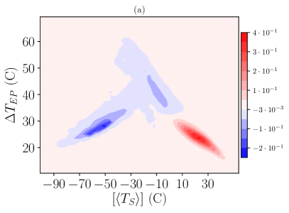
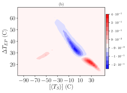
Figure 4: First two subdominant eigenvectors of the finite state projected Markov operator for setup A and $\sigma=18\%$. (a) First subdominant mode ($\tau\approx 30y$) describing the transitions between the two competing metastable states; see also a clear signature of persistent cold departures of the system – within the W basin of attraction – from typical warm conditions leading to the transitions. (b) Second subdominant mode ($\tau\approx 11y$) describing the low-frequency variability within the W basin of attraction. Note the lack of time-scale separation between these two modes.

The two leading subdominant eigenvectors of the finite-state Markov chain approximation of the projection of the transfer operator in the $([\langle T_{S}\rangle],\Delta T_{EP})$ plane for the case $\sigma=18\%$ are presented in Fig. 4. Panel (a) describes – in statistical terms – the coarse grained, slow process of transition between the two metastable states. One of two peaks is negative and the other one is positive, as the mode describes a zero-sum probability transfer. Additionally, this eigenvector has a very clear signature of persistent excursions of the system in the far cold region of the warm attractor. This might be interpreted as a signature of the preferential regions where transitions between the $SB$ and $W$ states take place, compare with Fig. 3(b).

Instead, panel (b) by and large describes the slowest intrawell variability, which takes place in the W basin of attraction: the two closely spaced peaks of opposite sign are on the opposite sides of the peak of the W basin of attraction, with the zero isoline cutting across the peak of the warm attractor; compare with Fig. 3(a). This slow time scale is associated with the process of ice formation and melting. A smaller peak is present in correspondence to the SB basin of attraction, indicating that this eigenvector captures some $\rm W\rightarrow SB$ escape process; compare with Fig. 3(b).

4.2 Setup B – Atmospheric-only Large Scale Energy Transport

4.2.1 The Three Competing Climate States

Excluding the large-scale heat oceanic transport amounts to removing a very powerful negative feedback, i.e. a mechanism of stabilization for the climate that efficiently redistributes energy throughout the system. This changes qualitatively the global stability properties of the system compared with the case of setup A. Indeed, in setup B we find three competing climate states, whose basic features are reported in Table 1, and we refer to Fig. 2 in the Supplementary Material for further evidence. One of the climates is the fully-glaciated SB state, which features very low $\Delta T_{EP}$ and extremely low global temperature, close to $-50~{}^{\circ}$C. The second climate resembles the W state found in setup A, featuring an above 0 ^∘C global temperature, with $\Delta T_{EP}\approx 40~{}^{\circ}$C and roughly 27% sea ice coverage. Between the two, lies the – unexpected and unprecedented for PLASIM – C state, which is not fully ice covered, and even though it has $[\langle T_{S}\rangle]\approx-30~{}^{\circ}$C, the fact that $\Delta T_{EP}\approx 50~{}^{\circ}$C suggests the presence of a warm latitudinal band at subtropical latitudes. The presence of an ice-free latitudinal band has huge implications in terms of habitability (24; 112).

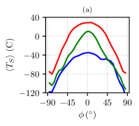
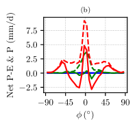
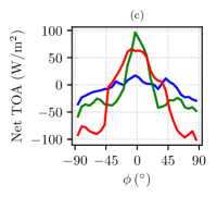
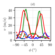
Figure 5: Climatological longitudinally averaged annual mean of (a) surface temperature, (b) Precipitation minus Evaporation (P-E, solid lines) and Precipitation (P, dashed lines), (c) top of the atmosphere net radiation, (d) magnitude of zonal wind speed at 300 hPa (solid line) and at 1000 hPa (near surface, dashed lines) versus the latitude $\phi$. Blue lines: SB state. Red lines: W state. Green lines: C state.

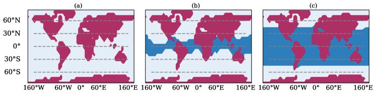
Figure 6: Sea-ice coverage comparison between (a) snowball, (b) cold and (c) warm climates. Note that the W state of setup B has more sea-ice than the W state of setup A.

In Fig. 5 we compare the climatology of the three climates (W in red, C in green and SB in blue) resulting from a 40-year average in steady state conditions, in absence of stochastic forcing ($\sigma=0$). The SB state is very similar to the one obtained with setup A, as the ocean plays a negligible role in a fully glaciated planet, and will not be further discussed here. The W state is similar with its counterpart in setup A, albeit considerably colder, and, correspondingly, with a weaker hydrological cycle. We can interpret this as resulting from the ice-albedo feedback. Indeed, the presence of a weaker heat transport towards high latitudes due to removing the oceanic channel of meridional transport leads to a larger sea-ice surface – compare Fig. 2(b) with Fig. 6(c) – which contributes to lowering the planetary albedo, thus enhancing the input in the energy channel at TOA. Due to the Boltzmann radiation feedback, the steady state must then be characterized by a lower average temperature compared to setup A. Finally, the presence of larger temperature differences between high and low latitudes lead to a stronger atmospheric variability, as baroclinic conversion is more efficient and can draw from a larger reservoir of available potential energy. This is associated with a stronger Lorenz energy cycle compared to setup A, see Table 1; see a discussion of the climatic effects of modulating the meridional oceanic heat transport in the W state in (104).

Fig. 5(a) shows the climatology of the zonal mean surface temperature. We remark that in the C state the subtropical band $[-20^{\circ}N,20^{\circ}N]$ features above-freezing temperature, while lower temperatures, and correspondingly, prevailing sea-ice is present at higher latitudes, as shown in Fig. 2. Despite PLASIM’s simplified dynamics, the C state shares features of the previously mentioned Slushball state (113) and, especially, of the Jormungand state (28), where the presence of ice-free equatorial band is associated with the dynamics of continental ice sheets and of the interplay of sea-ice cover, surface albedo, and atmospheric circulation, respectively. Figure 5(b) shows the annual mean budget of the precipitation minus evaporation rate (P-E; solid lines) as well as the annual zonally averaged precipitation (dashed lines). The C state features an intense precipitation in the equatorial belt, driven by the strong convection occurring there, but the P-E field indicates that the water vapour is recycled and no large scale transport takes place, as opposed to the W state.

Figure 5(c) shows the zonally averaged net TOA energy budget. One can infer that the meridional atmospheric enthalpy transport has comparable intensity in the W and C climates, yet the peaks of the transport – indicated by vanishing values of the TOA budget (1; 102; 103)- are confined to lower latitudes in the latter case. This indicates a vigorous heating realized at $\approx\pm 30^{o}N$. Correspondingly, the jet stream for the C state is located at lower latitudes compared to the W climate (panel d), while it is more intense, as the local meridional temperature gradient throughout the atmosphere is larger. This corresponds to a large temperature difference between low and high latitudes at surface, see Table 1.

Finally, the C state features a strong Lorenz energy cycle ($\approx 4.0\rm Wm^{-2}$), thanks to the presence of such large meridional temperature gradients which correspond to a large reservoir of available potential energy that can be converted to kinetic energy by baroclinic instability. The intensity of the Lorenz energy cycle of the C state is especially remarkable given that the atmospheric circulation is relatively weak poleward of $50^{\circ}$ latitude.

4.2.2 Noise-induced Transitions

The presence of three instead of two deterministic attractors makes setup B considerably more complex than setup A; for example now the existence of extra M states connecting SB with C and W with C has to be taken into account, on top of those connecting SB with W already seen in setup A. Figure 7(a) shows the projection of the invariant measure in the reduced phase space given by $([\langle T_{S}\rangle],\Delta T_{EP})$ obtained for $\sigma=12\%$, while in Fig. 7(b) we show the corresponding estimate of the quasipotential. We remark that in setup B a lower noise intensity is needed to excite transitions with frequency comparable to what obtained in setup A, for the basic reason that we are missing the global stabilizing feedback given by the ocean heat transport. This corresponds to having weaker diffusion in the Fokker-Planck operator describing the evolution of probabilities. The location of the deterministic attractors is shown with ellipses of different color, where magenta, green and cyan correspond to W, C and SB climate states, respectively.

The location of the C state is not directly visible in the projected invariant measure or in the quasi-potential, in the form of a local maximum and minimum, respectively. The operation of performing a projection to such a low-dimensional space is mainly responsible for such a loss of information. This issue is addressed specifically in Sec. 4.3. Additionally, as we shall see below, the third attractor corresponds to a much shallower local minimum of the quasi-potential compared to the W or SB states. As a result, the C local minimum is washed out when considering a noise intensity of $\sigma=12\%$, and it is hard to keep track of orbits persisting significantly near C, see Eqs. (3)-(6). This implies the presence of an additional scale relevant for understanding the multistability of the system, along the lines of what depicted in Fig. 12.

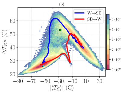
Figure 7: (a) Projection of the invariant measure of the system in the reduced phase space composed of the 30-day averaged global temperature versus 30-day averaged Equator to pole temperature difference for setup B and $\sigma=12\%$. The stochastically averaged escapes from the C state with $\sigma=6\%$ are also included. (b) The corresponding quasipotential, shifted so that the global minimum is set to 0. The blue and red lines correspond to stochastically averaged transition paths for the W$\rightarrow$SB and SB$\rightarrow$W transitions. The trajectories are completely different, depending on the direction of the transition. The ellipses indicate the location of the deterministic attractors corresponding to the SB state (cyan), the C state (green) and the W state (magenta).

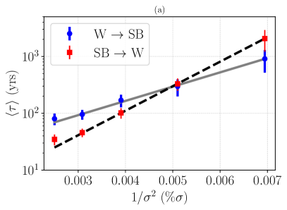
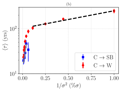
Figure 8: Average escape time versus the inverse squared $\%\sigma$ in setup B. (a) Comparison of W$\rightarrow$SB (filled blue circles) and SB$\rightarrow$W (filled red squares) and corresponding exponential fit, gray straight and black dashed lines. (b) Comparison of C$\rightarrow$SB (filled blue squares) and C$\rightarrow$W (filled red circles) and corresponding exponential fit, gray straight and black dashed lines. The fitting expression is given by Eq. (6).

As mentioned above, the presence of ocean diffusion triggers the ice-albedo feedback in a direction that favours warming. Accordingly, in setup B, the minimum of the quasipotential corresponding to the SB state is deeper than the one corresponding to the W state. This can be seen in Fig. 8(a), where the $SB\leftrightarrow W$ mean escapes times $\bar{\tau}_{\sigma}$ are presented as a function of the inverse squared noise amplitude. Using Eq.(6), we obtain the following estimates for the depth of the local quasi-potentials: $\Delta\Phi_{\rm W\rightarrow SB}\approx 290(10)$ and $\Delta\Phi_{\rm SB\rightarrow W}\approx 500(10)$. As opposed to setup A, in setup B the pre-exponential factors of the expectation value of escape times is vastly different. Note that, neglecting the C state, the population of the SB and W state is inversely proportional to the corresponding escape times. As a result, despite being associated to a shallower local minimum of the quasi-potential, the fraction of population in the W state is larger when considering relatively strong noise intensity, whereas eventually, the SB state dominates in the weak-noise limit. Despite the profound dynamical differences between setup A and B, the estimates of the instantonic and relaxation paths between the SB state and the W state are qualitatively similar; compare Figs.3(b) and 7(b). Furthermore, the interpretation of the different physical mechanisms controlling the SB$\rightarrow$W and W$\rightarrow$SB transitions paths for setup B is fundamentally the same as for setup A.

The more complex geometry of the phase space of setup B is made apparent by the fact that (see the movies included in the ESM), the transitions between the W and SB states can be either direct or, instead, the paths deviate considerably as the orbit is temporarily trapped near the C state. Such a trapping is always extremely short-lived compared to the other relevant time scales associated with the transition between the two other metastable states.

The next step is to provide a characterization of the quasi-potential near the C state, and, specifically, to estimate the C$\rightarrow$SB and C$\rightarrow$W barriers for the local quasi-potential. Following (54), we investigate the escape process from the C state by considering a large number of trajectories initialized in the deterministic C attractor and apply a weaker random forcing with $\sigma=(1\%-10\%)$. We then collect the statistics of escape times and keep a separate track for trajectories ending up in the W versus in the SB state through the corresponding M states. Using Eq. (6), we are able to estimate the two quasi-potential barriers $\Delta\Phi_{\rm C\rightarrow SB}$ and $\Delta\Phi_{\rm C\rightarrow W}$. We see in Fig. 8(b) that $\Delta\Phi_{\rm C\rightarrow SB}\approx 16(2)$ (blue filled squares) is about one order of magnitude smaller than the W$\leftrightarrow$SB barriers. Interestingly, the energy barrier $\Delta\Phi_{\rm C\rightarrow W}\approx 0.45(4)$ (red filled circles) turns out to be much smaller than $\Delta\Phi_{\rm C\rightarrow SB}$, which explains why bellow a certain noise level, i.e. $\sigma\approx 4\%$ we practically get no transitions towards the SB attractor, with all escape trajectories ending in the W basin of attraction. Also, for the C$\rightarrow$W transitions, we clearly observe from Fig. 8(b) that for $\sigma$ larger than $\sigma\approx 5\%$ there is a different scaling that can be attributed to the prefactor in Eq. (6), which indicates that the weak-noise limit is not achieved for these values of $\sigma$ for these escape processes. Further comments on the escape from the C state can be found in the ESM.

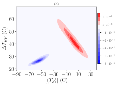
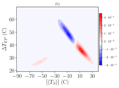
Figure 9: First two subdominant eigenvectors of the finite state projected Markov operator for setup B and $\sigma=12\%$. (a) First subdominant mode ($\tau\approx 290y$) describing the transitions between the two main competing metastable states. (b) Second subdominant mode ($\tau\approx 10y$) describing the low-frequency variability within the warm attractor. Note the lack of any signature of the cold attractor, whose lifetime is much shorter than 10 years at noise level $\sigma=12\%$.

4.2.3 Relaxation Modes

Finally, we study the two subdominant eigenvectors of the finite-state Markov chain approximation of the projection of the transfer operator in the $([\langle T_{S}\rangle],\Delta T_{EP})$ plane for the case $\sigma=12\%$, see Fig. 9. As in setup A, the Markov chain model features positive metric entropy and positive entropy production. We get a broad agreement with the results of setup A also in terms of interpretation of the meaning of the eigenvectors, but a more clear separation of scales between the two corresponding eigenvalues is evident in this case. In Fig. 9(a) the first subdominant eigenvector has a much longer life-time of approximately 290 years, which matches the life time of the SB state. Because of such a long time scale, and of the fact that the transition time is very short compared to the residence time, we lose any feature of the transition path, as opposed to setup A. The eigenvector shown in Fig. 9(b) has a life-time of about 10 years and portrays the low-frequency variability in the W basin of attraction, which can lead to occasional transitions towards the SB state; compare the $\rm W\rightarrow SB$ transition path in Fig. 7(b). We find no signature of the presence of the C state, whose life time is much smaller than 10 years for this level of noise. These eigenvectors further clarify that for this level of noise the C state is almost entirely washed out.

4.3 Automatic determination of the metastable states

The basic issue we want to address now is that, while in Fig. 7 the SB and W state clearly appear as corresponding to local maxima of the projected invariant measure, this is not the case for the C state, in this as well as in many other 2D projections we have tested. Indeed, it has been impossible with the tools developed so far to find any direct evidence of the C state in the stochastic integrations. As described in Sect. 4.2.1, the discovery of the C state has been serendipitous and based on the exploration of the phase space via forward deterministic simulations. We next show what can be obtained by applying the suite of data driven methods (66; 67; 69) presented in Section 2.2 to the output of some given numerical simulations taken as pseudo-observations of an in principle unknown model.

We first consider a numerical integration of the model in setup B lasting $6\cdot 10^{4}$ years and performed with $\sigma=12\%$. From the complete trajectory of $O(10^{5})$ d.o.f. recorded with having temporal resolution of one time step, we construct a severely coarse-grained version of the phase space by a set of 30-day averaged air temperatures measured every 10 months (hence, decimated with respect to the standard 30-day averaged dataset in previous sections) at three different pressures (300, 500 and 1000 hPa) and 32 different latitudes, for a total of $n=96$ variables. The quasipotential as a function of these variables is, in principle, a 96-dimensional function, which cannot be visualized or estimated in a simple manner.

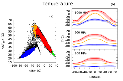
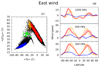
Figure 10: The topography of the quasipotential in high-dimensional spaces. Panel (a) and (b): the analysis is performed for setup B and $\sigma=12\%$ in the coordinate space of the air temperature at three different pressures (300, 500 and 1000 hPa) at 32 latitudes between -86^o and 86 ^o (96 variables). Panel (c) and (d): the analysis is performed on the time series of the zonal and the meridional wind in the same latitudes and pressures (192 variables). Panel (a) and (c) portray the estimated basins of attraction of the quasipotential, which are represented in the $([\langle T_{S}\rangle],\Delta T_{EP})$ projection. The core sets of each attractor are colored in blue (SB state), orange (C state) and red (W state). The green points are the core set of spurious attractors found by the algorithms in both setups. The black points are configurations which do not belong to any core state. Panel (b) and (d) portray the average value plus/minus one standard deviation of the variables, restricted to the core sets of the SB (blue), W (red) and C (orange) states, as light shaded area. In comparison, the time averages of the same variables, computed for the corresponding deterministic attractors, is shown in dark solid lines of the same color, respectively. The meridional wind is not shown.

By using the approach outlined in Sec. 2.2, we study the topography of this function. We first estimate the intrinsic dimension of the manifold containing the data, which turns out to be $\sim 11$, significantly smaller than the number of variables . This number is approximately scale invariant: indeed the estimated value does not change significantly if the data set is significantly undersampled. Since the intrinsic dimension of the embedding manifold is relatively low and well-defined, one can estimate the quasipotential $\Phi_{t}$ in each time frame $t$ using Eq. (8), without defining explicitly the $\sim$ 11 coordinates mapping the manifold. Using these estimates, one finds the attractors, which correspond to the local minima of $\Phi$. With a statistical confidence level of 99%, corresponding to $Z=2.576$, we find 4 states, with a core population of 39171, 12099, 112 and 11 frames respectively. The configurations corresponding to the four minima of $\Phi$ were then evolved without stochastic forcing in order to obtain the corresponding asymptotic states, While the first three states are in the basin of attraction of the SB, W, and C attractors, correspondingly, the fourth state is found to be unstable, as it forward evolution converges to the W attractor. This indicates that the fourth state is an artifact of finite sampling, or of the variations of the $Z(x)$ (see Eq. (3)) which in the estimate of $\Phi_{t}$ are neglected. The configurations assigned to the core set of the three remaining states are represented in Fig. 10(a) in the same projection used in Fig. 7. In this projection the C and W states strongly overlap, and no barrier is visible between the two.

In Fig. 10(b) we plot the average and the standard deviation, estimated for the core set of each state, of the 96 air temperature variables used in the analysis. Note that such average values agree remarkably well with the time-averages one obtains by considering the corresponding deterministic attractors, represented as continuous lines in Figure 10. Remarkably, the distributions are significantly well separated for almost all the variables. This demonstrates that the W and C state are indeed non-overlapping in the 96-dimensional space of these variables. This also shows that the data-driven approach presented here is able to reconstruct accurately the statistical properties of the competing deterministic metastable states.

We then repeated the exercise by considering the $n=192$ variables describing the 30-day averaged meridional and zonal wind at the same latitudes and pressure levels as before. The intrinsic dimension of this dataset is $\sim 16$, slightly larger than for the other variables. In this space, at a statistical confidence of $99\%$ the algorithm is able to detect only two states, the W and the SB states. At a $98\%$ confidence the C states appears (orange points in Fig. 10(c)), together with another state, represented in green. The latter state turns out to be spurious, since simulations performed with $\sigma=0$ starting from the estimated minimum rapidly converge to the SB state. In this space the C state is much more similar to the W state, as illustrated in Fig. 10(d): the average zonal wind differs significantly only in the mid-latitudes of the Southern Hemisphere at all levels and in the mid-latitudes of the Northern Hemisphere only at 500 hPa. Note also in this case the excellent agreement obtained with the average statistics computed for the corresponding deterministic attractors.

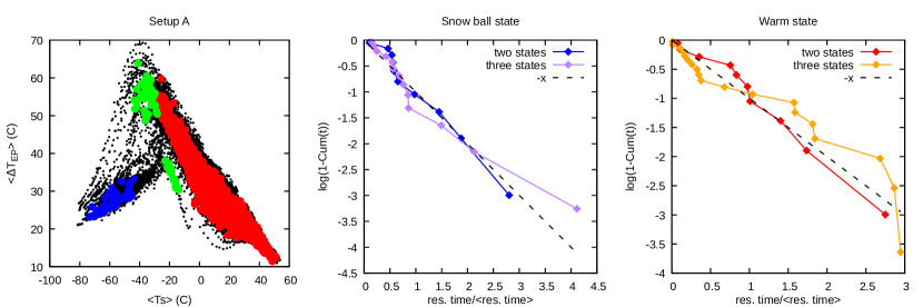
Figure 11: The quasipotential and the residence times for setup A and $\sigma=18\%$. Panel (a): the states obtained analyzing the coordinate space of the air temperatures at three different pressures at 32 latitudes (the same variables used in the analysis in Fig. 10-a). The analysis is performed with Z=5. At higher statistical significance the green state disappears. Panel (b) and (c): the empirical cumulative distribution $C(x)$ of the normalized escape time $x=t_{\text{esc}}/<t_{\text{esc}}>$, where $<t_{\text{esc}}>$ is the average of all the observations. Panel (b): the SB state. Panel (c): the W state. Blue and red lines: the green state in panel a is not considered meaningful. Purple and orange lines: the green state is considered meaningful. The dashed black lines correspond to the ideal case in which $x\sim\exp(-x)$, and therefore $\log(1-C(x))=-x$.

We also performed the same analysis on a simulation evolved for 32780 years using the model in setup A and with $\sigma=18\%$. At high statistical significance, we detect two states corresponding to the W and the SB climates, described in Sect. 4.2.1. At lower statistical significance other states appear. An example of an analysis is shown in Fig. 11(a), where the green state approximately seem to occupy approximately the same region as the C state found in setup B, see Fig. 10(a). However, the distribution of the air temperature variables in this state differs significantly from the C state in setup B (not shown). Indeed, this state is not an attractor, as it evolves towards the W state if one removes the stochastic forcing. rapidly to the W state. The dynamics of an ensemble of trajectories initiated near the green dots is by and large controlled by two subdominant eigenvectors depicted in Fig. 4(a-b).

These results indicate that our approach allows identifying the correct metastable states of a complex high-dimensional dynamic model, but these states come with an uncertainty, which partially derives from statistical errors, and partially from the approximations intrinsic in the quasipotential estimator, which neglects the preexponential factor $Z(x)$. Finally, an error is introduced by the correlation between the frames, which are generated by a dynamic model and sampled with a time lag of a few months. However, one can rather straightforwardly recognize the spurious states, even without performing a simulation at $\sigma=0$, by estimating, on the same trajectories which brings to their identification, the probability distribution of the first escape times. This distribution is estimated by assuming that the system performs a transition between two states when it visits a core configuration belonging to a state which is different from the state of the last core configuration visited in the past (114). In this manner, one splits the trajectory in segments, each labeled with a different state, whose length is an estimate of the escape time $t_{\text{esc}}$. If the set of states defines (at least approximately) a Markov model, $t_{\text{esc}}$ should be exponentially distributed. In Figs. 11(b-c) we plot a function of the empirical cumulative probability distribution of $t_{\text{esc}}$ which, if $t_{\text{esc}}\sim\mathrm{Exp}$, should coincide with the black dashed lines. If one considers as meaningful also the green state in Fig. 11(a) one obtains a set of $t_{\text{esc}}$ from the W and the SB state whose distribution significantly deviates from an exponential (purple and orange lines in panels b and c). If instead one does not consider the green state as meaningful, the distribution of the escape times from the W and SB state is almost perfectly exponential (blue and red lines), as far as one can judge from the relatively small number of transition events observed in the trajectory. This analysis indicates that our approach allows identifying the correct metastable states of the system even from relatively short trajectories, in which only $\mathcal{O}(10)$ transitions are observed. The states can be identified in a fully unsupervised manner, analyzing only the trajectory or by running short relaxation dynamics with $\sigma=0$.

5 Conclusions

Achieving a deeper understanding of the nature of the Earth’s multistability and related tipping points is one of the key contemporary challenges because it is essential for better framing the co-evolution of climatic conditions and of the biosphere throughout the Earth’s history, and, in the present context, for better constraining the current planetary boundaries through a careful examination of the safe operating space for Humanity (115).

Systems undergoing stochastic dynamics and featuring competing multistable states can be effectively described by taking advantage of the formalism of the quasi-potential landscape, which generalizes the notion of the free energy to nonequilibrium systems. Local minima in the quasipotential describe competing metastable states, and are separated by local maxima and saddles – M states – that define possible gateways for transitions. To demonstrate our framework in the case of the climate we employ two versions of an open source climate model, PLASIM, which has an appropriate mix of precision, flexibility, and efficiency in simulating the present climate as well as very exotic climatic conditions. The first version (setup A) features a simplified but meaningful representation of the oceanic energy transport from low to high latitudes, whereas in the second one (setup B) large scale energy transport is provided solely by the turbulent atmosphere. Setup A demonstrates the well-known competing climatic states corresponding to the present warm (W) conditions and the so-called snowball (SB) climate. Setup B, instead, contains an unexpected additional intermediate stable climate (C) where the sea is partially ice-free in the equatorial band. The lack of a powerful mechanism of energy redistribution across the climate makes this additional state possible. Despite PLASIM’s relative simplicity, the C state should not be regarded as a pure mathematical curiosity corresponding to a pathological solution: exotic climate states rather similar to the C state obtained here have been obtained in other climate models and are deemed extremely relevant in paleoclimatic terms because they provide a scenario able to explain the survival of life during the Neoproterozoic glaciations.

The phase space of the model can be explored when stochastic forcing – here in the form of a yearly fluctuating solar irradiance – is introduced, leading to transitions between the competing metastable states. We compute the quasipotential function, which describes, on the one side, the invariant measure of the system and, on the other side, in its local version, controls the probability of transition of the stochastically forced trajectory from one to another basin of attraction. We are able to estimate in both setups the optimal escape paths – the instantons – and the corresponding relaxation trajectories linking the W and SB states, and are then able to verify the nonequivalence between the two, which is an essential feature of nonequilibrium properties.

Instantons describe how transitions take place in the zero-noise limit and are more of a mathematically elegant construction than a physically relevant object in our investigations, as we need to consider noise of moderate yet non-negligible intensity in order to observe reasonably frequent transitions between the SB and W attractors. Additionally, studying the transfer operator in a suitably projected space sheds light on how the system relaxes to its invariant measure. We are able to find clear evidence of both interwell relaxation processes, which describe transitions between competing metastable states, and are the noisy version of instantons, and intrawell relaxation processes, which would conventionally be labelled as ultralow frequency variability within the W state associated with large scale melting and thawing of sea ice and corresponding large temperature fluctuations.

A nontrivial result we obtain is that the instantons escaping the SB and the W attractors do not meet at one of the M states separating the two corresponding basins of attraction. This can be best appreciated visually by watching the videos included in the ESM. In fact, the transitions take place through two separate saddles. This has two important implications a) the dynamics on the basin boundary is, by itself, multistable; and b) one has large-scale nonvanishing currents in the phase space. This is a strong signature of the nonequilibrium nature of the system. The existence of separate paths for the SB-to-W and W-to-SB states marks a relevant difference with previous studies. The presence of more evident macroscopic signature of nonequilibrium conditions can be attributed to the presence in this model of an active hydrological cycle, which is the major agent of entropy production in the climate system.

The C state in setup B corresponds to a comparably shallower minimum of the quasipotential, which can be explored only considering significantly weaker noise than needed to explore globally the phase space of the system. We discover that the most natural, preferential escape route from the C state is towards the W state. The C state is only barely metastable, as even internally generated noise of the numerical discretization can destabilize it, even if only rarely and over ultra long time scales. The position in phase space of the C state and its properties indicate that it is likely that the C state is the leftover of the M state between the SB and W climate obtained as we progressively switch off the horizontal diffusivity of the ocean, because this leads to a less efficient redistribution of energy in the system,

We have complemented the top-down approach based on numerical modelling with bottom-up data-driven methods that allow for the automatic detection of the competing metastable states from the analysis of a single long stochastic trajectory and to reconstruct the quasi-potential in arbitrarily high-dimension. Using this approach we have been able to reconstruct the dynamical landscape of the climate model in both setups and gain a better understanding of how transitions between the competing metastable states occur. Remarkably, by suitable averaging over many realizations, we have been able to reconstruct the climates of the competing (deterministic) metastable states.

5.1 Outlook: Multiscale Multistability

The quasipotential landscape viewpoint might provide a useful way for describing the multistability of the climate in a hierarchical fashion. We present in Fig. 12(a) an illustration of this perspective, where the possible states of the climate are described by the vector $X$. The quasi-potential $\Phi$ features troughs, saddles, and ridges at different scales.

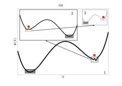
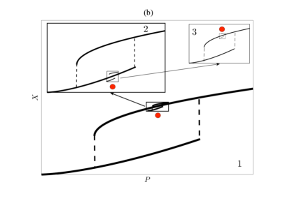
Figure 12: Schematic representation of the multiscale nature of multistability in the climate system. (a) Quasipotential $\Phi$ as a function of the state of the system $X$. (b) Corresponding hysteresis loops as a function of a parameter $P$. The white boxes indicate the zoomed-in current state of the system (red dot), going from 1 to 3 towards smaller and smaller scales.

The intensity of noise allowing for exploring transitions between competing states decreases dramatically as we go from level 1 to level 3, because the local minima become shallower. Going to even smaller scales, one would find additional (shallower) corrugations of $\Phi$. Multistability in the climate system is often revealed by the presence of hysteresis loops obtained when suitable parameters of the system are changed, usually quasi-adiabatically (32; 116; 27). Figure 12(b) shows schematically how the multistability portrayed in Fig. 12(a) appears when applying suitable protocols of parametric modulations to the system.

The above description could potentially be a fundamental mathematical structure linking the global multistability of the climate system with the geographically localized tipping elements and the so-called cascading tipping points, and might be useful for understanding the associated multiscale hysteretic behaviour of the climate system when parameters are suitably modulated. We stress that in the current work we have been able to explore only the highest hierarchical level of multistability. A more complete model and a suitable, different choice of stochastic forcing would be needed for exploring the small scale local minima of the quasipotential associated, e.g., with competing climate states that exchange stability at tipping points like the ocean associated with the AMOC shutdown. In this case, one would need a model able to resolve explicitly the deep ocean circulation and possibly consider random perturbations to the hydrological cycle acting in the North Atlantic sector.

We envision the combination of the top-down and bottom-up approach as a possible way forward to study the multiscale nature of the multistability of the climate system, as well as of other systems of comparable complexity. This research work paves the way for further investigation into some fundamental properties of the climate system and goes in the direction of clarifying its intransitive vs quasitransitive vs transitive nature (117) when different time scales are considered. Additionally, it indicates a way for fostering the development of climate models of different level of complexity: indeed, we want them to be able to capture the qualitative features of climate, by allowing for the presence of a complex dynamical landscape featuring hierarchically arranged – according to the desired level of envisaged detail and granularity – competing metastable states, associated with the ensuing tipping points.

The viewpoint presented here seems also promising for investigating a separate, extremely relevant aspect of atmospheric dynamics, namely the existence in the atmosphere of different regimes of operation, which define the presence of substantial low-frequency variability on subseasonal time scales (118; 4). This boils down to the fact that, at coarse-grained level, due to extreme dynamical heterogeneity (119), one is practically looking at a multistable system, where one can define and detect transitions between different metastable states (120).

Finally, we remark that white Gaussian noise might not necessarily be the only suitable way to treat stochasticity in the climate system (121). The theory of escapes from attractors in the presence of Lévy noise has been developed (122; 123) and very recently applied to simple geophysical models (124). It is well known that the mechanisms of escape are rather different than in the standard Gaussian scenario pursued in this paper. It seems then of great relevance to consider the effect of Lévy noise forcing in a more complex climate model like the one considered here.

The data required to generate the figures can be accessed via this repository: here. Animations presenting examples of transitions are publicly available on the youtube.com platform through the links that can be found in the text that can be found at here.

GM performed the simulations, contributed to the data analysis and to the writing of the paper. TG contributed to the writing of the paper. AL contributed to the data analysis and to the writing of the paper. VL proposed the research topic, contributed to the interpretation of the data analysis and led the writing of the paper. All authors gave final approval for publication and agree to be held accountable for the work performed therein.

The authors declare no competing interests.

TG acknowledges the support received from the EPSRC project EP/T011866/1. VL acknowledges the support received from the EPSRC project EP/T018178/1. VL and GM acknowledge the support received from the EU Horizon 2020 project TiPES (Grant no. 820970).

VL wishes to thank T. Bódai, N. Boers, M. Ghil, F. Lunkeit, G. Pavliotis, A. Tantet, and N. Zagli for many inspiring conversations on multistability and tipping points. GM wishes to thank F. Lunkeit for his guidance on PLASIM and kind hospitality at the University of Hamburg.

References

- (1) Peixoto JP, Oort AH. 1992 Physics of Climate. New York: AIP Press, New York.
- (2) Lucarini V, Blender R, Herbert C, Ragone F, Pascale S, Wouters J. 2014a Mathematical and physical ideas for climate science. Rev. Geophys. 52, 809–859.
- (3) Ghil M. 2015 A mathematical theory of climate sensitivity or, How to deal with both anthropogenic forcing and natural variability?. In P. CC, M. G, M. L, M. WJ, editors, Climate Change : Multidecadal and Beyond pp. 31–51. World Scientific Publishing Co./Imperial College Press.
- (4) Ghil M, Lucarini V. 2020 The physics of climate variability and climate change. Rev. Mod. Phys. 92, 035002.
- (5) Schneider SH, Dickinson RE. 1974 Climate modeling. Reviews of Geophysics 12, 447–493.
- (6) Saltzman B. 2001 Dynamical Paleoclimatology: Generalized Theory of Global Climate Change. New York: Academic Press New York.
- (7) Held IM. 2005 The gap between simulation and understanding in climate modeling. Bulletin of the American Meteorological Society 86, 1609–1614.
- (8) Lucarini V. 2013 Modeling complexity: the case of climate science. In Gohde U, Hartmann S, Wolf J, editors, Models, Simulations, and the Reduction of Complexity pp. 229–254. De Gruyter.
- (9) Budyko MI. 1969 The effect of solar radiation variations on the climate of the Earth. Tellus 21, 611–619.
- (10) Sellers WD. 1969 A global climatic model based on the energy balance of the earth-atmosphere system. Journal of Applied Meteorology 8, 392–400.
- (11) Ghil M. 1976 Climate Stability for a Sellers-Type Model. Journal of the Atmospheric Sciences 33, 3–20.
- (12) Stommel H. 1961 Thermohaline convection with two stable regimes of flow. Tellus 2, 244–230.
- (13) Veronis G. 1963 An analysis of the wind-driven ocean circulation with a limited number of Fourier components. Journal of Atmospheric Sciences 20, 577–593.
- (14) Rooth C. 1982 Hydrology and ocean circulation. Progress in Oceanography 11, 131–149.
- (15) Charney JG, DeVore JG. 1979 Multiple flow equilibria in the atmosphere and blocking. J. Atmos. Sci. 36, 1205–1216.
- (16) Lorenz EN. 1984 Irregularity: a Fundamental Property of the Atmosphere. Tellus A: Dynamic Meteorology and Oceanography 36, 98–110.
- (17) Lorenz EN. 1996 Predictability - a problem partly solved. In Palmer T, Hagedorn R, editors, Predictability of Weather and Climate pp. 40–58. Cambridge University Press.
- (18) Marshall J, Molteni F. 1993 Toward a Dynamical Understanding of Planetary-Scale Flow Regimes. Journal of the Atmospheric Sciences 50, 1792–1818.
- (19) Fraedrich K, Kirk E, Lunkeit F. 1998 Portable university model of the atmosphere.. Technical Report 16 Deutsches Klimarechenzentrum.
- (20) Petoukhov V, Ganopolski A, Brovkin V, Claussen M, Eliseev A, Kubatzki C, Rahmstorf S. 2000 CLIMBER-2: a climate system model of intermediate complexity. Part I: model description and performance for present climate. Climate Dynamics 16, 1–17.
- (21) Montoya M, Griesel A, Levermann A, Mignot J, Hofmann M, Ganopolski A, Rahmstorf S. 2005 The earth system model of intermediate complexity CLIMBER-3. Part I: description and performance for present-day conditions. Climate Dynamics 25, 237–263.
- (22) Stocker TF, Qin D, Plattner GK, Tignor M, Allen SK, Boschung J, Nauels A, Xia Y, Bex V, Midgley PM et al.. 2013 Climate change 2013: The physical science basis. Contribution of working group I to the fifth assessment report of the intergovernmental panel on climate change 1535.
- (23) Berner J, Achatz U, Batté L, Bengtsson L, Cámara Adl, Christensen HM, Colangeli M, Coleman DRB, Crommelin D, Dolaptchiev SI, Franzke CLE, Friederichs P, Imkeller P, Järvinen H, Juricke S, Kitsios V, Lott F, Lucarini V, Mahajan S, Palmer TN, Penland C, Sakradzija M, von Storch JS, Weisheimer A, Weniger M, Williams PD, Yano JI. 2017 Stochastic Parameterization: Toward a New View of Weather and Climate Models. Bulletin of the American Meteorological Society 98, 565–588.
- (24) Pierrehumbert R, Abbot D, Voigt A, Koll D. 2011 Climate of the Neoproterozoic. Annual Review of Earth and Planetary Sciences 39, 417–460.
- (25) Hoffman PF, Kaufman AJ, Halverson GP, Schrag DP. 1998 A Neoproterozoic Snowball Earth. Science 281, 1342–1346.
- (26) Lewis JP, Weaver AJ, Eby M. 2007 Snowball versus slushball Earth: Dynamic versus nondynamic sea ice?. Journal of Geophysical Research: Oceans 112.
- (27) Lucarini V, Fraedrich K, Lunkeit F. 2010 Thermodynamic analysis of snowball Earth hysteresis experiment: Efficiency, entropy production and irreversibility. Quarterly Journal of the Royal Meteorological Society 136, 2–11.
- (28) Abbot DS, Voigt A, Koll D. 2011 The Jormungand global climate state and implications for Neoproterozoic glaciations. Journal of Geophysical Research: Atmospheres 116.
- (29) Lucarini V, Bódai T. 2017 Edge states in the climate system: exploring global instabilities and critical transitions. Nonlinearity 30, R32–R66.
- (30) Lenton TM, Held H, Kriegler E, Hall JW, Lucht W, Rahmstorf S, Schellnhuber HJ. 2008 Tipping elements in the Earth’s climate system. Proceedings of the national Academy of Sciences 105, 1786–1793.
- (31) Boers N, Marwan N, Barbosa HMJ, Kurths J. 2017 A deforestation-induced tipping point for the South American monsoon system. Scientific Reports 7, 41489.
- (32) Rahmstorf S, Crucifix M, Ganopolski A, Goosse H, Kamenkovich I, Knutti R, Lohmann G, Marsh R, Mysak LA, Wang Z, Weaver AJ. 2005 Thermohaline circulation hysteresis: A model intercomparison. Geophysical Research Letters 32.
- (33) Walter KM, Zimov SA, Chanton JP, Verbyla D, Chapin FS. 2006 Methane bubbling from Siberian thaw lakes as a positive feedback to climate warming. Nature 443, 71–75.
- (34) Levermann A, Schewe J, Petoukhov V, Held H. 2009 Basic mechanism for abrupt monsoon transitions. Proceedings of the National Academy of Sciences 106, 20572–20577.
- (35) Steffen W, Rockström J, Richardson K, Lenton TM, Folke C, Liverman D, Summerhayes CP, Barnosky AD, Cornell SE, Crucifix M, Donges JF, Fetzer I, Lade SJ, Scheffer M, Winkelmann R, Schellnhuber HJ. 2018 Trajectories of the Earth System in the Anthropocene. Proceedings of the National Academy of Sciences 115, 8252–8259.
- (36) Klose AK, Karle V, Winkelmann R, Donges JF. 2020 Emergence of cascading dynamics in interacting tipping elements of ecology and climate. Royal Society Open Science 7, 200599.
- (37) Gammaitoni L, Hänggi P, Jung P, Marchesoni F. 1998 Stochastic resonance. Reviews of Modern Physics 70, 223–287.
- (38) Lucarini V. 2019 Stochastic resonance for nonequilibrium systems. Phys. Rev. E 100, 062124.
- (39) Benzi R, Sutera A, Vulpiani A. 1981 The mechanism of stochastic resonance. Journal of Physics A: Mathematical and General 14, L453–L457.
- (40) Nicolis C. 1982 Stochastic aspects of climatic transitions‚Äìresponse to a periodic forcing. Tellus 34, 308–308.
- (41) Ditlevsen PD. 2010 Extension of stochastic resonance in the dynamics of ice ages. Chemical Physics 375, 403 – 409.
- (42) Alley RB, Anandakrishnan S, Jung P. 2001 Stochastic resonance in the North Atlantic. Paleoceanography 16, 190–198.
- (43) Ganopolski A, Rahmstorf S. 2002 Abrupt Glacial Climate Changes due to Stochastic Resonance. Phys. Rev. Lett. 88, 038501.
- (44) Vélez-Belchí P, Alvarez A, Colet P, Tintore J, Haney RL. 2001 Stochastic resonance in the thermohaline circulation.. Geophysical Research Letters 28, 2053–2056.
- (45) Lucarini V, Faranda D, Willeit M. 2012 Bistable systems with stochastic noise: virtues and limits of effective one-dimensional Langevin equations. Nonlinear Processes in Geophysics 19, 9–22.
- (46) Han Q, Yang T, Zeng C, Wang H, Liu Z, Fu Y, Zhang C, Tian D. 2014 Impact of time delays on stochastic resonance in an ecological system describing vegetation. Physica A: Statistical Mechanics and its Applications 408, 96–105.
- (47) Jia ZL, Yang CY, Li C, Mei DC. 2014 Stochastic resonance in a groundwater-dependent plant ecosystem with fluctuations and time delay. Journal of Statistical Mechanics: Theory and Experiment 2014.
- (48) Wang KK, Wang YJ, Wu JC. 2016 Stochastic resonance and stability for an ecological vegetation growth system driven by colored noises and multiplicative signal. Modern Physics Letters B 30, 1650308.
- (49) Lucarini V, Bódai T. 2020 Global stability properties of the climate: Melancholia states, invariant measures, and phase transitions. Nonlinearity 33, R59–R92.
- (50) Waddington C, Kacser H. 1957 The Strategy of the Genes: A Discussion of Some Aspects of Theoretical Biology. Allen & Unwin.
- (51) Ao P. 2009 Global view of bionetwork dynamics: adaptive landscape. Journal of Genetics and Genomics 36, 63 – 73.
- (52) Ferrell JE. 2012 Bistability, bifurcations, and Waddington’s epigenetic landscape. Curr. Biol. 22, R458.
- (53) Huang S. 2012 The molecular and mathematical basis of Waddington’s epigenetic landscape: A framework for post-Darwinian biology?. BioEssays 34, 149.
- (54) Lucarini V, Bódai T. 2019 Transitions across Melancholia States in a Climate Model: Reconciling the Deterministic and Stochastic Points of View. Phys. Rev. Lett. 122, 158701.
- (55) Fraedrich K, Jansen H, Kirk E, Luksch U, Lunkeit F. 2005 The Planet Simulator: Towards a user friendly model. Meteorologische Zeitschrift 14, 299–304.
- (56) Lucarini V, Fraedrich K, Lunkeit F. 2010 Thermodynamics of climate change: generalized sensitivities. Atmospheric Chemistry and Physics 10, 9729–9737.
- (57) Boschi R, Lucarini V, Pascale S. 2013 Bistability of the climate around the habitable zone: A thermodynamic investigation. Icarus 226, 1724 – 1742.
- (58) Holden PB, Edwards N, Fraedrich K, Kirk E, Lunkeit F, Zhu X. 2016 PLASIM-GENIE v1.0: a new intermediate complexity AOGCM. Geoscientific Model Development 9, 3347–3361.
- (59) Ragone F, Lucarini V, Lunkeit F. 2016 A new framework for climate sensitivity and prediction: a modelling perspective. Climate Dynamics 46, 1459–1471.
- (60) Lucarini V, Ragone F, Lunkeit F. 2017 Predicting climate change using response theory: Global averages and spatial patterns. Journal of Statistical Physics 166, 1036–1064.
- (61) Holden PB, Edwards NR, Rangel TF, Pereira EB, Tran GT, Wilkinson RD. 2019 PALEO-PGEM v1.0: a statistical emulator of Pliocene–Pleistocene climate. Geoscientific Model Development 12, 5137–5155.
- (62) Graham R. 1987 Macroscopic potentials, bifurcations and noise in dissipative systems. In Fluctuations and Stochastic Phenomena in Condensed Matter pp. 1–34. Springer.
- (63) Hamm A, Tél T, Graham R. 1994 Noise-induced attractor explosions near tangent bifurcations. Physics Letters A 185, 313 – 320.
- (64) Zhou JX, Aliyu MDS, Aurell E, Huang S. 2012 Quasi-potential landscape in complex multi-stable systems. Journal of The Royal Society Interface 9, 3539–3553.
- (65) Zhou P, Li T. 2016 Construction of the landscape for multi-stable systems: Potential landscape, quasi-potential, A-type integral and beyond. The Journal of Chemical Physics 144, 094109.
- (66) Facco E, d’Errico M, Rodriguez A, Laio A. 2017 Estimating the intrinsic dimension of datasets by a minimal neighborhood information. Scientific reports 7, 12140.
- (67) Rodriguez A, d’Errico M, Facco E, Laio A. 2018 Computing the Free Energy without Collective Variables. Journal of chemical theory and computation 14, 1206–1215.
- (68) d’Errico M, Facco E, Laio A, Rodriguez A. 2018 Automatic topography of high-dimensional data sets by non-parametric Density Peak clustering. arXiv preprint arXiv:1802.10549.
- (69) Rodriguez A, Laio A. 2014 Clustering by fast search and find of density peaks. Science 344, 1492–1496.
- (70) Grebogi C, Ott E, Yorke JA. 1983 Fractal Basin Boundaries, Long-Lived Chaotic Transients, and Unstable-Unstable Pair Bifurcation. Phys. Rev. Lett. 50, 935–938.
- (71) Vollmer J, Schneider TM, Eckhardt B. 2009 Basin boundary, edge of chaos and edge state in a two-dimensional model. New Journal of Physics 11, 013040.
- (72) Lai YC, Tél T. 2011 Transient chaos: complex dynamics on finite time scales vol. 173. Springer Science & Business Media.
- (73) Skufca JD, Yorke JA, Eckhardt B. 2006 Edge of Chaos in a Parallel Shear Flow. Physical Review Letters 96, 174101.
- (74) Bódai T, Lucarini V, Lunkeit F, Boschi R. 2015 Global instability in the Ghil–Sellers model. Climate Dynamics 44, 3361–3381.
- (75) Hänggi P. 1986 Escape from a metastable state. Journal of Statistical Physics 42, 105–148.
- (76) Grassberger P. 1989 Noise-induced escape from attractors. Journal of Physics A: Mathematical and General 22, 3283–3290.
- (77) Freidlin MI, Wentzell AD. 1984 Random perturbations of dynamical systems. New York: Springer.
- (78) Bell DR. 2004 Stochastic differential equations and hypoelliptic operators. In Real and stochastic analysis pp. 9–42. Springer.
- (79) Graham R, Hamm A, Tél T. 1991 Nonequilibrium potentials for dynamical systems with fractal attractors or repellers. Phys. Rev. Lett. 66, 3089–3092.
- (80) Gaspard P. 2002 Trace formula for noisy flows. Journal of statistical physics 106, 57–96.
- (81) Bouchet F, Gawedzki K, Nardini C. 2016 Perturbative calculation of quasi-potential in non-equilibrium diffusions: a mean-field example. Journal of Statistical Physics 163, 1157–1210.
- (82) Ao P. 2004 Potential in stochastic differential equations: novel construction. Journal of Physics A: Mathematical and General 37, L25–L30.
- (83) Yuan R, Tang Y, Ao P. 2017 SDE decomposition and A-type stochastic interpretation in nonequilibrium processes. Frontiers of Physics 12, 120201.
- (84) Kautz R. 1987 Activation energy for thermally induced escape from a basin of attraction. Physics Letters A 125, 315 – 319.
- (85) Grafke T, Grauer R, Schäfer T. 2015 The instanton method and its numerical implementation in fluid mechanics. Journal of Physics A: Mathematical and Theoretical 48, 333001.
- (86) Grafke T, Schäfer T, Vanden-Eijnden E. 2017 Long Term Effects of Small Random Perturbations on Dynamical Systems: Theoretical and Computational Tools. In Recent Progress and Modern Challenges in Applied Mathematics, Modeling and Computational Science Fields Institute Communications pp. 17–55. Springer, New York, NY.
- (87) Grafke T, Vanden-Eijnden E. 2019 Numerical computation of rare events via large deviation theory. Chaos: An Interdisciplinary Journal of Nonlinear Science 29, 063118.
- (88) Kramers HA. 1940 Brownian motion in a field of force and the diffusion model of chemical reactions. Physica 7, 284.
- (89) Grassberger P, Procaccia I. 2004 Measuring the strangeness of strange attractors. In The Theory of Chaotic Attractors pp. 170–189. Springer.
- (90) Frederickson P, Kaplan JL, Yorke ED, Yorke JA. 1983 The liapunov dimension of strange attractors. Journal of Differential Equations 49, 185 – 207.
- (91) Lucarini V, Faranda D, de Freitas ACGMM, de Freitas JMM, Holland M, Kuna T, Nicol M, Todd M, Vaienti S. 2016 Extremes and Recurrence in Dynamical Systems. New York: Wiley.
- (92) Faranda D, Messori G, Yiou P. 2017 Dynamical proxies of North Atlantic predictability and extremes. Scientific Reports 7, 41278.
- (93) Mack Y, Rosenblatt M. 1979 Multivariate k-nearest neighbor density estimates. Journal of Multivariate Analysis 9, 1–15.
- (94) Eyring V, Bony S, Meehl GA, Senior CA, Stevens B, Stouffer RJ, Taylor KE. 2016 Overview of the Coupled Model Intercomparison Project Phase 6 (CMIP6) experimental design and organization. Geoscientific Model Development 9, 10539–10583.
- (95) Orszag SA. 1970 Transform Method for the Calculation of Vector-Coupled Sums: Application to the Spectral Form of the Vorticity Equation. Journal of the Atmospheric Sciences 27, 890–895.
- (96) Haltiner GJ, Williams RT. 1982 Numerical prediction and dynamic meteorology. New York: John Wiley and Sons.
- (97) Lembo V, Lucarini V, Ragone F. 2020 Beyond Forcing Scenarios: Predicting Climate Change through Response Operators in a Coupled General Circulation Model. Scientific Reports 10, 8668.
- (98) Semtner, Albert J. J. 1976 A Model for the Thermodynamic Growth of Sea Ice in Numerical Investigations of Climate. Journal of Physical Oceanography 6, 379–389.
- (99) Dijkstra HA, Ghil M. 2005 Low-frequency variability of the large-scale ocean circulation: A dynamical systems approach. Reviews of Geophysics 43, RG3002.
- (100) Kuhlbrodt T, Griesel A, Montoya M, Levermann A, Hofmann M, Rahmstorf S. 2007 On the driving processes of the Atlantic meridional overturning circulation. Reviews of Geophysics 45.
- (101) Cessi P. 2019 The global overturning circulation. Annual Review of Marine Science 11, 249–270.
- (102) Trenberth KE, Fasullo JT, Kiehl J. 2009 Earth’s Global Energy Budget. Bulletin of the American Meteorological Society 90, 311–324.
- (103) Lucarini V, Ragone F. 2011 Energetics of Climate Models: Net Energy Balance and Meridional Enthalpy Transport. Rev. Geophys. 49, RG1001.
- (104) Knietzsch MA, Schröder A, Lucarini V, Lunkeit F. 2015 The impact of oceanic heat transport on the atmospheric circulation. Earth System Dynamics 6, 591–615.
- (105) Lorenz EN, Lorenz FN. 1967 The nature and theory of the general circulation of the atmosphere vol. 218. World Meteorological Organization Geneva.
- (106) Weiss JB, Fox-Kemper B, Mandal D, Nelson AD, Zia RKP. 2020 Nonequilibrium Oscillations, Probability Angular Momentum, and the Climate System. Journal of Statistical Physics 179, 1010–1027.
- (107) Pauluis O, Held IM. 2002 Entropy budget of an atmosphere in radiative-convective equilibrium. Part II: Latent heat transport and moist processes. J. Atmos. Sci. 59, 140–149.
- (108) Lucarini V. 2009 Thermodynamic efficiency and entropy production in the climate system. Physical Review E 80, 021118.
- (109) Goody R. 2000 Sources and sinks of climate entropy. Q. J. R. Meteorol. Soc. 126, 1953–1970.
- (110) Lucarini V, Pascale S. 2014 Entropy production and coarse graining of the climate fields in a general circulation model. Climate Dynamics 43, 981–1000.
- (111) Gaspard P. 2004 Time-Reversed Dynamical Entropy and Irreversibility in Markovian Random Processes. Journal of Statistical Physics 117, 599–615.
- (112) Linsenmeier M, Pascale S, Lucarini V. 2015 Climate of Earth-like planets with high obliquity and eccentric orbits: Implications for habitability conditions. Planetary and Space Science 105, 43 – 59.
- (113) Hyde WT, Crowley TJ, Baum SK, Peltier WR. 2000 Neoproterozoic ‘snowball Earth’simulations with a coupled climate/ice-sheet model. Nature 405, 425–429.
- (114) Schütte C, Noé F, Lu J, Sarich M, Vanden-Eijnden E. 2011 Markov state models based on milestoning. The Journal of chemical physics 134, 05B609.
- (115) Rockström J, Steffen W, Noone K, Persson Å, Chapin FS, Lambin EF, Lenton TM, Scheffer M, Folke C, Schellnhuber HJ, Nykvist B, de Wit CA, Hughes T, van der Leeuw S, Rodhe H, Sörlin S, Snyder PK, Costanza R, Svedin U, Falkenmark M, Karlberg L, Corell RW, Fabry VJ, Hansen J, Walker B, Liverman D, Richardson K, Crutzen P, Foley JA. 2009 A safe operating space for humanity. Nature 461, 472–475.
- (116) Janssen RHH, Meinders MBJ, Van Nes EH, Scheffer M. 2008 Microscale vegetation-soil feedback boosts hysteresis in a regional vegetation–climate system. Global Change Biology 14, 1104–1112.
- (117) Lorenz EN. 1968 Climatic Determinism. In Mitchell JM, editor, Causes of Climatic Change pp. 1–13. American Meteorological Society, Boston.
- (118) Ghil M, Robertson AW. 2002 "Waves" vs. "particles" in the atmosphere’s phase space: A pathway to long-range forecasting?. Proc. Natl. Acad. Sci. USA 99, (Suppl. 1), 2493–2500.
- (119) Lucarini V, Gritsun A. 2020 A new mathematical framework for atmospheric blocking events. Climate Dynamics 54, 575–598.
- (120) Bouchet F, Laurie J, Zaboronski O. 2014 Langevin Dynamics, Large Deviations and Instantons for the Quasi-Geostrophic Model and Two-Dimensional Euler Equations. Journal of Statistical Physics 156, 1066–1092.
- (121) Ditlevsen PD. 1999 Observation of -stable noise induced millennial climate changes from an ice-core record. Geophysical Research Letters 26, 1441–1444.
- (122) Imkeller P, Pavlyukevich I. 2006 First exit times of SDEs driven by stable Lévy processes. Stochastic Processes and their Applications 116, 611 – 642.
- (123) Debussche A, Högele M, Imkeller P. 2013 The Dynamics of Nonlinear Reaction-Diffusion Equations with Small Lévy Noise. Lecture Notes in Mathematics. Springer International Publishing.
- (124) Yang F, Zheng Y, Duan J, Fu L, Wiggins S. 2020 The tipping times in an Arctic sea ice system under influence of extreme events. Chaos: An Interdisciplinary Journal of Nonlinear Science 30, 063125.
- (125) Risken H. 1996 The Fokker-Planck equation. Springer, Berlin.