Unsupervised Selective Manifold Regularized Matrix Factorization

Abstract

Manifold regularization methods for matrix factorization rely on the cluster assumption, whereby the neighborhood structure of data in the input space is preserved in the factorization space. We argue that using the $k$-neighborhoods of all data points as regularization constraints can negatively affect the quality of the factorization, and propose an unsupervised and selective regularized matrix factorization algorithm to tackle this problem. Our approach jointly learns a sparse set of representatives and their neighbor affinities, and the data factorization.We further propose a fast approximation of our approach by relaxing the selectivity constraints on the data. Our proposed algorithms are competitive against baselines and state-of-the-art manifold regularization and clustering algorithms. Keywords: matrix factorization, selective regularization, exemplar selection.

1 Introduction.

Non-negative matrix factorization (NMF) [1] is an algebraic method with applications to several domains [2, 3, 4, 5]. NMF decomposes a data matrix $\mathbf{X}$ into a product of two factor matrices as follows: $\operatorname*{arg\,min}_{{\bf{F}}\geq 0,{\bf{G}}\geq 0}||{\bf{X}}-{\bf{FG}}^{T}||_{F}^{2}$, where $||.||_{F}$ is the Frobenius norm. The factor matrix ${\mathbf{F}}$ gives a set of basis vectors, and ${\mathbf{G}}$ contains the coefficients of the basis vectors. By imposing a non-negativity constraint on the data, NMF enables an interpretable, part-based representation of the data, through an additive combination of the basis vectors. When NMF is interpreted as a clustering problem, ${\bf{F}}$ represents the latent features for each cluster, and ${\bf{G}}$ is the cluster indicator matrix of the data.

However, standard NMF is performed in the Euclidean space, and does not incorporate the intrinsic geometric structure of the data into the factorization. This deteriorates the performance of NMF when data lie in a manifold embedded in a high-dimensional space. Manifold regularization methods are applied to NMF to address this issue. They rely on the cluster assumption [7], which states that nearby points in input space are also close in the embedding space. The data manifold is usually estimated by constructing the $k$-nearest neighbor ($k$-NN) graph of the data, where nodes correspond to points and edge weights represent pairwise affinities. Manifold regularization was applied to NMF [8], where the Laplacian of the $k$-NN graph affinity matrix is incorporated as a regularization term. The regularizer ensures that the neighborhood structure of the input space is preserved in the factorization space.

The $k$-neighborhoods used to approximate a data manifold may contain points that belong to different clusters (or classes). For example, the cluster assumption is often violated in neighborhoods close to the boundary between clusters [9]. Furthermore, in high-dimensional data, the cluster assumption is weakened by the emergence of the hubness phenomenon [9]. Specifically, bad hubs may emerge, where a bad hub is a frequent nearest neighbor of points which belong to a different class than the hub’s. In other words, bad hubs are frequent (bad) neighbors with mismatched labels. Bad hubs negatively affects the performance of information retrieval and classification (clustering) (e.g., [10, 11]). In clustering, the lack of labels makes the identification of bad hubs a difficult challenge. If the latter remain undetected, the performance of matrix factorization for clustering can deteriorate.

We argue that performing regularization using all the $k$-neighborhoods can negatively affect the quality of data factorization. As such, in this work, to reduce the number of bad neighbors and their negative effect on clustering, we propose to selectively regularize matrix factorization by learning representative points whose $k$-neighborhoods have a smaller dispersion, measured in terms of pairwise dissimilarities.

In Table 1, we analyze the degree of violation of the cluster assumption in the $k$-NN graph of simulated and real data (described in Table 3). The two moons data sets (2-dim and 10-dim embedding) consists of 250 points for each of the two clusters. For each data set, $k=\sqrt{n}$, where $n$ is the number of points. The first column gives the percentage of label mismatch between each point and its $k$-nearest neighbors (% Bad NN) in input space. The second column gives the percentage of $k$-neighborhoods which have at least 50% of label mismatch (% Bad NBH); we call these bad neighborhoods. The third and fourth columns give the average pairwise similarity of good (i.e. not bad) and bad neighborhoods, respectively, measured between a data point and its $k$-nearest neighbors. An adaptive Gaussian kernel is used to compute the pairwise similarities, with the bandwidth for each data point set equal to the distance to its $k$-th nearest neighbor. Table 1 shows a non-negligible label mismatch among nearest neighbors in most data sets, and the mismatch affects many neighborhoods. Furthermore, the average pairwise similarity is often smaller for bad neighborhoods than good ones. The last two columns show the reduction in percentage of label mismatch achieved by our approach, Selective Manifold Regularized Matrix Factorization (SMRMF). For each measure, the best value is bold-faced. We see a considerable reduction in % Bad NN and % Bad NBH for the large majority of the data.

Table 1: Cluster assumption violation before and after selective manifold regularization. N/A denotes absence of good or bad neighborhoods.

	Before Selection				After Selection
Data set	% Bad	% Bad	Sim.	Sim.	% Bad	% Bad
	NN	NBH	(good	(bad	NN	NBH
			NBH)	NBH)
2DMoons	0.01	0.00	0.78	N/A	0.00	0.00
10DMoons	0.21	0.09	0.67	0.68	0.05	0.03
Wave	0.27	0.14	0.01	0.01	0.51	0.65
Ionosphere	0.59	0.60	0.20	0.18	0.17	0.14
Sonar	0.37	0.20	0.17	0.15	0.27	0.05
Movement	0.68	0.72	0.15	0.08	0.27	0.09
Musk1	0.37	0.38	0.17	0.13	0.16	0.04
mfeat-fac	0.53	0.52	0.04	0.02	0.26	0.14
mfeat-pix	0.23	0.11	0.26	0.29	0.09	0.03
Semeion	0.35	0.26	0.57	0.57	0.36	0.21
ISOLET	0.37	0.25	0.03	0.03	0.25	0.06
COIL-5	0.48	0.54	0.23	0.08	0.57	0.61
20-news	0.68	0.82	0.76	0.75	0.72	0.83
ORL	0.80	1.00	N/A	0.05	0.66	1.00
OVA_Colon	0.18	0.18	0.20	0.18	0.07	0.00

Several methods have been proposed in sparse optimization to select representatives, called exemplars, from the data (e.g., [12],[13]). Here we leverage a sparse optimization technique based on pairwise dissimilarities (DS3) [14], to learn a subset of exemplars and their neighborhood affinities. A design consideration of our algorithm is to enable the selective regularization to learn a discriminative data representation in the latent feature space. Our choice of DS3 for sparse optimization enables SMRMF to select neighborhoods with low dispersion, and learn pairwise affinities which reflect the global structure of the data.

To illustrate the result achieved by SMRMF, we show the learned manifold and clustering performance on the 2-moon data in Fig. 1 and Table 2, respectively. We compare SMRMF against the baseline RMNMF [16], which uses all the pairwise affinities in input space for regularization. SMRMF is run at 10% exemplar selection for 2DMoons, and at 80% for 10DMoons. SMRMF achieves higher accuracy and NMI than RMNMF on both data sets, and has larger gains for 10DMoons. From Table 1, we can see that SMRMF significantly reduces the value of % Bad NN in the learned manifold.

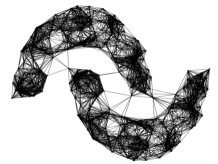
(a) RMNMF

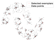
(b) SMRMF

Figure 1: Manifold approximation for 2DMoons.

Table 2: Clustering performance on 2-moons.

Evaluation	2DMoons		10DMoons
	RMNMF	SMRMF	RMNMF	SMRMF
ACC	0.8640	0.8800	0.6880	0.9240
NMI	0.4282	0.5391	0.1998	0.6521

The main contributions of our paper are as follows: (1) We propose a novel algorithm (SMRMF) to jointly learn both a sparse set of exemplars and their neighbor affinities, and data factorization, thereby allowing the exemplar selection and the data factorization to be interdependent; (2) SMRMF facilitates a data-driven selection of $k$-neighborhoods with low dispersion, and learns pairwise affinities which reflect the global structure of data, thus enabling a discriminative data representation in the latent feature space; (3) In contrast with the existing manifold regularization approaches for standard NMF, we perform exemplar selection and affinity learning in a kernel-mapped space, while factorizing the data in the input space to preserve the interpretability of NMF; (4) We develop a fast approximation of SMRMF by relaxing the constraints on the exemplar selection objective, and formulate the learning of sparse pairwise affinities as a convex optimization problem; (5) Our empirical evaluation shows that the proposed approaches are competitive against state-of-the-art manifold regularization and clustering algorithms.

2 Related Work.

In this section, we briefly discuss related work on manifold regularization and data subset selection.

Manifold Regularization. The authors of [8] were the first to introduce a graph-based manifold regularization approach for NMF, and proposed a multiplicative updating algorithm to minimize the NMF loss function. In [16], a robust formulation of NMF is proposed which uses the $L_{2,1}$ norm for the loss function, to handle noise and outliers. An augmented Lagrangian Multiplier (ALM) method is derived in [16] to optimize the regularized robust NMF loss function. The authors of [17] proposed a Laplacian-based method to simultaneously learn pairwise data similarities and a clustering of the data. In [18], a similar approach is used for adaptive learning and clustering within the NMF framework. In [19], the data is projected onto a lower-dimensional subspace; affinity learning and graph clustering are then performed in the projected subspace. The aforementioned methods use the neighborhoods of all the data, and do not incorporate any global information or selection process in learning the neighborhoods.

Semi-supervised extensions to manifold regularization [6, 20, 21] utilize label information to generate pairwise constraints to improve the discriminability of classes in a latent space. In [22], labels are used to explicitly learn a block-diagonal structure on the latent representation. In [23], the algorithm takes a set of must-link and cannot-link constraints as input, and learns an optimized graph and clustering which supports the given constraints with guarantees on the cannot-link constraint pairs to be in different clusters. Other variants of manifold regularized NMF include regularization on hyper-graphs, multi-view learning, and deep learning based methods [24, 25, 26].

SMRMF is inspired by the robust loss in [16] and the adaptive learning in [18]. However, [16] does not perform adaptive learning of the pairwise affinities of the manifold. SMRMF differs from state of the art adaptive manifold regularization (such as [18, 19]) in several ways. We perform exemplar selection and affinity learning through a kernel-mapping, thereby learning a more discriminative latent representation, while also retaining the interpretability of basis vactors in the latent space. Current algorithms learn neighborhood similarity vectors independently for each data point and the learned affinities do not incorporate information about the global structure of the data. Due to the exemplar selection constraints of SMRMF, and to the nature of our manifold approximation, the learned affinity of a data point to its neighbor also depends on the pairwise affinities between the neighbor and the rest of the data. The affinities learned by SMRMF are more informative, as their values provide an ordering of the $k$-nearest neighbors of a data point, as well as their degree of affiliation w.r.t. other representative points.

Data Subset Selection. Subset selection methods have been studied extensively in the literature. Some approaches find representatives that lie in a low dimensional embedded space (e.g., CUR [13], Rank-revealing QR [27]). Other approaches, like the algorithm introduced in this paper, optimize the pairwise dissimilarities between points to select a data subset [12, 14]. Probabilistic models, such as Determinantal Point Processes (DPP, [28]) and its variants, select a diverse subset of instances from the data, by modeling negative correlations derived from pairwise similarities. Iterative Projection and Matching (IPM, [29]), a state-of-the-art subset selection method, proposes a fast data selection approach by iteratively selecting samples that capture the maximum information of the data structure, and by projecting on the null space of the remaining data. Subset selection is also inherent to certain clustering algorithms such as $K$-medoids [30] and Affinity Propagation [31]. A state-of-the-art exemplar-based subspace clustering algorithm (ESC-FFS [32]) introduces a farthest-first search algorithm to iteratively select the least well-represented data point as an exemplar within a sparse representation framework.

3 Selective Manifold Regularization.

The manifold on which the data lies is approximated by the $k$-NN graph of the data. However, in general, the cluster assumption is not equally preserved across all $k$-neighborhoods. Our aim is to improve the factorization of the data by choosing only the $k$-neighborhoods which best preserve the cluster assumption. To this end, we sparsify the $k$-NN graph by selecting a sparse subset of data points with low dispersion among their neighbors.

Let ${\mathbf{X}}\in\mathbb{R}^{m\times n}$ denote the data matrix of $n$ points ${\mathbf{x}\in\mathbb{R}^{m}}$. A robust manifold regularized matrix factorization of ${\bf{X}}$ for data clustering was proposed in [16], and is defined as follows:

(3.1) $$\operatorname*{arg\,min}_{{\mathbf{F}},{\mathbf{G}}}||{\bf{X}}-{\bf{FG}}^{T}||_{2,1}+\lambda\mathord{\mathrm{t}}\mathord{\mathrm{r}}({\bf{G}}^{T}{\bf{LG}})$$

$$\mathord{\mathrm{s}}.\mathord{\mathrm{t}}.~{}{\bf{G}}^{T}{\bf{G}}=\bm{I},{\bf{G}}\geqslant 0$$

where $tr(.)$ denotes the trace of a matrix, ${\bf{F}}\in\mathbb{R}^{m\times c}$ denotes the latent features for each of the $c$ clusters in the data, ${\bf{G}}\in\mathbb{R}^{n\times c}$ is the cluster indicator matrix, and ${\bm{I}}$ is the identity matrix. ${\bf{L}}$ is the Laplacian matrix defined as ${\bf{L}}={\bf{Deg}}-{\bf{W}}$, where ${\bf{W}}$ is the symmetric affinity matrix of the $k$-NN graph of the data, and ${\bf{Deg}}$ is the diagonal degree matrix with ${\bf{Deg}}_{ii}=\sum_{j}{\bf{W}}_{ij}$. The $L_{2,1}-$norm is less sensitive to outliers and results in a better factorization of ${\bf{X}}$. The second term in Eq. (3.1) represents the manifold regularization, which is derived in terms of the Laplacian of an affinity matrix constructed from the $k$-NN graph of the data.

We extend the matrix factorization framework in (3.1) to learn a sparse subset of data points and their pairwise affinities, on which manifold regularization is applied. We use DS3 [14], a sparse optimization algorithm based on pairwise dissimilarities, to select exemplars from the data. Given a source set $\mathbb{X}\in\mathbb{R}^{m\times M}$ and a target set $\mathbb{Y}\in\mathbb{R}^{m\times N}$, both sampled from X, and pairwise dissimilarities $\left\{d_{ij}\right\}_{i=1,2,\dots,M}^{j=1,2,\dots,N}$ between points of $\mathbb{X}$ and $\mathbb{Y}$, we find few elements of $\mathbb{X}$ that well encode the elements in $\mathbb{Y}$. The objective function of the constrained version of DS3 is:

(3.2) $$\operatorname*{arg\,min}_{z_{ij}}\sum_{j=1}^{N}\sum_{i=1}^{M}d_{ij}z_{ij}~{}~{}~{}~{}\mathord{\mathrm{s}}.\mathord{\mathrm{t}}.$$

$$\sum_{i=1}^{M}||\mathbf{z}_{i}||_{p}\leq\tau;~{}\forall{j},~{}\sum_{i=1}^{M}z_{ij}=1;~{}\forall{i,j},~{}z_{ij}\geqslant 0$$

where $z_{ij}$ is the probability that $\mathbf{x}_{i}$ is a representative of $\mathbf{y}_{j}$; $\mathbf{z}_{i}=(z_{i1},\dots,z_{iN})$; and $\tau>0$ is a parameter which controls the exemplar size. The objective function in Eq. (3.2) denotes the total cost of encoding $\mathbb{Y}$ with exemplars from $\mathbb{X}$. The constraint on the $L_{p}$ norms of the $\mathbf{z}_{i}$s induces row sparsity to select few exemplar points. Typically, the $L_{2}$ or $L_{\infty}$ norm is used. When $L_{\infty}$ is used, $\tau$ denotes the desired number of exemplars to be selected.

We incorporate the sparse optimization of Eq. (3.2) into the matrix factorization framework of Eq. (3.1), and simultaneously minimize the objectives for matrix factorization and exemplar selection. In our case, $\mathbb{X}$ = $\mathbb{Y}$. The unified objective function is given by:

(3.3) $$\operatorname*{arg\,min}_{{\bf{Z}},{\bf{F}},{\bf{G}}}||{\bf{X}}-{\bf{FG}}^{T}||_{2,1}+\lambda\mathord{\mathrm{t}}\mathord{\mathrm{r}}({\bf{G}}^{T}{\bf{L_{Z}G}})+\beta tr({\bf{D}}^{T}{\bf{Z}})$$

$$\mathord{\mathrm{s}}.\mathord{\mathrm{t}}.~{}||{\bf{Z}}||_{1,p}\leq\tau,~{}{\bf{1}}^{T}{\bf{Z}}={\bf{1}}^{T},{\bf{Z}}\geqslant 0,{\bf{G}}^{T}{\bf{G}}={\bm{I}},{\bf{G}}\geqslant 0$$

where ${\bf D}\in\mathbb{R}^{n\times n}$ contains pairwise dissimilarities between the points of $\mathbf{X}$; ${\bf{Z}}\in\mathbb{R}_{+}^{n\times n}$ ($\mathbb{R}_{+}$ is the set of non-negative real numbers) learns the affinities between points and their representatives, and identifies the exemplars; ${\bf{L_{Z}}}$ = ${\bf Deg}_{\bf{Z}}-\frac{{\bf{Z}}+{\bf{Z}}^{T}}{2}$, where ${\bf Deg}_{\bf{Z}}$ is a diagonal matrix defined as $({\bf Deg}_{\bf{Z}})_{ii}=\sum_{j}\frac{{\bf Z}_{ji}+{\bf Z}_{ij}}{2}$.

The optimization problem in Eq. (3.3) is not convex in all three variables. Hence, we solve it using the Augmented Lagrangian method (ALM, [16]). By introducing the auxiliary variables ${\bf{X}}-{\bf{FG}}^{T}={\bf{E}}$, ${\bf{G}}={\bf{H}}$, and ${\bf{Z}}={\bf{C}}$, we re-write Eq. (3.3) as follows

(3.4) $$\operatorname*{arg\,min}_{{\bf{Z}},{\bf{C}},{\bf{F}},{\bf{G}},{\bf{E}},{\bf{H}}}||{\bf{E}}||_{2,1}+\lambda\mathord{\mathrm{t}}\mathord{\mathrm{r}}({\bf{G}}^{T}{\bf{L_{Z}H}})$$

$$+\beta\mathord{\mathrm{t}}\mathord{\mathrm{r}}({\bf{D}}^{T}{\bf{Z}})+\beta{\it I_{{\bf{C}}\in S}}$$

$$\mathord{\mathrm{s}}.\mathord{\mathrm{t}}~{}{\bf{1}}^{T}{\bf{Z}}={\bf{1}}^{T},{\bf{Z}}\geqslant 0,S=\left\{{\bf{C}}:||{\bf{C}}||_{1,p}\leq\tau\right\},$$

$${\bf{E}}={\bf{X}}-{\bf{FG}}^{T},{\bf{H}}={\bf{G}},{\bf{C}}={\bf{Z}},{\bf{G}}^{T}{\bf{G}}={\bm{I}},{\bf{H}}\geqslant 0$$

The constraint $||{\bf{Z}}||_{1,p}\leq\tau$ is represented by an indicator function on the set $S$ [33], where $I_{{\bf{C}}\in S}=0$ when ${\bf{C}}\in S$, else $I_{{\bf{C}}\in S}=\infty$.

The augmented Lagrangian for Eq. (3.4) is

(3.5) $$\operatorname*{arg\,min}_{{\bf{Z}},{\bf{F}},{\bf{G}},{\bf{E}},{\bf{H}},{\bf{C}},{\bf{\Lambda}}_{1},{\bf{\Lambda}}_{2},{\bf{\Lambda}}_{3},\mu}||{\bf{E}}||_{2,1}+\lambda\mathord{\mathrm{t}}\mathord{\mathrm{r}}({\bf{G}}^{T}{\bf{L_{Z}H}})$$

$$+\beta tr({\bf{D}}^{T}{\bf{Z}})+\beta{\it I_{{\bf{C}}\in S}}+\frac{\mu}{2}||{\bf{X}}-{\bf{FG}}^{T}-{\bf{E}}+\frac{1}{\mu}{\bf{\Lambda}}_{1}||_{F}^{2}$$

$$+\frac{\mu}{2}||{\bf{G}}-{\bf{H}}+\frac{1}{\mu}{\bf{\Lambda}}_{2}||_{F}^{2}+\frac{\mu}{2}||{\bf{Z}}-{\bf{C}}+\frac{1}{\mu}{\bf{\Lambda}}_{3}||_{F}^{2}$$

$$\mathord{\mathrm{s}}.\mathord{\mathrm{t}}.~{}{\bf{G}}^{T}{\bf{G}}={\bm{I}},{\bf{H}}\geq 0,S=\left\{{\bf{C}}:||{\bf{C}}||_{1,p}\leq\tau\right\},$$

$${\bf{1}}^{T}{\bf{Z}}={\bf{1}}^{T},{\bf{Z}}\geq 0$$

where ${\bf{\Lambda}}_{1}\in\mathbb{R}^{m\times n}$, ${\bf{\Lambda}}_{2}\in\mathbb{R}^{n\times c}$, and ${\bf{\Lambda}}_{3}\in\mathbb{R}^{n\times n}$ are matrices of Lagrangian multipliers, and $\mu$ is the penalty coefficient. We solve Eq. (3.5) with alternating updates; in each step, one variable is updated and the remaining ones are kept fixed.

Our update of ${\bf{Z}}$ differs from the standard ALM procedure in two ways: (1) In each iteration, we map the data vectors represented by the latent features onto a kernel space, and learn $\bf Z$ by computing pairwise dissimilarities in the kernel space (see Section 4); (2) In each iteration, we use a subset of exemplars, as identified by $\bf{Z}$, to compute an updated neighborhood graph and its affinity matrix. Specifically, the rows of ${\bf Z}$ (${\bf z}_{i}$s) are ranked in descending order according to their $L_{2}$ norm, and the $\tau$ representatives corresponding to the highest $L_{2}$ norms are selected as exemplars.

Let $R$ be the set of selected representatives. The updated affinity matrix $\hat{{\bf{Z}}}$ is computed as follows

(3.6) $$\hat{{\bf{Z}}} ={\bf{M}}\odot{\bf{Z}}$$

$${\bf M}_{ij} =\begin{cases}1&({\bf x}_{i}\in R)\wedge({\bf x}_{j}\in k\text{NN}({\bf x}_{i}))\\ 0&\text{\it otherwise}\end{cases}$$

where $\odot$ is the Hadamard product. The Laplacian ${\bf L}_{\bf Z}$ in Eq. (3.5) is approximated as ${\bf{L_{\hat{Z}}}}$ = ${\bf Deg}_{\hat{{\bf{Z}}}}-\frac{{\hat{{\bf{Z}}}}+{\hat{{\bf{Z}}}}^{T}}{2}$. Thus, the exemplars identified at each iteration influence the manifold regularization through the Laplacian $L_{\hat{{\bf{Z}}}}$. In turn, the pairwise dissimilarities between data vectors in the latent space influence the update of ${\bf{Z}}$, where the latent space is defined by the $c$ basis vectors of ${\bf F}$.

Algorithm 1 SMRMF

1:  input: Data ${\bf{X}}\in\mathbb{R}^{m\times n}$, rank $c$, exemplar size $\tau$, ALM parameters $\mu$, $\rho$

2:  output: factor matrices ${\bf{F}}$ and ${\bf{G}}$, encoding matrix ${\bf{Z}}$

3:  ${\bf{F}},{\bf{G}}:={\text{NNSVD}}({\bf{X}})$

4:  ${\bf{D}}$: = computeDissimilarity(${\bf{X}}$)

5:  ${\bf{Z}}:$ = A2DM2(${\bf{D}}$)

6:  repeat

7:     $\hat{{\bf{Z}}}:$ = computeAffinity(${\bf{Z}}$)

8:     ${\bf{L_{\hat{Z}}}}:$ = ${\bf Deg}_{\hat{\bf{Z}}}-\frac{\hat{{\bf{Z}}}+\hat{{\bf{Z}}}^{T}}{2}$

9:      Update ${\bf{E}}$: ${\bf{e}}_{i}=\begin{cases}(1-\frac{1}{\mu||{\bf{b}}_{i}||}){\bf{b}}_{i},&\mathord{\mathrm{if}}~{}||{\bf{b}}_{i}||\geq\frac{1}{\mu}\\ 0,&\mathord{\mathrm{otherwise}}\end{cases}$ where ${\bf b}_{i}$ is the $i^{th}$ column of ${\bf{B}}={\bf{X}}-{\bf{FG}}^{T}+\frac{1}{\mu}{\bf{\Lambda}}_{1}$

10:     Update ${\bf{F}}=({\bf{X}}-{\bf{E}}+\frac{1}{\mu}{\bf{\Lambda}}_{1}){\bf{G}}({\bf G}^{T}{\bf G})^{-1}$

11:      Update ${\bf{H}}$: ${\bf{H}}_{ij}=max({\bf{J}}_{ij},0),i=1,2,\dots,n,~{}j=1,2,\dots,c.$ where ${\bf{J}}=({\bf{G}}+\frac{1}{\mu}{\bf{\Lambda}}_{2}-\frac{\lambda}{\mu}{\bf{L_{Z}}}{\bf G})$

12:      Update ${\bf{G}}={\bf{UV}}^{T}$: where ${\bf U}$ and ${\bf V}$ are left and right singular values of ${\bf{H}}-\frac{1}{\mu}{\bf{\Lambda}}_{2}-\frac{\lambda}{\mu}{\bf{L_{Z}H}}+({\bf{X}}-{\bf{E}}+\frac{1}{\mu}{\bf{\Lambda}}_{1})^{T}{\bf{F}}$

13:     Compute $\hat{{\bf{D}}}={\bf{D}}_{K}+\frac{\lambda}{\beta}{\bf{D}}_{K}^{hg}$

14:     Update ${\bf{Z}}$ using $\hat{{\bf{D}}}$ by equation (4.12)

15:     Update ${\bf{C}}$ by equation (4.13)

16:      Update ${\bf{\Lambda}}_{1}$, ${\bf{\Lambda}}_{2}$, ${\bf{\Lambda}}_{3}$, $\mu$ ${\bf{\Lambda}}_{1}={\bf{\Lambda}}_{1}+\mu({\bf{X}}-{\bf{FG}}^{T}-{\bf{E}})$ ${\bf{\Lambda}}_{2}={\bf{\Lambda}}_{2}+\mu({\bf{G}}-{\bf{H}})$ ${\bf{\Lambda}}_{3}={\bf{\Lambda}}_{3}+\mu({\bf{Z}}-{\bf{C}})$ $\mu=\rho\mu$

17:  until convergence

4 SMRMF Optimization.

Eq. (3.5) involves several variables and can be solved by alternating minimization, where one variable at a time is updated while the others are kept fixed. The variables are updated using ALM, which is a widely used approach [16, 18, 19]. The updates for variables ${\bf E}$, ${\bf F}$, ${\bf G}$, and ${\bf H}$ in (3.5) can be derived using the standard ALM procedure (see supplementary material for the derivations). Algorithm 1 summarizes SMRMF and includes the update equations of all variables. Below we describe the steps to update ${\bf Z}$ and ${\bf C}$.

Update ${\bf{Z}}$: When optimizing with respect to ${\bf{Z}}$, Eq. (3.5) becomes

(4.7) $$\operatorname*{arg\,min}_{\bf{Z}}\lambda tr({\bf{G}}^{T}{\bf{L_{Z}}}{\bf{H}})+\beta tr({\bf{D}}^{T}{\bf{Z}})+$$

$$\frac{\mu}{2}||{\bf{Z}}-{\bf{C}}+\frac{{\bf\Lambda}_{3}}{\mu}||_{F}^{2}~{}~{}\mathord{\mathrm{s}}.\mathord{\mathrm{t}}.~{}{\bf{1}}^{T}{\bf{Z}}={\bf{1}}^{T},{\bf{Z}}\geq 0$$

In order to solve for Z, Eq. (4.7) is re-written in terms of inner products of dissimilarity matrices and Z

(4.8) $$\operatorname*{arg\,min}_{\bf{Z}}\lambda\sum_{i}\sum_{j}||{\bf g}_{i}-{\bf h}_{j}||_{2}^{2}{\bf Z}+\beta tr({\bf{D}}^{T}{\bf{Z}})+$$

$$\frac{\mu}{2}||{\bf{Z}}-{\bf{C}}+\frac{{\bf\Lambda}_{3}}{\mu}||_{F}^{2}$$

$$=\operatorname*{arg\,min}_{\bf{Z}}\beta\langle{\bf D},{\bf Z}\rangle+\lambda\langle{\bf D}^{hg},{\bf Z}\rangle+\frac{\mu}{2}||{\bf{Z}}-{\bf{C}}+\frac{{\bf\Lambda}_{3}}{\mu}||_{F}^{2}$$

$$~{}\mathord{\mathrm{s}}.\mathord{\mathrm{t}}.{\bf{1}}^{T}{\bf{Z}}={\bf{1}}^{T},{\bf{Z}}\geq 0$$

where ${\bf g}_{i},{\bf h}_{j}\in\mathbb{R}_{+}^{1\times c}$ are row vectors of $\bf{G}$ and $\bf{H}$ respectively; ${\bf D}_{ij}$ is the dissimilarity between points ${\bf x}_{i},{\bf x}_{j}$ in the original space; ${\bf D}_{ij}^{hg}$ is the dissimilarity between ${\bf g}_{i}$ and ${\bf h}_{j}$, which are the encodings of ${\bf x}_{i}$ and ${\bf x}_{j}$ in the latent space spanned by the $c$ basis vectors of ${\bf F}$.

We solve the minimization in Eq. (4.8) in a kernel space. We map the data from the original and latent spaces onto new spaces via Gaussian kernels. The corresponding kernel matrices ${\bf K}$ and ${\bf K}^{hg}$ are

(4.9) $$\vspace{-0.5em}{\bf K}_{ij}=e^{-\frac{1}{2\sigma_{i}^{2}}||{\bf{x}}_{i}-{\bf{x}}_{j}||^{2}}~{}~{}~{}{\bf K}_{ij}^{hg}=e^{-\frac{1}{2\gamma_{i}^{2}}||{\bf{g}}_{i}-{\bf{h}}_{j}||^{2}}$$

where $\sigma_{i}$ and $\gamma_{i}$ are adaptive bandwidths which are set, for each point, to the distance to the $k^{th}$ nearest neighbor. We compute new pairwise dissimilarity matrices ${\bf D}_{K}$ and ${\bf D}_{K}^{hg}$ in the respective kernel spaces as follows

(4.10) $$({\bf D}_{K})_{ij}=-\frac{({\bf K}_{ij}+{\bf K}_{ji})}{2}~{}~{}~{}({\bf{D}}_{K}^{hg})_{ij}=-\frac{({\bf K}_{ij}^{hg}+{\bf K}_{ji}^{hg})}{2}$$

We replace the dissimilarity matrices ${\bf D}$ and ${\bf D}^{hg}$ in Eq. (4.8) with ${\bf D}_{K}$ and ${\bf D}_{K}^{hg}$, and approximate the minimization problem with the following

(4.11) $$\operatorname*{arg\,min}_{{\bf Z}}\beta\langle{\bf D}_{K},{\bf Z}\rangle+\lambda\langle{\bf D}_{K}^{hg},{\bf Z}\rangle+\frac{\mu}{2}||{\bf Z}-{\bf C}+\frac{{\bf\Lambda}_{3}}{\mu}||_{F}^{2}$$

$$\mathord{\mathrm{s}}.\mathord{\mathrm{t}}.~{}{\bf 1}^{T}{\bf Z}={\bf 1}^{T},{\bf Z}\geq 0$$

The dissimilarity matrices in Eq. (4.11) are combined in a unified matrix $\hat{{\bf{D}}}_{ij}=({\bf{D}}_{K})_{ij}+\frac{\lambda}{\beta}({\bf{D}}_{K}^{hg})_{ij}$. The learning of ${\bf{Z}}$ is based on the dissimilarity values in $\hat{{\bf{D}}}$, and the minimization problem is formulated as a bounded least squares problem [14].

(4.12) $$\operatorname*{arg\,min}_{\bf{Z}}\beta\langle\hat{{\bf{D}}},{\bf{Z}}\rangle+\frac{\mu}{2}||{\bf{Z}}-{\bf{C}}+\frac{{\bf{\Lambda}}_{3}}{\mu}||_{F}^{2}$$

$$=\operatorname*{arg\,min}_{\bf{Z}}\frac{\mu}{2}||{\bf{Z}}-{\bf{C}}+\frac{{\bf{\Lambda}}_{3}}{\mu}+\frac{\beta}{\mu}\hat{{\bf{D}}}||_{F}^{2}$$

$$\mathord{\mathrm{s}}.\mathord{\mathrm{t}}.~{}{\bf{1}}^{T}{\bf{Z}}={\bf{1}}^{T},{\bf{Z}}\geqslant 0$$

SMRMF performs exemplar selection and affinity learning in a kernel space, while the factor matrices F and G are updated in input space. The computation of exemplar selection and affinity learning in a kernel space has multiple advantages: (1) kernel mapping improves class separability and yields informative dissimilarities to learn exemplars and to regularize the matrix factorization; (2) the updating of factor matrices in input space avoids the kernel pre-image problem [34]; (3) each update of the matrix ${\bf Z}$ is performed on a dissimilarity matrix transformed by an adaptive Gaussian kernel with the bandwidth of each point set equal to the distance to its $k^{th}$ nearest neighbor. This operation allows pairwise affinities of farther points to effectively go to zero, thus reducing the number of variables to be updated.

Furthermore, the nature of the learned neighborhoods in SMRMF is different from the existing adaptive manifold regularization methods (e.g. AMRMF [18]). In fact, the latter learns the pairwise affinities and $k$-neighbors for each data point independently. In contrast, we impose a row-sum constraint on ${\bf Z}$ to learn a distribution over affinities for each column of ${\bf Z}$, while the $k$-NN graph for approximating the manifold are learned from each row of ${\bf Z}$, as shown in (3.6). Therefore, the learned affinity between a data point and its neighbor depends on the distribution of pairwise affinities between the neighbor and the rest of the data. As such, the resulting manifold leads to a discriminative latent representation, as the pairwise affinities are informative of the global structure of the data.

Update ${\bf{C}}$: When optimizing with respect to ${\bf{C}}$, Eq. (3.5) becomes

(4.13) $$\vspace{-0.5em}\operatorname*{arg\,min}_{{\bf{C}}}~{}\beta{\it I}_{{\bf{C}}\in S}+\frac{\mu}{2}||{\bf{Z}}-{\bf{C}}+\frac{{\bf{\Lambda}}_{3}}{\mu}||_{F}^{2}$$

$$=\operatorname*{arg\,min}_{{\bf{C}}\in S}\frac{1}{2}||{\bf{C}}-{\bf{Z}}-\frac{{\bf{\Lambda}}_{3}}{\mu}||_{F}^{2}$$

$$\mathord{\mathrm{s}}.\mathord{\mathrm{t}}.~{}S=\left\{{\bf{C}}:||{\bf{C}}||_{1,p}\leq\tau\right\}$$

which can be solved by a projection on $S$.

The factor matrices ${\bf{F}}$ and ${\bf{G}}$ are initialized by non-negative SVD [35]. ${\bf{C}}$ is initialized to a single exemplar which has the minimum sum of pairwise distances to other points, where the entries corresponding to its row are set to one. ${\bf{Z}}$ is initialized by optimizing Eq. (3.2) using accelerated ADMM (A2DM2) [36]. A2DM2 requires each of the components in its objective function to be strongly convex. The objective function components in Eq. (3.2) are not strongly convex, hence we add the squared Frobenius norm of ${\bf{Z}}$ and ${\bf{C}}$ to Eq. (3.2) to achieve strong convexity. Hence, we use the following objective function to initialize ${\bf{Z}}$ using A2DM2:

(4.14) $$\operatorname*{arg\,min}_{{\bf{Z}},{\bf{C}}}tr({\bf{D}}^{T}{\bf{Z}})+{\it I_{{\bf{C}}\in S}}+\frac{\delta}{2}||{\bf{Z}}||_{2}^{2}+\frac{\delta}{2}||{\bf{C}}||_{2}^{2}$$

$$\mathord{\mathrm{s}}.\mathord{\mathrm{t}}.~{}{\bf{Z}}={\bf{C}},||{\bf{Z}}||_{1,p}\leq\tau,{\bf{1}}^{T}{\bf{C}}={\bf{1}}^{T},{\bf{C}}\geqslant 0$$

$$S=\left\{{\bf{C}}:||{\bf{C}}||_{1,p}\leq\tau\right\}$$

where $\delta$ is set to a very small value. The Augmented Lagrangian for Eq. (4.14) is

(4.15) $$L({\bf{Z}},{\bf{C}},{\bf{\Lambda}})=\operatorname*{arg\,min}_{\bf{Z},\bf{C}}tr({\bf{D}}^{T}{\bf{Z}})+{\bf{\it I}}_{{\bf{C}}\in S}+\frac{\delta}{2}||{\bf{Z}}||_{F}^{2}$$

$$+\frac{\delta}{2}||{\bf{C}}||_{F}^{2}+\langle{\bf{\Lambda}},{\bf{Z}}-{\bf{C}}\rangle+\frac{\mu}{2}||{\bf{Z}}-{\bf{C}}||_{F}^{2}$$

$$~{}\mathord{\mathrm{s}}.\mathord{\mathrm{t}}.~{}{\bf{1}}^{T}{\bf{Z}}={\bf{1}}^{T};{\bf{Z}}\geqslant 0;S=\left\{{\bf{C}}:||{\bf{C}}||_{1,p}<=\tau\right\}$$

The pseudo code of A2DM2 applied to Eq. (4.15) is given in the supplementary material.

5 Fast Approximation of SMRMF.

Solving (3.3) is computationally expensive due to the $L_{1,p}$ norm constraint on the encoding matrix ${\bf Z}$ for exemplar selection. To speed-up the computation, we develop a fast approximation of SMRMF (f-SMRMF). We relax the constraint $||{\bf Z}||_{1,p}$ in (3.3) to a Frobenius norm $||{\bf Z}||_{F}^{2}$, and formulate a unified objective function combining the NMF loss with the relaxed exemplar selection objective. This allows the formulation of a convex optimization problem, which can be easily parallelized to solve each column of ${\bf Z}$ independently. The unified objective function of f-SMRMF is:

(5.16) $$\operatorname*{arg\,min}_{{\bf{Z}},{\bf{F}},{\bf{G}}}||{\bf{X}}-{\bf{FG}}^{T}||_{2,1}+\lambda\mathord{\mathrm{t}}\mathord{\mathrm{r}}({\bf{G}}^{T}{\bf{L_{Z}G}})+$$

$$\beta(tr({\bf{D}}^{T}{\bf{Z}})+\frac{\delta}{2}||{\bf{Z}}||_{F}^{2})$$

$$\mathord{\mathrm{s}}.\mathord{\mathrm{t}}.~{}{\bf{1}}^{T}{\bf{Z}}={\bf{1}}^{T},{\bf{Z}}\geqslant 0,{\bf{G}}^{T}{\bf{G}}={\bm{I}},{\bf{G}}\geqslant 0$$

We use the procedure in Section 4 to solve (5.16). The optimization only differs in the update of ${\bf Z}$, replacing both the updates of ${\bf Z}$ and ${\bf C}$ in Section 4. Following steps similar to (4.7)–(4.12), the update for ${\bf Z}$ becomes:

(5.17) $$\operatorname*{arg\,min}_{{\bf{Z}}}\langle\hat{{\bf{D}}},{\bf{Z}}\rangle+\frac{\delta}{2}||{\bf{Z}}||_{F}^{2}$$

$$\mathord{\mathrm{s}}.\mathord{\mathrm{t}}.~{}{\bf{1}}^{T}{\bf{Z}}={\bf{1}}^{T},{\bf{Z}}\geqslant 0$$

We exploit the fact that each column ${\bf z}_{j}$ of ${\bf Z}$ in (5.17) can be found independently, by solving the following problem for each column $\hat{{\bf d}}_{j}$ of the matrix $\hat{{\bf D}}$:

(5.18) $$\operatorname*{arg\,min}_{{{\bf z}_{j}}}~{}{\hat{\bf d}_{j}}^{T}{{\bf z}_{j}}+\frac{\delta}{2}||{{\bf z}_{j}}||_{2}^{2}$$

$$\mathord{\mathrm{s}}.\mathord{\mathrm{t}}.~{}{\bf{1}}^{T}{{\bf z}_{j}}={{\bf 1}},{{\bf z}_{j}}\geqslant 0$$

Problem (5.18) is convex and can be worked out by explicitly solving a Karush-Kuhn-Tucker (KKT) system of equations and inequalities. The time complexity of the resulting algorithm (given in the supplementary material) is $O(n^{2})$, where $n$ is the number of instances and the number of rows of ${\bf{Z}}$. Thus, the cost of computing ${\bf Z}$ in (5.17) is $O(n^{3})$. The time complexities to solve (4.12) and (4.13) are $O(n^{3})$ and $O(n^{2}\log(n)+n^{3})$, respectively. Thus, f-SMRMF replaces the two update steps for ${\bf Z}$ and ${\bf C}$ with a new single update step for ${\bf Z}$. This gives significant computational gains in the iterative optimization, as also reflected in the empirical running times reported in Section 6.

Due to the Frobenius norm relaxation on ${\bf Z}$, we need to explicitly rank and select exemplars from ${\bf Z}$ (in contrast, the $L_{1,p}$ norm constraint sets the rows of the non-exemplars to zero). We select the required number $\tau$ of exemplars from a ranking of the rows of ${\bf Z}$, ordered by their descending $L_{2}$ norms.

6 Empirical Evaluation.

We evaluate SMRMF using the data summarized in Table 3 (further details on the data are in the supplementary material). We compare our approach against several algorithms: baseline matrix factorization and manifold regularization (NMF [1], GNMF [8], RMNMF [16]), baseline subset selection (DS3 [14], DPP [28]), state of the art subset selection (IPM [29]) state of the art subspace clustering (ESC-FFS, [32]), deep matrix factorization (DSMF, [26]), and state of the art manifold regularization methods (AMRMF [18], APMF [19]). We compare two variants of SMRMF: (1) SMRMF-Euc, which learns ${\bf Z}$ in Eq. (4.8) using pairwise Euclidean distances in the input space, to assess the effect of kernel mapping; (2) SMRMF-NS, which learns ${\bf Z}$ without imposing the exemplar selection constraints.

Table 3: Summary of the data sets.

Data set	# instances	# dimensions	# classes
Wave	600	21	3
Ionosphere	351	34	2
Sonar	208	60	2
Movement	360	90	15
Musk1	476	168	2
mfeat-fac	2000	216	10
mfeat-pix	2000	240	10
Semeion	1593	256	10
ISOLET	1200	617	5
COIL-5	360	1024	5
20-news	5020	1796	20
ORL	400	4096	40
OVA_Colon	1545	10935	2

The $k$-neighborhoods of the points selected by DPP and IPM are used to selectively regularize RMNMF. The factor matrices for manifold regularization algorithms are initialized using non-negative SVD [35]. SMRMF and variants are evaluated at 10% exemplar selection. We tune the regularization parameters of the algorithms in the range $\left\{10^{-3},10^{-2},\dots,1\right\}$ and report the best results. Detailed parameter settings of the algorithms are given in the supplementary material.

6.1 Evaluation.

We evaluate the approaches using clustering accuracy (ACC), Normalized Mutual Information (NMI), and running time. Tables 4 and 5 give the clustering accuracy and NMI of the compared algorithms. NMF, GNMF, DPP, and ESC-FFS are initialized randomly; hence, their results are averaged across 30 iterations. The standard deviations of ACC and NMI of DPP are very low (of the order of 1e-15) for all the datasets, hence they are not reported. The initialization and solution of all the other methods are deterministic. DPP on 20-news and OVA_Colon could not be run to completion, and APMF could not run to completion on OVA_Colon.

Table 4: Clustering accuracy (ACC) of all methods (standard deviations are given in parentheses).

Data	NMF	DS3	GNMF	RMNMF	AMRMF	APMF	DPP	IPM	ESC-FFS	DSMF	SMRMF	SMRMF	SMRMF	f-SMRMF
											-Euc	-NS
Wave	0.55 (0.03)	0.70	0.56 (0.04)	0.71	0.78	0.63	0.71	0.74	0.53 (0.02)	0.49	0.82	0.81	0.85	0.84
Ionosphere	0.61(0.01)	0.61	0.61 (0.01)	0.64	0.65	0.69	0.64	0.66	0.56 (0.05)	0.69	0.66	0.65	0.66	0.65
Sonar	0.54 (0.004)	0.56	0.55 (1e-4)	0.56	0.60	0.60	0.56	0.58	0.53 (0.02)	0.69	0.61	0.55	0.58	0.59
Movement	0.32 (0.02)	0.34	0.32 (0.02)	0.47	0.50	0.36	0.48	0.50	0.48 (0.01)	0.35	0.52	0.48	0.51	0.52
Musk1	0.53 (1e-15)	0.54	0.53 (1e-15)	0.55	0.58	0.56	0.54	0.58	0.53 (0.01)	0.54	0.57	0.57	0.59	0.58
mfeat-fac	0.51 (0.05)	0.27	0.51 (0.05)	0.68	0.66	0.35	0.62	0.65	0.86(0.06)	0.76	0.63	0.60	0.68	0.71
mfeat-pix	0.43 (0.05)	0.32	0.44 (0.04)	0.60	0.57	0.35	0.60	0.60	0.88 (0.05)	0.71	0.60	0.54	0.63	0.66
Semeion	0.38 (0.02)	0.34	0.39 (0.02)	0.50	0.48	0.23	0.53	0.49	0.56 (0.03)	0.48	0.47	0.42	0.50	0.53
ISOLET	0.56 (0.03)	0.33	0.57 (0.03)	0.44	0.61	0.27	0.55	0.56	0.51 (0.004)	0.51	0.64	0.49	0.61	0.65
COIL-5	0.77 (0.01)	0.33	0.77 (0.01)	0.86	0.86	0.40	0.82	0.86	0.87 (0.10)	0.58	0.86	0.84	0.90	0.86
20-news	0.26 (0.01)	0.17	0.26 (0.01)	0.27	0.17	0.06	-	0.29	0.34 (0.02)	0.09	0.24	0.29	0.24	0.27
ORL	0.40 (0.02)	0.31	0.40 (0.02)	0.63	0.67	0.18	0.60	0.64	0.48 (0.02)	0.17	0.64	0.60	0.67	0.68
OVA_Colon	0.55 (1e-4)	0.79	0.81 (1e-15)	0.87	0.88	-	-	0.92	0.77 (0.0002)	0.54	0.87	0.83	0.95	0.95
AVG	0.49	0.43	0.52	0.60	0.61	0.39	0.60	0.62	0.61	0.51	0.62	0.59	0.64	0.65

Table 5: Normalized Mutual Information (NMI) of all methods (standard deviations are given in parentheses).

Data	NMF	DS3	GNMF	RMNMF	AMRMF	APMF	DPP	IPM	ESC-FFS	DSMF	SMRMF	SMRMF	SMRMF	f-SMRMF
											-Euc	-NS
Wave	0.38 (0.007)	0.38	0.38 (0.01)	0.38	0.50	0.28	0.37	0.45	0.35 (0.01)	0.21	0.50	0.49	0.52	0.52
Ionosphere	0.02 (0.006)	0.01	0.02 (0.01)	0.06	0.01	0.14	0.16	0.14	0.02 (0.02)	0.07	0.17	0.16	0.09	0.17
Sonar	0.004 (0.001)	0.01	0.01 (1e-4)	0.01	0.04	0.06	0.01	0.02	0.004 (0.01)	0.11	0.03	0.005	0.02	0.02
Movement	0.37 (0.03)	0.41	0.37 (0.03)	0.59	0.58	0.39	0.60	0.61	0.60 (0.01)	0.41	0.58	0.60	0.59	0.58
Musk1	0.01 (1e-15)	0.02	0.01 (1e-15)	0.01	0.01	0.002	0.01	0.01	0.002 (0.001)	0.013	0.003	0.003	0.01	0.01
mfeat-fac	0.50 (0.03)	0.25	0.50 (0.04)	0.58	0.61	0.31	0.56	0.57	0.80 (0.02)	0.72	0.58	0.55	0.60	0.60
mfeat-pix	0.42 (0.04)	0.30	0.42 (0.04)	0.59	0.51	0.28	0.59	0.59	0.82 (0.02)	0.65	0.56	0.55	0.57	0.61
Semeion	0.34 (0.01)	0.29	0.34 (0.01)	0.41	0.42	0.11	0.45	0.43	0.54 (0.02)	0.42	0.40	0.29	0.42	0.44
ISOLET	0.45 (0.03)	0.10	0.45 (0.03)	0.34	0.46	0.11	0.47	0.42	0.55 (0.01)	0.57	0.49	0.39	0.46	0.50
COIL-5	0.73 (0.008)	0.32	0.73 (0.01)	0.84	0.84	0.25	0.77	0.84	0.85 (0.06)	0.66	0.84	0.81	0.88	0.84
20-news	0.25 (0.009)	0.15	0.25 (0.01)	0.26	0.12	0.01	-	0.27	0.32 (0.01)	0.04	0.24	0.29	0.23	0.27
ORL	0.61 (0.02)	0.42	0.61 (0.02)	0.77	0.80	0.32	0.76	0.77	0.69 (0.01)	0.30	0.78	0.76	0.81	0.80
OVA_Colon	0.06 (1e-4)	0.01	0.00 (0.00)	0.30	0.27	-	-	0.47	0.01 (5e-3)	0.03	0.30	0.20	0.60	0.60
AVG	0.32	0.20	0.31	0.39	0.40	0.19	0.43	0.43	0.43	0.32	0.42	0.39	0.45	0.46

Table 6: Average running times (in seconds) of all methods.

NMF	DS3	GNMF	RMNMF	AMRMF	APMF	DPP	IPM	ESC-FFS	DSMF	SMRMF	SMRMF	SMRMF	f-SMRMF
										-Euc	-NS
3.02	22.99	3.96	9.78	67.23	872.64	8.64	256.50	3.71	279.23	91.91	148.45	292.47	95.77

Both SMRMF and f-SMRMF achieve the best average ACC and NMI values, with a considerable margin of improvement on average against all competitors. This demonstrates that our approach is robust under a variety of conditions. In particular, a large improvement margin was achieved by both SMRMF and f-SMRMF on the data with the largest dimensionality (OVA_Colon). SMRMF and f-SMRMF outperform both variants SMRMF-Euc and SMRMF-NS in average ACC and NMI. This confirms that kernel mapping is effective in learning informative pairwise affinities, and that some $k$-neighborhoods can be detrimental to clustering, and our approach is effective in eliminating them.

Table 6 gives the average running time (in seconds) of the algorithms. The running times for each data set are given in the supplementary material. All experiments are run using MATLAB 2019b, on a 2.3 GHz Intel Core i5 processor with 16 GB RAM. NMF is the fastest, but results in poor clustering quality due to the lack of regularization. APMF is the most expensive. f-SMRMF effectively speeds-up SMRMF, while preserving clustering quality, thus making our approach competitive also in terms of complexity.

7 Analysis.

To investigate the effect of our selection procedure, we compare the characteristics of the selected neighborhoods against those discarded. Table 7 shows the average label mismatch of neighbor pairs within the neighborhoods of the selected (SNBH) and non-selected (NSNBH) points, for SMRMF. The third column gives the difference between the two measures. A positive difference indicates that the neighborhoods of the selected points have lower label mismatch on average than the rest of the points.We observe a positive difference for the majority of the data sets. Furthermore, Tables 4 and 5 show that SMRMF achieves a considerable improvement in performance compared to RMNMF in these data sets, thereby demonstrating the effectiveness of our data selection process.

Table 7: Characterizing the learned neighborhoods.

Data set	AVG Label	AVG Label
	Mismatch	Mismatch	(NSNBH - SNBH)
	(SNBH)	(NSNBH)
Wave	0.52	0.61	0.09
Ionosphere	0.22	0.45	0.23
Sonar	0.28	0.36	0.08
Movement	0.22	0.31	0.09
Musk1	0.08	0.17	0.09
mfeat-fac	0.24	0.24	0.00
mfeat-pix	0.07	0.08	0.01
Semeion	0.36	0.47	0.11
ISOLET	0.11	0.26	0.15
COIL-5	0.46	0.20	-0.26
20-news	0.72	0.74	0.02
ORL	0.70	0.73	0.03
OVA_Colon	0.05	0.05	0.00

As highlighted in Table 1, both % Bad NN and % Bad NBH are reduced significantly after exemplar selection, for the majority of the data sets. Few data sets (Wave, Semeion, and 20-news) show a rise in % Bad NN after exemplar selection. This is likely the reason why SMRMF does not outperform RMNMF on Semeion and 20-news. Nevertheless, SMRMF still has a significant improvement over RMNMF on Wave. A plausible explanation is that the affinities learned for the bad neighbors on Wave were not large enough to influence the NMF regularization. Another factor which affects the learned affinities is the separability of data in the latent space learned in the NMF iterations. We’ll further investigate this phenomenon in our future work. We provide further analysis on the sensitivity of exemplar and neighborhood sizes, and on the convergence of SMRMF, in the supplementary material.

8 Conclusion.

We presented a novel algorithm to simultaneously select a subset of $k$-neighborhoods and learn an affinity matrix, within an MF framework. We empirically analyzed the performance of our algorithm and showed that our approach is competitive against a variety of related methods. In the future, we’ll investigate a kernelized version of our proposed unified objective function, where the factor matrices are updated in a kernel space.

References

- [1] Daniel D. Lee and H. Sebastian Seung. Algorithms for non-negative matrix factorization. In Advances in Neural Information Processing Systems 13, pages 556–562, 2000.
- [2] Hua Wang, Feiping Nie, Heng Huang, and Chris Ding. Nonnegative matrix tri-factorization based high-order co-clustering and its fast implementation. In Proceedings of the IEEE International Conference on Data Mining, pages 774–783, USA, 2011.
- [3] Jason D. M. Rennie and Nathan Srebro. Fast maximum margin matrix factorization for collaborative prediction. In Proceedings of the International Conference on Machine Learning, volume 119, pages 713–719. ACM, 2005.
- [4] Hyunsoo Kim and Haesun Park. Sparse non-negative matrix factorizations via alternating non-negativity-constrained least squares for microarray data analysis. Bioinformatics, 23(12):1495–1502, 2007.
- [5] Weixiang Liu, Nanning Zheng, and Xi Li. Nonnegative matrix factorization for EEG signal classification. In Advances in Neural Networks - International Symposium on Neural Networks, volume 3174 of Lecture Notes in Computer Science, pages 470–475. Springer, 2004.
- [6] Hyekyoung Lee, Jiho Yoo, and Seungjin Choi. Semi-supervised nonnegative matrix factorization. IEEE Signal Process. Lett., 17(1):4–7, 2010.
- [7] Olivier Chapelle, Bernhard Schlkopf, and Alexander Zien. Semi-Supervised Learning. The MIT Press, 1st edition, 2010.
- [8] Deng Cai, Xiaofei He, Jiawei Han, and Thomas S. Huang. Graph regularized nonnegative matrix factorization for data representation. IEEE Trans. Pattern Anal. Mach. Intell., 33(8):1548–1560, 2011.
- [9] Milos Radovanovic, Alexandros Nanopoulos, and Mirjana Ivanovic. Hubs in space: Popular nearest neighbors in high-dimensional data. J. Mach. Learn. Res., 11:2487–2531, 2010.
- [10] Milos Radovanovic, Alexandros Nanopoulos, and Mirjana Ivanovic. On the existence of obstinate results in vector space models. In Proceedings of the International Conference on Research and Development in Information Retrieval, pages 186–193. ACM, 2010.
- [11] Adam Berenzweig. Anchors and hubs in audio-based music similarity. PhD thesis, Columbia University, NY, USA, 2007.
- [12] Ehsan Elhamifar, Guillermo Sapiro, and René Vidal. Finding exemplars from pairwise dissimilarities via simultaneous sparse recovery. In Advances in Neural Information Processing Systems, pages 19–27, 2012.
- [13] Michael W. Mahoney and Petros Drineas. CUR matrix decompositions for improved data analysis. Proc. Natl. Acad. Sci. U.S.A., 106(3):697–702, 2009.
- [14] Ehsan Elhamifar, Guillermo Sapiro, and S. Shankar Sastry. Dissimilarity-based sparse subset selection. IEEE Trans. Pattern Anal. Mach. Intell., 38(11):2182–2197, 2016.
- [15] D.P. Bertsekas. Nonlinear Programming. Athena Scientific, 1999.
- [16] Jin Huang, Feiping Nie, Heng Huang, and Chris H. Q. Ding. Robust manifold nonnegative matrix factorization. TKDD, 8(3):11:1–11:21, 2013.
- [17] Feiping Nie, Xiaoqian Wang, and Heng Huang. Clustering and projected clustering with adaptive neighbors. In International Conference on Knowledge Discovery and Data Mining, pages 977–986. ACM, 2014.
- [18] Lefei Zhang, Qian Zhang, Bo Du, Jane You, and Dacheng Tao. Adaptive manifold regularized matrix factorization for data clustering. In International Joint Conference on Artificial Intelligence, 2017.
- [19] Mulin Chen, Qi Wang, and Xuelong Li. Adaptive projected matrix factorization method for data clustering. Neurocomputing, 306:182–188, 2018.
- [20] Haifeng Liu, Zhaohui Wu, Xuelong Li, Deng Cai, and Thomas S. Huang. Constrained nonnegative matrix factorization for image representation. IEEE Trans. Pattern Anal. Mach. Intell., 34(7):1299–1311, 2012.
- [21] Naiyang Guan, Xuhui Huang, Long Lan, Zhigang Luo, and Xiang Zhang. Graph based semi-supervised non-negative matrix factorization for document clustering. In International Conference on Machine Learning and Applications, 2012. Volume 1, pages 404–408. IEEE.
- [22] Zechao Li, Jinhui Tang, and Xiaofei He. Robust structured nonnegative matrix factorization for image representation. IEEE Trans. Neural Networks Learn. Syst., 29(5):1947–1960, 2018.
- [23] Feiping Nie, Han Zhang, Rong Wang, and Xuelong Li. Semi-supervised clustering via pairwise constrained optimal graph. In Christian Bessiere, editor, International Joint Conference on Artificial Intelligence, IJCAI 2020, pages 3160–3166. ijcai.org, 2020.
- [24] Kun Zeng, Jun Yu, Cuihua Li, Jane You, and Taisong Jin. Image clustering by hyper-graph regularized non-negative matrix factorization. Neurocomputing, 138:209–217, 2014.
- [25] Linlin Zong, Xianchao Zhang, Long Zhao, Hong Yu, and Qianli Zhao. Multi-view clustering via multi-manifold regularized non-negative matrix factorization. Neural Networks, 88:74–89, 2017.
- [26] George Trigeorgis, Konstantinos Bousmalis, Stefanos Zafeiriou, and Björn W. Schuller. A deep semi-NMF model for learning hidden representations. In International Conference on Machine Learning, volume 32 of JMLR Workshop and Conference Proceedings, pages 1692–1700, 2014.
- [27] Tony Chan. Rank revealing qr factorizations. Linear Algebra and its Applications, 88-89:67 – 82, 1987.
- [28] Alex Kulesza and Ben Taskar. Determinantal point processes for machine learning. Foundations and Trends in Machine Learning, 5(2-3):123–286, 2012.
- [29] Alireza Zaeemzadeh, Mohsen Joneidi, Nazanin Rahnavard, and Mubarak Shah. Iterative projection and matching: Finding structure-preserving representatives and its application to computer vision. In International Conference on Computer Vision and Pattern Recognition, 5414–5423, 2019.
- [30] L. Kaufman and P.J. Rousseeuw. Clustering by Means of Medoids. Delft University of Technology : reports of the Faculty of Technical Mathematics and Informatics. Faculty of Mathematics and Informatics, 1987.
- [31] Brendan J. Frey and Delbert Dueck. Clustering by passing messages between data points. Science, 315:2007, 2007.
- [32] Chong You, Chi Li, Daniel P. Robinson, and René Vidal. A scalable exemplar-based subspace clustering algorithm for class-imbalanced data. In European Conference on Computer Vision, 2018.
- [33] Stephen P. Boyd and Lieven Vandenberghe. Convex Optimization. Cambridge University Press, 2014.
- [34] James T. Kwok and Ivor W. Tsang. The pre-image problem in kernel methods. In International Conference on Machine Learning, pages 408–415. AAAI Press, 2003.
- [35] Christos Boutsidis and Efstratios Gallopoulos. SVD based initialization: A head start for nonnegative matrix factorization. Pattern Recognition, 41(4):1350–1362, 2008.
- [36] Mojtaba Kadkhodaie, Konstantina Christakopoulou, Maziar Sanjabi, and Arindam Banerjee. Accelerated alternating direction method of multipliers. In International Conference on Knowledge Discovery and Data Mining, pages 497–506. ACM, 2015.