Numerical Convergence of Hot-Jupiter Atmospheric Flow Solutions

Abstract

We perform an extensive study of numerical convergence for hot-Jupiter atmospheric flow solutions in simulations employing a setup commonly-used in extrasolar planet studies – a resting state thermally forced to a prescribed temperature distribution on a short time-scale at high altitudes. Convergence is assessed rigorously with: i) a highly-accurate pseudospectral model which has been explicitly verified to perform well under hot-Jupiter flow conditions and ii) comparisons of the kinetic energy spectra, instantaneous (unaveraged) vorticity fields and temporal evolutions of the vorticity field from simulations which are numerically equatable. In the simulations, the (horizontal as well as vertical) resolution, dissipation operator order and viscosity coefficient are varied with identical physical and initial setups. All of the simulations are compared against a fiducial, reference simulation at high horizontal resolution and dissipation order (T682 and $\bf\nabla^{\rm 16}$, respectively) – as well as against each other. Broadly, the reference solution features a dynamic, zonally (east–west) asymmetric jet with a copious amount of small-scale vortices and gravity waves. Here we show that simulations converge to the reference simulation only at T341 resolution and with $\bf\nabla^{\rm 16}$ dissipation order. Below this resolution and order, simulations either do not converge or converge to unphysical solutions. The general convergence behaviour is independent of the vertical range of the atmosphere modelled, from $\sim\!2\!\times\!10^{-3}$ MPa to $\sim\!2\!\times\!10^{1}$ MPa. Ramifications for current extrasolar planet atmosphere modelling and observations are discussed.

1 Introduction

A fundamental goal of a numerical method, as well as of a code implementing it, is to generate a solution that approximates the true solution of the solved equation(s) and whose approximation improves as the grid spacing or the reciprocal of the truncation wavenumber tends to zero. Accordingly, in computational studies there is a long history of carefully assessing, theoretically as well as empirically, the accuracy and convergence of numerical schemes and codes (e.g. Gottlieb & Orszag, 1977; Canuto et al., 1988; Boyd, 2000; Strikwerda, 2004; Durran, 2010; Lauritzen et al., 2011). In high Reynolds number flows, such as those routinely encountered in astrophysics and atmospheric physics, the flow field does not generally remain completely smooth in time – even when initialised with a smooth field. Instead, features develop with spatial scales close to, or at, the size of the individual grid cell. Such features cannot be accurately captured by any numerical method, and the errors induced often feed back on the large scales – thus exerting a significant, deleterious influence on the overall solution. In such circumstances, there is not much recourse: one generally employs the finest grid or the highest wavenumber truncation possible, along with a well-controlled dissipation that eliminates the spurious poorly-resolved features while leaving all of the well-resolved features unimpaired. In light of this, the possibility of a code erroneously converging to a ‘solution’ that does not approximate the true solution is a perennial concern in numerical studies (see e.g. Boyd, 2000, and references therein). This is especially so in fast-developing research areas, such as extrasolar planets, wherein the flows modelled often reside in a poorly-understood region of the dynamical parameter space and pose severe computational challenges (Cho, Polichtchouk & Thrastarson, 2015; Cho et al., 2019).

At present, extrasolar planet atmospheric dynamics and general circulation modelling studies commonly employ an idealised setup to generate flow and temperature distributions starting from an initial state of rest (e.g. Showman et al., 2008, 2009; Heng, Menou & Phillipps, 2011; Bending, Lewis & Kolb, 2013; Liu & Showman, 2013; Dobbs-Dixon & Agol, 2013; Mayne et al., 2014; Polichtchouk et al., 2014; Cho, Polichtchouk & Thrastarson, 2015; Mendonça et al., 2016; Tan & Komacek, 2019). Known as the ‘Newtonian cooling approximation’ (see e.g. Salby, 1996; Cho et al., 2008), the setup consists of linearly ‘dragging’ the flow temperature to a specified temperature distribution on a specified time-scale at different pressure levels. Although highly idealised, it is a reasonable and practical first representation of the forcing in the absence of detailed information. So far, a number of studies have explored separately the effects of initial condition, numerical resolution and explicit (as well as implicit) dissipation in hot-Jupiter simulations using codes solving different equations with various resolutions, algorithms and setups (e.g. Cho et al., 2008; Dobbs-Dixon & Lin, 2008; Showman et al., 2009; Thrastarson & Cho, 2010; Heng, Menou & Phillipps, 2011; Thrastarson & Cho, 2011; Polichtchouk & Cho, 2012; Bending, Lewis & Kolb, 2013; Liu & Showman, 2013; Dobbs-Dixon & Agol, 2013; Polichtchouk et al., 2014; Mayne et al., 2014; Cho, Polichtchouk & Thrastarson, 2015; Mendonça et al., 2018; Menou, 2020) However, the issue of convergence under a controlled setting with a rigorously-tested and numerically-accurate code at high resolution is still lacking. That is, a clear and robust interpretation of the simulation results, along with the true solution of the most basic setup, is yet to be realised.

In this paper, we directly address this issue. Here we report on the results from a large number (over 300) of carefully prepared pseudospectral simulations using the BOB code (Rivier, Loft & Polvani, 2002; Scott et al., 2004; Polichtchouk & Cho, 2012), with equatable simulations compared in several different ways. While the discussion is focused on hot-Jupiters and primitive equations, we emphasize that the findings here are also relevant to other tidally-synchronized objects (e.g. cool stars and telluric planets) as well as the full Navier–Stokes equations; the latter have also been used in extrasolar planet studies (e.g. Dobbs-Dixon & Lin, 2008; Mayne et al., 2014; Mendonça et al., 2016). Note that the primary difference between the primitive equations and the Navier–Stokes equations is the assumption of hydrostatic balance in the former equations. Formally, the hydrostatic assumption limits the validity of the primitive equations to flow structures with a small aspect (vertical to horizontal) ratio. The assumption also suggests a corresponding requirement for the ratio of vertical to horizontal resolutions in numerical simulations; that is, if the pressure scale height ${\cal H}$ is used as the vertical length scale, it effectively sets ${\cal L}\ga 10{\cal H}$, where ${\cal L}$ is the horizontal length scale. For hot-Jupiters, this means roughly ${\cal L}\ga R_{p}/50$, where $R_{p}$ is the planetary radius. Hence, a spatial scale range of roughly three orders of magnitude is covered by the primitive equations.

2 Methodology

We solve the traditional primitive equations (see e.g. Salby, 1996). In $\textbf{{x}}=(\lambda,\phi,p)$ coordinates representing (longitude, latitude, pressure), the equations read:

$$\frac{{\rm D}\textbf{{v}}}{{\rm D}t}\ = -\nabla_{p}\Phi-\Big{(}\frac{u}{R_{p}}\tan\phi+f\Big{)}\textbf{{k}}\times\textbf{{v}}+{\cal D}_{\textbf{{v}}}$$ (1a)

$$\frac{{\partial}\Phi}{{\partial}p}\ = -\frac{1}{\rho}$$ (1b)

$$\frac{{\partial}\omega}{{\partial}p}\ = -\nabla_{p}\cdot\textbf{{v}}$$ (1c)

$$\frac{{\rm D}T}{{\rm D}t} = \frac{\omega}{\rho\,c_{p}}+\frac{\dot{q}_{\rm{net}}}{c_{p}}+{\cal D}_{T}\,,$$ (1d)

where ${\rm D}/{\rm D}t\equiv{\partial}/{\partial}t+\textbf{{v}}\!\cdot\!\nabla_{p}+\omega{\partial}/{\partial}p$ is the material derivative; $t$ is the time; $\textbf{{v}}=(u,v)$ is the (eastward, northward) velocity (in a frame rotating with rotation rate $\varOmega$) on a constant $p$-surface; $\omega\equiv{\rm D}p/{\rm D}t$ is the ‘vertical’ pressure velocity in the rotating frame; $R_{p}$, the planetary radius, is fiducially set to be at $p\!=\!0.1$ MPa $(=1$ bar); k is the unit vector in the local vertical direction; $\nabla_{p}$ is the horizontal gradient on a constant $p$-surface; $\Phi(\textbf{{x}},t)=gz(\textbf{{x}},t)$ is the geopotential, where $g$ is the constant ‘surface gravity’ at $z=R_{p}$ with $z$ the vertical distance above $R_{p}$; $f(\phi)=2\varOmega\sin\phi$ is the Coriolis parameter, the projection of the planetary vorticity vector $2\bm{\mathit{\Omega}}$ onto k; the direction of $\bm{\mathit{\Omega}}$ orients ‘north’; $T(\textbf{{x}},t)$ is the temperature; $\cal{D}\!_{\chi}$, for $\chi\in\{\textbf{{v}},T\}$, are dissipations given by

$${\cal D}\!_{\chi}\ =\ \nu_{2\mathfrak{p}}\big{[}(-1)^{\mathfrak{p}+1}\nabla\!_{p}^{\,2\mathfrak{p}}+{\cal C}\big{]}\,\chi\,,$$ (2)

where $\nu_{2\mathfrak{p}}$ is the constant dissipation coefficient; $\mathfrak{p}\in\mathbb{Z}^{+}$ is the order of the dissipation (not to be confused with the pressure $p$); ${\cal C}=(2/R_{p}^{2})^{\mathfrak{p}}$ is a term that compensates the damping of uniform rotation by $\cal{D}\!_{\textbf{{v}}}$, thus preserving angular momentum conservation (see e.g. Polichtchouk et al., 2014); $\rho(\textbf{{x}},t)$ is the density; $c_{p}$ is the constant specific heat at constant pressure; and, $\dot{q}_{\rm{\tiny net}}(\textbf{{x}},t)$ is the net diabatic heating rate. Note that the $\mathfrak{p}\!>\!1$ instantiations of ${\cal D}\!_{\chi}$ are known as ‘hyper-dissipation’ (e.g. Cho & Polvani, 1996a; Thrastarson & Cho, 2011; Polichtchouk & Cho, 2012). Broadly, hyper-dissipation has the effect of extending the inertial range by focusing the energy dissipation rate to a narrow range of wavenumbers near the truncation scale; this can be readily seen by taking the scalar product of equation (1a) with v and then spectral transforming the resulting equation.

Equations (1) are closed by the equation of state for an ideal gas, $p=\rho{\cal R}T$, where ${\cal R}$ is the specific gas constant. A useful variable is the potential temperature, $\Theta(\textbf{{x}},t)\equiv T(P_{\rm ref}/p)^{\kappa}$, where $p_{\rm ref}$ is a constant reference pressure and $\kappa\equiv{\cal R}/c_{p}$: when $\dot{q}_{\rm net}\!=\!{\cal D}_{T}=0$, $\Theta$ is materially conserved (i.e. ${\rm D}\Theta/{\rm D}t=0$). The equations are also supplemented with the ‘free-slip’ boundary condition (i.e. ${\rm D}p/{\rm D}t=0$) at the top and bottom $p$-surfaces; note that the top and bottom boundaries are material surfaces, across which no mass is transported. With these boundary conditions, the equations permit a full range of large-scale motions for a stably-stratified, un-ionized atmosphere – with the exception of sound waves: in equations (1), sound waves are filtered out from the full compressible hydrodynamics equations via the combination of the hydrostatic balance condition, described by equation (1b), and the free-slip boundary conditions at the top and bottom. However, the results presented in this study also apply to simulations solving the full Navier-Stokes (non-hydrostatic) equations employing a similar physical setup, as fast gravity waves admitted by both the hydrostatic and non-hydrostatic equations approach the speed of sound waves in the modelled atmospheres (see Table 1).

In this work, equations (1) and (2) are solved in the ‘vorticity-divergence and potential temperature’ form in the BOB code, a highly-accurate and well-tested code for extrasolar planet flow applications (Polichtchouk & Cho, 2012; Polichtchouk et al., 2014; Cho, Polichtchouk & Thrastarson, 2015). BOB is essentially a multi-layer extension of the 1-layer codes used in the high-resolution, turbulent studies of giant planets by Cho & Polvani (1996a, b) and Cho et al. (2003, 2008). The time integration of the equations in all of these codes is performed using a second-order accurate, leap-frog scheme with a small amount of Robert–Asselin filter applied to suppress the computational mode arising from the scheme (Robert, 1966; Asselin, 1972). The time-step size $\Delta t$ in all the simulations are such that the Courant-Friedrichs-Lewy (CFL) number (e.g. Strikwerda, 2004; Durran, 2010) is well below unity – typically $<0.3$.

Table 1: Physical, Numerical and Scale Parameters: ^(a) based on $c_{p}$; ^(b) for $\{{\rm H}_{2},{\rm He}\}$; ^(c) at $p=0.1$ MPa; ^(d) at $p=1$ KPa

Planetary rotation rate	$\Omega$	2.1$\times$10-5	s-1
Planetary radius	$R_{p}$	108	m
Surface gravity	$g$	10	m s-2
Specific heat at constant $p$	$c_{p}$	1.23$\times$104	J kg-1 K-1
Specific gas constant(a,b)	${\cal R}$	3.5$\times$103	J kg-1 K-1
Initial temperature(c)	$T_{m}$	1600	K
‘Equil.’ sub-stellar temp.(c)	$T_{e_{\rm d}}$	1720	K
‘Equil.’ anti-stellar temp.(c)	$T_{e_{\rm n}}$	1480	K
Thermal relax. time (d)	$\tau_{\rm th}$	$\approx\!10^{5}$	s
Pressure at top	$p_{\rm top}$	0	MPa
Pressure at bottom	$p_{\rm bot}$	$[0.1,10]$	MPa
Pressure w/o forcing	$p_{0}$	$\geq 1$	MPa
Truncation wavenumber	T	$[21,682]$
Number of levels (or layers)	L	$[3,1000]$
Max. sectoral wavenumber	$M$	$=\mbox{T}$
Max. total wavenumber	$N$	$=\mbox{T}$
Dissipation operator order	$\mathfrak{p}$	$[1,8]$
Viscosity coefficient	$\nu_{2\mathfrak{p}}$	(see text)	m2p s-1
(Hyper)dissip. wavenumber	$n_{d(2\mathfrak{p})}$	(see text)
Vertical length scale	${\cal H}$	$\sim\!{\cal R}T_{m}/g$	m
Horizontal length scale	${\cal L}$	$\!\ga R_{p}/20$	m
Maximum jet speed	${\cal U}$	$\!\ga 2\!\times\!10^{3}$	m s-1
Sound speed(c)	$c_{s}$	$\approx\!2.8\!\times\!10^{3}$	m s-1
Dissipation time-scale	$\tau_{d}$	$\sim\!2\!\times\!10^{5}$	s
Brunt-Väisälä frequency	${\cal N}$	$\sim\!2\!\times\!10^{-3}$	s-1
Rossby number	$R_{\rm o}$	$\equiv{\cal U}/(\Omega{\cal L})$
Froude number	$F_{\rm r}$	$\equiv{\cal U}/\sqrt{g{\cal H}}$
Rossby deformation scale	${\cal L}_{\cal R}$	$\equiv\sqrt{g{\cal H}}/\Omega$

For each $p$-surface, the code transforms the equations to the spectral space with a ‘triangular truncation’ – i.e. up to $N\!=\!M$ wavenumbers retained in the Legendre expansion,

$$\xi(\lambda,\mu,t)\ =\ \sum^{M}_{m=-M}\sum^{N}_{n=|m|}\xi^{m}_{n}(t)\,Y^{m}_{n}(\mu,\lambda)\,.$$ (3)

Here $\xi$ is an arbitrary scalar field; $n$ and $m$ are the total and sectoral wavenumbers, respectively, with $n\in\mathbb{N}\!\equiv\!\{0,1,2,\ldots\}$ and $m\in\mathbb{Z}\!\equiv\!\{\ldots,-2,-1,0,1,2,\ldots\}$; $(N,M)=(\max\{n\},\max\{m\})$; $Y^{m}_{n}(\lambda,\mu)\equiv P^{m}_{n}(\mu)\,e^{im\lambda}$ are the spherical harmonic functions, where $\mu\!\equiv\!\sin\phi$ and $P^{m}_{n}$ are the associated Legendre functions; and, $\xi^{m}_{n}(t)$ are the Legendre coefficients. The set $\{Y^{m}_{n}\}$ are the eigenfunctions of the Laplacian operator in spherical coordinates:

$$\nabla^{2}\,Y^{m}_{n}\ =\ -\!\left[\frac{n(n+1)}{R_{p}^{\ 2}}\right]Y^{m}_{n}\,,$$ (4)

where

$$\nabla^{2}\ =\ \frac{1}{R_{p}^{\ 2}}\left\{\frac{{\partial}}{{\partial}\mu}\left[\left(1-\mu^{2}\right)\frac{{\partial}}{{\partial}\mu}\right]\,+\,\frac{1}{1-\mu^{2}}\frac{{\partial}^{2}}{{\partial}\lambda^{2}}\right\}\,.$$ (5)

The $\{Y^{m}_{n}\}$ constitutes a complete, orthogonal expansion basis (e.g. Byron & Fuller, 1992). Note that, modulo ${\cal C}$, equation (2) reduces to the Laplacian operator acting on $\chi$ when $\mathfrak{p}=1$. Note also that a representation in spectral space with a truncation wavenumber T (not to be confused with the temperature $T$, and equalling $N\!=\!M$ in triangular truncations) is transformed to a Gaussian grid in physical space with approximately $(3\mbox{T},3\mbox{T}/2)$ points in the $(\lambda,\phi)$-direction: a table of grid sizes for different T numbers are provided for the reader’s convenience (Table 2). However, the Gaussian grid should not be directly compared with the grid of a finite-difference (or other grid-based) methods, as the Gaussian grid is effectively equivalent to a much higher resolution than a finite-difference grid with the same number of points as the former grid. This is due to the pseudospectral method’s accuracy and convergence properties: a smooth field is accurately represented by 2 to 3 points on the Gaussian grid, whereas 6 to 10 points are nominally needed on a finite-difference grid (e.g. Boyd, 2000; Durran, 2010). The use of $\mathfrak{p}\gg 1$ dissipation order in spectral methods also results in a comparatively much higher effective resolution, due to the narrower range of dissipated wavenumbers (e.g. Cho & Polvani, 1996a).

Vertically, the domain is decomposed into $\mbox{L}\in\mathbb{Z}^{+}$ uniformly-spaced points (or layers) in the $p$-coordinate. Along this direction, a second-order finite-difference scheme is used – as is common in codes solving equations (1) (e.g. Durran, 2010). Given the range, $p\in[p_{\rm top},p_{\rm bot}]$, the dynamically active levels $p_{k}$ for $k\in[1,\mbox{L}]$ are located at

$$p_{k}\ =\ \Big{(}k-\frac{1}{2}\Big{)}\Big{[}\frac{p_{\rm bot}-p_{\rm top}}{\mbox{ L}}\Big{]}\,.$$ (6)

The $p_{\rm top}$ and $p_{\rm bot}$ surfaces are dynamically not active, but they enforce the boundary conditions. Note that many studies employ a $\log(p)$-spacing (e.g. Liu & Showman, 2013; Cho, Polichtchouk & Thrastarson, 2015). However, the difference in the vertical spacing does not alter the main conclusions presented in this paper in any qualitative way.

Table 2: Truncation wavenumber and corresponding Gaussian grid:

Truncation	Grid  (longitude $\times$ latitude)
T682	$2048\times 1024$
T341	$1024\times 512$
T170	$512\times 256$
T85	$256\times 128$
T42	$128\times 64$
T21	$64\times 32$

Explicit dissipation plays an important role in this work, as have been in essentially all atmospheric circulation and global climate simulation works (e.g. Hamilton & Ohfuchi, 2008; Lauritzen et al., 2011, and references therein). The general effects of dissipation, including hyperdissipation, on fully-developed turbulence for the $\mbox{L}=1$ case is described in detail in Cho & Polvani (1996a). As in that work, a rational procedure is used in this work to estimate the optimal value of $\nu_{2\mathfrak{p}}$. We choose $\nu_{2\mathfrak{p}}$ so as to damp oscillations near the truncation wavenumber T on an $e$-folding time scale $\tau_{d}$ :

$$\nu_{2\mathfrak{p}}\ \approx\ \frac{1}{\tau_{d}}\left[\frac{R_{p}^{\ 2}}{\mbox{T}\,(\mbox{T}+1)}\right]^{\mathfrak{p}}\,.$$ (7)

The precise value is chosen heuristically by examining the kinetic energy spectrum and physical space fields over time, in a series of carefully-prepared simulations. It is important to note that, while the procedure is generically applicable, the precise parameter value and, more broadly, general solution characteristics (such as ‘the critical resolution for convergence’) is problem as well as setup specific. Given the above-mentioned association with the poorly-understood region of the parameter space, a separate convergence test for each problem and setup is strongly advised, particularly for extrasolar planet flow studies – as seen below and noted in Thrastarson & Cho (2011), Polichtchouk et al. (2014), and Cho, Polichtchouk & Thrastarson (2015).

The primary goal of the present study is to assess rigorously the numerical convergence of current extrasolar planet atmospheric flow simulations with a setup that is commonly-employed (e.g. Liu & Showman, 2013; Cho, Polichtchouk & Thrastarson, 2015). The chosen setup is for a model hot-Jupiter, HD209458b (Table 1). As in many studies, the thermal forcing – the $\dot{q}_{\rm{\tiny net}}/c_{p}$ term in equation (1d) – is crudely represented by a simple, linear relaxation on a timescale of $\tau_{\rm th}(p)$ to a specified ‘equilibrium’ temperature distribution $T_{e}(\lambda,\phi,p)$; note that here both $\tau_{\rm th}$ and $T_{e}$ are independent of the flow. Details of the $\tau_{\rm th}$ and $T_{e}$, as well as the initial $T$ are given in Liu & Showman (2013) and Cho, Polichtchouk & Thrastarson (2015). Note also that, unlike in Liu & Showman (2013), a strong Rayleigh dissipation in equation (1a) is not applied near the bottom of the domain in the present work. As reported by Cho, Polichtchouk & Thrastarson (2015), such a dissipation coerces the flow to a dynamically simple state – one essentially devoid of vortices and waves. This is very different than the states reached by all the simulations in this paper. Because such dissipation is physically arguable for giant planets and because employing additional dissipation or energy-conserving schemes (as a strategy to preserve stability, for example) can greatly distort solutions (Boyd, 2000), we purposely avoid this expediency in order to provide a more lucid account.

From hereon, the planetary radius $R_{p}$ and rotation period $\tau$ ($\equiv~{}2\pi/\Omega=3.025\!\times\!10^{5}$ s) are used as the length and time scales, respectively – whenever clarity is not at risk. For example, $\nu_{2\mathfrak{p}}$ is in the units of $R_{p}^{2\mathfrak{p}}\,\tau^{-1}$, and $n$ is in the units of $R_{p}^{-1}$; however, the temperature $T$ and pressure $p$ remain in the units of K and MPa, respectively. Then, for all the simulations discussed in this paper, $p_{\rm top}=0$, but $p_{\rm bot}$ is either $=\!0.1$ or $>\!0.1$. If $p_{\rm bot}=0.1$, the modelled atmosphere is designated, a ‘shallow atmosphere’; else, it is designated, a ‘deep atmosphere’. In this study, solutions are compared in the spectral, physical and temporal spaces. Examinations in all three spaces are required for a robust assessment of convergence, as it can at times appear to be attained in one or even two of the spaces.

3 Results

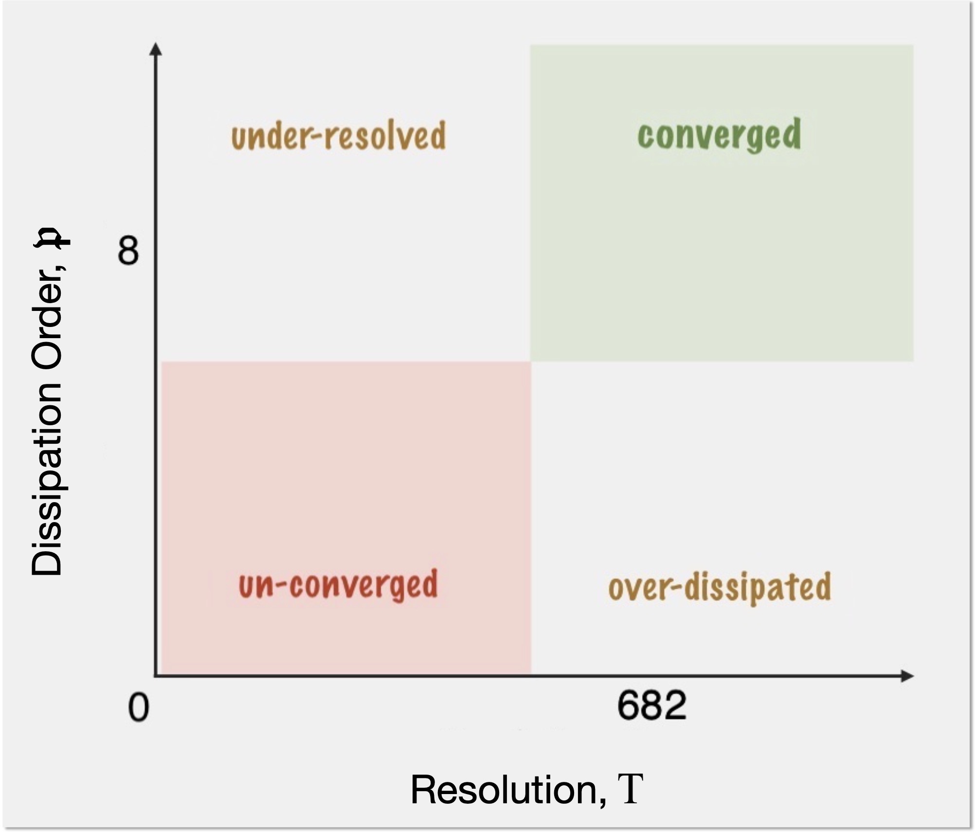
Figure 1: Summary of convergence – in dissipation order–horizontal resolution ($\mathfrak{p}$–T) space for simulations with $[0.0,0.1]$ MPa vertical domain. High T and high $\mathfrak{p}$ are required for convergence – e.g. T $\geq$ 341 and $\mathfrak{p}>6$ (green shaded area). Simulations with low T erroneously ‘converge’ to an unphysical state because they do not include interactions with small-scales. Simulations with low $\mathfrak{p}$ also erroneously ‘converge’ to an unphysical state, as energy is effectively dissipated at all scales (including the large-scales). Simulations with inadequate T and low order $\mathfrak{p}$ are not converged (red shaded area) because they are both under-resolved and over-dissipated. A high vertical resolution (e.g. L $\ga\!10$, over the $p$-range given above) – along with high T and high $\mathfrak{p}$ – is also necessary for convergence. These requirements for convergence are primarily due to the physical nature of the planet (e.g. relatively high $T_{m}$ and moderate $\Omega$, common among many short-period objects), and the simulation setup employed – in particular, high-amplitude thermal forcing with a short relaxation time, leading to a high-speed turbulent flow.

Fig. 1 summarizes the basic result of this study. It illustrates the ‘area of convergence’ in $\mathfrak{p}$–T (order–resolution) parameter space. As depicted, high T and high $\mathfrak{p}$ are both required for convergence (green shaded area). Even with a high T, simulations with a low $\mathfrak{p}$ ‘converge’ to an erroneous state, since energy is in effect dissipated at all scales – including the large-scales. With a high $\mathfrak{p}$ but a low T, simulations also ‘converge’ to an unphysical state, as they preclude small-scales from interacting (since the scales are not represented). With both low T and low $\mathfrak{p}$, simulations are not converged (red shaded area), as they are both under-resolved and over-dissipated. The lack of convergence and accuracy outside the green shaded area is principally caused by truncation and discretization errors, as well as ill-effects from ‘stability-enhancing’ strategies. We note here that most of the past extrasolar planet atmosphere simulations reside in the red shaded area (see discussions in Thrastarson & Cho, 2011; Polichtchouk & Cho, 2012; Polichtchouk et al., 2014; Cho, Polichtchouk & Thrastarson, 2015; Cho et al., 2019).

In an extended parameter space which includes the vertical resolution, nominally $\mbox{L}\approx 10$ (over the $p\in[0.0,0.1]$ range) is also necessary for convergence – along with the high T and high $\mathfrak{p}$ already discussed. For larger $p$-range, larger L is necessary. This is related to the amplitude and type of forcing applied (prescribed with $\max\{|\nabla\!_{p}T|\}\approx 10^{3}$ K on an extremely short relaxation time $\tau_{\rm th}$) – and, crucially, the complex turbulent flow resulting from it. The generated flow contains large-scale meandering high-speed jets and large-scale vortices (generally in pairs), along with many energetic small-scale vortices and waves that strongly influence the large-scale flow. Note that a physically more sophisticated forcing, based on coupling with a one-dimensional radiative transfer model (e.g. Showman et al., 2009), does not mitigate the L requirement – as well as the T and $\mathfrak{p}$ requirements – because similar flows are still generated. As emphasized in Cho, Polichtchouk & Thrastarson (2015), the ageostrophic nature of the modelled atmosphere (i.e. Rossby number $R_{\rm o}$ and Froude number $F_{\rm r}$ both of order unity) and the forcing and initialization setup commonly used all work in concert to impose an uncommonly stringent requirement on numerical codes.

In what follows, we first present the results from a very high resolution simulation – as a fiducial reference solution. Then, we discuss the convergence behaviour with respect to the horizontal resolution T, dissipation order $\mathfrak{p}$ and coefficient $\nu_{2\mathfrak{p}}$ and vertical domain range (shallow/deep atmosphere) and resolution L. Always equatable solutions within a set of simulations are compared, with each other (as well as with the reference solution). Here ‘equatable’ refers to that quality shared by simulations for which the value of a single parameter is different while those for all others are identical – possibly with the exception of a parameter or two that must be adjusted concomitantly to maintain constancy of certain ‘global’ property (e.g. $\Delta t$ for the CFL number). The procedure for adjusting $\nu_{2\mathfrak{p}}$ with varying T or $\mathfrak{p}$, described in section 2 and used in virtually all the simulations discussed in this paper, is another example of rendering simulations equatable – i.e. as $\mathfrak{p}$ is varied, $\nu_{2\mathfrak{p}}$ is changed to maintain the same dissipation rate at the truncation wavenumber, $n=\mbox{T}$. Through the equatable comparisons, we find that the $\{\mbox{T},\mathfrak{p},\mbox{L}\}$ requirement for convergence is robust up to the highest horizontal resolution investigated in this study (T682), and it is expected to hold at higher resolutions valid for equations (1).

3.1 Reference Solution

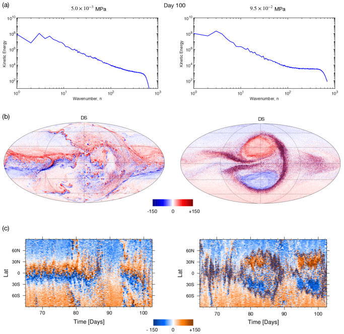
Figure 2: The reference solution – from a T682L20 simulation at $p$-levels, $5.0\times 10^{-3}$ (left column) and $9.5\times 10^{-2}$ (right column), (in units of MPa): (a) kinetic energy spectra at $t=100$ (in units of the planetary rotation period $\tau$); (b) relative vorticity fields (in units of $\tau^{-1}$) in Mollweide projection centred on the sub-stellar point; (c) $\phi$–$t$ Hovmöller plots of the relative vorticity at the longitude, $\lambda\!=\!0$, for $t\in[65,102.5]$ duration. The dissipation order is $\mathfrak{p}\!=\!8$, viscosity coefficient $\nu_{16}=2.3\!\times\!10^{-48}$ (in units of $R_{p}^{16}\,\tau^{-1}$, where $R_{p}$ is the planetary radius) and time-step size is $\Delta t=2\!\times\!10^{-5}$ (in units of $\tau$). After an initial build-up period, the spectra at all $p$-levels are broad and show a shallow sub-spectra for wavenumbers (in units of $R_{p}^{-1}$), $n\ga 100$ (particularly noticeable at $p\ga 10^{-2}$) (a), reflecting the flows (b). At $p=5.0\times 10^{-3}$, a high-speed, zonally-asymmetric equatorial jet is unstable and generates a large number of medium- and small-scale, long-lived vortices (b, left); the fast eastward jet is periodically countered by a slower eastward jet – leading to the former’s disruption, for example, at $t\approx 86$ (c, left). At $9.5\times 10^{-2}$, the flow is dominated by two modons straddling the equator, a cyclonic pair (demarcated by a high-speed, sharp front surrounded by a large number of small-scale vortices) and a much weaker, diffused anticyclonic pair covering a significant portion of the remaining space (b, right); the cyclonic modon undergoes periodic life-cycles (c, right).

In Fig. 2, we present the reference solution, which is at T682L20 resolution with $\mathfrak{p}\!=\!8$ hyper-viscosity (i.e. $\bf\nabla^{\rm 16}$ dissipation operator). As listed in Table 2, the size of the dealiasing, Gaussian grid in physical space used here is $2048\!\times\!1024$ points (see e.g. Cho & Polvani, 1996a; Boyd, 2000; Thrastarson & Cho, 2011, and references therein for discussions of dealiasing and Gaussian grid). The (non-dimensionalized) hyperdissipation coefficient and time-step size are $\nu_{16}=2.3\!\times\!10^{-48}$ and $\Delta t=2\!\times\!10^{-5}$, respectively. The vertical range of the simulation domain is $p\in[0.0,0.1]$ (in units of MPa) – i.e. of a shallow atmosphere. The figure illustrates the three types of diagnostics used to assess convergence, as discussed in section 2: the kinetic energy spectra, instantaneous flow fields and temporal evolution of the flow fields. Each diagnostic is applied to the levels near the top (left column) and bottom (right column) of the domain.

Fig. 2a shows the kinetic energy spectrum $\hat{\cal E}(n)$ of the flow field on day, $t\!=\!100$, of the simulation at the indicated $p$-levels. Here $\hat{\cal E}(n)$ is an average along the $m$-direction in spectral space for each wavenumber $n$. The figure illustrates several generic features of $\hat{\cal E}$, present at all $p$-levels in a shallow atmosphere: 1) $\hat{\cal E}$ is broad, due to the fact that a large fraction of high wavenumbers contain a significant amount of energy; 2) much more energy is contained in the low wavenumbers than in the high wavenumbers, consistent with the strong stratification of the modelled atmosphere (signified by ${\cal N}^{2}/\Omega^{2}\gg 1$, where ${\cal N}$ is the Brunt-Väisälä frequency); and, 3) a very shallow sub-spectrum (for $n\ga 100$) exists – particularly noticeable at most of the $p$-levels other than at a narrow range of levels near the top (cf. right and left panels). In contrast, the sub-spectrum for low wavenumbers possesses a much steeper slope. Feature 3) is a consequence of the ageostrophy of the modelled atmosphere: in ageostrophic atmospheres, small-scale vortices and gravity waves (‘eddies’) are readily generated and persist over long time. Here all of the above features already clearly demonstrate the need for high resolution (much higher than currently typical) in extrasolar planet atmospheric flow simulations.

Fig. 2b shows the flow fields from which the corresponding spectra in Fig. 2a have been obtained. In Fig. 2b, the instantaneous relative vorticity field $\zeta(\lambda,\phi)$ (in the units of $\tau^{-1}$) is shown in Mollweide projection, centred on the sub-stellar point: $(\lambda,\phi)\!=\!(0,0)$. Note that the modelled planet is assumed to be in a 1:1 spin–orbit synchronized state. Here $\zeta>0$ (red) in the northern hemisphere and $\zeta<0$ (blue) in the southern hemisphere indicate local rotation in the same sense as $\bm{\mathit{\Omega}}$ – and vice versa. All flow fields in this paper are shown in the same projection, and centred at the sub-stellar point, so that the entire flow field can be seen and compared easily with these fields (as well as with each other). In general, the flow near the top (left) is distinct from the flow in the rest of the domain (e.g. right), consistent with the spectral behaviour (Fig. 2a). Overall, the flow is strongly barotropic (vertically aligned) and only weakly baroclinic (vertically slanted) because of the flow near the top – as reported by Thrastarson & Cho (2010), in an earlier study using a different code. Broadly, the flow field at all $p$-levels is characterized by an undulating equatorial jet and curved, planetary-scale fronts in the northern and southern hemispheres.

More specifically, the equatorial flows in Fig. 2b are flanked by two planetary-scale modons – a pair of cyclonic vortices on the day side and a pair of anticyclonic vortices on the night side. The modons begin to form at the start of the simulation, with their centroids at the equator a distance (in units of $R_{p}$) of $\sim\!\pi$ apart in longitude at ‘full maturity’. As early as $t\approx 2$, they start to lose their north–south symmetry, showing differentiation in the $\max\{|\zeta|\}$ as well as the areal extent (despite the north–south symmetry of the prescribed forcing). This occurs because modons are not formal solutions to equations (1), with or without the forcing, and they radiate Rossby and gravity waves – even in the quasi-geostrophic regime at the beginning of the simulation (when the flow speed is low). Also apparent is the symmetry breaking between the two modons: the cyclonic modon is much stronger than the anticyclonic modon; this east–west symmetry is broken from the start of the simulation as the forcing drives westward propagating Rossby waves. The intense cyclonic modon (right) emits large-amplitude gravity waves and induce thousands of small-scale vortices to form at its periphery, with larger number of cyclones (as well as to trail it). These vortices preferentially strengthen the positively-signed, northern-hemisphere half of the cyclonic modon and screen the negatively-signed, southern-hemisphere half of the cyclonic modon – thus contributing to the north–south asymmetry; significantly, we note that the symmetry is broken only at (and above) T341 resolution. In contrast, its high-latitude position notwithstanding, the anticyclonic modon is barely visible at both $p$-levels because of the much more diffused interiors and the lack of bounding fronts. It is important to understand that, when converged, all of the above features are generic in all simulations employing the aforementioned setup.

Additionally, the cyclonic modon is very dynamic and executes a complex set of motions. Typically, the modon first forms just to the west of the sub-stellar point and initially moves in the westward direction. It then reverses direction and starts to move eastward, back towards the sub-stellar point. Near the sub-stellar point, it ‘pauses’ for a long period (up to $\sim$10 days). Then, it heads back in the westward direction, this time migrating past the western terminator and fully traversing the night side. Finally, the modon (often) dissipates completely near the eastern terminator. Subsequently, the entire ‘erratic’ motion – from formation to dissipation – repeats quasi-periodically over the duration of the simulation. Throughout this peregrination, a large number of small-scale vortices are generated and vigorous mixing on the planetary-scale is induced, which crucially affect the temperature as well as radiatively- and chemically-active species distributions. During the ‘eastward-migration phase’, if the modon manages to migrate past the sub-stellar point (instead of turning back) and reaches close to the eastern terminator, the constituent cyclones spread apart and sometimes even decouple, dissolving the modon. The overall motion described above is in sharp contrast to the essentially steady, simple westward translation observed in low-resolution simulations with low $\mathfrak{p}$, as will be seen in the ensuing sections. The complex motion is due to the nonlinear interactions with energetic small-scale eddies, not present in low T and/or low $\mathfrak{p}$ simulations.

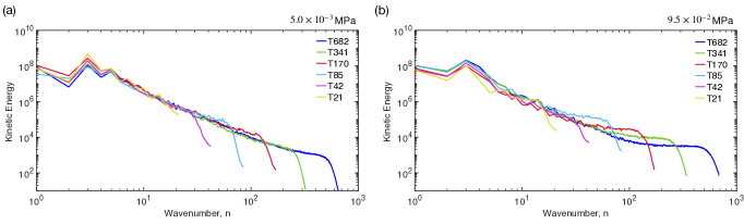
Figure 3: Kinetic energy spectra at $t=100$ from simulations which are identical to the simulation in Fig. 2 – except the horizontal resolution T, viscosity coefficient $\nu_{16}$, and the time-step size $\Delta t$. The vertical resolution of all the simulations presented is the same ($\mbox{L}\!=\!20$); but, because T varies, $\Delta t$ is halved for each doubling of the resolution – to ensure a uniform CFL condition (Boyd, 2000), given a fixed maximum flow speed. The $\mathfrak{p}\!=\!8$ dissipation operator is used in all the simulations shown: for $(\mbox{T}21,\mbox{T}42,\mbox{T}85,\mbox{T}170,\mbox{T}341,\mbox{T}682)$ resolutions, $\nu_{16}$ values are correspondingly $(2.7\times 10^{-24},4.2\times 10^{-29},6.4\times 10^{-34},9.8\times 10^{-39},1.5\times 10^{-43},2.3\times 10^{-48})$. The $p$-levels in (a) and (b) are as in figure 2; and, the T682 spectra in (a) and (b) are reproduced from figure 2a. This figure shows that simulations are definitely not converged below the T341 resolution. Spectrally, convergence “appears” to be achieved at $p=5.0\times 10^{-3}$ with T341 resolution, at least up to $n\la 200$; however, the T341 and T682 simulations still behave somewhat differently in physical space – as is suggested by the differences in the spectra for $n\ga 40$ at $p=9.5\times 10^{-2}$ (b). Full (i.e. spectral, physical, and temporal) convergence in the qualitative sense is achieved only at T341 resolution and only at the top of the atmosphere, for the physical setup employed. Note that T341 resolution here corresponds to roughly a minimum of $2048\!\times\!1024$ finite-difference grid resolution.

The complex time-dependent behaviour can be discerned in Fig. 2c, which shows the $\phi$–$t$ Hovmöller plots of the $\zeta$ field at $\lambda=0$ for the duration $t\in[65,102.5]$. The duration includes the time of the Figs. 2a and 2b. The plots in Fig. 2c illustrate the main features of the ‘flow evolution’ of a shallow atmosphere simulation at high resolution. Near the top of the domain (left), a high-speed eastward jet is obstructed by a much slower eastward jet at the equator, leading to the former’s disruption just east of the sub-stellar point at $t\approx 86$: concurrently, planetary-scale curved fronts break and roll up into vortices (Fig. 2b, left). The large variance of $\zeta$ in the $\phi$-direction is the signature of the congestion and breaking, clearly identifiable in the plot; and, it is paradigmatic of numerous such episodes occurring throughout the entire duration of the simulation (e.g. $t\in\{78,80,94\}$). Near the bottom of the domain (right), the cyclonic modon’s dominance (Fig. 2b, right) in the evolution can be seen clearly – including the signature of the aforementioned quasi-periodic life-cycles. For example, the following ‘phases’ of the cycle are detected in the plot on the right: the modon moving westward ($72\la t\la 76$), reversing direction and pausing near the sub-stellar point ($77\la t\la 86$), migrating westward all the way around the night side ($87\la t\la 94$), dissipating completely near the western terminator ($t\approx 94$) and returning to a quasi-stationary state after forming again just to the west of the sub-stellar point ($94\la t\la 101$).

3.2 Numerical Resolution

In Fig. 3, we present the kinetic energy spectrum $\hat{\cal E}(n)$, taken from simulations which are identical to the simulation of Fig. 2 in all respects – except for T (and the correspondingly adjusted $\Delta t$ and $\nu_{16}$). As discussed above, $\Delta t$ is halved for each doubling of the T value to ensure a uniform CFL condition in all the simulations presented, given the approximately constant maximum flow speed ${\cal U}$ ($\approx\!12.25$, in the units of $R_{p}\,\tau^{-1}$) across the simulations; and, $\nu_{16}$ is adjusted so that the energy dissipation rate at a given wavenumber (e.g. $n=21$) is same in all the simulations. In general, $\hat{\cal E}$ depends on $t$ – even after reaching equilibration, as the equilibration state itself can fluctuate quasi-periodically on varying time-scales for different simulations; in addition, $\hat{\cal E}$ depends on $p$ as well, as will be seen below. In the figure, all the simulations shown have reached equilibration at all the $p$-levels by $t\!\sim\!10$; and, at the time shown ($t=100$), all the spectra are representative of the mean equilibration state. The $p$-levels shown are as in Fig. 2, and the reference spectra from Fig. 2a is reproduced in Fig. 3 for ease of comparison.

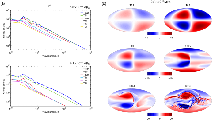
Figure 4: $\mathfrak{p}\!=\!1$ simulations identical in all respects, except the horizontal resolution (and accordingly adjusted viscosity coefficient $\nu_{2}$ and time-step size $\Delta t$): kinetic energy spectra (a) and the corresponding vorticity fields (b) at $t=82$, with $p$-levels as indicated. The $\mathfrak{p}\!=\!1$ simulations are not converged until the T341 resolution at the top and not at all below, as in the $\mathfrak{p}\!=\!8$ case (cf. Fig. 3). Significantly, the dissipation appears to affect the entire range of wavenumbers, down to the low wavenumbers – even down to $n=2$ at the T341 resolution for $p=9.5\!\times\!10^{-2}$. The relative vorticity fields below the T341 resolution exhibit meridional (north–south) symmetry (modulo the sign change due to sphericity), consistent with the dominance of viscosity seen in (a). Below the T85 resolution, the flow structures are diffused and essentially static. Above the T85 resolution, the modon exhibits dynamism that increases with resolution. Sharp, elongated fronts that roll up into small scale features emerge only at the T682 resolution; however, the flow is still distinct from the $\mathfrak{p}\!=\!8$ case (cf. Fig. 2b). The overall behavior strongly motivates the use of a higher order dissipation (preferrably $\mathfrak{p}\gg 1$; see Figs. 5 and 6).

Fig. 3 shows that simulations are definitely not converged below T341 resolution. It also shows the importance of widening the focus to more than just one $p$-level or vertical region (Cho, Polichtchouk & Thrastarson, 2015; Cho et al., 2019), as $\hat{\cal E}$ at different $p$-levels can have different convergence properties. Consider the $p=0.005$ level (Fig. 3a), for example. At first glance, convergence appears to be achieved at T42 resolution; but, spectra at the $p=0.095$ level (Fig. 3b) clearly show that convergence is actually not achieved even at T341 resolution. In Fig. 3b, spectral blocking (the raised ‘backward-facing step’ in the mid-$n$ region of $\hat{\cal E}$) is apparent in the T85, T170 and T341 spectra: such a spectral feature is produced by aliasing error in simulations which under-resolve the flow (Boyd, 2000; Thrastarson & Cho, 2011). On closer inspection, the T85 and T170 (and possibly the T42) spectra at the $p=0.005$ level also display weak spectral blocking. Typically, spectral blocking is more easily noticed occurring near $n=\mbox{T}$, particularly under quasi-geostrophic conditions, because of the steepness of $\hat{\cal E}$ (low energy content) in that region. Here high wavenumbers (i.e. $n>\mbox{T}$), energized by the flow, are aliased onto the mid-$n$ region. The feature also frequently shows up shortly before a simulation ‘blows up’. At lower resolutions, spectral blocking is altogether, or nearly so, masked by over-dissipation (T21 and T42 spectra). In this case, crucial information about physics (e.g. frontal dynamics at the modon’s periphery) is suppressed – in peril of the simulation’s verisimilitude, as shown below.

Considering spectra at both $p$-levels together, one might be tempted to argue for convergence predicated on a sub-range of wavenumbers (e.g. convergence at T85 resolution, for $n\la 20$). However, the behaviour in physical space of simulations with up to T341 resolution is still qualitatively different compared to the behaviour of simulations with T682 resolution – even at the large scales. This is not surprising, given the large difference in $\hat{\cal E}$ for $n\ga 40$ (i.e. most of the $\{n\}$ included in the simulation) and the non-linearity of equations (1). Moreover, because spectral blocking is a manifestation of accumulated errors infecting all $n$, large-scale behaviours are unreliable in simulations that evince it. Clearly, $\hat{\cal E}$ is very useful as a first diagnostic – especially at very high resolutions, when plotting one snapshot of the flow field can sometimes take more than an Earth day. In sum, convergence is achieved only at T341 resolution for the physical setup employed – and that only at the top region of the domain. Note that T341 resolution here corresponds to roughly a minimum of $2048\!\times\!1024$ finite-difference grid resolution. As far as we are aware, past simulations that use the same, or similar, setup have been performed with much lower resolutions and dissipation orders (e.g. Menou, 2020, and references therein).

At this point, the reader may wonder if high-order dissipation is necessary – or even proper. After all, the Navier–Stokes equations (from which the primitive equation derives) are with $\mathfrak{p}=1$ dissipation. We briefly address this issue here and leave the more detailed discussion for the next sub-section. Fig. 4 demonstrates clearly why the $\mathfrak{p}=1$ dissipation is not adequate (up to the resolution presented, for the setup employed). In the figure, simulations at different resolutions are presented with resolution-adjusted $\nu_{2}$ and $\Delta t$, but otherwise identical. Here $t=82$ for all the simulations. The time chosen is well after the kinetic energy time series have reached their equilibrated (i.e. quasi-stationary) states and remain qualitatively unchanged for up to 300 days. The overall behaviour in both the spectral (Fig. 4a) and physical (Fig. 4b) spaces strongly suggests the use of $\mathfrak{p}>1$ to prevent over-dissipation (in fact $\mathfrak{p}>4$, as demonstrated explicitly in the next sub-section).

Fig. 4a shows that simulations with $\mathfrak{p}=1$ are not converged, up to T341 resolution (and, in actuality, up to T682 over most of the domain). We note here that, significantly, the dissipation affects essentially the entire range of $n$ – all the way down to $n=1$ in nearly all the simulations presented (cf. Fig. 3). Fig. 4b presents the $\zeta$-fields at $p=9.5\times 10^{-2}$, from which the spectra in Fig. 4a are obtained. Here simulations with T21, T42 and T85 resolutions display meridional (north–south) symmetry – indicating the dominance of explicit dissipation, which is meridionally symmetric. Below T85 resolution, the flow structures are diffused and essentially static. At T85 and above resolutions, a moving cyclonic modon forms westward of the sub-stellar point. Crucially, the modon exhibits significant dynamism only at, and above, the T341 resolution with high $\mathfrak{p}$ (cf. Figs. 2b and 6b). These features are robust, and persist up to long integration times (e.g. here $t=300$).

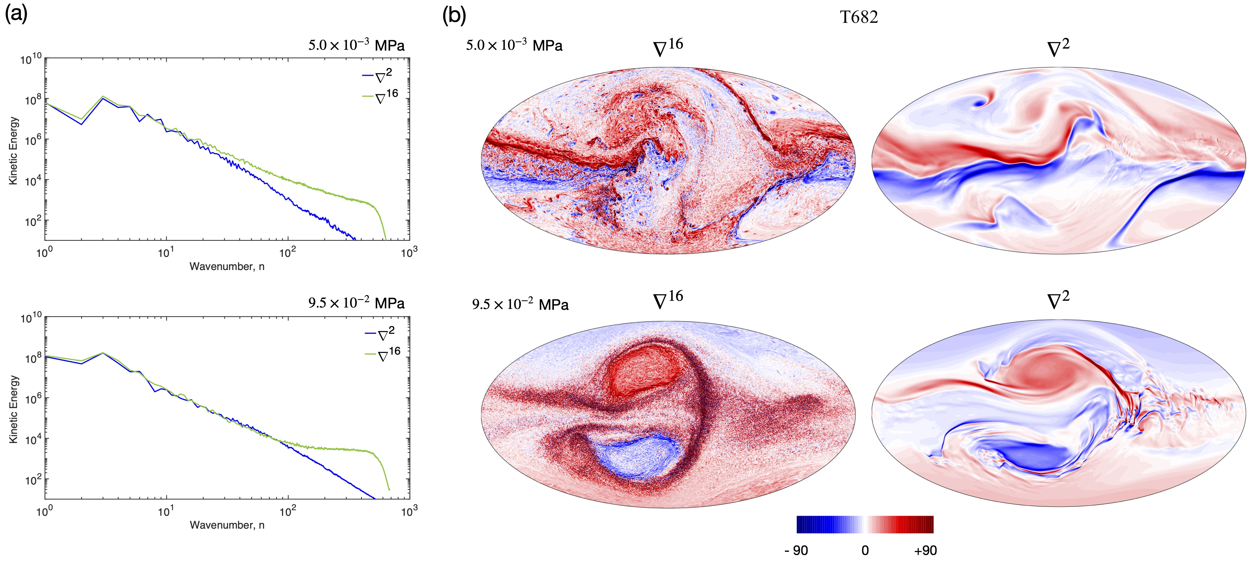
Figure 5: Two T682L20 simulations, identical in all respects except for $\mathfrak{p}\in\{1,8\}$ (and the correspondingly adjusted $\nu_{2\mathfrak{p}}$ coefficients, $\nu_{2}=1.0\!\times\!10^{-8}$ and $\nu_{16}=2.3\!\times\!10^{-48}$). The kinetic energy spectra (a) and the corresponding relative vorticity fields (b) at $t=80$. Both simulations contain similar energy contents up to $n\approx 80$ at $p=9.5\times 10^{-2}$ and only up to $n\approx 15$ at $p=5.0\times 10^{-3}$. With $\mathfrak{p}=1$, energy is excessively dissipated from high wavenumbers and the relative vorticity fields are devoid of small scale dynamics. While the energy contents of large-scales are similar in both simulations, $\mathfrak{p}=1$ simulation contains noticeably less energy at $n=2$ (at both $p$-levels). At $p=5.0\times 10^{-3}$, the $\mathfrak{p}=8$ simulation exhibits a dynamic modon, but the $\mathfrak{p}=1$ simulation does not capture the modon. At $p=9.5\times 10^{-2}$, the modon is noticeably weaker and more sluggish in the $\mathfrak{p}=1$ simulation.

The unphysical consequence of the above over-dissipation (particularly at the high $n$) is more clearly seen with T682L20 simulations, presented in Fig. 5. In the figure, two simulations with different $\mathfrak{p}\in\{1,8\}$ are presented (with accordingly adjusted $\nu_{2\mathfrak{p}}$): $(\mathfrak{p},\nu_{2\mathfrak{p}})\in\{\,(1,\,1.0\!\times\!10^{-8}),\ (8,\,2.3\!\times\!10^{-48})\,\}$; otherwise, the two simulations are identical. The kinetic energy spectra and the corresponding relative vorticity fields at $t\!=\!80$ are shown. At $p=9.5\!\times\!10^{-2}$, both simulations contain similar amounts of energy up to only $n\approx 80$ and, even more unsettlingly, only up to $n\approx 15$ at $p=5.0\!\times\!10^{-3}$. The latter is only $\sim$2% of the available range of $n$ – i.e. nearly 98% of the simulation is subjected to over-dissipation. Hence, in the $\mathfrak{p}=1$ simulation, small-scale features are suppressed in the vorticity fields (at both $p$-levels shown). Note that, while the energy content in the large-scales (e.g. $n\;\hbox to0.0pt{\lower 2.5pt\hbox{$\sim$}\hss}\raise 1.5pt\hbox{$<$}\;15$) is similar in the two simulations, the $\mathfrak{p}=1$ simulation noticeably show less energy in the $n=2$ mode (which correspond to modons) at both $p$-levels. Consequently, in the $\mathfrak{p}=1$ simulation, the modon is not present at $p=5.0\!\times\!10^{-3}$ (cyclones are detached) and is comparatively much weaker (than in the $\mathfrak{p}=8$ simulation) at $p=9.5\!\times\!10^{-2}$.

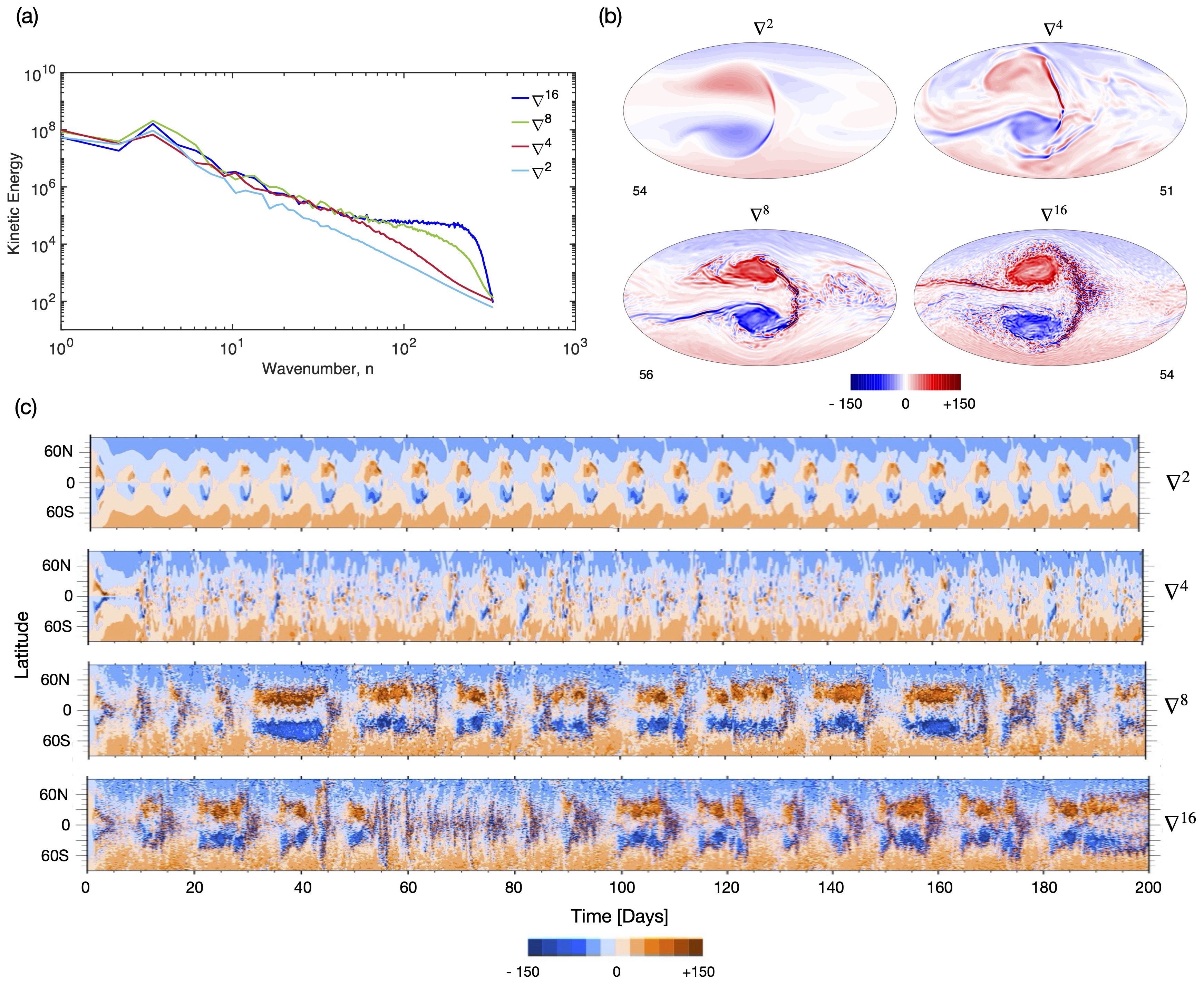
Figure 6: Kinetic energy spectra (a) of the flow fields (b) at $p=9.5\times 10^{-2}$ ($t$ is slightly different in the different frames, chosen from $[51,56]$, so that the modons are ‘in phase’) and the $\phi$–$t$ Hovmöller plots of $\zeta$ at $\lambda=0$ (c) from four T341L20 simulations – identical in setup, except for the $\mathfrak{p}$ in $\nabla^{2\mathfrak{p}}$ (and $\nu_{2\mathfrak{p}}$). For $\mathfrak{p}\in\{1,2,4,8\}$, $(\nu_{2},\nu_{4},\nu_{8},\nu_{16})=(10^{-3},10^{-8},10^{-18},10^{-43})$, so that the dissipation rate for $n=341$ is same for all $\mathfrak{p}$ and equatable comparisons can be made between the simulations. In general, lower $\mathfrak{p}$ dissipates over a broader range of $n$ as well as dissipates the higher $n$ more strongly (a). This is consistent with the more diffused, sluggish flow structures seen in the simulations (b). Note that, while these modons are associated with areas of higher temperature compared to their surroundings for all $\mathfrak{p}$ (Skinner & Cho, submitted), they should not be confused with the ‘eastward-shifted hot area’ at the lower $p$-levels (higher altitudes) in lower resolution simulations, oft discussed in the literature (see Cho et al., 2019, for more information). There is a noticeable difference in the general character of the flow with $\mathfrak{p}$. For example, note the ‘phase variation’ in the modon’s position ($t$ is given at the bottom in each frame) across the simulations. This is because modons quasi-periodically break up into small-scale storms and subsequently reform when $2\mathfrak{p}\geq 8$, while modons execute a nearly-steady translation with minor perturbation when $2\mathfrak{p}<8$. The former pair of simulations show $\sim$14 life-cycles of a modon forming on the day-side and traversing around the planet with an average period of roughly $\sim$12 $(\pm 5)$ days.

3.3 Dissipation Order

As might be expected from the previous sub-section, dissipation order $\mathfrak{p}$ strongly affects convergence. And, there exists a ‘lower bound’ on $\mathfrak{p}$ for convergence: for the setup used in this paper, $\mathfrak{p}>4$ is required (along with $\mbox{T}\geq 341$). This is shown explicitly in Fig. 6, wherein simulations at T341 resolution are presented with identical setup – except for $\mathfrak{p}$ (and, correspondingly, $\nu_{2\mathfrak{p}}$). Recall that a rational procedure is used to obtain the value of $\nu_{2\mathfrak{p}}$, resulting in the same dissipation rate at $n=\mbox{T}$ for all $\mathfrak{p}\in\{1,2,4,8\}$. This gives $(\nu_{2},\nu_{4},\nu_{8},\nu_{16})=(10^{-3},10^{-8},10^{-18},10^{-43})$: these values ensure equatable comparisons between simulations with different $\mathfrak{p}$ (e.g. Cho & Polvani, 1996a; Thrastarson & Cho, 2011; Polichtchouk & Cho, 2012). As before, convergence is diagnosed in three ways – i.e. the instantaneous $\hat{\cal E}$ at $p=0.095$ (Fig. 6a), the $\zeta$-field from which the corresponding spectrum in Fig. 6a is obtained (Fig. 6b) and the $\phi$–$t$ Hovmöller plot of the $\zeta$-field at $p=0.095$ from the simulations presented in Figs. 6a and 6b (Fig. 6c). Note that the different times of the frames in Figs. 6a and 6b (shown at the bottom of each frame in the latter) are chosen so that the modon, which forms in all the simulations in the figure, is located closest to the planet’s sub-stellar point – to adjust for the ‘phase shift’ in the modon’s position in physical space: recall that such a phase shift does not affect $\hat{\cal E}$. The plots in Fig. 6c show the differences in time, as well as in space.

In Fig. 6a, $\hat{\cal E}$ for $\mathfrak{p}\in\{1,2\}$ are dissipated much more strongly compared with that for $\mathfrak{p}\in\{3,4\}$ – particularly at high $n$. In fact, the over-dissipation is noticeable already starting at $n\approx 40$, even with $\mathfrak{p}\!=\!2$. Accordingly, Fig. 6b shows that the modons are significantly diffused and small-scale structures are also noticeably absent, when the $\mathfrak{p}\in\{1,2\}$ fields are compared with the $\mathfrak{p}\in\{4,8\}$ fields. Given this, we expect current extrasolar planet simulation studies which use $\mathfrak{p}\in\{1,2\}$ dissipation order to display a much narrower ‘energetically-significant’ spectral range and, importantly, much less dynamic large-scale flow and temperature structures. Even with $\mathfrak{p}\!=\!4$, energy content is greatly depleted for $n\ga 50$. For $\mathfrak{p}\!=\!8$, notice the dissipation range (super-exponentially decaying region at high $n$) beginning at $n=n_{d(16)}\approx 270$, signifying the presence of a proper conduit for energy and potential enstrophy effluxes at the length-scale of T; here $n_{d(2\mathfrak{p})}$ is the ‘(hyper)dissipation wavenumber’. In contrast, a dissipation range is either only weakly present or not at all present for the other $\mathfrak{p}$ values. Qualitatively, the above behaviours are generic and not restricted to a particular $p$-level or resolution (provided that the latter is at least T341).

Fig. 6b shows the non-convergence behaviour in physical space. The behaviour is again consistent with that encountered in the corresponding spectral space (Fig. 6a). In Fig. 6b, the flow field of the $\mathfrak{p}=1$ simulation is smooth almost everywhere. Both the cyclonic and anticyclonic modons that form are very diffused; and, the stronger, cyclonic modon executes a simple, quasi-steady translation in the westward direction. In the flow field of the $\mathfrak{p}=2$ simulation, the cyclonic modon’s motion is more energetic and even slightly chaotic; its two constituent cyclones can spread further apart in latitude than in the $\mathfrak{p}=1$ case, as seen in the frame. In the flow fields of the $\mathfrak{p}\in\{4,8\}$ simulations, the modon’s motion and environment are much more complex than in the $\mathfrak{p}=2$ simulation; in particular, it generates a large quantity of small-scale vortices at its periphery and in the equatorial region, primarily to its east (see also Fig. 2b, right). The principle differences between the $\mathfrak{p}\in\{4,8\}$ flow fields are more quantitative, rather than qualitative. For example, with $\mathfrak{p}=8$ the modon generates many hundreds of small-scale vortices at its periphery, compared to many tens with $\mathfrak{p}=4$. Never the less, this leads to a noticeable difference in the evolutions of $\mathfrak{p}\in\{4,8\}$ simulations, as will be seen shortly: with $\mathfrak{p}=8$ the modon is more robust and its motion is more chaotic. The general picture of these simulations is consistent with the noticeably higher energy content of the high wavenumbers in higher $\mathfrak{p}$ simulations, seen in Fig. 6a. Unsurprisingly, the general picture is also consistent with the behaviour in fully turbulent simulations reported by Cho & Polvani (1996a), due to the turbulence produced by ageostrophy here.

As just alluded to above, the non-convergence behaviour extends beyond a single time frame: it persists over a long time, as shown in Fig. 6c. In fact, it persists over the duration of the simulation, after the initial ramp-up period of $\sim$10 days. Broadly, the $\mathfrak{p}\in\{4,8\}$ simulations can be grouped apart from the $\mathfrak{p}\in\{1,2\}$ simulations according to their evolutions: the simulations in the former group evolve qualitatively similar to each other, while the simulations in the latter group evolve qualitatively different than the simulations in the former group – as well as from each other (as already discussed above). In addition to the $\mathfrak{p}=1$ flow field being essentially smooth everywhere over the entire duration, the evolution is highly periodic; this is caused by the traversal of the cyclonic modon around the planet with a period of $\approx$ 8 days. In the $\mathfrak{p}=2$ simulation, the modon is more chaotic and short lived, with its constituent cyclones ultimately detaching from each other. In contrast, in the $\mathfrak{p}\in\{4,8\}$ simulations, the modon is much more robust and its life-cycle is much more complex. That is, the cyclonic modon initially forms $\sim\!40^{\circ}$ to the west of the sub-stellar point, as in the $\mathfrak{p}\in\{1,2\}$ simulations; but, then it proceeds to oscillate back and forth between the western terminator and a point to the east of the sub-stellar point – at times ‘hanging’ on the day-side for up to $\sim\!17$ days. Throughout this phase, the modon also generates up to many hundreds small-scale vortices – later disintegrating into additional small-scale vortices and subsequently reforming (e.g. $t\approx 83$). The entire cycle repeats often. Over the duration presented in Fig. 6c, the $\mathfrak{p}\in\{4,8\}$ evolutions both exhibit $\sim$14 life-cycles of a modon forming on the day-side and traversing the planet, with an average period of $\sim$12 days (cf. period of $\approx$ 8 days in the $\mathfrak{p}\in\{1,2\}$ evolutions). The main qualitative difference between the $\mathfrak{p}\in\{4,8\}$ evolutions are the phase difference and the cycle durations.

Thus far, we have motivated the use of high-order dissipation in attaining convergence. However, we wish to underscore the point that hyperdissipation is more broadly an indispensable element in circumstances when the cost of effecting simulations with adequate resolutions is nearly prohibitive, as in extrasolar planet simulations. Consider Fig. 7, for example. It demonstrates how a low resolution simulation employing a high-order dissipation can ‘emulate’ the $\hat{\cal E}$ of a much higher resolution simulation employing a low-order viscosity – up to nearly $n_{d(2\mathfrak{p})}$ of the lower resolution simulation; recall that $n_{d(2\mathfrak{p})}$ is the fiducial dissipation scale $n_{d}$ for the given $2\mathfrak{p}$. This ability is a tremendous practical advantage. In the figure, two T42 simulations with $\mathfrak{p}=\{1,2\}$ and $(\nu_{2},\nu_{4})=(10^{-7},10^{-9})$ are compared with a T341 simulation with $\mathfrak{p}=1$ and $\nu_{2}=10^{-8}$. In the latter simulation, $\Delta t$ is reduced by 8 times to accommodate the higher T value, but all three simulations are identical otherwise. The time of all the plots in the figure is $t=75$.

In Fig. 7a, notice how increasing the dissipation order of the lower resolution simulation permits it to achieve a similar level of inviscidness – up to $n=\mbox{T}$ in this illustration (cf. green and blue full lines). In the figure, the T42 simulation with $\mathfrak{p}=1$ from Fig. 4 is reproduced for reference (black dotted line). Comparing this simulation to the T341 simulation with the same $\mathfrak{p}$ and $\nu_{2}$ (blue line), the T42 simulation is much more dissipative with the large-scale flow completely devoid of dynamism: if convergence were achieved, $\hat{\cal E}$ from the two simulations would be nearly the same up to $n\approx n_{d(2)}$ (as in the blue and green lines). We emphasize that the T42 simulation with $\mathfrak{p}=1$ here is comparable to most current extrasolar planet atmosphere flow simulations in terms of effective resolution. Unfortunately, employing high $\mathfrak{p}$ operator at T42 does not lead to convergence in extrasolar planet simulations – as discussed in section 3.2. Fig. 7b shows the flow fields from which two of the spectra in Fig. 7a (T42 with $\mathfrak{p}=2$ and T341 with $\mathfrak{p}=1$) have been obtained. The two flow fields in Fig. 7b are similar (but not identical), here again consistent with the spectra in Fig. 7a. For example, the cyclonic modon that forms west of the sub-stellar point begins to decouple when it reaches near the western terminator in both simulations. The T42 field here should be compared with the T42 field of Fig. 4, in which the modon is much weaker (N.B. the difference in scale of values) and the flow is north–south symmetric.

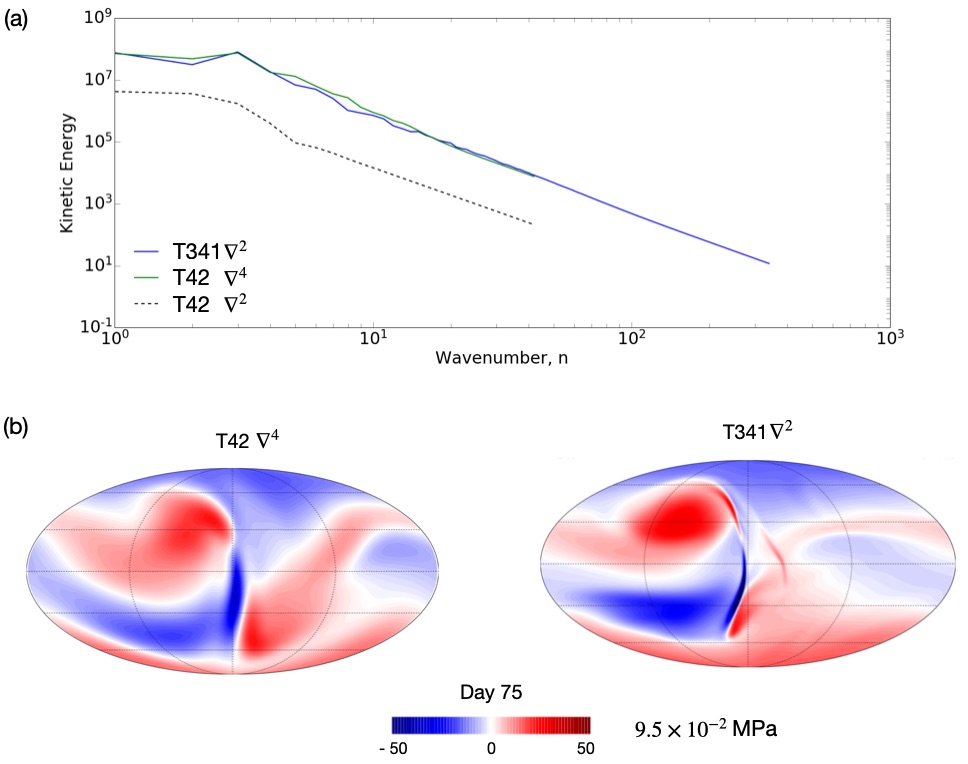
Figure 7: Kinetic energy spectra (a) and flow field (b) from simulations with $\mathfrak{p}\in\{1,2\}$ and two resolutions, T42L20 and T341L20, at $t=75$ and $p=9.5\!\times\!10^{-2}$. The T42 simulation using the higher order dissipation operator ($\mathfrak{p}=2$) permits the spectrum to be much closer to that of a T341 resolution simulation with a lower order dissipation operator ($\mathfrak{p}=1$). The flow fields in these two simulations are much more similar to each other than that from the T42 simulation using the $\mathfrak{p}=1$ operator (cf. Fig. 4b) – showing the utility of hyper-dissipation, even with lower resolution.

3.4 Deep Atmosphere

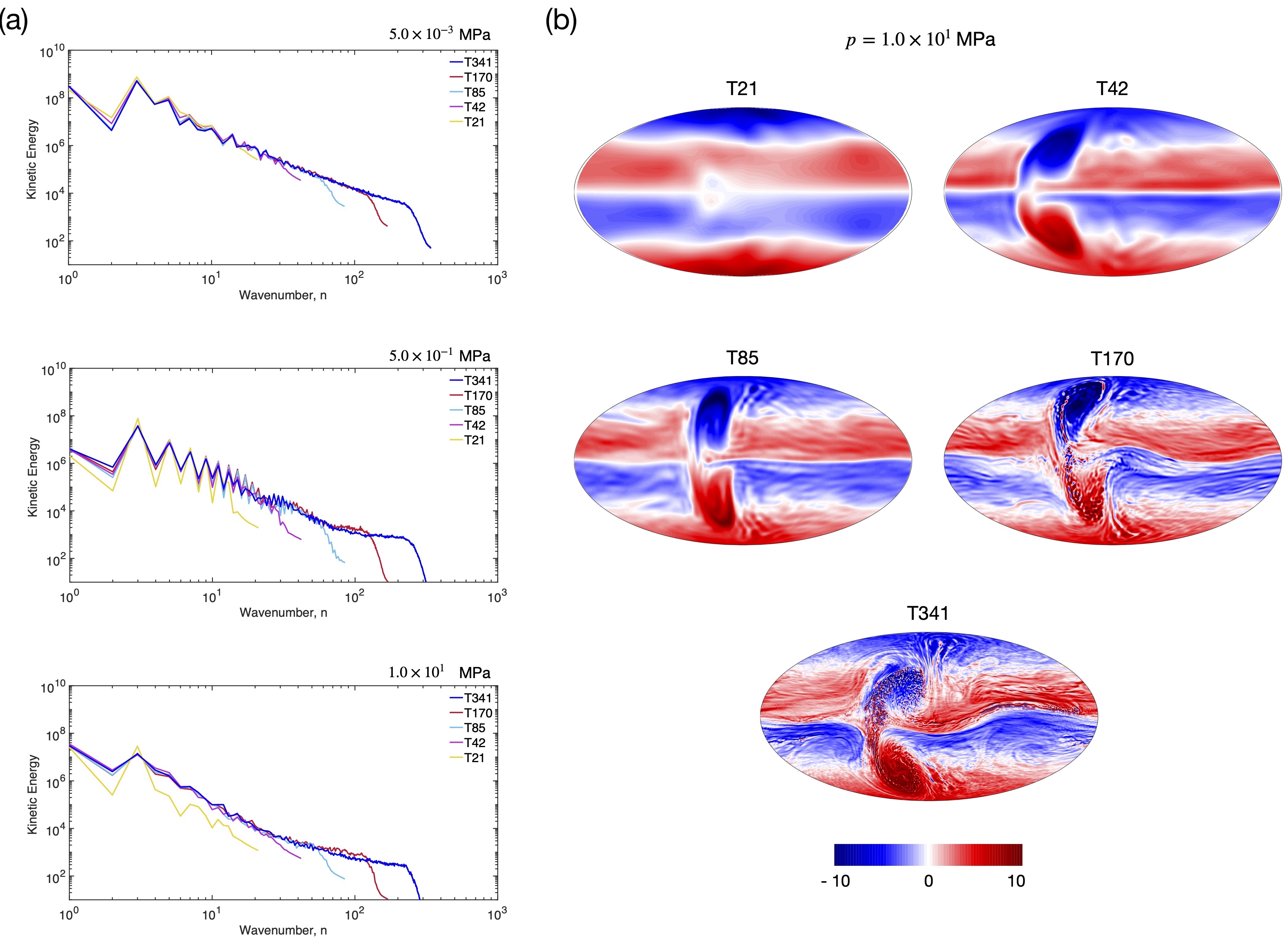
Figure 8: ‘Deep atmosphere’ simulations with vertical domain range $p\in[0,10]$ and L200 vertical resolution at different horizontal resolutions. Simulations are identical in all respects (except horizontal resolution and their correspondingly adjusted $\nu_{16}$ and $\Delta t$ values); $\mathfrak{p}=8$ in all the simulations shown. Kinetic energy spectra (a) at the $p$-levels: $5.0\times 10^{-3}$, $5.0\times 10^{-1}$ and $1.0\times 10^{1}$ at $t\!=\!45$ and the instantaneous $\zeta$-fields from which the spectra in (a) were obtained. At T341 resolution, simulations are not spectrally converged and the non-convergence behaviour increases towards the bottom of the domain. Both traits are expected and broadly similar to the shallow atmosphere case (cf. Figs. 3b and 4a). The corresponding flow fields in (b) at $p=1.0\times 10^{1}$ are markedly different above T170L100. The flows below this resolution are much less dynamic.

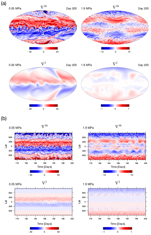
Figure 9: Relative vorticity fields in Mollweide projection at $t=200$ for $p\in\{0.05,1.90\}$ from the T170L200 deep atmosphere simulations. The simulations are set up identically – except for their dissipation order, $\mathfrak{p}\in\{1,8\}$ (and their correspondingly adjusted viscosity coefficient $\nu_{2\mathfrak{p}}$). Red (blue) colour represents positive (negative) values of relative vorticity. Deep atmosphere flow fields are more zonal compared to shallow atmosphere flow fields at the $p$-levels common to both atmospheres (i.e. $p\in[0.0,0.1]$), particularly in the equatorial region and at the levels away from the $p_{\rm top}$. Also, the large-scale flow is now separately barotropic in two distinct vertical sub-regions, $0.05\ga p\ga 1$ and $1\ga p\ga 10$; in the latter region, the flow is much less zonal than in the former region. This general behaviour is independent of $\mathfrak{p}$. However, the amplitude of the equatorial jet (the roughly 60^∘–wide band of $\zeta$ with the transition in sign across the equator) is greater for higher $\mathfrak{p}$; here the jet amplitude is related to the gradient of $\zeta$ contours.

Thus far, we have laid focus on the convergence behaviour of a shallow atmosphere, for which $p_{\rm bot}$ is set to be 0.1. As mentioned in section 2, the planetary radius $R_{p}$ is typically measured out to this $p$-level on giant planets: importantly, it is also roughly the $p$-level at which the optical path length of visible and near infrared radiation, entering from the top, begins to reach unity (e.g. Irwin, 2009). For Jupiter, a $p_{\rm bot}$ range of 0.1 to 1.0 is common for studying the dynamics near the visible cloud deck level (e.g. Vasavada & Showman, 2005; Sánchez-Lavega et al., 2019). This is despite the expectation that the radiatively stratified region extends to a greater $p$-level (i.e. deeper in), with the actual value currently uncertain. For extrasolar planets, the choice of $p_{\rm bot}$ value is more arbitrary and arguable. However, we have observed that a number of atmospheric flow and general circulation properties of Jupiter-like extrasolar planets – including convergence – is independent of the value of $p_{\rm bot}$ (up to $p_{\rm bot}=20$). In this paper, we continue to emphasize the generic properties of convergence that apply to both shallow and deep atmospheres.

Because the existence – and, if so, the location of – a solid surface for giant planets is unknown, the vertical domain range of simulations is generally chosen based on the physical phenomenon of interest and the computational resources available. A natural, and physically instructive, choice in this situation is to set $p_{\rm bot}$ to the level where there is a sharp change of vertical gradient or a jump in the basic stratification (e.g. laterally- and temporally-averaged Brunt-Väisälä frequency or density). Unfortunately, information on the detailed basic stratification structure is also unavailable. Formally, because of the restriction to the large scales imposed by the hydrostatic balance condition, equations (1) are strictly valid only for the stably-stratified radiative region, which overlies the unstably-stratified convective region. On large parts of the day side, the boundary between these two stability regions could be located at a depth greater than $p=0.1$ because of the intense irradiation from the planet’s host star. The precise depth depends on $\lambda$ and $\phi$. Simple, one-dimensional models predict a value for the sub-stellar point as large as $p\sim\!1000$ (e.g. Guillot & Showman, 2002).

In the present sub-section, we consider the deep atmosphere, in which $p_{\rm bot}$ is 1.0 or 10. Our discussion here centres mainly on the latter instantiation because, as pertains to convergence, there is no qualitative difference between simulations with $p_{\rm bot}\in\{0.1,1.0\}$. Quantitatively, the general flow pattern changes monotonically as $p_{\rm bot}$ increases from 0.1 to 1.0: modons become weaker and wider and the equatorial jet becomes more zonal, as $p_{\rm bot}\rightarrow 1$. The qualitatively-robust general behaviour is due to the strongly barotropic quality of the flow, which is intimately related to the setup used. Polichtchouk & Cho (2012) have previously reported quantitative changes in the baroclinicity when the $p_{\rm bot}$ is similarly increased in their idealised study of jet instability on hot-Jupiters. In that study, the (sectoral) wavenumber of the gravest unstable mode decreases slightly with a corresponding slight increase in the resulting flow’s zonality. Here the value of $p_{\rm top}$ in all the deep simulations is same as in the shallow atmosphere simulations, to facilitate unambiguous comparisons. A detailed discussion of the effects of vertical range variation will be provided elsewhere. We note that, in the employed setup, the depth at which the atmosphere ceases to be thermally forced is $p=1.0$; in addition, the forcing is very weak in the region $0.1\ga p>1$, compared to the levels near $p_{\rm top}$.

In light of the very high horizontal resolution requirement for convergence in $p_{\rm bot}=0.1$ simulations and the behaviour expected in $p_{\rm bot}=10$ simulations based on the similarity of $p_{\rm bot}\in\{0.1,1.0\}$ simulations, adequate vertical resolution for the $p_{\rm bot}=10$ deep atmosphere is at present computationally nearly prohibitive: we expect that effectively a series of long-duration, T341L2000 (or higher) simulations is needed for a robust assessment of full convergence for the atmosphere with $p_{\rm bot}=10$ (and even greater L for larger $p_{\rm bot}$). None the less, a ‘practical assessment’ can still be carried out with a reduced vertical range and/or layer density $\ell$ (i.e. L per MPa). As with the $p_{\rm bot}=1$ simulations, the $p_{\rm bot}=10$ simulations discussed in this paper (which are with up to T341L200 resolution and $t\in[0,500]$ duration) exhibit behaviours that are quantitatively different than the $p_{\rm bot}\in\{0.1,1.0\}$ simulations – particularly, when $\ell$ is high (e.g. $\ell\ga 200$) in the $p_{\rm bot}\in\{0.1,1.0\}$ simulations. This is in part due to the reduction of vertical resolution in the domain’s upper region (where the forcing is the strongest) in the $p_{\rm bot}=10$ simulations. However, we also observe weakening of the modons and strengthening of the overall flow’s zonality when L is increased while $\ell$ is held fixed (i.e. when layers are simply added at the bottom, keeping the vertical resolution in the domain’s upper region fixed). The latter behaviour is principally due to the aforementioned barotropic nature of the flow, in which the overall flow structure is in effect stretched vertically down to $p_{\rm bot}$, and the specified thermal forcing that must now drive a much larger mass of atmosphere than in the shallower atmospheres.

As mentioned, the horizontally (as well as vertically) under-resolved $p_{\rm bot}=10$ simulations are still revealing for convergence purposes. For example, consider Fig. 8. It shows the $\hat{\cal E}$ at $t=45$ from a series of simulations – all with $(p_{\rm bot},\mbox{L},\mathfrak{p})=(10,200,8)$, but with different T values. The spectra from the flow fields at the levels, $p=(5.0\times 10^{-3},5.0\times 10^{-1},1.0\times 10^{1})$, are shown in the (top, middle, bottom) panels in Fig. 8a. First, note the nearly identical spectra (up to the dissipation scale $n_{d}$ of each resolution given) for all T at $p=5.0\times 10^{-3}$; this match among the spectra here is actually slightly better than in the shallow atmosphere simulations (cf. Fig. 3). However, the spectra at the $p=\{5.0\times 10^{-1},1.0\times 10^{1}\}$ levels again exhibit spectral blocking (see e.g. the T170 spectra). This is very reminiscent of the behaviour already encountered in the shallow atmosphere simulations (cf. Fig. 3). Note also the much stronger oscillations in the lower $n$ part of the spectra at $p=5.0\times 10^{-1}$, which suggest a much stronger zonality at that $p$-level; such pronounced, ‘mid’-level feature is not present in the $p_{\rm bot}\in\{0.1,1.0\}$ simulations. Most importantly, as expected from what we have already observed in the shallow atmosphere case, the deep atmosphere simulations are not converged even at T341L200 resolution – particularly away from the top levels of the domain. This can be seen in Fig. 8b, in which the flow complexity clearly increases with T (and dynamism only with $\mbox{T}\geq 170$). In sum, we reiterate the following salient point: regardless of the vertical range of the modelled atmosphere, at least T341 horizontal resolution is needed for convergence.

Unsurprisingly, the above general behaviour with varying T is reproduced in the deep simulations with varying $\mathfrak{p}$. This is shown in Fig. 9, in which the instantaneous $\zeta$-fields (Fig. 9a) and their corresponding Hovmöller plots (Fig. 9b) are presented; here all the simulations in the figure are at T170L200 resolution. In the figure, several features are readily noticeable. First, as already discussed, deep atmosphere flow fields are more zonal compared to shallow atmosphere flow fields at the $p$-levels common to both atmospheres – particularly in the equatorial region, and at the levels away from the $p_{\rm top}$ (see Fig. 9a). Second, in $p_{\rm bot}=10$ simulations, the flow is also strongly barotropic, but roughly in two vertical sub-regions: $0.05\la p\la 1$ and $1\la p\la 10$. This is expected, given the specified forcing structure; it is also broadly consistent with behaviours reported in Thrastarson & Cho (2010) and Polichtchouk & Cho (2012). Third, in the latter region, the flow is generally much less zonal than in the former region. The azonal behaviour is supported by the lower boundary and is observed in all simulations, regardless of the $p_{\rm bot}$ value. The above features are independent of $\mathfrak{p}$. However, the field amplitude for $\mathfrak{p}=1$ is globally low compared to those from the simulations with higher $\mathfrak{p}$. Hence, the amplitude of the equatorial jet (the roughly 60^∘–wide band of $\zeta$ with the transition in sign across the equator) is greater for higher $\mathfrak{p}$.

The $\mathfrak{p}=8$ flow field is also distinct from the $\mathfrak{p}\in\{2,4\}$ flow fields (not shown), similar to what was observed in Fig. 6 for the shallow atmosphere. As in the shallow atmosphere simulations, the higher $\mathfrak{p}$ field contains many more small-scale flow structures. But, in the deep atmosphere simulations, the small-scale vortices are associated more strongly with a process of continuously peeling-off from the dynamic equatorial jet – rather than from the combined action of modon radiation and jet instability, seen in the shallow atmosphere simulations. Also clearly visible in the flow fields (but, importantly, not in the spectra) is the large-amplitude Rossby wave at the jet’s core (undulation of the $\zeta\rightarrow 0$ line in both of the $\mathfrak{p}=\{1,8\}$ simulations, at both of the $p$-levels shown). The undulations aids in the production of large-scale, as well as small-scale, vortices.

The flow of the deep atmosphere simulations also evolves very differently than that of the shallow atmosphere simulations. This can be readily seen in the Hovmöller plots shown in Fig. 9b. The duration in the plots is $t\in[175,200]$, well after equilibration of the bottom region (which occurs much later than in the shallow atmosphere simulations). In Fig. 9b, the difference in behaviours of $\mathfrak{p}\in\{1,8\}$ simulations seen in Fig. 9a persists in time. Here large-amplitude Rossby wave propagation can be seen more clearly (indicated by undulations of $\zeta$-amplitudes near the equator in time). In addition, the $\mathfrak{p}=8$ evolution appears to contain one or two more jets than in the $\mathfrak{p}=1$ evolution. In the latter, large time-scale variation of period $\sim$ 5 days can be seen at $p=0.05$, as well as shorter time-scale variations of period $\sim\!1/3$ day at both of the $p$-levels shown. For the modelled planet atmosphere, because ${\cal L_{R}}/R_{p}={\cal O}(1)$, where ${\cal L_{R}}\equiv(g{\cal H}/\Omega^{2})^{1/2}$ is the external Rossby deformation scale (e.g. Holton, 2004), the number of bands (jets) is expected to decrease over long time – especially at the greater $p$-level. This is because ${\cal L_{R}}$ is effectively the interaction length between the jets (see Cho & Polvani, 1996a, b; Cho et al., 2008).

We have also observed several additional features worthy of mention. First, little difference in the basic structure is discernible between the $\mathfrak{p}\in\{2,4\}$ evolutions, while the $\mathfrak{p}=1$ evolution is markedly different (most noticeably in the amplitude) compared to the other two evolutions; on the other hand, while the $\mathfrak{p}=8$ evolution is broadly similar to the $\mathfrak{p}\in\{2,4\}$ evolutions, vortices are smaller and the cross-equatorial flow is much stronger in the former. The latitudinal gradients are much sharper in the $\mathfrak{p}=8$ evolution as well; hence, we expect correspondingly sharper jets. After the initial ramp-up period, these features persist over the entire duration of the simulations (up to $t=500$). As discussed, T341L200 simulations with $\mathfrak{p}=8$ and vertical domain range $p\in[0,1]$ show a much more dynamic evolution, which is closer to the behaviour seen in Fig. 6 for a T341L20 simulation with range $p\in[0,0.1]$. Additionally, while the general jet behaviour is robust, the differences in the jet core (with span $\phi\la|\!\pm 30^{\circ}|$) and the jet flanks (located at $\phi\sim|\!\pm 30^{\circ}|$) is less pronounced in the T85L200 and T42L200 simulations (not shown), suggesting a transition similar to what was observed in the shallow atmosphere simulations at the T341 resolution (cf. section 3.2).

In summary, the non-convergence of simulations with up to T341L200 and $\mathfrak{p}=8$ as well as the behavioural trends laid out in the foregoing discussion together indicate convergence could be achieved at the next higher horizontal resolution – if the layer density $\ell$ is much greater (e.g. $\ell\sim 200$, in contrast to 20 above). Given this, we estimate at least T341L2000 resolution with $\mathfrak{p}=8$ is needed for a robust assessment of convergence (and preferably a resolution of T341L4000). Even with such a resolution, the simulations are not likely to be converged away from the top region of the modelled domain – as we have shown here in both the shallow and deep atmosphere context.

4 Conclusion

In this paper, we have summarised the main results from an in-depth exploration of convergence in extrasolar planet atmosphere flow simulations. Converged flow dynamics solutions are critical because they form the backbone for accurate modelling of other important (e.g. thermal, radiative and chemical) processes which directly affect observations and interpretations. In short, we have found that a horizontal resolution of T341 with a $\nabla^{16}$ hyperdissipation (roughly equivalent to at least a $2000\times 1000$ finite-difference grid, when solutions are smooth) and a concomitant vertical resolution of $\ell\!\sim\!200$ (i.e., $\sim$200 levels, or layers, per MPa), is minimally needed for convergence in hot-planet simulations: we suggest T341L4000. Crucially, this is because of the energetic small-scale vortices and waves, which naturally arise in the ageostrophic condition of the modelled planet atmosphere.

More broadly, this work presents several significant implications for extrasolar planet atmosphere studies. First, given that we have only invoked the conditions of stratification/density jump and ageostrophy, the results here also apply to simulations of close-in telluric planet atmospheres (ostensibly away from the boundary layer) – if similar forcing and initial condition are used. In fact, the results are arguably more appropriate for telluric planets in some ways because of the inescapable lower boundary required by discretization in simulation work. Of course, for such planets the boundary conditions should be augmented (e.g. with ‘no-slip’ and/or prescribed temperature at the bottom surface). Second, the results here also apply to studies that solve the full Navier–Stokes equations. This is because ageostrophy poses the same numerical difficulty (e.g. resolving small-scale flow structures) for both the primitive and Navier–stokes equations. Finally, the above resolution requirement suggests that current extrasolar planet atmosphere flow simulations are not converged. To the best of our knowledge, simulations employing the same (or similar) setup have thus far been performed with a lower resolution and dissipation order. Indeed, our results suggest that current simulations are erroneously converging to unphysical states: we recommend restricting the domain range and/or reformulating the equations for a more appropriate vertical coordinate.

The atmosphere has a number of properties that make the numerical solution of its governing equations especially challenging. Most obvious is the sphericity and anisotropy, the latter in both vertical (radial) and horizontal directions. That is, gravity and Coriolis acceleration impose a strong restraint in the vertical and meridional directions, respectively. The resulting stratifications induce the vertical length scales to be typically much smaller than the horizontal length scales and, to a much lesser extent, meridional scales to be smaller than the zonal scales. Hence, the ratio of horizontal to vertical model resolution and the lateral extent of the model domain should be carefully chosen to capture these anisotropies correctly. Because of the particularly strong vertical–horizontal anisotropy, atmospheric models are almost invariably constructed with a certain number of levels or layers in the vertical, with essentially the same horizontal grid or expansion basis structure at each level. Thus, we have discussed convergence naturally separated into horizontal and vertical issues.

Another fundamental challenge in modelling the atmosphere is its strong multi-scale property, in both space and time. In terms of spatial energy spectra, the largest scales are energetically dominant, but the spectra are shallow – implying that, whatever the resolution of an atmospheric model, there exists a significant dynamical variability near the resolution limit (which requires careful handling by numerical methods). Moreover, there is still the issue of unresolved scales, as the numerical models are still far from achieving realistic Reynolds number; this must be represented by a sub-grid model (here by hyper-viscosity). In addition, the atmosphere also supports dynamics with a huge range of timescales. Care is needed in modelling fast processes to ensure that the numerical solution is stable (in fact, convergence formally refers to a scheme/code which is both numerically consistent and stable). In contrast to geostrophic conditions, fast (gravity and sound) waves can be energetically much more significant in ageostrophic conditions. The chosen numerical method and code must be able to represent these features accurately. Also, certain properties of the atmosphere evolve slowly, either in a Lagrangian sense (e.g. the moisture content of an air parcel in the absence of condensation and evaporation) or in a global integral sense (e.g. the total angular momentum or energy of the atmosphere). These conservation properties must also be captured accurately. Note that some spectral blocking is almost inevitable in a long time integration of a nonlinear system (unless the dissipation is large).

A spectral method will conserve energy to a very high accuracy and will faithfully resolve a front or a shock with only two or three grid points across the structure. However, if these structures are poorly-resolved (or worse, under-resolved), its accuracy is no better than other methods. Energy-conserving and front-tracking schemes generate smooth solutions, but these may be far from the true solution. A turbulence calculation, such as one for extrasolar planet atmosphere, is almost by definition poorly resolved. In the present case, even dealiasing does not cure an under-resolved flow (when it is not suppressed by over-dissipation). For example, when a front forms, the solution is smooth for a finite time interval and then develops a jump discontinuity which the code is not able to resolve (leading to, inter alia, spectral blocking). Frontogenesis happens very rapidly once the modons grow to a reasonable size and strength – which occurs almost on a 1-day time-scale in the simulations. Hence, poorly-resolved simulations are predestined to fail convergence from the beginning of the simulation.

Finally, when the model top corresponds to the top of the atmosphere, it is reasonable to assume that there is no vertical mass flux across the upper boundary. This condition can be artificial, however, even when the upper boundary is formally placed at the top of the atmosphere, because of practical limitations on vertical resolution. At present, a simple but fully justifiable way of handling the upper boundary is not available. For a horizontally discrete model, the effective height of the surface at the model’s lower boundary may be higher than the actual height averaged over the grid box, and presents an additional challenge.

In this work, we have shown that a more numerically-suitable setup is needed (if not a more realistic one). Nominally, this means a more ‘balanced’ initial condition, which would mitigate the front and small-scale wave generation. Notably, what is not captured in lower resolution and lower order viscosity simulations (with the current setup) is the dominance of dynamic modons on close-in extrasolar planets and the modon’s influence in redistributing important fields (such as temperature and chemically- and radiatively-active species), as well observable variability of the planets. Here we have mainly focused on numerical convergence issues, as they relate to the flow dynamics. Hence, we have not discussed the effects of resolution and dissipation order on the temperature field. Indeed we have found that the flow and the temperature fields are intimately linked. This link is discussed in detail elsewhere, in two companion studies to the present work (Cho, Skinner & Thrastarson, submitted; Skinner & Cho, prep).

Data Availability

The data underlying this article will be shared on reasonable request to the corresponding author.

References

- Asselin (1972) Asselin R., 1972, Mon. Wea. Rev., 100, 487
- Bending, Lewis & Kolb (2013) Bending V. L., Lewis S. R., Kolb U., 2013, MNRAS, 428, 2874
- Boyd (2000) Boyd J. P., 2000, Chebyshev and Fourier Spectral Methods, 2nd ed., Dover, New York
- Byron & Fuller (1992) Byron F. W., Fuller R. W., 1992, Mathematics of Classical and Quantum Physics, Dover, New York
- Canuto et al. (1988) Canuto C., Hussaini M. Y., Quarteroni A., Zang T. A., 1988, Spectral Methods in Fluid Dynamics, Springer-Verlag, Berlin
- Cho & Polvani (1996a) Cho J. Y-K., Polvani L. M., 1996a, Phys. Fluids, 8, 1531
- Cho & Polvani (1996b) Cho J. Y-K., Polvani L. M., 1996b, Science, 273, 335
- Cho et al. (2003) Cho J. Y-K., Menou K., Hansen B. M. S., Seager S., 2003, ApJ, 587, L117
- Cho (2008) Cho J. Y-K., 2008, Atmospheric dynamics of tidally synchronized extrasolar planets, Phil. Trans. R. Soc. A, 366, 4477
- Cho et al. (2008) Cho J. Y-K., Menou K., Hansen B. M. S., Seager S., 2008, ApJ, 675, 817
- Cho, Polichtchouk & Thrastarson (2015) Cho J. Y-K., Polichtchouk I., Thrastarson H. Th., 2015, MNRAS, 454, 3423
- Cho et al. (2019) Cho J. Y-K., Thrastarson H. Th., Koskinen T. T., Read P. L., Tobias S. M., Moon W., Skinner J. W., 2019, Exoplanets and the Sun in Galperin B. & Read P. L. eds., Zonal Jets: Phenomenology, Genesis, and Physics. Cambridge University Press, Cambridge, p. 104
- Dobbs-Dixon & Lin (2008) Dobbs-Dixon I., Lin D. N. C., 2008, ApJ, 673, 513
- Dobbs-Dixon & Agol (2013) Dobbs-Dixon I., Agol E., 2013, MNRAS, 435, 3159
- Durran (2010) Durran D. R., 2010, Numerical Methods for Fluid Dynamics with Applications to Geophysics, 2nd ed., Springer, New York
- Eliasen et al. (1970) Eliasen E., Machenhauer B., Rasmussen E., 1970, Report No. 2, Inst. Teoretisk Meteorologi, Copenhagen Univ.
- Gottlieb & Orszag (1977) Gottlieb D., Orszag S. A., 1977, Numerical Analysis of Spectral Methods: Theory and Applications, SIAM, Philadelphia
- Guillot & Showman (2002) Guillot T., Showman A. P., 2002, A&A, 385, 156
- Hamilton & Ohfuchi (2008) Hamilton K., Ohfuchi W., 2008, High Resolution Numerical Modelling of the Atmosphere and Ocean, Springer, New York
- Heng, Menou & Phillipps (2011) Heng K., Menou K., Phillipps P. J., 2011, MNRAS, 413, 2380
- Holton (2004) Holton J. R., 2004, An Introduction to Dynamic Meteorology, 4th ed., Academic Press, San Diego
- Irwin (2009) Irwin P. G. J., 2009, Giant Planets of Our Solar System, 2nd ed., Praxis, Chichester
- Kreyszig (1978) Kreyszig E., 1978, Introductory Functional Analysis with Applications, Academic Press, San Diego
- Lauritzen et al. (2011) Lauritzen P. H., Jablonowski C., Taylor M. A., Nair R. D., 2011, Numerical Techniques for Global Atmospheric Models, Springer, Heidelberg
- Liu & Showman (2013) Liu B., Showman A. P., 2013, ApJ, 770, 42
- Mayne et al. (2014) Mayne N. J. et al., 2014, A&A, 561, 24
- Mendonça et al. (2016) Mendonça J. M., Grimm S. L., Grosheintz L., Heng K., 2016, ApJ, 829, 115
- Mendonça et al. (2018) Mendonça, J. M. et al., 2018, ApJ, 869, 107
- Menou (2020) Menou K., 2020, MNRAS, 493, 5038
- Orszag (1970) Orszag A., 1970, J. Atmos. Sci., 27, 890
- Orszag (1971) Orszag A., 1971, J. Atmos. Sci., 28, 1074
- Polichtchouk & Cho (2012) Polichtchouk I., Cho J. Y-K., 2012, MNRAS, 424, 1307
- Polichtchouk et al. (2014) Polichtchouk I., Cho J. Y-K., Watkins C., Thrastarson H. Th., Umurhan O. M., de la Torre Juárez M., 2014, Icarus, 229, 355
- Rivier, Loft & Polvani (2002) Rivier L., Loft R., Polvani L. M., 2002, Mon. Wea. Rev., 130, 1384
- Robert (1966) Robert A., 1966, J. Met. Soc. Japan, 44, 237
- Salby (1996) Salby M. L., 1996, Fundamentals of Atmospheric Physics, Academic Press, San Diego
- Scott et al. (2004) Scott R. K., Rivier L., Loft R., Polvani L. M, 2004, NCAR Technical Note No. 456
- Sánchez-Lavega et al. (2019) Sánchez-Lavega A. et al., 2019, Gas Giants in Galperin B. & Read P. L. eds., Zonal Jets: Phenomenology, Genesis, and Physics. Cambridge University Press, Cambridge, p. 72
- Showman et al. (2008) Showman A. P., Cooper C. S., Fortney J. J., Marley M. S., 2008, ApJ, 682, 559
- Showman et al. (2009) Showman A. P., Fortney J. J., Lian Y., Marley M. S., Freedman R. S., Knutson H. A., Charbonneau D., 2009, ApJ, 699, 471
- Showman, Cho & Menou (2011) Showman A. P., Cho J. Y-K., Menou K., 2011, Atmospheric circulation of exoplanets in Seager, S. ed., Exoplanets. University of Arizona Press, Tucson, p. 544
- Skinner & Cho (submitted) Skinner J. W., Cho J. Y-K., MNRAS (submitted)
- Stern (1975) Stern M. E., 1975, J. Mar. Res., 33, 1
- Strikwerda (2004) Strikwerda J. C., 2004, Finite Difference Schemes and Partial Differential Equations, 2nd ed., Society for Industrial and Applied Mathematics, Philadelphia
- Tan & Komacek (2019) Tan X., Komacek T. D., 2019, ApJ, 866, 26
- Temperton (1992) Temperton C., SIAM J. Sci. Stat. Comp., 13, 676
- Thrastarson & Cho (2010) Thrastarson H. Th., Cho J. Y-K., 2010, ApJ, 716, 144
- Thrastarson & Cho (2011) Thrastarson H. Th., Cho J. Y-K., 2011, ApJ, 729, 117
- Vasavada & Showman (2005) Vasavada A. R., Showman A. P., 2005, Rep. Prog. Phys., 68, 1935