Data Assimilation Networks

Abstract

Data Assimilation (DA) aims at estimating the posterior conditional probability density functions based on error statistics of the noisy observations and the dynamical system. State of the art methods are sub-optimal due to the common use of Gaussian error statistics and the linearization of the non-linear dynamics. To achieve a good performance, these methods often require case-by-case fine-tuning by using explicit regularization techniques such as inflation and localization. In this paper, we propose a fully data driven deep learning framework generalizing recurrent Elman networks and data assimilation algorithms. Our approach approximates a sequence of prior and posterior densities conditioned on noisy observations using a log-likelihood cost function. By construction our approach can then be used for general nonlinear dynamics and non-Gaussian densities. As a first step, we evaluate the performance of the proposed approach by using fully and partially observed Lorenz-95 system in which the outputs of the recurrent network are fitted to Gaussian densities. We numerically show that our approach, without using any explicit regularization technique, achieves comparable performance to the state-of-the-art methods, IEnKF-Q and LETKF, across various ensemble size.

Journal of Advances in Modeling Earth Systems (JAMES)

NVIDIA / ANITI, Toulouse, France Université de Toulouse / ANITI, Toulouse, France CERFACS / ANITI, Toulouse, France

Sixin Zhangsixin.zhang@irit.fr

We propose a general framework Data Assimilation Networks (DAN) based on an extended Elman Network for Bayesian Data Assimilation.

We show that DAN can achieve optimal prior and posterior density estimations by optimizing likelihood-based objective functions.

Numerically DAN achieve comparable performance to EnKF methods on Lorenz-95 system, without using explicit regularization such as localization or inflation.

Plain Language Summary

Data Assimilation (DA) aims at forecasting the state of a dynamical system by combining information coming from the dynamics and noisy observations. Bayesian data assimilation uses the random nature of a system to predict its states in terms of probability density functions (pdfs). The calculation of these densities is difficult for non-linear dynamical systems. Practical algorithms compute limited statistics due to computational cost, but this results in sub-optimal DA algorithms which requires then the use of explicit regularization techniques to increase the performance of the algorithm.

With the advances in Machine Learning (ML) and deep learning, there has been significant increase in the research of using ML for data assimilation to decrease the computational cost, or to have better estimation of the state. In this paper, we propose a fully data driven algorithm to learn the prior and posterior pdfs conditioned on given observations. Our learning is based on a set of trajectories of the model and observations. It aims to correct the pdfs by optimizing likelihood-based loss functions in the sense of the Kullback-Leibler (KL) divergence. Numerical experiments show that we can obtain similar performance when compared with the IEnKF-Q and LETKF methods, without the need of localization and inflation techniques. These numerical results shows the potential advantage of ML based algorithms when the used practical algorithms are sub-optimal.

1 Introduction

1.1 Context

In Data Assimilation (DA), the time dependent state of a system is estimated using two models that are the observational model, which relates the state to physical observations, and the dynamical model, that is used to propagate the state along the time dimension [Asch . (2016)]. These models can be written as a Hidden Markov Model (HMM).

Observational and dynamical models are described using random variables that account for observation and state errors. Hence DA algorithms are grounded on a Bayesian approach in which observation realizations are combined with the above statistical models to obtain state predictive and posterior density sequences. This estimation is done in two recursive steps: the analysis updates a predictive density into a posterior one with an incoming observation; and the propagation updates a posterior density into a the next cycle predictive (or prior) density.

DA methods use additional assumptions or approximations to obtain closed expressions for the densities so that they can be handled by computers. Historically in the Kalman filter (KF) approach, statistical models are assumed to be Gaussian and the physical dynamics are assumed to be linear [Kalman (1960)]. Hence, the propagation and analysis steps consist in updating mean and covariance matrix of Gaussian densities. A correct estimation of the covariance matrices is crucial since they determine to what extent the predictive density will be corrected to match observations. In the Ensemble Kalman Filter (EnKF) approach, the covariance matrices are represented by a set of sampling vectors to reduce the computational cost of the filter [Evensen (2009)]. When EnKF is used with a small number of ensembles, the covariance matrix estimation becomes low-rank. This causes some spurious correlations in the covariance matrix which are filtered by using regularization techniques such as localization and inflation [Hamill . (2001), Houtekamer  Mitchell (2001), Asch . (2016)]. EnKF can be used for nonlinear dynamics, however due to the truncation of the statistics up to the second order, in the limit of large ensembles the EnKF filter solution differs from the solution of the Bayesian filter [Le Gland . (2011)], except for linear dynamics and Gaussian statistics. Hence, when using these methods for non-linear and non-Gaussian setting there are still open questions in achieving an optimal prediction error in the Bayesian setting.

In this paper, we propose a general supervised learning framework based on Recurrent Neural Network (RNN) for Bayesian DA to approximate a sequence of prior and posterior densities conditioned on noisy observations. Section 2 explains the sequential Bayesian DA framework with an emphasis on the time invariant structure in the Bayesian DA which is the key property for RNNs. The proposed approach, Data Assimilation Network (DAN), is then detailed in Section 3 which generalizes both the Elman Neural Network and the Kalman Filter. DAN approximates the prior and posterior densities by minimizing the log-likelihood cost function based on the information loss, related to the cross-entropy. The details of the cost function and the theoretical results for the optimal solution of the cost function are presented in Section 3.4. The practical aspects of the DAN including the architecture and computationally efficient training algorithm are given in Section 4. We then evaluate the performance of DAN by using fully and partially observed Lorenz-95 system with Gaussian prior and posterior densities in Section 5. The Lorenz-95 system is non-linear and it is often used as a first-step in meteorology to investigate potential applications of the proposed method to high-dimensional chaotic systems. We compare the performance of DAN with state-of-the-art EnKFs methods, IEnKF-Q and LETKF, in terms of root mean square errors, and we also provide the stability analysis with respect to the initial condition and the forecast time-interval beyond the training range. Finally, we provide the conclusions in Section 6.

1.2 Related work

With the advances in machine learning and deep learning, there has been significant increase in the research of using ML to forecast the evolution of physical systems with a data-driven approach [Brunton . (2016), Rudy . (2017), Raissi . (2019), Raissi . (20171), Raissi . (20172), Li . (2020), Jia . (2021)]. Recently, this research has its significant impact on the design of advanced DA algorithms. We next outline three main directions that are related to our research in the hybridization of DA and ML approaches.

In a first direction, one addresses the traditional DA problem where the goal is to estimate the distribution of a state sequence $x_{t}$ conditioned on an observation sequence $y_{t}$, by using explicitly an underlying dynamical model $\mathcal{M}$. Harter2012 propose to use Elman Neural Network to learn the analysis equation of KF type algorithm where the dynamics are nonlinear. Their main aim is to reduce the computational complexity without affecting the accuracy. McCabe21 focus on the learning of the analysis equation within an EnKF framework. They propose the Amortized Ensemble Filter which aims to improve existing EnKF algorithms by replacing the EnKF analysis equations with a parameterized function in the form of a neural network.

In a second direction, one aims to learn an unknown dynamical model $\mathcal{M}$ from noisy observations of $y_{t}$. This direction is more ambitious compared to the first one as the dynamics to be learnt can be non-linear or even chaotic. Bocquet2019 propose to use the Bayesian data assimilation framework to learn a parametric $\mathcal{M}$ from sequences of observations $y_{t}$. The dynamical model is represented by a surrogate model which is formalized as a neural network under locality and homogeneity assumptions. Bocquet2020 extends this framework to the joint estimation of the state $x_{t}$ and the dynamical model $\mathcal{M}$ with a model error represented by a covariance matrix. They estimate the ensembles of the state by using a traditional Ensemble Kalman Smoother based on Gaussian assumption, and then with the given posterior ensemble they minimize for the dynamical model and its error statistics. Similarly, Brajard2020 propose an iterative algorithm to learn a neural-network parametric model of $\mathcal{M}$. With a fixed $\mathcal{M}$, it estimates the state $x_{t}$ using the observations $y_{t}$, and then uses the estimated state to optimize the parameters of $\mathcal{M}$. A related work is from Krishnan15, which introduces a deep KF to estimate the mean and the error covariance matrix in KF to model medical data, based on variational autoencoder [Girin . (2021)].

A third direction, which is what we consider in the present paper, is to estimate the distribution of a state sequence $x_{t}$ conditioned on a observation sequence $y_{t}$, without explicitly using the underlying dynamical model $\mathcal{M}$ in the propagation. This direction often uses training data in a supervised form of $(x_{t},y_{t})$. For instance, Fablet2021 propose a joint learning of the NN representation of the model dynamics and of the analysis equation albeit within a traditional variational data assimilation framework. A related work to learn a surrogate model is Revach_2022, which proposes a parametric KF to handle partially known model dynamics, replacing explicit covariance matrices by a parametric NN to estimate the model error. Pennyetal22 learns also a surrogate model, based on recurrent neural networks, by using only state sequence $(x_{t})$ which is then used in a deterministic EnKF framework.

All these approaches consider improving the DA methodologies which are based on an existing DA algorithm. In this work, we propose a fully data driven approach for Bayesian data assimilation without relying on any prior DA algorithm that can be sub-optimal in case of non-Gaussian error statistics and non-linear dynamics.

1.3 Notation

We denote a state random variable at time $t$ as $\boldsymbol{x}_{t}$ taking their values in some space $\mathbb{X}=\mathbb{R}^{n}$ of dimension $n$. An observation random variable at time $t$ is denoted by $\boldsymbol{y}_{t}$ taking its values in some space $\mathbb{Y}$ of dimension $d$ (often $\mathbb{R}^{d}$). We write a sequence of random variables $\boldsymbol{x}_{1},\cdots,\boldsymbol{x}_{t}$ as $\boldsymbol{x}_{1:t}$. A joint probability density of two sequence of random variables $\boldsymbol{x}_{1:t}$ and $\boldsymbol{y}_{1:t}$ with respect to the Lebesgue measure on the finite dimensional Euclidean space $\mathbb{X}^{t}\times\mathbb{Y}^{t}$ is written as $p(x_{1:t},y_{1:t})=p_{\boldsymbol{x}_{1:t},\boldsymbol{y}_{1:t}}(x_{1:t},y_{1:t})$. We denote the value (realization) of a random variable $\boldsymbol{x}$ as $x$. The set of pdfs over $\mathbb{X}$ is denoted by $\mathbb{P}_{\mathbb{X}}$. A conditional pdf for $\boldsymbol{x}_{t}$ conditioned on the value of $\boldsymbol{y}_{t}$, i.e. $\boldsymbol{y}_{t}=y_{t}$ is written as $p_{\boldsymbol{x}_{t}|\boldsymbol{y}_{t}}(\cdot|y_{t})$ $\in\mathbb{P}_{\mathbb{X}}$. Given a function $f(x)$ on a measurable space of $\mathbb{X}$ with measure $p$, we say $f(x)=0$ $p$-almost everywhere $x$ ($p$-a.e. $x$ in short), when there exists a measurable set $A$ with $p(A)=0$ such that $f(x)=0$ for all $x\not\in A$.

2 Sequential Bayesian Data Assimilation

In this section, we review the Bayesian optimal solution of sequential Bayesian data assimilation for an observed dynamical system and use its repetitive time-invariant structure to motivate the introduction of the DAN framework.

2.1 Sequential Bayesian Data Assimilation

Data assimilation aims to estimate the state of a dynamical process which is modeled by a discrete-time stochastic equation and observed via available instruments which can be modeled by another stochastic equation [Asch . (2016)]. These equations are given by the following system:

$$\boldsymbol{x}_{t} =\mathcal{M}\left(\boldsymbol{x}_{t-1}\right)+\boldsymbol{\eta}_{t},$$ (propagation equation) (1a)

$$\boldsymbol{y}_{t} =\mathcal{H}\left(\boldsymbol{x}_{t}\right)+\boldsymbol{\varepsilon}_{t},$$ (observation equation) (1b)

where $\mathcal{M}(\cdot)$ is the nonlinear propagation operator that acts on the model state random variable vector at time $t$, $\boldsymbol{x}_{t}\in\mathbb{X}$ and return the model state vector $\boldsymbol{x}_{t+1}\in\mathbb{X}$. $\mathcal{H}(\cdot)$ is the nonlinear observation operator that acts on the state random variable $\boldsymbol{x}_{t}$ and approximately returns the observation random variable $\boldsymbol{y}_{t}\in\mathbb{Y}$ at time t. Both of these steps may involve errors and they are represented by an additive model error, $\boldsymbol{\eta}_{t}$, and an additive observation error, $\boldsymbol{\varepsilon}_{t}$. For example, the observation operator may involve spatial interpolations, physical unit transformations and so on, resulting in measurement errors. We assume that these stochastic errors are distributed according to the pdf $p_{\boldsymbol{\eta}}$ and $p_{\boldsymbol{\varepsilon}}$ and they are i.i.d. along time, independent to the initial state $x_{1}$. Using these assumptions DA problem can be interpreted as a Hidden Markov Model [Carrassi . (2018)].

Given such a dynamical model, sequential Bayesian DA aims at quantifying the uncertainty over the system state each time an observation sample becomes available. Such an analysis starts by rewriting, under suitable mathematical assumptions, the DA system in terms of conditional probability density functions $p_{\boldsymbol{x}_{t}|\boldsymbol{x}_{t-1}}(\cdot|x_{t-1})\in\mathbb{P}_{\mathbb{X}}$ which represents (1a), and $p_{\boldsymbol{y}_{t}|\boldsymbol{x}_{t}}(\cdot|x_{t})\in\mathbb{P}_{\mathbb{Y}}$ which represents (1b). Using these densities, we can quantify the uncertainty of the state as a function of the observations. This can be done in two steps sequentially using the Bayesian framework: the analysis step and the propagation (forecast) step. Let $p_{t}^{b}:=p_{\boldsymbol{x}_{t}|\boldsymbol{y}_{1:t-1}}$ be the prior distribution of $\boldsymbol{x}_{t}$ given $\boldsymbol{y}_{1:t-1}$, and $p_{t}^{a}:=p_{\boldsymbol{x}_{t}|\boldsymbol{y}_{1:t}}$ be the posterior distribution of $\boldsymbol{x}_{t}$ given $\boldsymbol{y}_{1:t}$. The analysis step computes $p_{t}^{a}(\cdot|y_{1:t})\in\mathbb{P}_{\mathbb{X}}$ from $p_{t}^{b}(\cdot|y_{1:t-1})\in\mathbb{P}_{\mathbb{X}}$ based on Bayes rule,

$$p_{t}^{a}(\cdot|y_{1:t})=\frac{p_{\boldsymbol{y}_{t}|\boldsymbol{x}_{t}}(y_{t}|\cdot)\>p_{t}^{b}(\cdot|y_{1:t-1})}{p_{\boldsymbol{y}_{1:t-1}}(y_{1:t-1})}.$$ (2)

Here, $p_{\boldsymbol{y}_{t}|\boldsymbol{x}_{t}}(y_{t}|\cdot)$ is considered as a likelihood function of $x_{t}$, and $p_{\boldsymbol{y}_{1:t-1}}$ is a marginal distribution of observations. Similarly, the propagation step computes $p_{t+1}^{b}(\cdot|y_{1:t})$ from $p_{t}^{a}(\cdot|y_{1:t})$,

$$p_{t+1}^{b}(\cdot|y_{1:t}) =\int p_{\boldsymbol{x}_{t+1}|\boldsymbol{x}_{t}}(\cdot|x)p_{t}^{a}(x|y_{1:t})\mathrm{d}x.$$ (3)

The analysis and forecast steps are then repeated within a given number of cycles (time interval) in which the forecast step provides a prior density for the next cycle.

Performing the analysis and propagation steps in (2) and (3) with linear dynamics for the propagation operator $\mathcal{M}(\cdot)$ and the observation operator $\mathcal{H}(\cdot)$, and using a Gaussian assumption for the probabilities $p_{\boldsymbol{\varepsilon}}$ and $p_{\boldsymbol{\eta}}$ reduces to the well known Kalman filter (KF, [Kalman (1960)]). The challenge is that the calculation of the pdfs become intractable with nonlinear operators or non-Gaussian pdfs of the error terms. When the dynamics are nonlinear, ensemble type KFs such as Ensemble KF [Evensen (2009)] are widely used alternative methods, but when used with limited number of ensembles, they require additional remedies (see Section 3.3 for further discussions).

2.2 Time-invariant structure in the Bayesian Data Assimilation

We review the invariant structure of the Bayesian Data Assimilation (BDA) for the Hidden Markov Model (HMM) defined in Section 2.1, which is a key property to motivate the DAN framework. Following the i.i.d. assumptions that we have made on the errors in (1a) and (1b), the conditional pdfs $p_{\boldsymbol{x}_{t+1}|\boldsymbol{x}_{t}}$ and $p_{\boldsymbol{y}_{t}|\boldsymbol{x}_{t}}$ are time invariant, in the sense that for $t=1,2,\ldots$

$$p_{\boldsymbol{x}_{t+1}|\boldsymbol{x}_{t}}(u|v) =p_{\boldsymbol{x}_{2}|\boldsymbol{x}_{1}}(u|v)$$

$$p_{\boldsymbol{y}_{t}|\boldsymbol{x}_{t}}(y|v) =p_{\boldsymbol{y}_{1}|\boldsymbol{x}_{1}}(y|v)$$

for all $u,v\in\mathbb{X}$ and $y\in\mathbb{Y}$.

As a result, the conditional pdfs representing the HMM are time invariant in the following sense. The analysis step (2) can then be considered as a time invariant function, $a^{BDA}$, which operates on the prior cpdf, $p_{t}^{b}(\cdot|y_{1:t-1})\in\mathbb{P}_{\mathbb{X}}$ and a current observation, $y_{t}\in\mathbb{Y}$, and then return a posterior cpdf $p_{t}^{a}(\cdot|y_{1:t})\in\mathbb{P}_{\mathbb{X}}$:

$$p_{t}^{a}(\cdot|y_{1:t})=a^{BDA}\left[p_{t}^{b}(\cdot|y_{1:t-1}),y_{t}\right].$$

Similarly, according to (3), the propagation transformation can be considered as a time invariant function, $b^{BDA}$, that transforms a posterior pdf to a prior pdf,

$$p_{t+1}^{b}(\cdot|y_{1:t})=b^{BDA}\left[p_{t}^{a}(\cdot|y_{1:t})\right].$$

This presentation of the sequential BDA allows us to see the DA cycle as the composition of two time invariant transformations $a^{\mathrm{BDA}}$ and $b^{\mathrm{BDA}}$, i.e. each transformation is produced using the same update rule applied to the previous transformations. Exploiting this repetitive time invariant structure, corresponding to a chain of events, leads to a general framework named as the DAN based on recurrent neural networks (RNNs). We detail these ingredients of the DAN in Section 3 and Section 4.

3 Data Assimilation Networks (DAN)

In section 3.1 we present DAN, a general framework for DA, which generalizes traditional data assimilation algorithms such as the Kalman filter and the EnKF detailed in Section 3.2 and 3.3. Thanks to the repetitive structure of BDA, we propose in Section 3.4, a log-likelihood cost function based on the information loss to approximate conditional pdfs. Instead of calculating the posterior pdfs analytically, DAN aims to learn these pdfs by using sequences of $(x_{t},y_{t})$ generated from the HMM. We show theoretically that this framework allows one to handle nonlinear model dynamics and non-Gaussian error distributions where the Bayesian conditional pdfs are not necessarily Gaussian.

3.1 DAN framework

For a given set $\mathbb{S}$, DAN is defined as a triplet of transformations such that

$$a \in\mathbb{S}\times\mathbb{Y}\rightarrow\mathbb{S},\text{ (analyzer)}$$ (4a)

$$b \in\mathbb{S}\rightarrow\mathbb{S},\text{ (propagator)}$$ (4b)

$$c \in\mathbb{S}\rightarrow\mathbb{P}_{\mathbb{X}},\text{ (procoder)}$$ (4c)

The term “procoder” is a contraction of “probability coder” as the function $c$ transforms an internal representation into an actual pdf over $\mathbb{X}$. A representation of a DAN is given by Figure 1. When $S=\mathbb{P}_{\mathbb{X}}$ and $c$ is identity, this framework encompasses the transformation of $a^{\mathrm{BDA}}$ and $b^{\mathrm{BDA}}$ in the BDA as a special case. However, it includes also other DA algorithms such as Kalman Filter and Ensemble Kalman Filter. Such connections are detailed in Section 3.2 and 3.3.

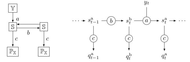
Figure 1: Representation of DAN. Left: scheme of DAN. Right: unrolled DAN along time interval.

One important ingredient of DAN as a general framework for cycled DA algorithms is the use of memory to transform prior and posterior densities from one cycle to the next one. In this respect, $\mathbb{S}$ can be interpreted as a memory space which is a vector space within the DAN framework. Considering DAN as a RNN with memory usage naturally make the link with the well-known Elman Network. This connection is detailed in Section 4.1.

As a recurrent neural network, we can unroll DAN into a sequence of transformations. Given an initial memory $s_{0}^{\mathrm{a}}\in\mathbb{S}_{0}$, and an observation trajectory $y_{1:T}\in\mathbb{Y}^{T}$, a DAN recursively outputs a predictive and a posterior sequence such that for $1\leq t\leq T$,

$$s_{t}^{b}\coloneqq b\left(s_{t-1}^{\mathrm{a}}\right),\quad s_{t}^{\mathrm{a}}\coloneqq a\left(s_{t}^{b},y_{t}\right)$$

$$q_{t}^{b}\coloneqq c\left(s_{t}^{b}\right),\quad q^{\mathrm{a}}_{t}\coloneqq c\left(s_{t}^{\mathrm{a}}\right).$$

This recursive application is represented in Figure 1. Note that $\{q_{t}^{b}\}_{t=1}^{T}$ and $\{q_{t}^{\mathrm{a}}\}_{t=1}^{T}$ are candidate conditional densities. This means that for a given sequence of observations $y_{1:t}=(y_{1},\cdots,y_{t})$, we have $q_{t}^{b}(\cdot|y_{1:t-1})\in\mathbb{P}_{\mathbb{X}}$ and $q_{t}^{\mathrm{a}}(\cdot|y_{1:t})\in\mathbb{P}_{\mathbb{X}}$. However, these candidate conditional densities are not required to be compatible by construction with a joint-distribution over $\mathbb{X}^{T}\times\mathbb{Y}^{T}$. As a consequence, we do not assume that there is some joint distribution $q(x_{1:T},y_{1:T})$ which induces the $q_{t}^{b}(\cdot|y_{1:t-1})$ and $q_{t}^{a}(\cdot|y_{1:t})$. However, as we shall see in Section 4, the construction of DAN using recurrent neural networks implicitly imposes some relationships between these candidate conditional densities.

3.2 The Kalman Filter as a DAN

In the original Kalman filter (KF) [Kalman (1960)], both the propagation operator $M$ and the observation operator $H$ are assumed to be affine. In this case, the analysis and propagation transformations preserve Gaussian pdfs that are easily characterized by their mean and covariance matrix. The analysis and propagation transformations then simplify to algebraic expressions on these pairs as we shall see in this section.

Suppose that the internal representation of a Gaussian pdf is formalized by the injective transformation, $c^{\mathrm{KF}}:\mathbb{Z}_{\mathbb{X}}\rightarrow\mathbb{G}_{\mathbb{X}}$,

$$c^{\mathrm{KF}}(s)=\mathcal{N}\left(\mu,\Sigma\right),$$

where $s\coloneqq(\mu,\Sigma)$, $\mu$ and $\Sigma$ being the mean and covariance matrix respectively and $\mathbb{Z}_{\mathbb{X}}$ is the set of mean and covariance matrix pairs over $\mathbb{X}$, $\mathbb{G}_{\mathbb{X}}$ is the set of Gaussian pdfs over $\mathbb{X}$. The KF analysis transformation is the function that transforms such a prior pair in $\mathbb{Z}_{\mathbb{X}}$ and an observation $y$ in $\mathbb{Y}$ into the posterior pair in $\mathbb{Z}_{\mathbb{X}}$, i.e. $a^{\mathrm{KF}}:\mathbb{Z}_{\mathbb{X}}\times\mathbb{Y}\rightarrow\mathbb{Z}_{\mathbb{X}}$, given by

$$a^{\mathrm{KF}}\left(\mu^{\mathrm{b}},\Sigma^{\mathrm{b}},y\right)=\left(\mu^{\mathrm{a}},\Sigma^{\mathrm{a}}\right)$$ (5)

with $\mu^{\mathrm{a}}=\mu^{\mathrm{b}}+\Sigma^{\mathrm{a}}H^{\mathrm{T}}R^{-1}\left(y-{H}\left(\mu^{\mathrm{b}}\right)\right)$. When the dimension of the observation $y_{t}$ is less or equal to the dimension of the state $x_{t}$, as an alternative we can obtain $\mu^{\mathrm{a}}=\mu^{\mathrm{b}}+K\left(y-{H}\left(\mu^{\mathrm{b}}\right)\right)$ and $\Sigma^{\mathrm{a}}=(I-KH)\Sigma^{\mathrm{b}}$ with $K=\Sigma^{\mathrm{b}}H^{\mathrm{T}}(H\Sigma^{\mathrm{b}}H^{\mathrm{T}}+R)^{-1}$. The mapping diagram for the analysis step of the KF is given by the diagram in Figure 2, which is a commutative diagram. We remind that a diagram is said to commute if any two paths between the same nodes compose to give the same map [Barr  Wells (1991)].

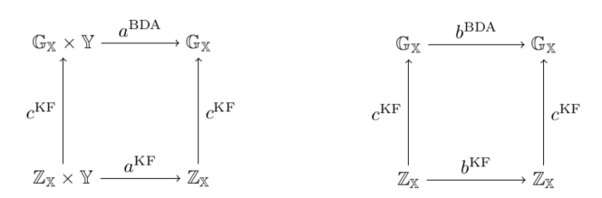
Figure 2: Kalman filter mapping diagram. Left: Commuting diagram for the KF analysis. Right: Commuting diagram for the KF propagation.

As well, the KF propagation transformation is the function that transforms a posterior pair in $\mathbb{Z}_{\mathbb{X}}$ into the next cycle prior in $\mathbb{Z}_{\mathbb{X}}$, i.e. $b^{\mathrm{KF}}:\mathbb{Z}_{\mathbb{X}}\rightarrow\mathbb{Z}_{\mathbb{X}}$, given by

$$b^{\mathrm{KF}}\left(\mu^{\mathrm{a}},\Sigma^{\mathrm{a}}\right)=\left(\mu^{\mathrm{b}},\Sigma^{\mathrm{b}}\right)$$ (6)

with $\Sigma^{\mathrm{b}}=M\Sigma^{\mathrm{a}}M^{\mathrm{T}}+Q,\,$ $Q$ being the model error covariance matrix and $\mu^{\mathrm{b}}=M\left(\mu^{\mathrm{a}}\right)$. The mapping diagram for the propagation step of the KF is given by the diagram in Figure 2, which is a commutative diagram.

Unfortunately, the linearity of $M$ and $H$ is rarely met in practice and covariance matrices may not be easy to store and manipulate in the case of large scale problems. A popular reduced rank approach is the ensemble Kalman filter that has proven effective in several large scale applications.

3.3 The Ensemble Kalman Filter as a DAN

In the Ensemble Kalman Filter (EnKF) [Evensen (2009)], statistics $\left(\mu,\Sigma\right)\in\mathbb{Z}_{\mathbb{X}}$ are estimated from an ensemble matrix $X\in\mathbb{X}^{m}=\mathbb{R}^{n\times m}$ having $m$ columns with the empirical estimators

$$\mu =Xu,$$ (7a)

$$\Sigma =XUX^{\mathrm{T}},$$ (7b)

where $u=\left(\frac{1}{m},\ldots,\frac{1}{m}\right)^{\mathrm{T}}\in\mathbb{R}^{m},U=\frac{I_{m}-m\times uu^{\mathrm{T}}}{m-1}\in\mathbb{R}^{m\times m}$ and $I_{m}\in\mathbb{R}^{m\times m}$ is the identity matrix [Fillion . (2020)]. Thus, the algebra over mean and covariance matrices pairs can be represented by operators on ensembles. In this approach nonlinear operators can be evaluated columnwise on ensembles and ensembles with few columns may produce low-rank approximations of large scale covariance matrices. Hence ensembles are an internal representation for the pdfs that are transformed by the function into a Gaussian pdf, $c^{\mathrm{E}nKF}:\mathbb{X}^{m}\rightarrow\mathbb{G}_{\mathbb{X}}$,

$$c^{\mathrm{E}nKF}(X)=\mathcal{N}\left(Xu,XUX^{\mathrm{T}}\right),$$ (8)

when the error covariance matrix $XUX^{\mathrm{T}}$ is full-rank, for instance when $m\geq n$. In the case when $m<n$, the error covariance matrix become rank deficient resulting in spurious correlations. In this rank-deficient case, we must select a different base measure where the Gaussian distribution is supported, by using generalized inverse of $XUX^{\mathrm{T}}$ [Rao (1973)].

The EnKF analysis transformation is the function that transforms such a prior ensemble $X_{\mathrm{b}}\in\mathbb{X}^{m}$ and an observation $y\in\mathbb{Y}$ into the posterior ensemble $X_{\mathrm{a}}\in\mathbb{X}^{m}$, $a^{\mathrm{EnKF}}:\mathbb{X}^{m}\times\mathbb{Y}\rightarrow\mathbb{X}^{m}$, given by

$$a^{\mathrm{EnKF}}\left(X_{\mathrm{b}},y\right)=X_{\mathrm{a}}\quad\text{with}\quad X_{\mathrm{a}}=X_{\mathrm{b}}+K\left(Y-Y_{\mathrm{b}}\right)$$ (9)

where $K=X_{\mathrm{b}}UY_{\mathrm{b}}^{\mathrm{T}}\left(Y_{\mathrm{b}}UY_{\mathrm{b}}^{\mathrm{T}}+R\right)^{-1}\in\mathbb{R}^{n\times d}$ is the ensemble Kalman gain, $Y_{\mathrm{b}}=\mathcal{H}\left(X_{\mathrm{b}}\right)\in\mathbb{Y}^{m}$ and $Y\in\mathbb{Y}^{m}(=\mathbb{R}^{d\times m})$ is a column matrix with $m$ samples of $\mathcal{N}\left(y,R\right)$.

As well, the EnKF propagation transformation is the function that transforms a posterior ensemble $X_{\mathrm{a}}\in\mathbb{X}^{m}$ into the next cycle prior ensemble $X_{\mathrm{b}}\in\mathbb{X}^{m}$, $b^{\mathrm{EnKF}}:\mathbb{X}^{m}\rightarrow\mathbb{X}^{m}$, given by

$$b^{\mathrm{EnKF}}(X_{\mathrm{a}})=X_{\mathrm{b}}\quad\text{with}\quad X_{\mathrm{b}}=\mathcal{M}\left(X_{\mathrm{a}}\right)+W$$ (10)

where $W\in\mathbb{X}^{m}$ is a column matrix consisting of $m$ samples distributed according to the Gaussian pdf $\mathcal{N}\left(0_{n},Q\right)$.

In EnKF, as explained above the mean and the covariance matrix for the Gaussian pdf are calculated through ensembles and propagation is performed through the ensembles using nonlinear dynamics. For large-scale nonlinear systems, when one can use only a limited number of ensembles, the error covariance matrix become a rank deficient matrix. This leads to sub-optimal performance [Asch . (2016)] and may introduce errors during the propagation. For instance, spurious correlations may appear or ensembles may collapse. As a result, for a stable EnKF regularization techniques like localization and inflation needs to be applied [Hamill . (2001), Houtekamer  Mitchell (2001), Gharamti (2018)]. Localization consists in filtering out the long-distance spurious correlations in the error covariance matrix. It is not straightforward to find the optimal parameters for the localization, therefore some tuning is required. After filtering out these spurious correlations such that the analysis is updated by the local observations, there may be still problem with the use of limited ensembles along the propagation. These small errors may be problematic when they are accumulated through the cycles. This can still lead to filter divergence. A common solution is to inflate the error covariance matrix by an empirical factor slightly greater than one. The multiplicative inflation compensate errors due to a small size of ensembles and the approximate assumption of Gaussian distribution on the error statistics [Bocquet (2011)].

3.4 DAN log-likelihood cost function

In this section, we introduce a cost function which allows one to optimize the candidate conditional densities, i.e. $q_{t}^{\mathrm{a}}$ and $q_{t}^{\mathrm{b}}$, based on samples of $\boldsymbol{x}_{1:T}$ and $\boldsymbol{y}_{1:T}$. The distance between the target conditional densities $p_{t}^{b}$ and $p_{t}^{\mathrm{a}}$ and the candidate conditional densities $q_{t}^{b}$ and $q_{t}^{\mathrm{a}}$ are minimized in the sense of the information loss, related to cross-entropy [Cover  Thomas (2005)].

Definition 1 (log-likelihood cost function).

Assume $q=(q^{b}_{t},q^{\mathrm{a}}_{t})_{t=1}^{T}\in\mathbb{P}=\left(\Pi_{t=1}^{T}\mathbb{Y}^{t-1}\rightarrow\mathbb{P}_{\mathbb{X}}\right)\times\left(\Pi_{t=1}^{T}\mathbb{Y}^{t}\rightarrow\mathbb{P}_{\mathbb{X}}\right)$ such that the following log-likelihood cost function is well-defined (i.e. for each $t\geq 1$, the Lebesgue integral with respect to $x_{1:t}$ and $y_{1:t}$ exists)

$$\mathcal{J}_{t}(q_{t}^{b},q_{t}^{\mathrm{a}})\coloneqq-\int\left[\ln q^{b}_{t}(x_{t}|y_{1:t-1})+\ln q^{\mathrm{a}}_{t}(x_{t}|y_{1:t})\right]p(x_{1:t},y_{1:t})\mathrm{d}x_{1:t}\mathrm{d}y_{1:t}.$$ (11)

The total log-likelihood cost function is defined as

$$\mathcal{J}(q)\coloneqq\frac{1}{T}\sum_{t=1}^{T}\mathcal{J}_{t}(q_{t}^{b},q_{t}^{\mathrm{a}}).$$ (12)

The following results show that if $q\in\mathbb{P}$, the global optima of $\mathcal{J}$ is the Bayesian prior and posterior cpdf trajectories of the HMM.

Theorem 1.

Let $\bar{q}\in\arg\min_{q\in\mathbb{P}}\mathcal{J}(q)$, then $\forall t\in\{1,\cdots,T\}$, $\bar{q}_{t}^{b}(x|y_{1:t-1})=p_{t}^{b}(x|y_{1:t-1})$ for $p_{t}^{b}(\cdot|y_{1:t-1})$-a.e $x\in\mathbb{X}$ and $p$-a.e $y_{1:t-1}\in\mathbb{Y}^{t-1}$. Similarly, $\bar{q}_{t}^{\mathrm{a}}(x|y_{1:t})=p_{t}^{\mathrm{a}}(x|y_{1:t})$ for $p_{t}^{\mathrm{a}}(\cdot|y_{1:t})$-a.e $x\in\mathbb{X}$ and $p$-a.e $y_{1:t}\in\mathbb{Y}^{t}$.

Proof.

See A. ∎

Theorem 1 shows that the objective function of DAN can approximate the Bayesian prior and posterior cpdf when the candidate pdfs belong to a general functional class (i.e. $q\in\mathbb{P}$). However, the loss function $\mathcal{J}(q)$ can not be numerically computed without making the functional class more specific. As a common specific case, we next consider candidate conditional pdfs as the Gaussian pdfs.

Let $\mathbb{G}_{\mathbb{X}}$ be the set of Gaussian pdfs over $\mathbb{X}$, and $q\in\mathbb{G}=\left(\Pi_{t=1}^{T}\mathbb{Y}^{t-1}\rightarrow\mathbb{G}_{\mathbb{X}}\right)\times\left(\Pi_{t=1}^{T}\mathbb{Y}^{t}\rightarrow\mathbb{G}_{\mathbb{X}}\right)$. For each $J_{t}(q_{t}^{b},q_{t}^{\mathrm{a}})$ in Definition 1 to be well-defined, it is necessary to assume that the target prior and posterior distributions $p_{t}^{b}(\cdot|y_{1:t-1})$ and $p_{t}^{\mathrm{a}}(\cdot|y_{1:t})$ have first-order and second-order moments. Under these assumptions, Theorem 2 shows that using Gaussian pdfs, one can match the correct mean and covariance of the target prior and posterior cpdf.

Theorem 2.

Let $\bar{q}\in\arg\min_{q\in\mathbb{G}}\mathcal{J}(q)$, then $\forall t\in\{1,\cdots,T\}$, the mean and covariance of $\bar{q}_{t}^{b}(\cdot|y_{1:t-1})$ equals to the mean and covariance of $p_{t}^{b}(\cdot|y_{1:t-1})$ for $p$-a.e $y_{1:t-1}\in\mathbb{Y}^{t-1}$. Similarly, the mean and covariance of $\bar{q}_{t}^{a}(\cdot|y_{1:t})$ equals to the mean and covariance of $p_{t}^{a}(\cdot|y_{1:t})$ for $p$-a.e $y_{1:t}\in\mathbb{Y}^{t}$.

Proof.

See B. ∎

Theorem 2 indicates that DAN has the capacity to optimally capture non-linear dynamics in terms of first and second-order statistics. Note that here the optimality is defined with respect to the cost function (12). Contrary to KF-based approaches, DAN never uses Gaussian approximations in its internal computations. DAN fits the output of the recurrent neural network with Gaussian pdfs.

4 DAN construction and training algorithm

Having specified the cost function in the previous section, we are now going to discuss how to construct the components of $a,b,c$ in DAN in order to fit training data samples. To motivate the DAN construction, we first review its connection with the classical Elman network in Section 4.1. We then specify the construction of a DAN using recurrent neural networks in Section 4.2. Section 4.3 and 4.4 describe how to efficiently train the network.

4.1 Connection with Elman network

DAN can be interpreted as an extension of an Elman network (EN) [Elman (1990)] which is a basic structure of recurrent network. An Elman network is a three-layer network (input, hidden and output layers) with the addition of a set of context units. These context units provide memory to the network. Both the input units and context units activate the hidden units; the hidden units then feed forward to activate the output units [Elman (1990)]. A representation of an EN is given in Figure 3.

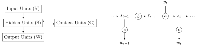
Figure 3: Representation of an Elman Network. Left: Scheme of an EN. Right: unrolled EN along time interval.

The context units make the Elman network able to process variable length sequences of inputs to produce sequences of outputs as shown in Figure 3. Indeed, given a new input $y_{t}\in\mathbb{Y}$ in the input sequence, the function $a$ updates a context memory from $\ell_{t-1}\in\mathbb{C}$ to a hidden state memory $s_{t}=a\left(\ell_{t-1},y_{t}\right)\in\mathbb{S}$. And the function $c$ decodes the hidden state memory into an output $w_{t}=c\left(s_{t}\right)\in\mathbb{W}$ in the output sequence. The updated hidden state memory is transferred to the context unit via a function $b$. In a way, the context memory of an Elman network is expected to gather relevant information from the past inputs to perform satisfactory predictions. The training process in machine learning will optimally induce how to manipulate the memory from data.

The similarity between DAN and EN can be made explicit with the analogy that the hidden layer is connected to the context units by the function $b$, which includes time propagation for DAN. In DAN the hidden unit memory $\mathbb{S}$ is considered as the same set as the context unit memory $\mathbb{C}$, and $c$ function decodes both the hidden and the context unit memory into a probability density function.

The EN can not perform DA operations in all its generality. For instance, EN can not make predictions without observations, that is estimating strict future states from past observations. This is because the function $a$ performs both the propagation and the analysis at once. In a way, the EN only produces posterior outputs and no prior outputs while the DAN produces prior or posterior outputs by applying the procoder $c$ before or after the propagator $b$ (see Figure 1 and Figure 3). DAN can also produce strict future predictions without observations by applying the propagator $b$ multiple times before applying the procoder $c$. Second, the DAN provides a probabilistic representation of the state i.e. an element in $\mathbb{P}_{\mathbb{X}}$ instead of an element in $\mathbb{X}$. Also, note that the compositions of $b$ and $c$ make a generalized propagation operator as it propagates in time probabilistic representations of the state rather than punctual realizations.

4.2 Construct DAN using Recurrent Neural networks (RNN)

We propose to use neural networks to construct a parameterized family of DANs. Let $\theta$ denote all the weights in neural networks, and the memory space $\mathbb{S}$ be a finite-dimensional Euclidean space. The parametric family of the analyzers and propagators are $L$-layer fully connected neural networks:

$$a_{\theta} :\quad\underbrace{\mathbb{S}\times\mathbb{Y}\rightarrow\cdots\rightarrow\mathbb{S}\times\mathbb{Y}}_{L\;times}\rightarrow\mathbb{S},$$ (13a)

$$b_{\theta} :\quad\underbrace{\mathbb{S}\rightarrow\cdots\rightarrow\mathbb{S}}_{L\;times},$$ (13b)

The construction of $a_{\theta}$ is built upon $L$ fully-connected layers with residual connections. It is based on the LeakyReLU activation function [Bing . (2015)] to improve the trainability when $L$ is large. For layer $\ell$, the input $v_{\ell-1}\in\mathbb{S}\times\mathbb{Y}$ is transformed into $v_{\ell}\in\mathbb{S}\times\mathbb{Y}$ by

$$v_{\ell}=v_{\ell-1}+\alpha_{\ell}\mathrm{LeakyReLU}\left(W_{\ell}v_{\ell-1}+\beta_{\ell}\right).$$ (14)

Taking a vector $v$ as its input, the LeakyReLU function outputs a vector $w$ of the same size. For the $i$-th element of $w$, $w_{i}=v_{i}$ if $v_{i}\geq 0$; $w_{i}=av_{i}$ if $v_{i}<0$, where $a$ is set to $0.01$ by default in our implementation based on Pytorch [Paszke . (2019)].

An extra linear layer is then applied to the output $v_{L}$ in order to compute a memory state as the output of $a_{\theta}$. The trainable parameters of $a_{\theta}$ are $(\alpha_{\ell},W_{\ell},\beta_{\ell})_{\ell\leq L}$ and the weight and bias in the linear layer. As illustrated in Figure 1, the input $a_{\theta}$ at time $t$ is a concatenation of $s_{t}^{b}$ and $y_{t}$, i.e. $v_{0}=(s_{t}^{b},y_{t})$. Similarly, $b_{\theta}$ is constructed from the same $L$ fully-connected layers as in (14) by using a different set of trainable parameters. The input of $b_{\theta}$ at time $t$ is set to $s_{t}^{a}$.

The procoder $c_{\theta}$ is specified with respect to the pdf choice of candidate conditional densities. For instance, for the Gaussian case studied in Theorem 2, $c_{\theta}$ can be defined as:

$$c_{\theta}:\quad\mathbb{S}\rightarrow\mathbb{R}^{n+\frac{n\left(n+1\right)}{2}}\rightarrow\mathbb{G}_{\mathbb{X}}$$ (15)

which is a linear layer from $\mathbb{S}$ to $\mathbb{R}^{n+\frac{n\left(n+1\right)}{2}}$, followed by a function that transforms the $n+\frac{n\left(n+1\right)}{2}$ dimensional vector into the mean and the covariance of a Gaussian distribution. This transformation is detailed in C.

4.3 Training and test loss from unrolled RNN

In order to train a DAN, we will unroll the RNN defined by $(a_{\theta},b_{\theta},c_{\theta})$ so as to define the training loss computed from $I$ i.i.d trajectories of $(\boldsymbol{x}_{1:T},\boldsymbol{y}_{1:T})$. We also define the test loss to evaluate the performance of training.

To be clear on how the states $s_{t}^{\mathrm{a}}$ and $s_{t}^{b}$ depend on $a_{\theta},b_{\theta}$ and a given trajectory $y_{1:t}$, we will denote the state (memory) at time $t$ informed by the data up to time $t\shortminus 1$ and generated using a $\theta$-parametric function as $s_{t|t\shortminus 1}^{b,\theta}$. Then we can rewrite $s_{t}^{b}$ and $s_{t}^{\mathrm{a}}$ more explicitly as:

$$s_{t|t\shortminus 1}^{b,\theta}=b_{\theta}\left(s_{t\shortminus 1|t\shortminus 1}^{\mathrm{a},\theta}\right),\quad and\quad s_{t|t}^{\mathrm{a},\theta}=a_{\theta}\left(s_{t|t\shortminus 1}^{b,\theta},y_{t}\right),$$ (16)

where $s_{0|0}^{\mathrm{a},\theta}=s_{0}$ is an initial memory of RNN independent of $\theta$. The procoder $c_{\theta}$ outputs the pdf

$$q_{t|t\shortminus 1}^{b,\theta}(\cdot|y_{1:t-1})=c_{\theta}\left(s_{t|t\shortminus 1}^{b,\theta}\right),\quad and\quad q_{t|t}^{\mathrm{a},\theta}(\cdot|y_{1:t})=c_{\theta}\left(s_{t|t}^{\mathrm{a},\theta}\right).$$ (17)

To define the training loss computed from the $I$ trajectories, we introduce a trajectory-dependent loss function which will be needed to define our online training strategy. Let $\left(x^{(i)}_{1:T},y^{(i)}_{1:T}\right)$ be the $i$-th trajectory, we write the loss function for the $i$-th trajectory as:

$$J_{t}^{(i)}\left(q_{t|t\shortminus 1}^{b,\theta},q_{t|t}^{\mathrm{a},\theta}\right)=-\log q_{t|t\shortminus 1}^{b,\theta}\left(x^{(i)}_{t}|y_{1:t-1}^{(i)}\right)-\log q_{t|t}^{\mathrm{a},\theta}\left(x^{(i)}_{t}|y_{1:t}^{(i)}\right).$$

The training loss is defined accordingly as a function of $\theta$,

$$\frac{1}{TI}\sum_{t=1}^{T}\sum_{i=1}^{I}J_{t}^{(i)}\left(q_{t|t\shortminus 1}^{b,\theta},q_{t|t}^{\mathrm{a},\theta}\right)$$ (18)

We define the test loss $J(\theta)$, as in (18), by using another $I$ independent trajectories of $(\boldsymbol{x}_{1:T},\boldsymbol{y}_{1:T})$. It allows one to evaluate how well a DAN learns the underlying dynamics of HMM beyond the training trajectories.

4.4 Online training algorithm: TBPTT

Direct optimization of the training loss in (18) is impractical for large-scale problems since to compute the gradient of the loss, with back-propagation through time, it requires a large computational graph that consumes a lot of memory  [Jaeger (2002)]. This limits the training data size $TI$ which, in turn, might lead to overfitting due to limited data. A workaround is to resort to gradient descent with truncated backpropagation through time (TBPTT, [Williams  Peng (1990), Williams  Zipser (1995)]). It is commonly used in the machine learning community to train recurrent neural networks [Tang  Glass (2018), Aicher . (2020)].

Starting from $\theta_{0}$, TBPTT is an online method which generates a sequence of model parameters $\theta_{k}$ for $k=1,2,\cdots,T$. Instead of computing the gradient of the loss (18) with respect $\theta$ which depends on time from $1$ to $T$, the idea of TBPTT is to truncate the computation at each iteration $k$ by considering only a part of the gradient from time $k-1$ to $k$. Each $\theta_{k}$ is obtained from $\theta_{k-1}$ based on the information of $I$ training trajectories $\{(x^{(i)}_{k},y^{(i)}_{k})\}_{i\leq I}$ on-the-fly.

More precisely, given the initial memories $\{\bar{s}_{0}^{(i)}\}_{i\leq I}$ and $\theta_{0}$, we update the memory

$$\bar{s}_{k}^{(i)}=a_{\theta_{k-1}}(b_{\theta_{k-1}}(\bar{s}^{(i)}_{k-1}),y^{(i)}_{k}),\quad k\geq 1$$

and then we perform the following gradient update,

$$\theta_{k+1}=\theta_{k}-\eta_{k}\frac{1}{I}\sum_{i=1}^{I}\nabla_{\theta}J^{(i)}_{k+1}(c_{\theta}\cdot b_{\theta}(\bar{s}_{k}^{(i)}),c_{\theta}\cdot a_{\theta}(b_{\theta}(\bar{s}_{k}^{(i)}),y_{k+1}^{(i)}))|_{\theta=\theta_{k}}$$ (19)

where $\eta_{k}$ is the learning rate. The learning rate is also called the step size in optimization. The gradient is computed over the $I$ training trajectories at time $k+1$. As a result, the optimization is not anymore limited in time due to computer memory constraints.

To adjust the learning rate $\eta_{k}$ adaptively, we apply the Adam optimizer [Kingma  Ba (2014)] to the gradient in (19). This simultaneously adjusts the updates of $\theta_{k}$ based on an average gradient computed from the gradients at previous steps.

5 Numerical experiments

In this section, we present results of DAN on the Lorenz-95 system [Lorenz (1995)] using the Gaussian conditional posteriors presented in Theorem 2. We first explain Lorenz dynamics in Section 5.1, and provide experimental details in Section 5.2. Then, Section 5.3 evaluates the effectiveness of the online training method TBPTT. Section 5.4 compares standard rmses performance of DAN to state-of-the-art DA methods IEnKF-Q and LETKF using a limited ensemble memory. We further study the robustness of DAN in terms of its performance on future sequences beyond the horizon $T$ of the training sequences, as well as its sensitivity to the initial distribution of each trajectory.

5.1 The Lorenz-95 system

The Lorenz-95 system introduced by Lore95 contains $n$ variables $x_{i},i=1,\ldots,n$ and is governed by the $n$ equations:

$$\frac{dx_{i}}{dt}=-x_{i-2}x_{i-1}+x_{i-1}x_{i+1}-x_{i}+F.$$ (20)

In Eq. (20) the quadratic terms represent the advection that conserves the total energy, the linear term represents the damping through which the energy decreases, and the constant term represents external forcing keeping the total energy away from zero. The $n$ variables may be thought of as values of some atmospheric quantity in $n$ sectors of a latitude circle.

In this study, we take $n=40$ and $F=8$ which results in some chaotic behaviour. The boundary conditions are set to be periodic, i.e., $x_{0}=x_{40}$, $x_{-1}=x_{39}$ and $x_{41}=x_{1}$. The equations are solved using the fourth-order Runge-Kutta scheme, with $\Delta t=0.05$ (a 6 hour time step).

5.2 Experiment setup

We study the performance of DAN when trained to map to Gaussian posteriors, i.e. the procoder $c$ function is given by (15). This is compared to two state-of-art baseline methods of EnKF: Iterative EnKF with additive model error (IEnKF-Q) [Sakov . (2018)] and Local Ensemble Transform Kalman filter (LETKF) [Hunt . (2007)].

A batch of $I$ trajectories of $x\in\mathbb{R}^{40}$ is simulated from the resolvant (propagation operator) $\mathcal{M}:\mathbb{R}^{40}\rightarrow\mathbb{R}^{40}$ of the $40$ dimensional Lorenz-95 system. To start from a stable regime, we use a burning phase which propagates an initial batch of states $\{x^{(i)}_{\mathrm{init}}\}_{i\leq I}$ for a fixed number of cycles. The initial states are drawn independently from $\mathcal{N}\left(3\times 1_{40},I_{40}\right)$. The operator $\mathcal{M}$ is then applied $10^{3}$ times (burning time) to the given initial batch of states [Sakov . (2018)]. The resulting states are taken as the initial state $x^{(i)}_{1}$.

After the burning phase, the Gaussian propagation errors $\{\eta^{i}_{t}\}$, sampled independently from $\mathcal{N}\left(0_{40},0.01\times I_{40}\right)$, are added to each subsequent propagation to get the state trajectories

$$x^{(i)}_{t+1} =\mathcal{M}\left(x^{(i)}_{t}\right)+\eta^{(i)}_{t},$$

Then the Gaussian errors $\varepsilon^{(i)}_{t+1}$, sampled independently from $\mathcal{N}\left(0_{40},I_{40}\right)$, are added to the observation operator evaluations to get a training batch of observation trajectories

$$y^{(i)}_{t+1} =\mathcal{H}\left(x^{(i)}_{t+1}\right)+\varepsilon^{(i)}_{t+1}.$$

In the numerical experiments we consider two cases for the observation network: (1) fully observed, i.e. $\mathcal{H}$ is taken to be the identity operator $I$, and (2) partially observed, i.e. $\mathcal{H}$ is taken as a uniform selection operator $H_{0}$. For any $40$-dimensional vector $x$, the vector $H_{0}x$ preserves half of the grid of $x$, by removing even-indexed elements of $x$. It is left as a future work to study cases where $H$ is a nonlinear operator.

5.2.1 Setup of Baseline

The baseline methods, IEnKF-Q and LETKF, are implemented with explicit inflation or localization regularization in order to obtain a good estimation of the covariance matrix of Gaussian densities. Such regularization is often critical to the final performance of EnKF methods, and it often requires the tuning of hyper-parameters whenever the ensemble size $m$ is changed [Asch . (2016)].

To illustrate the sensitivity to the hyper-parameter tuning, we provide two set of experiments for LETKF: (1) (with case-by-case turning) The filter for each ensemble size is run with the best performance values provided in Table 1, found by a 2D grid search for each $m$, named as LETKF^∗. (2) (without case-by-case tuning) The filter for each ensemble is run with the best performance obtained at $m=20$, i.e. the grid search is only run for this $m$ and the obtained optimal hyper-parameters are used for all $m$. We name these experiments simply as LETKF.

We implemented the IEnKF-Q which uses only inflation regularization. This allows one to measure the effect of using both inflation and localization regularization in LETKF. We present results without case-by-case tuning across different number of ensembles for EnKF, i.e. $m\in\{5,10,20,30\}$. As we do not have localization in IEnKF-Q, we fine-tune the inflation hyper-parameter of this method at $m=20$ using grid-search. We find that on both fully observed and partially observed cases, a common inflation parameter 1.1 is close to be optimal among $\{1.0,1.02,1.03,1.04,1.07,1.08,1.09,1.1,1.2,1.3,2.0\}$, according to the time-averaged posterior (filtering) rmses (see the definition of the rmses in Section 5.4)

Experiments with the LETKF are performed by using an open source code: DAPPER [Raanes . (2022), version 1.2.1]. For each ensemble, we have performed 2D grid search. Localization radius is chosen from the set $\{1,2,4\}$ and the inflation hyper-parameter is chosen from the set $\{1.02,1.03,1.04,1.07,1.1\}$. We also use rotation after the analysis step which is shown to provide better performance for LETKF [Sakov  Oke (2008)]. The inflation and localization radius hyper-parameter values that provide the best performance according to the time-averaged posterior (filtering) rmses are given in Table 1.

m	5	10	20	30
inflation	$1.1$	$1.07$	$1.04$	$1.03$
local. radius	$1$	$2$	$4$	$4$

m	5	10	20	30
inflation	$1.1$	$1.04$	$1.03$	$1.02$
local. radius	$2$	$2$	$4$	$4$

Table 1: Optimal hyper-parameter values of LETKF across various ensemble size $m$ found by 2D grid search. Left: fully-observed case ($H=I$). Right: partially observed case ($H=H_{0}$).

5.2.2 Setup of DAN

To make DAN comparable to EnKF in terms of the used memory, we set the memory space $\mathbb{S}=\mathbb{R}^{m\times n}$. Similar to the results without case-by-case turning in LETKF and IEnKF-Q, hyper-parameters of DAN are only tuned at $m=20$, and then fixed across all $m$.

Across $m\in\{5,10,20,30\}$, DAN is trained with a batch size of $I=1024$ of training samples for $T=6\times 10^{5}$ cycles. The initial learning rate $\eta_{0}$ for the TBPTT is set to be $10^{-4}$. The initial memory $s_{0}$ of the RNN is set to be zero, while the initial parameter $\theta_{0}$ of the RNN is mostly set to be random. More precisely, we use the standard random initialization for the weights $(W,b)$ of each linear layer implemented in the Pytorch software. To train a neural network with a large number of layers $L$, we use the ReZero trick [Bachlechner . (2020)] which sets the initial weight $\alpha_{\ell}$ in (14) to be zero for each $\ell$. The functions $a$ and $b$ in the cost function of DAN are constructed by $L=20$ fully connected layers with residual connections (as detailed in Section 4).

5.3 Training performance of TBPTT

To show the effectiveness of the training method TBPTT specified in (19), we evaluate the test loss $J(\theta)$ using $I=1024$ i.i.d samples (defined in Section 4.3), on a sub-sequence of $\theta_{k}$. This allows one to access whether the online method is effective to minimize the total loss $\mathcal{J}(q)$ in (12). The training time of DAN grows with $T$ but it is not sensitive to the choice of $I$. This is because our current implementation runs on GPU graphics cards, which allows the computation over $I$ training samples to be in parallel. However, the sequential computation of TBPTT can not be done in parallel. One potential improvement of the running time is to use a modified version of TBPTT to improve the convergence rate, as suggested in [Chen . (2022), Algorithm 4.2].

The test loss $J(\theta_{k})$ changes over iteration $k$ are displayed in Figure 4. We observe that the minimal loss decreases as $m$ increases, suggesting that the performance of DAN is improved with the memory size. Moreover, we find that the test loss decreases during the training process, which shows that TBPTT implicitly minimizes the test loss $J(\theta)$. In theory, we expect this to happen for a suitable large memory size $m$ because it is proportional to the capacity of the neural networks used in DAN: a larger $m$ implies a better approximation of the posterior distributions due to the universal approximation property of neural networks. The trade-off is that a too large $m$ may lead to over-fitting (i.e. a large gap between the training loss and test loss), as we use only $I$ finite trajectories of $(x_{t},y_{t})$ in the training algorithm.

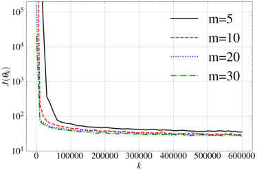
Figure 4: The test loss evaluated at training iterations $\theta_{k}$ of TBPTT, using various memory size $m$ in DAN.

5.4 Performance of DAN

After DAN is trained, new observation trajectories $y_{t}$ are generated from a new unknown state trajectory $x_{t}$. These testing observations together with a null initial memory vector are then given as input of the trained DAN in a test phase and its outputs are compared with the unknown state $x_{t}$.

To evaluate the accuracy of the trained DAN ($k=T$), we compute the accuracy of the mean $\mu_{t}^{\mathrm{a}}$ (resp. $\mu_{t}^{b}$) of $q_{t|t}^{\mathrm{a},\theta_{T}}(\cdot|y_{1:t})$ (resp. $q_{t|t-1}^{b,\theta_{T}}(\cdot|y_{1:t-1})$), evaluated on a test sequence $(x_{1:T},y_{1:T})$. A standard evaluation in DA is to compute rmses, i.e. for $1\leq t\leq T$, we compute the following normalized posterior and prior rmses,

$$R_{t}^{\mathrm{a}}=\frac{1}{\sqrt{n}}\|x_{t}-\mu_{t}^{{\mathrm{a}}}\|,\quad R_{t}^{b}=\frac{1}{\sqrt{n}}\|x_{t}-\mu_{t}^{b}\|$$

In Figure 5 and 6, we compare the averaged rmses of DAN with IEnKF-Q and LETKF when the ensemble size $m$ is smaller than the dimension $n$ of the state $x_{t}$. For DAN, we report an averaged rmses over $t$, computed at the parameter $\theta_{T}$ at the last step of training. These rmses are compared to the two baseline methods, IEnKF-Q and LETKF, over the same range of $t$. Recall that we use the same size $m$ to define the memory space $\mathbb{S}=\mathbb{R}^{m\times n}$ in DAN.

Let us first analyze the numerical results for the fully observed case. When $m$ is small, IEnKF-Q performs worse than DAN, due to sampling errors. Note that with the choice $F=8$ in the Lorenz-95 dynamics (Eq. (20)), the model has 13 positive and one neutral Lypapunov exponents, i.e. the dimension of the unstable-neutral subspace is 14 [Trevisan . (2010), Bocquet  Carrassi (2017), Sakov . (2018), Carrassi . (2022)]. Therefore, when the model is propagated through time, small perturbations grow along these directions [Carrassi . (2022)]. This explains why IEnKF-Q does not perform well when $m\leq 14$, as a result we need to apply localisation and inflation techniques to reduce these sampling errors. As expected, LETKF and LETKF*, in which localization and inflation techniques are applied with turned parameter values, performs much better than the IEnKF-Q. DAN performs similarly. When $m=5$, it is slightly better than LETKF* in the fully observed case. LETKF perfoms much worse than LETKF* and DAN, showing how sensitive the method is to the tuning of the inflation and localization hyper-parameters. When $m$ becomes closer to $n$ (e.g. $m=20,30$), we find that the posterior and prior rmses of DAN, IEnKF-Q, LETKF and LETKF^∗ are similar, with better results for LETKF^∗. This tendency of rmses as a function the ensemble size $m$ is strongly correlated with the smallest test loss achieved by DAN in Figure 4. We observe that for the partially observed case, conclusions are similar as well. These experiments clearly show that DAN can achieve a comparable performance without using EnKF-type regularization techniques.

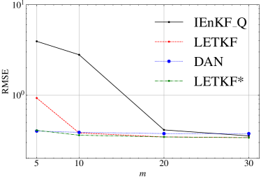
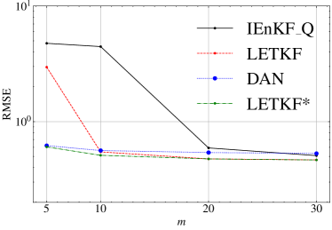
Figure 5: Time averaged posterior (filtering) rmses $\frac{1}{T}\sum_{t=1}^{T}R_{t}^{a}$ using various ensemble size $m$. Left: fully-observed case ($H=I$). Right: partially observed case ($H=H_{0}$). DAN, IEnKF-Q and LETKF are tuned at $m=20$; LETKF* is tuned at each $m$.

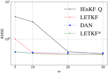
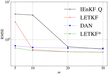
Figure 6: Time averaged prior (prediction) rmses $\frac{1}{T}\sum_{t=1}^{T}R_{t}^{b}$ using various ensemble size $m$. Left: fully-observed case ($H=I$). Right: partially observed case ($H=H_{0}$). DAN, IEnKF-Q and LETKF are tuned at $m=20$; LETKF* is tuned at each $m$.

5.5 Predictive performance and sensitivity to initialization

As DAN is trained on the time interval $t\leq T$, it remains important to evaluate its predictive performance by considering how well it performs for $t>T$. Such performance can be measured by the average rmses over $T+1\leq t\leq 2T$ instead of over $1\leq t\leq T$, evaluated using the trained model parameter ($\theta=\theta_{T}$). The posterior rmses for fully observed case are provided in Table 2. We find that the rmses over $T+1\leq t\leq 2T$ are close to those over $1\leq t\leq T$. This suggests that DAN has learnt the dynamics of the Lorenz system in order to perform well on future trajectories.

m	5	10	20	30
DAN	0.400	0.388	0.377	0.376

Table 2: Time averaged posterior (filtering) rmses $\frac{1}{T}\sum_{t=T+1}^{2T}R_{t}^{a}$ with various ensemble size.

All the earlier results are concerned of the performance of DAN under a fixed burning time. Using this burning time for the training of DAN, we further evaluate the rmses on test sequences which have a different burning time. It allows us to indirectly access how well recurrent structures inherited from the HMM are learnt. The results of the ensemble size $m=20$ are given in Table 3. It shows that the performance of DAN is not sensitive to the distribution of the test sample $x_{1}$ initialized over a wide range of burning time.

We remark that among all the simulations, there is always a relatively large error in $R_{t}^{a}$ and $R_{t}^{b}$ for small $t$ then it decreases very quickly (e.g. $m=20,\mbox{burning}=1000$, both $R_{t}^{a}$ and $R_{t}^{b}$ get close to a constant level when $t\geq 20$). This transition is needed for DAN to enter a stable regime because the initial memory of the RNN is set to zero.

burning time	$10^{1}$	$10^{3}$	$10^{5}$	$10^{7}$
DAN	0.376	0.376	0.377	0.377

Table 3: Time averaged posterior (filtering) rmses $\frac{1}{T}\sum_{t=1}^{T}R_{t}^{a}$ with various burning time at ensemble size $m=20$.

6 Conclusions

Based on the key observation that the analysis and propagation steps of DA consist in applying time-invariant transformations $a$ and $b$ that update the pdfs using incoming observations, we propose a general framework DAN which encompasses well-known state-of the art methods as special cases. We have shown that by optimizing suitable likelihood-based objective functions, the underlying posterior densities represented by these transformations have the capacity to approximate the optimal posterior densities of BDA. By representing $a$ and $b$ as neural networks, the estimation problem takes the form of the minimization of a loss with respect to the parameters of an extended Elman recurrent neural network. As a result, this general framework can be used for nonlinear dynamics and non-Gaussian error statistics.

In practice, we need to define the pdfs for the calculation of the loss function. As a first step and to be able to compare performance of DAN with the state-of-the-art ensemble methods, we perform numerical experiments with a procoder $c$ which outputs a Gaussian pdf. Our numerical results on a $40$-dimensional chaotic Lorenz-95 system show that when the ensemble size is small, DAN performs similarly compared to LETKF which includes regularization techniques such as localization and inflation. For large ensemble size, DAN has similar performance compared to IEnKF-Q and LETKF. It indicates that the DAN framework has the advantage of avoiding some problem-dependent numerical-tuning techniques. We also find that DAN is robust in terms of its predictive performance and its initialization.

Although we use a Gaussian approximation of the posterior densities in the procoder $c$, it can still happen that the memory space $\mathbb{S}$ may encode non-Gaussian information of the posterior distributions. To analyze why DAN can handle problems with nonlinear dynamics (even in other nonlinear dynamical systems) is left as a future study. From a practical point of view, DAN in its current form is not scalable to perform DA when the dimensionality $n$ is very large (e.g. in the order of $10^{9}$). To make DAN scalable, different training strategies [Chen . (2022), Penny . (2022)] will be considered in the future.

Open Research

All the results and data in this paper can be reproduced from a software which is available at https://gitlab.com/aniti-data-assimilation/dan_james. It can be cited at https://doi.org/10.5281/zenodo.7656199.

Appendix A Proof of Theorem 1

Proof.

According to (12), it is sufficient to derive the optimal solution of $\mathcal{J}_{t}(q_{t}^{b},q_{t}^{\mathrm{a}})$ for each $t$ independently. The proof is an application of the KL-divergence [Kullback  Leibler (1951)] to conditional probability densities. We re-write $\mathcal{J}_{t}(q_{t}^{b},q_{t}^{\mathrm{a}})$ as

$$\shortminus\int\ln q^{b}_{t}(x_{t}|y_{1:t\shortminus 1})p_{t}^{b}(x_{t}|y_{1:t\shortminus 1})p(y_{1:t\shortminus 1})dx_{t}\mathrm{d}y_{1:t\shortminus 1}-\int\ln q^{\mathrm{a}}_{t}(x_{t}|y_{1:t})p_{t}^{\mathrm{a}}(x_{t}|y_{1:t})p(y_{1:t})dx_{t}\mathrm{d}y_{1:t},$$ (21)

using the property $p(x_{t},y_{1:t-1})=p_{t}^{b}(x_{t}|y_{1:t\shortminus 1})p(y_{1:t\shortminus 1})$ and $p(x_{t},y_{1:t})=p_{t}^{a}(x_{t}|y_{1:t})p(y_{1:t})$. The first term in (21) can be written as a non-negative conditional relative entropy by including a constant conditional entropy term:

$$\int\left(\int\ln\frac{p^{b}_{t}(x_{t}|y_{1:t\shortminus 1})}{q^{b}_{t}(x_{t}|y_{1:t\shortminus 1})}p_{t}^{b}(x_{t}|y_{1:t\shortminus 1})dx_{t}\right)p(y_{1:t\shortminus 1})\mathrm{d}y_{1:t\shortminus 1}\geq 0.$$ (22)

We have equality in (22) if and only if $q^{b}_{t}(x|y_{1:t\shortminus 1})=p^{b}_{t}(x|y_{1:t\shortminus 1})$ for $p^{b}_{t}(\cdot|y_{1:t\shortminus 1})$-a.e $x$, and $p$-a.e. $y_{1:t\shortminus 1}$ (see a proof in [Kullback  Leibler (1951), Lemma 3.1] and [Bogachev (2007), Corollary 2.5.4]). Thus, the minimal solution is given by $\bar{q}_{t}^{b}$ as stated in the theorem. Similarly, the minimal solution of the second term (21) is given by the $\bar{q}_{t}^{\mathrm{a}}$ in the statement. ∎

Appendix B Proof of Theorem 2

Proof.

We shall only provide a proof for $\bar{q}_{t}^{b}(\cdot|y_{1:t-1})$ as the proof is similar for $\bar{q}_{t}^{a}(\cdot|y_{1:t})$. Let $\bar{p}^{b}_{t}(\cdot|y_{1:t-1})$ be the Gaussian distribution which has the mean and covariance of $p^{b}_{t}(\cdot|y_{1:t-1})$. Following the proof of Theorem 1, we can rewrite the first term, up to a constant, in (21) into

$$\int\left(\int\ln\frac{\bar{p}^{b}_{t}(x_{t}|y_{1:t-1})}{q^{b}_{t}(x_{t}|y_{1:t-1})}p_{t}^{b}(x_{t}|y_{1:t-1})dx_{t}\right)p(y_{1:t-1})\mathrm{d}y_{1:t-1}$$ (23)

This is an equivalent minimization problem because we have added a term of $\bar{p}_{t}^{b}$ which does not depend on $q_{t}^{b}$. By definition, $q^{b}_{t}(\cdot|y_{1:t-1})\in\mathbb{G}_{\mathbb{X}},\bar{q}^{b}_{t}(\cdot|y_{1:t-1})\in\mathbb{G}_{\mathbb{X}}$, the logarithm term in (23) is a quadratic function of $x_{t}$. As a consequence, we can rewrite (23) as

$$\int\left(\int\ln\frac{\bar{p}^{b}_{t}(x_{t}|y_{1:t-1})}{q^{b}_{t}(x_{t}|y_{1:t-1})}\bar{p}^{b}_{t}(x_{t}|y_{1:t-1})dx_{t}\right)p(y_{1:t-1})\mathrm{d}y_{1:t-1}\geq 0.$$ (24)

where we have replaced the density $p^{b}_{t}$ by $\bar{p}^{b}_{t}$ because they have the same first and second order moments. Note that the inner integral in (24) is the KL divergence between $\bar{p}^{b}_{t}$ and $q_{t}^{b}$, so its minimal solution $\bar{q}^{b}_{t}(\cdot|y_{1:t-1})$ equals almost surely to $\bar{p}^{b}_{t}(\cdot|y_{1:t-1})$. Therefore the mean and covariance of $\bar{q}^{b}_{t}(\cdot|y_{1:t-1})$ and $p^{b}_{t}(\cdot|y_{1:t-1})$ match for $p$-a.e. $y_{1:t-1}$. ∎

Appendix C Parameterization of DAN

We use the following parameterization of $\mu$ and $\Lambda$ to convert the vector $v\in\mathbb{R}^{n+\frac{n(n+1)}{2}}$ in (15) into a Gaussian distribution $\mathcal{N}(\mu,\Lambda\Lambda^{T})$. Let $v=(v_{0},\cdots,v_{n+n(n+1)/2-1})$, we set

$$\mu =\begin{pmatrix}v_{0}\\ \vdots\\ v_{n-1}\end{pmatrix}\in\mathbb{R}^{n},$$ (25a)

$$\Lambda =\begin{pmatrix}e^{v_{n}}&0&\cdots&0\\ v_{2n}&e^{v_{n+1}}&\ddots&\vdots\\ \vdots&\ddots&\ddots&0\\ v_{n+\frac{n\left(n+1\right)}{2}-1}&\cdots&v_{3n-2}&e^{v_{2n-1}}\end{pmatrix}\in\mathbb{R}^{\frac{n(n+1)}{2}}.$$ (25b)

The exponential terms in $\Lambda$ ensure the positive definiteness of $\Lambda\Lambda^{T}$. This can be easily implemented in Pytorch by using the module torch.distributions.multivariate_normal: MultivariateNormal(loc=$\mu$,scale_tril=$\Lambda$).

References

- Aicher \BOthers. (\APACyear2020) \APACinsertmetastarAicheretal20{APACrefauthors}Aicher, C., Foti, N\BPBIJ.\BCBL \BBA Fox, E\BPBIB. \APACrefYearMonthDay2020. \BBOQ\APACrefatitleAdaptively Truncating Backpropagation Through Time to Control Gradient Bias Adaptively Truncating Backpropagation Through Time to Control Gradient Bias.\BBCQ \BIn \APACrefbtitleProceedings of The 35th Uncertainty in Artificial Intelligence Conference Proceedings of the 35th uncertainty in artificial intelligence conference (\BVOL 115, \BPGS 799–808). \PrintBackRefs\CurrentBib
- Asch \BOthers. (\APACyear2016) \APACinsertmetastarAsch2016{APACrefauthors}Asch, M., Bocquet, M.\BCBL \BBA Nodet, M. \APACrefYear2016. \APACrefbtitleData assimilation: methods, algorithms, and applications Data assimilation: methods, algorithms, and applications. \APACaddressPublisherSIAM. \PrintBackRefs\CurrentBib
- Bachlechner \BOthers. (\APACyear2020) \APACinsertmetastarBachlechner2020{APACrefauthors}Bachlechner, T., Majumder, B\BPBIP., Mao, H\BPBIH., Cottrell, G\BPBIW.\BCBL \BBA McAuley, J. \APACrefYearMonthDay2020. \BBOQ\APACrefatitleReZero is All You Need: Fast Convergence at Large Depth ReZero is All You Need: Fast Convergence at Large Depth.\BBCQ \APACjournalVolNumPagesarXiv preprint arXiv:2003.04887. \PrintBackRefs\CurrentBib
- Barr \BBA Wells (\APACyear1991) \APACinsertmetastarpitts_1991{APACrefauthors}Barr, M.\BCBT \BBA Wells, C. \APACrefYearMonthDay1991. \BBOQ\APACrefatitleToposes, triples and theories. Grundlehren der mathematischen Wissenschaften, no. 278. Springer-Verlag, New York etc. 1985, xiii 345 pp. Toposes, triples and theories. grundlehren der mathematischen wissenschaften, no. 278. springer-verlag, new york etc. 1985, xiii 345 pp.\BBCQ \APACjournalVolNumPagesJournal of Symbolic Logic561340–341. {APACrefDOI} 10.2307/2274934 \PrintBackRefs\CurrentBib
- Bing \BOthers. (\APACyear2015) \APACinsertmetastarBing2015{APACrefauthors}Bing, X., Naiyan, W., Tianqi, C.\BCBL \BBA Mu, L. \APACrefYearMonthDay2015. \BBOQ\APACrefatitleEmpirical Evaluation of Rectified Activations in Convolutional Network Empirical Evaluation of Rectified Activations in Convolutional Network.\BBCQ \APACjournalVolNumPagesarXiv preprint arXiv:1505.00853. \PrintBackRefs\CurrentBib
- Bocquet (\APACyear2011) \APACinsertmetastarBocquet11{APACrefauthors}Bocquet, M. \APACrefYearMonthDay2011. \BBOQ\APACrefatitleEnsemble Kalman filtering without the intrinsic need for inflation Ensemble Kalman filtering without the intrinsic need for inflation.\BBCQ \APACjournalVolNumPagesNonlinear Processes in Geophysics185735–750. \PrintBackRefs\CurrentBib
- Bocquet \BOthers. (\APACyear2019) \APACinsertmetastarBocquet2019{APACrefauthors}Bocquet, M., Brajard, J., Carrassi, A.\BCBL \BBA Bertino, L. \APACrefYearMonthDay2019. \BBOQ\APACrefatitleData assimilation as a learning tool to infer ordinary differential equation representations of dynamical models Data assimilation as a learning tool to infer ordinary differential equation representations of dynamical models.\BBCQ \APACjournalVolNumPagesNonlinear Processes in Geophysics26143–162. \PrintBackRefs\CurrentBib
- Bocquet \BOthers. (\APACyear2020) \APACinsertmetastarBocquet2020{APACrefauthors}Bocquet, M., Brajard, J., Carrassi, A.\BCBL \BBA Bertino, L. \APACrefYearMonthDay2020. \BBOQ\APACrefatitleBayesian inference of chaotic dynamics by merging data assimilation, machine learning and expectation-maximization Bayesian inference of chaotic dynamics by merging data assimilation, machine learning and expectation-maximization.\BBCQ \APACjournalVolNumPagesFoundations of Data Science2155–80. \PrintBackRefs\CurrentBib
- Bocquet \BBA Carrassi (\APACyear2017) \APACinsertmetastarBocquetCarrassi2017{APACrefauthors}Bocquet, M.\BCBT \BBA Carrassi, A. \APACrefYearMonthDay2017. \BBOQ\APACrefatitleFour-dimensional ensemble variational data assimilation and the unstable subspace Four-dimensional ensemble variational data assimilation and the unstable subspace.\BBCQ \APACjournalVolNumPagesTellus A: Dynamic Meteorology and Oceanography6911304504. \PrintBackRefs\CurrentBib
- Bogachev (\APACyear2007) \APACinsertmetastarBogachev2007{APACrefauthors}Bogachev, V\BPBII. \APACrefYear2007. \APACrefbtitleMeasure Theory Measure Theory (\BNUM vol.1). \APACaddressPublisherSpringer Berlin Heidelberg. \PrintBackRefs\CurrentBib
- Brajard \BOthers. (\APACyear2020) \APACinsertmetastarBrajard2020{APACrefauthors}Brajard, J., Carassi, A., Bocquet, M.\BCBL \BBA Bertino, L. \APACrefYearMonthDay2020. \BBOQ\APACrefatitleCombining data assimilation and machine learning to emulate a dynamical model from sparse and noisy observations: a case study with the Lorenz 96 model Combining data assimilation and machine learning to emulate a dynamical model from sparse and noisy observations: a case study with the Lorenz 96 model.\BBCQ \APACjournalVolNumPagesArxiv preprint arXiv:2001.01520. \PrintBackRefs\CurrentBib
- Brunton \BOthers. (\APACyear2016) \APACinsertmetastarBruntonetal16{APACrefauthors}Brunton, S\BPBIL., Proctor, J\BPBIL.\BCBL \BBA Kutz, J\BPBIN. \APACrefYearMonthDay2016. \BBOQ\APACrefatitleDiscovering governing equations from data by sparse identification of nonlinear dynamical systems Discovering governing equations from data by sparse identification of nonlinear dynamical systems.\BBCQ \APACjournalVolNumPagesProceedings of the National Academy of Sciences113153932–3937. \PrintBackRefs\CurrentBib
- Carrassi \BOthers. (\APACyear2018) \APACinsertmetastarCarrassi2018{APACrefauthors}Carrassi, A., Bocquet, M., Bertino, L.\BCBL \BBA Evensen, G. \APACrefYearMonthDay2018. \BBOQ\APACrefatitleData assimilation in the geosciences: An overview of methods, issues, and perspectives Data assimilation in the geosciences: An overview of methods, issues, and perspectives.\BBCQ \APACjournalVolNumPagesWIREs Climate Change95e535. \PrintBackRefs\CurrentBib
- Carrassi \BOthers. (\APACyear2022) \APACinsertmetastarCarrassi2022{APACrefauthors}Carrassi, A., Bocquet, M., Demaeyer, J., Grudzien, C., Raanes, P.\BCBL \BBA Vannitsem, S. \APACrefYearMonthDay2022. \BBOQ\APACrefatitleData Assimilation for Chaotic Dynamics Data assimilation for chaotic dynamics.\BBCQ \BIn S\BPBIK. Park \BBA L. Xu (\BEDS), \APACrefbtitleData Assimilation for Atmospheric, Oceanic and Hydrologic Applications (Vol. IV) Data assimilation for atmospheric, oceanic and hydrologic applications (vol. iv) (\BPGS 1–42). \APACaddressPublisherChamSpringer International Publishing. \PrintBackRefs\CurrentBib
- Chen \BOthers. (\APACyear2022) \APACinsertmetastarchen2022autodifferentiable{APACrefauthors}Chen, Y., Sanz-Alonso, D.\BCBL \BBA Willett, R. \APACrefYearMonthDay2022. \BBOQ\APACrefatitleAutodifferentiable ensemble Kalman filters Autodifferentiable ensemble Kalman filters.\BBCQ \APACjournalVolNumPagesSIAM Journal on Mathematics of Data Science42801–833. \PrintBackRefs\CurrentBib
- Cover \BBA Thomas (\APACyear2005) \APACinsertmetastarCover2005{APACrefauthors}Cover, T\BPBIM.\BCBT \BBA Thomas, J\BPBIA. \APACrefYear2005. \APACrefbtitleElements of Information Theory Elements of Information Theory. \PrintBackRefs\CurrentBib
- Elman (\APACyear1990) \APACinsertmetastarElman1990{APACrefauthors}Elman, J\BPBIL. \APACrefYearMonthDay1990. \BBOQ\APACrefatitleFinding structure in time Finding structure in time.\BBCQ \APACjournalVolNumPagesCognitive Science142179–211. \PrintBackRefs\CurrentBib
- Evensen (\APACyear2009) \APACinsertmetastarEvensen2009{APACrefauthors}Evensen, G. \APACrefYear2009. \APACrefbtitleData Assimilation : The Ensemble Kalman Filter Data Assimilation : The Ensemble Kalman Filter. \APACaddressPublisherSpringer-Verlag Berlin Heidelberg. \PrintBackRefs\CurrentBib
- Fablet \BOthers. (\APACyear2021) \APACinsertmetastarFablet2021{APACrefauthors}Fablet, R., Chapron, B., Drumetz, L., Mémin, E., Pannekoucke, O.\BCBL \BBA Rousseau, F. \APACrefYearMonthDay2021. \BBOQ\APACrefatitleLearning Variational Data Assimilation Models and Solvers Learning Variational Data Assimilation Models and Solvers.\BBCQ \APACjournalVolNumPagesJournal of Advances in Modeling Earth Systems1310e2021MS002572. \PrintBackRefs\CurrentBib
- Fillion \BOthers. (\APACyear2020) \APACinsertmetastarFillionetal20{APACrefauthors}Fillion, A., Bocquet, M., Gratton, S., Gürol, S.\BCBL \BBA Sakov, P. \APACrefYearMonthDay2020. \BBOQ\APACrefatitleAn Iterative Ensemble Kalman Smoother in Presence of Additive Model Error An iterative ensemble kalman smoother in presence of additive model error.\BBCQ \APACjournalVolNumPagesSIAM/ASA Journal on Uncertainty Quantification81198-228. \PrintBackRefs\CurrentBib
- Gharamti (\APACyear2018) \APACinsertmetastarGharamti18{APACrefauthors}Gharamti, M\BPBIE. \APACrefYearMonthDay2018. \BBOQ\APACrefatitleEnhanced Adaptive Inflation Algorithm for Ensemble Filters Enhanced Adaptive Inflation Algorithm for Ensemble Filters.\BBCQ \APACjournalVolNumPagesMonthly Weather Review1462623–640. \PrintBackRefs\CurrentBib
- Girin \BOthers. (\APACyear2021) \APACinsertmetastarGirin21{APACrefauthors}Girin, L., Leglaive, S., Bie, X., Diard, J., Hueber, T.\BCBL \BBA Alameda-Pineda, X. \APACrefYearMonthDay2021. \BBOQ\APACrefatitleDynamical Variational Autoencoders: A Comprehensive Review Dynamical Variational Autoencoders: A Comprehensive Review.\BBCQ \APACjournalVolNumPagesFoundations and Trends® in Machine Learning151-21–175. \PrintBackRefs\CurrentBib
- Hamill \BOthers. (\APACyear2001) \APACinsertmetastarHamilletal01{APACrefauthors}Hamill, T\BPBIM., Whitaker, J\BPBIS.\BCBL \BBA Snyder, C. \APACrefYearMonthDay2001. \BBOQ\APACrefatitleDistance-Dependent Filtering of Background Error Covariance Estimates in an Ensemble Kalman Filter Distance-Dependent Filtering of Background Error Covariance Estimates in an Ensemble Kalman Filter.\BBCQ \APACjournalVolNumPagesMonthly Weather Review129112776–2790. \PrintBackRefs\CurrentBib
- Harter \BBA de Campos Velho (\APACyear2012) \APACinsertmetastarHarter2012{APACrefauthors}Harter, F\BPBIP.\BCBT \BBA de Campos Velho, H\BPBIF. \APACrefYearMonthDay2012. \BBOQ\APACrefatitleData Assimilation Procedure by Recurrent Neural Network Data Assimilation Procedure by Recurrent Neural Network.\BBCQ \APACjournalVolNumPagesEngineering Applications of Computational Fluid Mechanics62224–233. \PrintBackRefs\CurrentBib
- Houtekamer \BBA Mitchell (\APACyear2001) \APACinsertmetastarHoutekamerMitchell01{APACrefauthors}Houtekamer, P\BPBIL.\BCBT \BBA Mitchell, H\BPBIL. \APACrefYearMonthDay2001. \BBOQ\APACrefatitleA Sequential Ensemble Kalman Filter for Atmospheric Data Assimilation A Sequential Ensemble Kalman Filter for Atmospheric Data Assimilation.\BBCQ \APACjournalVolNumPagesMonthly Weather Review1291123–137. \PrintBackRefs\CurrentBib
- Hunt \BOthers. (\APACyear2007) \APACinsertmetastarHunt07{APACrefauthors}Hunt, B\BPBIR., Kostelich, E\BPBIJ.\BCBL \BBA Szunyogh, I. \APACrefYearMonthDay2007. \BBOQ\APACrefatitleEfficient data assimilation for spatiotemporal chaos: A local ensemble transform Kalman filter Efficient data assimilation for spatiotemporal chaos: A local ensemble transform kalman filter.\BBCQ \APACjournalVolNumPagesPhysica D: Nonlinear Phenomena2301112-126. \APACrefnoteData Assimilation \PrintBackRefs\CurrentBib
- Jaeger (\APACyear2002) \APACinsertmetastarJaeger2002{APACrefauthors}Jaeger, H. \APACrefYearMonthDay2002. \BBOQ\APACrefatitleTutorial on training recurrent neural networks, covering BPPT, RTRL, EKF and the echo state network approach Tutorial on training recurrent neural networks, covering BPPT, RTRL, EKF and the echo state network approach.\BBCQ \APACjournalVolNumPagesGMD-Forschungszentrum Informationstechnik5. \PrintBackRefs\CurrentBib
- Jia \BOthers. (\APACyear2021) \APACinsertmetastarJiaetal21{APACrefauthors}Jia, X., Willard, J., Karpatne, A., Read, J\BPBIS., Zwart, J\BPBIA., Steinbach, M.\BCBL \BBA Kumar, V. \APACrefYearMonthDay2021. \BBOQ\APACrefatitlePhysics-Guided Machine Learning for Scientific Discovery: An Application in Simulating Lake Temperature Profiles Physics-Guided Machine Learning for Scientific Discovery: An Application in Simulating Lake Temperature Profiles.\BBCQ \APACjournalVolNumPagesACM/IMS Trans. Data Sci.23. \PrintBackRefs\CurrentBib
- Kalman (\APACyear1960) \APACinsertmetastarKalman1960{APACrefauthors}Kalman, R\BPBIE. \APACrefYearMonthDay1960. \BBOQ\APACrefatitleA New Approach to Linear Filtering and Prediction Problems A New Approach to Linear Filtering and Prediction Problems.\BBCQ \APACjournalVolNumPagesJournal of Basic Engineering82135. \PrintBackRefs\CurrentBib
- Kingma \BBA Ba (\APACyear2014) \APACinsertmetastarKingma2014{APACrefauthors}Kingma, D.\BCBT \BBA Ba, J. \APACrefYearMonthDay2014. \BBOQ\APACrefatitleAdam: A Method for Stochastic Optimization Adam: A Method for Stochastic Optimization.\BBCQ \APACjournalVolNumPagesInternational Conference on Learning Representations. \PrintBackRefs\CurrentBib
- Krishnan \BOthers. (\APACyear2015) \APACinsertmetastarKrishnan15{APACrefauthors}Krishnan, R\BPBIG., Shalit, U.\BCBL \BBA Sontag, D. \APACrefYearMonthDay2015. \BBOQ\APACrefatitleDeep Kalman Filters Deep Kalman Filters.\BBCQ \APACjournalVolNumPagesarXiv preprint arXiv:1511.05121. \PrintBackRefs\CurrentBib
- Kullback \BBA Leibler (\APACyear1951) \APACinsertmetastarKL1951{APACrefauthors}Kullback, S.\BCBT \BBA Leibler, R\BPBIA. \APACrefYearMonthDay1951. \BBOQ\APACrefatitleOn Information and Sufficiency On Information and Sufficiency.\BBCQ \APACjournalVolNumPagesThe Annals of Mathematical Statistics22179–86. \PrintBackRefs\CurrentBib
- Le Gland \BOthers. (\APACyear2011) \APACinsertmetastarGland11{APACrefauthors}Le Gland, F., Monbet, V.\BCBL \BBA Tran, V\BHBID. \APACrefYearMonthDay2011. \BBOQ\APACrefatitleLarge sample asymptotics for the ensemble Kalman filter Large sample asymptotics for the ensemble Kalman filter.\BBCQ \BIn D. Crisan \BBA B. Rosovskii (\BEDS), \APACrefbtitleThe Oxford handbook of nonlinear filtering The Oxford handbook of nonlinear filtering (\BPGS 598–631). \APACaddressPublisherOxford University Press. \PrintBackRefs\CurrentBib
- Li \BOthers. (\APACyear2020) \APACinsertmetastarLietal20{APACrefauthors}Li, Z., Kovachki, N., Azizzadenesheli, K., Liu, B., Bhattacharya, K., Stuart, A.\BCBL \BBA Anandkumar, A. \APACrefYearMonthDay2020. \BBOQ\APACrefatitleFourier Neural Operator for Parametric Partial Differential Equations Fourier Neural Operator for Parametric Partial Differential Equations.\BBCQ \APACjournalVolNumPagesarXiv preprint arXiv:2010.08895. \PrintBackRefs\CurrentBib
- Lorenz (\APACyear1995) \APACinsertmetastarLore95{APACrefauthors}Lorenz, E\BPBIN. \APACrefYearMonthDay1995. \BBOQ\APACrefatitlePredictability: a problem partly solved Predictability: a problem partly solved.\BBCQ \BIn \APACrefbtitleSeminar on Predictability, 4-8 September 1995 Seminar on predictability, 4-8 september 1995 (\BVOL 1, \BPGS 1–18). \APACaddressPublisherShinfield Park, ReadingECMWF. \PrintBackRefs\CurrentBib
- McCabe \BBA Brown (\APACyear2021) \APACinsertmetastarMcCabe21{APACrefauthors}McCabe, J.\BCBT \BBA Brown, J. \APACrefYearMonthDay2021. \BBOQ\APACrefatitleLearning to Assimilate in Chaotic Dynamical Systems Learning to Assimilate in Chaotic Dynamical Systems.\BBCQ \BIn \APACrefbtitleAdvances in Neural Information Processing Systems Advances in neural information processing systems (\BVOL 34, \BPGS 12237–12250). \PrintBackRefs\CurrentBib
- Paszke \BOthers. (\APACyear2019) \APACinsertmetastarNEURIPS2019_9015{APACrefauthors}Paszke, A., Gross, S., Massa, F., Lerer, A., Bradbury, J., Chanan, G.\BDBLChintala, S. \APACrefYearMonthDay2019. \BBOQ\APACrefatitlePyTorch: An Imperative Style, High-Performance Deep Learning Library PyTorch: An Imperative Style, High-Performance Deep Learning Library.\BBCQ \BIn \APACrefbtitleAdvances in Neural Information Processing Systems 32 Advances in neural information processing systems 32 (\BPGS 8024–8035). \PrintBackRefs\CurrentBib
- Penny \BOthers. (\APACyear2022) \APACinsertmetastarPennyetal22{APACrefauthors}Penny, S\BPBIG., Smith, T\BPBIA., Chen, T\BHBIC., Platt, J\BPBIA., Lin, H\BHBIY., Goodliff, M.\BCBL \BBA Abarbanel, H\BPBID\BPBII. \APACrefYearMonthDay2022. \BBOQ\APACrefatitleIntegrating Recurrent Neural Networks With Data Assimilation for Scalable Data-Driven State Estimation Integrating Recurrent Neural Networks With Data Assimilation for Scalable Data-Driven State Estimation.\BBCQ \APACjournalVolNumPagesJournal of Advances in Modeling Earth Systems143e2021MS002843. \PrintBackRefs\CurrentBib
- Raanes \BOthers. (\APACyear2022) \APACinsertmetastardapper{APACrefauthors}Raanes, P\BPBIN., Chen, Y., Grudzien, C., Tondeur, M.\BCBL \BBA Dubois, R. \APACrefYearMonthDay2022. \APACrefbtitleDAPPER. Dapper. \APAChowpublishedhttps://github.com/nansencenter/DAPPER. \PrintBackRefs\CurrentBib
- Raissi \BOthers. (\APACyear2017\APACexlab\BCnt1) \APACinsertmetastarraissi2017physicsI{APACrefauthors}Raissi, M., Perdikaris, P.\BCBL \BBA Karniadakis, G\BPBIE. \APACrefYearMonthDay2017\BCnt1. \BBOQ\APACrefatitlePhysics Informed Deep Learning (Part I): Data-driven Solutions of Nonlinear Partial Differential Equations Physics Informed Deep Learning (Part I): Data-driven Solutions of Nonlinear Partial Differential Equations.\BBCQ \APACjournalVolNumPagesarXiv preprint arXiv:1711.10561. \PrintBackRefs\CurrentBib
- Raissi \BOthers. (\APACyear2017\APACexlab\BCnt2) \APACinsertmetastarraissi2017physicsII{APACrefauthors}Raissi, M., Perdikaris, P.\BCBL \BBA Karniadakis, G\BPBIE. \APACrefYearMonthDay2017\BCnt2. \BBOQ\APACrefatitlePhysics Informed Deep Learning (Part II): Data-driven Discovery of Nonlinear Partial Differential Equations Physics Informed Deep Learning (Part II): Data-driven Discovery of Nonlinear Partial Differential Equations.\BBCQ \APACjournalVolNumPagesarXiv preprint arXiv:1711.10566. \PrintBackRefs\CurrentBib
- Raissi \BOthers. (\APACyear2019) \APACinsertmetastarraissi2019physics{APACrefauthors}Raissi, M., Perdikaris, P.\BCBL \BBA Karniadakis, G\BPBIE. \APACrefYearMonthDay2019. \BBOQ\APACrefatitlePhysics-informed neural networks: A deep learning framework for solving forward and inverse problems involving nonlinear partial differential equations Physics-informed neural networks: A deep learning framework for solving forward and inverse problems involving nonlinear partial differential equations.\BBCQ \APACjournalVolNumPagesJournal of Computational Physics378686–707. \PrintBackRefs\CurrentBib
- Rao (\APACyear1973) \APACinsertmetastarRAO1973{APACrefauthors}Rao, C\BPBIR. \APACrefYear1973. \APACrefbtitleLinear Statistical Inference and its Applications: Second Editon Linear Statistical Inference and its Applications: Second Editon. \APACaddressPublisherJohn Wiley and Sons, inc. \PrintBackRefs\CurrentBib
- Revach \BOthers. (\APACyear2022) \APACinsertmetastarRevach_2022{APACrefauthors}Revach, G., Shlezinger, N., Ni, X., Escoriza, A\BPBIL., van Sloun, R\BPBIJ\BPBIG.\BCBL \BBA Eldar, Y\BPBIC. \APACrefYearMonthDay2022. \BBOQ\APACrefatitleKalmanNet: Neural Network Aided Kalman Filtering for Partially Known Dynamics KalmanNet: Neural Network Aided Kalman Filtering for Partially Known Dynamics.\BBCQ \APACjournalVolNumPagesIEEE Transactions on Signal Processing701532–1547. \PrintBackRefs\CurrentBib
- Rudy \BOthers. (\APACyear2017) \APACinsertmetastarRudyetal17{APACrefauthors}Rudy, S\BPBIH., Brunton, S\BPBIL., Proctor, J\BPBIL.\BCBL \BBA Kutz, J\BPBIN. \APACrefYearMonthDay2017. \BBOQ\APACrefatitleData-driven discovery of partial differential equations Data-driven discovery of partial differential equations.\BBCQ \APACjournalVolNumPagesScience Advances34e1602614. \PrintBackRefs\CurrentBib
- Sakov \BOthers. (\APACyear2018) \APACinsertmetastarSakov2018{APACrefauthors}Sakov, P., Haussaire, J\BHBIM.\BCBL \BBA Bocquet, M. \APACrefYearMonthDay2018. \BBOQ\APACrefatitleAn iterative ensemble Kalman filter in the presence of additive model error An iterative ensemble Kalman filter in the presence of additive model error.\BBCQ \APACjournalVolNumPagesQuarterly Journal of the Royal Meteorological Society1447131297–1309. \PrintBackRefs\CurrentBib
- Sakov \BBA Oke (\APACyear2008) \APACinsertmetastarSakovOke08{APACrefauthors}Sakov, P.\BCBT \BBA Oke, P\BPBIR. \APACrefYearMonthDay2008. \BBOQ\APACrefatitleImplications of the Form of the Ensemble Transformation in the Ensemble Square Root Filters Implications of the form of the ensemble transformation in the ensemble square root filters.\BBCQ \APACjournalVolNumPagesMonthly Weather Review13631042 - 1053. \PrintBackRefs\CurrentBib
- Tang \BBA Glass (\APACyear2018) \APACinsertmetastarHao2018{APACrefauthors}Tang, H.\BCBT \BBA Glass, J. \APACrefYearMonthDay2018. \BBOQ\APACrefatitleOn Training Recurrent Networks with Truncated Backpropagation Through Time in Speech Recognition On Training Recurrent Networks with Truncated Backpropagation Through Time in Speech Recognition.\BBCQ \APACjournalVolNumPagesarXiv preprint arXiv:1807.03396. \PrintBackRefs\CurrentBib
- Trevisan \BOthers. (\APACyear2010) \APACinsertmetastarTrevisanetal2010{APACrefauthors}Trevisan, A., D’Isidoro, M.\BCBL \BBA Talagrand, O. \APACrefYearMonthDay2010. \BBOQ\APACrefatitleFour-dimensional variational assimilation in the unstable subspace and the optimal subspace dimension Four-dimensional variational assimilation in the unstable subspace and the optimal subspace dimension.\BBCQ \APACjournalVolNumPagesQuarterly Journal of the Royal Meteorological Society136647487-496. \PrintBackRefs\CurrentBib
- Williams \BBA Peng (\APACyear1990) \APACinsertmetastarRonald90{APACrefauthors}Williams, R\BPBIJ.\BCBT \BBA Peng, J. \APACrefYearMonthDay1990. \BBOQ\APACrefatitleAn Efficient Gradient-Based Algorithm for On-Line Training of Recurrent Network Trajectories An Efficient Gradient-Based Algorithm for On-Line Training of Recurrent Network Trajectories.\BBCQ \APACjournalVolNumPagesNeural Computation24490–501. \PrintBackRefs\CurrentBib
- Williams \BBA Zipser (\APACyear1995) \APACinsertmetastarWilliamsZipser95{APACrefauthors}Williams, R\BPBIJ.\BCBT \BBA Zipser, D. \APACrefYearMonthDay1995. \BBOQ\APACrefatitleGradient-Based Learning Algorithms for Recurrent Networks and Their Computational Complexity Gradient-Based Learning Algorithms for Recurrent Networks and Their Computational Complexity.\BBCQ \BIn \APACrefbtitleBackpropagation: Theory, Architectures, and Applications Backpropagation: Theory, architectures, and applications (\BPGS 433–486). \APACaddressPublisherL. Erlbaum Associates Inc. \PrintBackRefs\CurrentBib