Geometric Constraints on Two-electron Reduced Density Matrices

Abstract

For many-electron systems, the second-order reduced density matrix (2-RDM) provides sufficient information for characterizing their properties of interests in physics and chemistry, ranging from total energy, magnetism, quantum correlation and entanglement to long-range orders. Theoretical prediction of the structural properties of 2-RDM is an essential endeavor in quantum chemistry, condensed matter physics and, more recently, in quantum computation. Since 1960s, enormous progresses have been made in developing RDM-based electronic structure theories and their large-scale computational applications in predicting molecular structure and mechanical, electrical and optical properties of various materials. However, for strongly correlated systems, such as high-temperature superconductors, transition-metal-based biological catalysts and complex chemical bonds near dissociation limit, accurate approximation is still out of reach by currently most sophisticated approaches. This limitation highlights the elusive structural feature of 2-RDM that determines quantum correlation in many-electron system. Here, we present a set of constraints on 2-RDM based on the basic geometric property of Hilbert space and the commutation relations of operators. Numerical examples are provided to demonstrate the pronounced violation of these constraints by the variational 2-RDMs. It is shown that, for a strongly correlated model system, the constraint violation may be responsible for a considerable portion of the variational error in ground state energy. Our findings provide new insights into the structural subtlety of many-electron 2-RDMs.

Introduction

In 1930, Paul Dirac introduced the idea of utilizing reduced density matrix (RDM) to approximate the properties of many-electron systems in order to avoid intractable computation of many-electron wave function.(Dirac, 2008) The research efforts in this direction led to the development of various electronic structure theories based on one- and two-electron RDMs (1-RDM and 2-RDM).(Husimi, 1940; Löwdin, 1955; Mayer, 1955; Hohenberg and Kohn, 1964; Kohn and Sham, 1965; Parr, 1989; Levy and Mel, 2005; Mardirossian and Head-Gordon, 2017; Verma and Truhlar, 2020; Coleman, 1963; Coleman and Yukalov, 2000; Mazziotti, 2007; Goedecker and Umrigar, 2000; Nagy, 2003; Sharma et al., 2008) Among these approaches, density functional theory (DFT) is most successful and popular.(Hohenberg and Kohn, 1964; Kohn and Sham, 1965; Parr, 1989; Mardirossian and Head-Gordon, 2017) In DFT, the ground-state energy is approximated by an energy functional of one-electron density (that is, the diagonal of 1-RDM), which provides sufficient accuracy with low computational cost for most of quantum physics and chemistry applications. A major challenge in DFT is to systematically improve energy functional approximation for describing strongly correlated systems.(Mardirossian and Head-Gordon, 2017; Verma and Truhlar, 2020; Sun et al., 2015; Ekholm et al., 2018; Isaacs and Wolverton, 2018)

In parallel, the approaches based on high-order RDM have been actively pursued aiming at the systems with strongly correlated electrons or nuclei.(Husimi, 1940; Löwdin, 1955; Mayer, 1955; Coleman, 1963; Valdemoro, 1996; Coleman and Yukalov, 2000; Mazziotti, 2007; Mayorga, 2018) In these approaches, the energy expression is exact. However, it is difficult to find sufficient constraints on an approximated RDM in order to ensure its correspondence to a many-electron wave function.(Coleman and Yukalov, 2000) In quantum chemistry, this problem is known as $N$-representability problem,(Coleman, 1963) a special case of quantum marginal problem in quantum information(Klyachko, 2006) . For strongly correlated systems, this problem may cause predicting erroneous bond dissociation barrier, and unphysical properties such as factional charges and factional spins.(Mihailović and Rosina, 1969; Ayers and Liu, 2007; Cohen et al., 2008; Aggelen et al., 2009; Nakata and Yasuda, 2009; Anderson et al., 2013; Ding and Schilling, 2020) Since the problem was formalized in early 1960s, substantial research efforts have been made to identify sufficiently stringent N-representability constraints and to implement them in practical computation. The progress has been steady but slow due to its challenging mathematical and computational nature.(Coleman, 1963; Coleman and Yukalov, 2000; Klyachko, 2006; Liu et al., 2007; Mazziotti, 2007; Li and Burke, 2018) With recent exciting development in quantum computing and information technologies, this problem is attracting more attention because of the key role of quantum marginals in quantum measurement and information processing.(McArdle et al., 2020; Higuchi et al., 2003; Higuchi, ; Klyachko, a; Liu et al., 2007; Cramer et al., 2010; Schilling, 2013; Mazziotti, 2016a; Rubin et al., 2018; Smart et al., 2019; Smart and Mazziotti, 2019; Takeshita et al., 2020)

Currently, most of nontrivial $N$-representability constraints are originated from two basic properties of a state in fermion Fock space: antisymmetric permutation(Klein and Kramling, 1969; Klein, 1969; Kryachko, 1981) and the fact that inner product of the state with itself is nonnegative. The symmetry property imposes an upper bound on the eigenvalues of 1-RDM (Pauli principle), and antisymmetric condition on electron and hole 2-RDM.(Coleman, 1963) A major breakthrough on the quantum marginal problem has been made by Klyachko utilizing representation theory of symmetric group, which leads a family of constraints on the eigenvalues of pure-state 1-RDM (Generalized Pauli constraints).(Borland and Dennis, 1972; Higuchi et al., 2003; Higuchi, ; Klyachko, a, 2006; Ruskai, 2007; Klyachko, b; Schilling, 2013; Schilling et al., 2018) Based on generalized Pauli constraints, pure-state constraints on 2-RDM have been proposed recently.(Mazziotti, 2016b)

The non-negativity inner product property requires any RDM to be Hermitian and positive semidefinite, which, for 2-RDM, implies a set of constraints known as: $D$, $Q$, $G$, $T1$, $T2$ and $T2^{\prime}$ conditions. The $D$, $Q$ and $G$ conditions were proposed by Coleman(Coleman, 1963), Garrod and Percus(Garrod and Percus, 1964) in early 1960s. In 1978, Erdahl discovered $T1$ and $T2$ conditions by introducing a clever idea to reduce the 3-RDM positive semidefinite conditions to a set of conditions on 1-RDM and 2-RDM.(Erdahl, 1978) The more restrictive $T2^{\prime}$ condition was reduced from the positive semidefinite condition on a variant of 3-RDM.(Zhao et al., 2004; Hammond and Mazziotti, 2005) Inspired by this idea, Mazziotti developed a systematic approach to deduce 2-RDM conditions from higher-order RDM constraints, and proved, in 2012, that inclusion of the whole set of deduced conditons sufficiently ensure a 2-RDM to be N-representable.(Mazziotti, 2012) However, the number of the deduced conditions increases exponentially with the many-body order of the RDM. It is not yet clear how the effectiveness of these conditions depends on the order increase.

At present, variational 2-RDM method is one of most promising high-order RDM approaches. In this approach, the positive semidefinite conditions can be implemented by either positive semidefinite programming (SDP)(Nakata et al., 2001) or nonlinear optimization(Mazziotti, 2004). For many molecular systems with up to 28 electrons, the accuracy of variational ground state energy is comparable to the high-level wavefunction-based method CCSD(T).(Zhao et al., 2004; Nakata et al., 2008) However, for the strongly correlated systems, such as 1D, quasi-2D and 2D Hubbard models(Hammond and Mazziotti, 2006; Nakata et al., 2008; Verstichel et al., 2013; Anderson et al., 2013; Rubin and Mazziotti, 2014), the Lipkin model(Hammond and Mazziotti, 2005), molecule chains(Mazziotti, 2004; Fosso-Tande et al., 2015; Mazziotti, 2016a), and the molecules near dissociation limit(Aggelen et al., 2009; van Aggelen et al., 2010; Nakata and Anderson, 2012; Nakata and Yasuda, 2009), the variatonal results are encouraging but still unsatisfactory. Evidently, more restrictive constraint is in demand to elucidate the intriguing physical and chemical properties of strong correlated systems.

In this paper, we present a set of geometric constraints for characterizing $N$-representability of 2-RDM. Our analysis is based on the basic geometric property of Hilbert space, triangle inequality, and the commutation relations of operators in fermion Fock space. These constraints are explicitly imposed on the eigenvalues and eigenvectors of fermion 2-RDMs. Numerical examples are provided to demonstrate the evident violation of these constraints by the variational 2-RDMs, even in the case where the error in variational ground state energy is negligibly small. It is also shown that, for a strongly correlated system, the constraint violation by variational 2-RDM may contribute a large portion of its error in ground state energy. Based on basic geometric properties of Hilbert, our analysis is concise without direct involvement of higher-order RDMs, and is applicable for tackling quantum marginal problem in general.

Two-electron Reduced Density Matrix and Lie Algebra

The eigenoperators of RDMs and their Lie algebra properties

We state with some necessary notation. For a given wave function $|\Psi\rangle$ in $N$-electron Fock space, the 2-RDMs: $D$, $G$ and $Q$ matrix, are defined as(Coleman and Yukalov, 2000)

$$D_{ij,kl}=\langle\Psi|a_{i}^{\dagger}a_{j}^{\dagger}a_{l}a_{k}|\Psi\rangle,$$ (1a)

$$G_{ij,kl}=\langle\Psi|a_{i}^{\dagger}a_{j}a_{l}^{\dagger}a_{k}|\Psi\rangle,$$ (1b)

and

$$Q_{ij,kl}=\langle\Psi|a_{i}a_{j}a_{l}^{\dagger}a_{k}^{\dagger}|\Psi\rangle.$$ (1c)

Here $a_{i}^{\dagger}$ and $a_{i}$ are the electron creation and annihilation operators associated with single electron basis

$$\left\{|\phi_{i}\rangle,\,i=1,2,\cdots,L\right\},$$

respectively. The creation and annihilation operators obey the anticommutative rules. $D$, $G$ and $Q$ are $L^{2}\times L^{2}$ matrices. They are interconnected according to the anticommutation relations of creation and annihilation operators. $D$ and $Q$ matrix have antisymmetric property: $D_{ij,kl}=-D_{ji,kl}=-D_{ij,lk}$ and $Q_{ij,kl}=-Q_{ji,kl}=-Q_{ij,lk}$.

These three matrices are Hermitian and positive semidefinite, and can be diagonalized as,

$$D_{ij,kl}=\sum_{n=1}^{\frac{L\left(L-1\right)}{2}}u_{ij}^{n*}\lambda_{n}^{D}u_{kl}^{n},$$ (2a)

$$G_{ij,kl}=\sum_{n=1}^{L^{2}}v_{ij}^{n*}\lambda_{n}^{G}v_{kl}^{n},$$ (2b)

and

$$Q_{ij,kl}=\sum_{n=1}^{\frac{L\left(L-1\right)}{2}}w_{ij}^{n*}\lambda_{n}^{Q}w_{kl}^{n}.$$ (2c)

Here, $\lambda_{n}^{D}$, $\lambda_{n}^{G}$ and $\lambda_{n}^{Q}$ are, respectively, the $n$th eigenvalues of $D$, $G$ and $Q$ matrix with corresponding eigenvectors $u_{ij}^{n}$, $v_{ij}^{n}$ and $w_{ij}^{n}$.

Using the eigenvectors, we define the eigenoperators of RDMs. For $D$ matrix, its $n$th eigenoperator $d_{n}$ is defined by

$$d_{n}=\sum_{i,j=1}^{L}u_{ij}^{n}a_{j}a_{i}.$$ (3a)

$$\mathfrak{s}_{D} \left\{d_{n},\,n=1,2,\cdots,\frac{L\left(L-1\right)}{2}\right\} G Q$$ denotes the eigenoperator set . Similarly, for and matrices, we have

$$g_{n}=\sum_{i,j=1}^{L}v_{ij}^{n}a_{j}^{\dagger}a_{i},$$ (3b)

$$\mathfrak{s}_{G}=\left\{g_{n},\,n=1,2,\cdots,L^{2}\right\},$$

and

$$q_{n}=\sum_{i,j=1}^{L}w_{ij}^{n}a_{j}^{\dagger}a_{i}^{\dagger},$$ (3c)

$$\mathfrak{s}_{Q}=\left\{q_{n},\,n=1,2,\cdots,\frac{L\left(L-1\right)}{2}\right\}.$$

Based on Eq.(2a), (2b) and (2c), the eigenoperators have properties:

$$\langle\Psi|d_{m}^{\dagger}d_{n}|\Psi\rangle=\lambda_{m}^{D}\delta_{mn},$$ (4a)

$$\langle\Psi|g_{m}^{\dagger}g_{n}|\Psi\rangle=\lambda_{m}^{G}\delta_{mn}$$ (4b)

and

$$\langle\Psi|q_{m}^{\dagger}q_{n}|\Psi\rangle=\lambda_{m}^{Q}\delta_{mn},$$ (4c)

here $\delta_{mn}$ is kronecker delta.

The eigenoperators of RDMs are pair operators, their commutation relations are

$$\left[g_{m},g_{n}\right]=\sum_{m^{\prime}=1}^{L^{2}}\varGamma{}_{mn}^{m^{\prime}}g_{m^{\prime}},$$ (5a)

$$\left[g_{m},d_{n}\right]=\sum_{m^{\prime}=1}^{\frac{L\left(L-1\right)}{2}}\Delta{}_{mn}^{m^{\prime}}d_{m^{\prime}},$$ (5b)

$$\left[g_{m},q_{n}\right]=\sum_{m^{\prime}=1}^{\frac{L\left(L-1\right)}{2}}\Omega{}_{mn}^{m^{\prime}}q_{m^{\prime}},$$ (5c)

$$\left[q_{m},d_{n}\right]=\sum_{m^{\prime}=1}^{L^{2}}\varTheta{}_{mn}^{m^{\prime}}g_{m^{\prime}},$$ (5d)

and

$$\left[d_{m},d_{n}\right]=\left[q_{m},q_{n}\right]=0.$$ (5e)

Here the coefficients are given by

$$\varGamma{}_{mn}^{m^{\prime}}=\sum_{i,j,k=1}^{L}\left(v_{kj}^{m}v_{ik}^{n}-v_{ik}^{m}v_{kj}^{n}\right)v_{ij}^{m^{\prime}*},$$ (6a)

$$\Delta{}_{mn}^{m^{\prime}}=-2\sum_{i,j,k=1}^{L}v_{ik}^{m}u_{kj}^{n}u_{ij}^{m^{\prime}*},$$ (6b)

$$\Omega{}_{mn}^{m^{\prime}}=2\sum_{i,j,k=1}^{L}w_{ik}^{n}v_{kj}^{m}w_{ij}^{m^{\prime}*},$$ (6c)

and

$$\varTheta{}_{mn}^{m^{\prime}}=4\sum_{i,j,k=1}^{L}\left(u_{ik}^{m}w_{kj}^{n}v_{ij}^{m^{\prime}*}-\frac{1}{2N}u_{ij}^{m}w_{ji}^{n}v_{kk}^{m^{\prime}*}\right).$$ (6d)

In the derivation of these commutation relations (see Appendix for detail), we have used the facts that $u_{ij}^{m}=-u_{ji}^{m}$, and $w_{ij}^{m}=-w_{ji}^{m}$. For Eq.(6d), we have restricted ourselves to the $N$-electron Fock space. From these commutation relations, we can see that the eigenoperators of RDMs form a complete basis set of a Lie algebra. We denote this Lie algebra by $\mathfrak{h}$. Furthermore, $\mathfrak{s}_{G}$ is a subalgebra of $\mathfrak{h}$.

The commutators in Eq.(5a) to (5d) maps the state $|\Psi\rangle$ to four unnormalized vectors in Fock space. The length of these vectors are given by

$$\alpha_{mn} = \left(\langle\Psi|\left(\left[g_{m},g_{n}\right]\right)^{\dagger}\left[g_{m},g_{n}\right]|\Psi\rangle\right)^{\frac{1}{2}}$$ (7a)

$$= \left(\sum_{m^{\prime}=1}^{L^{2}}\left|\Gamma_{mn}^{m^{\prime}}\right|^{2}\lambda_{m^{\prime}}^{G}\right)^{\frac{1}{2}},$$

$$\beta_{mn} = \left(\langle\Psi|\left(\left[q_{m}d_{n}\right]\right)^{\dagger}\left[q_{m}d_{n}\right]|\Psi\rangle\right)^{\frac{1}{2}}$$ (7b)

$$= \left(\sum_{m^{\prime}=1}^{L^{2}}\left|\varTheta{}_{mn}^{m^{\prime}}\right|^{2}\lambda_{m^{\prime}}^{G}\right)^{\frac{1}{2}},$$

$$\gamma_{mn} =\left(\langle\Psi|\left(\left[g_{m}d_{n}\right]\right)^{\dagger}\left[g_{m}d_{n}\right]|\Psi\rangle\right)^{\frac{1}{2}}$$

$$=\left(\sum_{m^{\prime}=1}^{\frac{L\left(L-1\right)}{2}}\left|\Delta{}_{mn}^{m^{\prime}}\right|^{2}\lambda_{m^{\prime}}^{D}\right)^{\frac{1}{2}},$$ (7c)

and

$$\zeta_{mn} =\left(\langle\Psi|\left(\left[g_{m}q_{n}\right]\right)^{\dagger}\left[g_{m}q_{n}\right]|\Psi\rangle\right)^{\frac{1}{2}}$$

$$=\left(\sum_{m^{\prime}=1}^{\frac{L\left(L-1\right)}{2}}\left|\Omega{}_{mn}^{m^{\prime}}\right|^{2}\lambda_{m^{\prime}}^{Q}\right)^{\frac{1}{2}}.$$ (7d)

These lengths will be used later for verifying the effectiveness of N-representability constraints.

The null eigenoperators of RDMs

An operator is called null operator of a wave function if it maps the wave function to null vector. For a given wave function, the commutator of two null operators must be a null operator. Therefore, all the null operators of a given wave function form a Lie algebra.

In the Lie algebra $\mathfrak{h}$, we define a subset $\mathfrak{n=}\left\{p\in\mathfrak{h}:\forall\,p|\Psi\rangle=0\right\}$. Apparently, $\mathfrak{n}$ is a subalgera of $\mathfrak{h}$. For any operator

$$p=\sum_{i,j=1}^{L}\left(r_{ij}a_{j}a_{i}+s_{ij}a_{j}^{\dagger}a_{i}+t_{ij}a_{j}^{\dagger}a_{i}^{\dagger}\right)$$ (8)

in $\mathfrak{n}$, we have

$$0 = \langle\Psi|p^{\dagger}p|\Psi\rangle$$

$$= \sum_{ij,kl}\left(r_{ij}^{*}r_{kl}\langle\Psi|a_{i}^{\dagger}a_{j}^{\dagger}a_{l}a_{k}|\Psi\rangle+s_{ij}^{*}s_{kl}\langle\Psi|a_{i}^{\dagger}a_{j}a_{l}^{\dagger}a_{k}|\Psi\rangle+t_{ij}^{*}t_{kl}\langle\Psi|a_{i}a_{j}a_{l}^{\dagger}a_{k}^{\dagger}|\Psi\rangle\right)$$

$$= \sum_{ij,kl}\left(r_{ij}^{*}r_{kl}D_{ij,kl}+s_{ij}^{*}s_{kl}G_{ij,kl}+t_{ij}^{*}t_{kl}Q_{ij,kl}\right)$$

which implies

$$\sum_{ij,kl}r_{ij}^{*}D_{ij,kl}r_{kl}=\sum_{ij,kl}s_{ij}^{*}G_{ij,kl}s_{kl}=\sum_{ij,kl}t_{ij}^{*}Q_{ij,kl}t_{kl}=0,$$ (9)

since $D$, $G$ and $Q$ matrix are positive semidefinite. Eq.(9) shows that the vector $r_{ij}$, $s_{ij}$ and $t_{ij}$ are in the null space of $D$, $G$ and $Q$ matrix, respectively. They can be expanded by linear combinations of the eigenvectors in the null space of RDMs as

$$r_{ij}=\sum_{m=1}^{N_{null}^{D}}c_{m}^{r}u_{ij}^{m},$$ (10a)

$$s_{ij}=\sum_{m=1}^{N_{null}^{G}}c_{m}^{s}v_{ij}^{m},$$ (10b)

and

$$t_{ij}=\sum_{m=1}^{N_{null}^{Q}}c_{m}^{t}w_{ij}^{m},$$ (10c)

here, the expansion coefficients are given by $c_{m}^{r}=\sum_{i,j=1}^{L}u_{ij}^{m*}r_{ij}$, $c_{m}^{s}=\sum_{i,j=1}^{L}v_{ij}^{m*}s_{ij}$ and $c_{m}^{t}=\sum_{i,j=1}^{L}w_{ij}^{m*}t_{ij}$. $N_{null}^{D}$, $N_{null}^{G}$ and $N_{null}^{Q}$ are the dimension of the null spaces of $D$, $G$ and $Q$ matrix, respectively. $m$ is the index for the corresponding null eigenvector of RDMs.

Substituting Eq.(10a), (10b) and (10c) into Eq.(8), we have the expansion for operator $p$ as

$$p=\sum_{m=1}^{N_{null}^{D}}c_{m}^{r}d_{m}+\sum_{m=1}^{N_{null}^{G}}c_{m}^{s}g_{m}+\sum_{m=1}^{N_{null}^{Q}}c_{m}^{t}q_{m}$$ (11)

We call an eigenoperator the null eigenoperator of RDM if its associated eigenvector is in the null space of RDM. Eq.(11) indicates that the set of all null eigenoperators must from a complete basis set of the subalgebra $\mathfrak{n}$. Similarly, it can be shown that the operator vector space $\mathfrak{n}_{G}$ spanned by the null eigenoperators of $G$ matrix must be a subalgebra of $\mathfrak{n}$.

The Constraints on the Null Spaces of 2-RDMs

The requirement that all null eigenoperators form a Lie algebra impose a set of nontrivial constraints on the null spaces of 2-RDMs. For two null eigenoperators of the $G$ matrix: $g_{m}$, $g_{n}$ and their commutator $\left[g_{m},g_{n}\right]$, using Eq.(3b), we have (see Appendix for detail)

$$\left[g_{m},g_{n}\right]|\Psi\rangle=\sum_{i,j=1}^{L}v_{ij}^{mn}a_{j}^{\dagger}a_{i}|\Psi\rangle,$$ (12)

here

$$v_{ij}^{mn}=\sum_{k=1}^{L}\left(v_{kj}^{m}v_{ik}^{n}-v_{ik}^{m}v_{kj}^{n}\right).$$ (13)

The length of vector $\left[g_{m},g_{n}\right]|\Psi\rangle$ vanishes, and we have

$$0= \langle\Psi|\left(\left[g_{m},g_{n}\right]\right)^{\dagger}\left[g_{m},g_{n}\right]|\Psi\rangle$$

$$= \sum_{i,j,k,l=1}^{L}\left(v_{ij}^{mn}\right)^{*}G_{ij,kl}v_{kl}^{mn},$$ (14)

which indicates that $\boldsymbol{v}^{mn}$ must be in the null space of the $G$ matrix. This requirement imposes a constraint on the null space of the $G$ matrix.

If $d_{m}$ and $q_{n}$ are, respectively, the null eigenoperators of $D$ and $Q$ matrices, we can derive the constraint on the null spaces of $D$ and $Q$ matrices,

$$0=\sum_{i,j,k,l=1}^{L}\left(\overline{v}_{ij}^{mn}\right)^{*}G_{ij,kl}\overline{v}_{kl}^{mn},$$ (15)

here

$$\overline{v}_{ij}^{mn}=4\left(\sum_{k=1}^{L}u_{ik}^{m}w_{kj}^{n}-\frac{1}{2N}\sum_{k,k^{\prime}=1}^{L}u_{kk^{\prime}}^{m}w_{k^{\prime}k}^{n}\delta_{ij}\right).$$ (16)

More constraints on the null spaces can be found using the commutation relations, Eq.(5b) and (5c). They are

$$0=\sum_{i,j,k,l=1}^{L}\left(\overline{u}{}_{ij}^{mn}\right)^{*}D_{ij,kl}\overline{u}{}_{kl}^{mn}$$ (17)

with

$$\overline{u}{}_{ij}^{mn}=-2\sum_{k=1}^{L}v_{ik}^{m}u_{kj}^{n},$$ (18)

and

$$0=\sum_{i,j,k,l=1}^{L}\left(\overline{w}{}_{ij}^{mn}\right)^{*}Q_{ij,kl}\overline{w}{}_{kl}^{mn}$$ (19)

with

$$\overline{w}{}_{ij}^{mn}=2\sum_{k=1}^{L}w_{ik}^{n}v_{kj}^{m}.$$ (20)

These constraints are equivalent to the conditions that the lengths given in Eq.(7a) to (7d) vanish for the commutators of two null eigenoperators. They show why the positive semidefinite conditions on 2-RDMs are not strong enough to ensure $N$-rerepresentability.

Numerical Verification of Constraint Effectiveness

To examine the effectiveness of the constraints on the null spaces numerically, we employ variational 2-RDM method to obtain approximated 2-RDMs of ground state. In variational 2-RDM method, the total energy of a system is a function of $D$ matrix, $E=tr\left(KD\right)$. Here, $K$ is the Hamiltion matrix of the system. The ground state energy of the system is obtained by variationally minimizing the total energy with respect to the $D$ matrix under the restriction of $N$-representability constraints. The currently available constraints are not restrictive enough to ensure the $N$-representability of the variational 2-RDM ($D_{var}$). Therefore, the variational energy ($E_{var})$ provides a low-boundary estimation of ground state energy. Variational 2-RDM method has been utilized routinely in the past to demonstrate the effectiveness of $N$-representability conditions.(Nakata et al., 2001; Zhao et al., 2004; Neck and Ayers, 2007; Nakata et al., 2008; Shenvi and Izmaylov, 2010; Johnson et al., 2013; Mazziotti, 2016b) In numerical tests, we perform variational 2-RDM method first to obtain $E_{var}$ and $D_{var}$, and calculate the variational $G$ and $Q$ matrices ($G_{var}$ and $Q_{var}$) from $D_{var}$. Then, the eigenvalues and eigenvectors of $D_{var}$, $G_{var}$ and $Q_{var}$ are used to check whether the constraints given in previous section are held by the variational 2-RDMs. In the variational 2-RDM calculations, we have applied $D$, $Q$, $G$, $T1$, $T2$ and $T2^{\prime}$ conditions,(Zhao et al., 2004; Nakata et al., 2008) which, to the best of our knowledge, are the most restrictive constraints currently available for practical computation.

In this section, variational RDMs are calculated for several systems: one-dimensional Hubbard model, diatomic molecule LiH and two random-matrix Hamiltonians with free spin. The numerical results are summarized in Table 1. In order to reduce the number of variational variables and to improve numerical accuracy, the linear equalities derived from the symmetries of specific systems are solved explicitly before variational calculation. For comparison, the exact RDMs are also calculated by the full configuration interaction method (FCI). Variational calculations are carried out using a SDP software, Sedumi 1.3.(Sturm, 1999) According to the “prec” parameter in Sedumi output, the numerical accuracy is about $10^{-9}$ in variational calculations, so we regard any value in $(-10^{-9},10^{-9})$ as numerical zero.

Hubbard Model

Hubbard model is a prototype system for studying strong correlated electrons.(Dagotto, 1994) Here, the system is a 6-site half-filled 1D Hubbard model with periodic boundaries, $t=1$ and varying $U$. For $U/t=10$, the ground state energies obtained by the FCI and variational 2-RDM method are $E_{exact}=-1.664362733287$ and $E_{var}=-1.695384327725$, respectively. Compared to $E_{exact}$, the energy deviation $\Delta E=-0.031021594438$. These energies are consistent with the previous studies on this model.(Nakata et al., 2008)

Table 1: Summary of numerical tests for four systems: Hubbard Model with $U/t=10$, diatomic molecule LiH, and two random matrix Hamiltonians. $L$ and $N_{e}$ are the number of single particle basis and electrons in system, respectively. The number of null eigenoperators (NEO) for variational $D_{var}$, $G_{var}$ and $Q_{var}$ matrices are shown with the number for exact RDMs given in parentheses for comparison. $\Delta E$ is the deviation of variational ground state energy from the exact value. $\Delta E_{null}/\left|\Delta E\right|$ is an estimation for the contribution of the null space of $D_{var}$ to the ground-state-energy deviation $\Delta E$. $I_{\alpha}$, $I_{\beta}$, $I_{\gamma}$ and $I_{\zeta}$ are four descriptors to quantify the extent that the $N$-representability constraints are violated by variational RDMs. For $N$-representable RDMs, these descriptors should vanish.

	Hubbard Model	LiH	Random 1	Random 2
$L$	12	12	12	12
$N_{e}$	6	4	6	6
No. of NEOs of $D$	6 (1)	2 (0)	1 (0)	4 (0)
No. of NEOs of $G$	8 (3)	5 (13)	7 (3)	7 (3)
No. of NEOs of $Q$	6 (1)	1 (0)	3 (0)	1 (0)
$\Delta E$	$-3.1\times 10^{-2}$	$-1.7\times 10^{-8}\,E_{h}$	$-1.3\times 10^{-1}$	$-1.3\times 10^{-2}$
$\Delta E_{null}/\left|\Delta E\right|$	$42\%$	$-67\%$a	$4.2\%$	$6.5\%$
$I_{\alpha}$	$0.78\times 10^{-2}$	0	$0.19\times 10^{-1}$	$0.78\times 10^{-2}$
$I_{\beta}$	$0.21\times 10^{-1}$	$0.30\times 10^{-3}$	$0.43\times 10^{-1}$	$0.21\times 10^{-1}$
$I_{\gamma}$	$0.15\times 10^{-1}$	$0.87\times 10^{-4}$	$0.16\times 10^{-1}$	$0.15\times 10^{-1}$
$I_{\zeta}$	$0.14\times 10^{-1}$	$0.12\times 10^{-3}$	$0.46\times 10^{-1}$	$0.14\times 10^{-1}$

$a$ this value is problematic because, for LiH, the $\Delta E_{null}$ and $\left|\Delta E\right|$ are both on the order of $10^{-8}$, and are close to the numerical accuracy of variational calculation (~$10^{-9}$).

For the exact RDMs in Table A1 (see Appendix), the eigenvalues of $D_{exact}$ and $Q_{exact}$ matrix have one null eigenoperator each, corresponding to the pseudospin operator and its conjugate transpose, which is known for a half-filled Hubbard model.(Zhang, 1990) The three null eigenvalues of the $G_{exact}$ matrix are corresponding to three spin operators, $s_{x}$, $s_{y}$ and $s_{z}$ because the ground state of the half-filled Hubbard model is a singlet.

Comparing with $D_{exact}$, there are five more null eigenoperators for $D_{var}$ (Table 1). The ground state energy $E=tr\left(KD\right)$ with $K$ being the Hamiltonian matrix, so the 6-dimensional null space of $D_{var}$ has no contribution to the variational ground state energy, $E_{var}$. To roughly assess how much the null space of $D_{var}$ contributes to the deviation of ground state energy $\Delta E$, we first project $D_{exact}$, onto the 6D null space, and then calculate the energy contribution of the projected $D$ matrix. Let $P=\sum_{n=1}^{6}\mathbf{u}_{n}\mathbf{u}_{n}^{T}$, be the project matrix, here $\mathbf{u}_{n},\,n=1,2,\cdots,6$ are the eigenvectors in the null space of $D_{var}$. Then, the energy contribution

$$\Delta E_{null} = tr(KPD_{exact}P)$$

$$= 0.013134139307$$

The positive value of $\Delta E_{null}$ indicates that the erroneous null space causes the underestimation of ground state energy by $D_{var}$. Its contribution to the energy deviation is quite large, $\Delta E_{null}/\left|\Delta E\right|\approx 42\%$, even though its dimension is small. Fig. 1(a) shows that the null space of $D_{var}$ has overlap with not only the low-lying eigenvectors of $D_{exact}$ but also the high-lying ones. This may explain its large contribution to the energy deviation. Furthermore, the contribution of the erroneous null space is correlated with the deviation of variational energy for the Hubbard model with varying $U/t$ (Fig.1(b)).

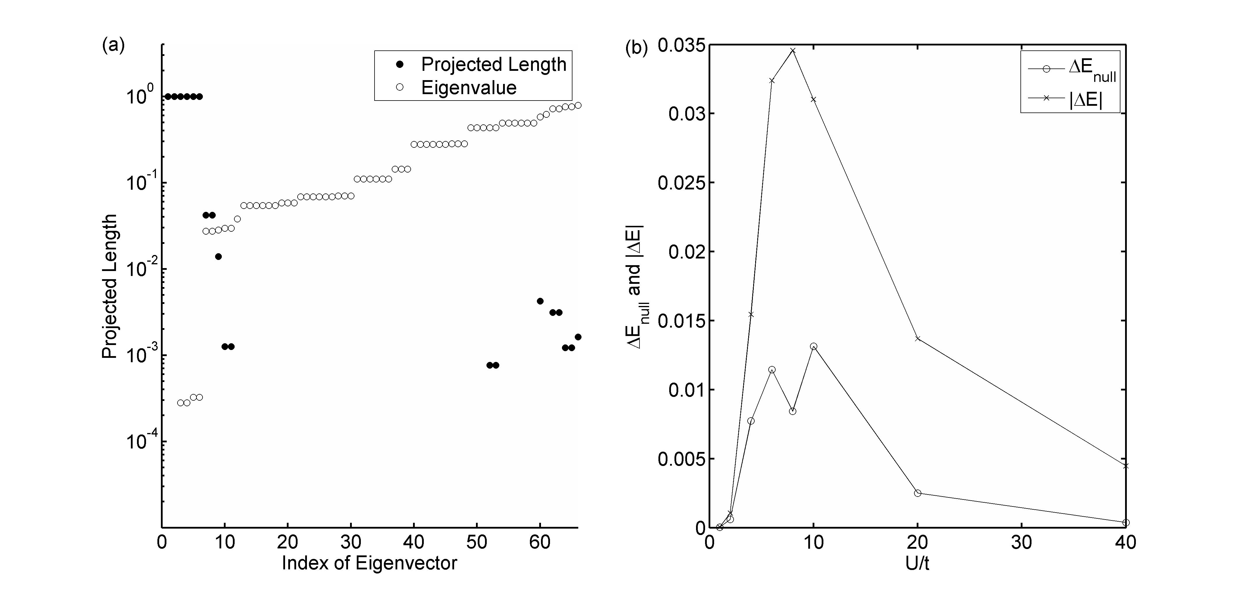
Figure 1: (a) The projection length (filled circle) of the eigenvector of $D_{exact}$ in the null space of $D_{var}$ together with the corresponding eigenvalues (open circle). The eigenvalues of $D_{exact}$ are sorted in ascending order. The results are for 1D Hubbard model with $U/t=10$. The null space of $D_{var}$ has overlap with 10 low-lying and 8 high-lying eigenvectors of $D_{exact}$. (b) The contribution of the $D_{var}$ null space to the deviation of variational total energy for 1D Hubbard model with $U/t=1,2,4,6,8,10,20,40$, respectively. The contribution is largely correlated with the deviation of variational total energy.

$G_{var}$ has five more null eigenvalues than $G_{exact}$. As discussed in previous section, if $G_{var}$ is $N$-representable, the eight corresponding null eigenoperators must form the complete basis set of a Lie algebra. That is, For two null eigenoperators $g_{m}$ and $g_{n}$ in $\mathfrak{n}_{G}$, $\left[g_{m},g_{n}\right]|\Psi\rangle=0$.

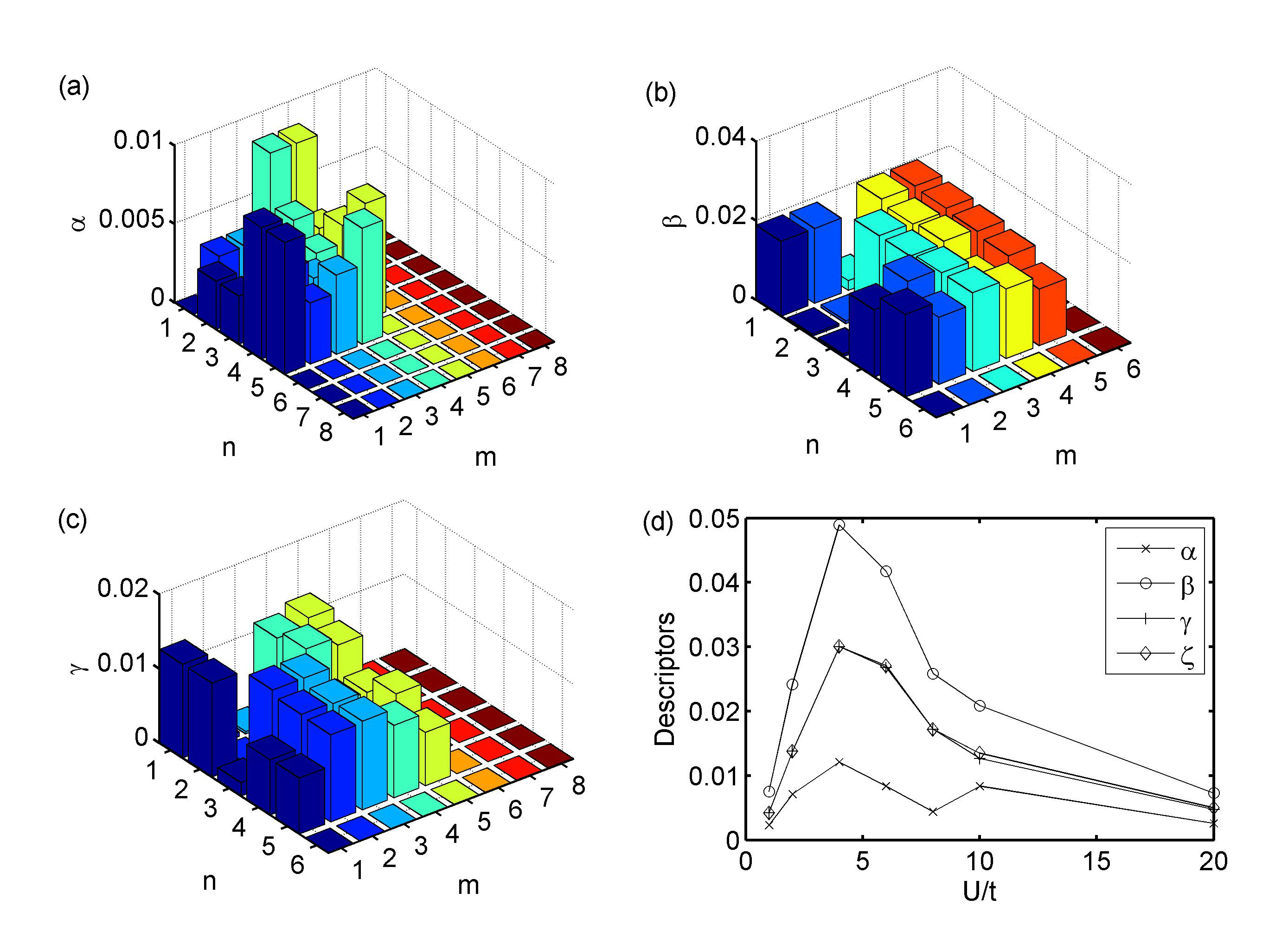
Figure 2: The constraint test on the variational RDMs of Hubbard model. (a) The length of vector $\left[g_{m},g_{n}\right]|\Psi\rangle$ with $m,n=1,2,\cdots,8$ corresponding to the eight null eigenoperators of $G_{var}$. (b) The length of vector $\left[d_{m},q_{n}\right]|\Psi\rangle$ with $m,n=1,2,\cdots,6$ corresponding to the six null eigenoperators of $D_{var}$ and $Q_{var}$. (c) The length of vector $\left[g_{m},d_{n}\right]|\Psi\rangle$ with $m=1,2,\cdots,8$ and $n=1,2,\cdots,6$ corresponding to the eight null eigenoperators of $G_{var}$ and six for $Q_{var}$. The maximal lengths in (a), (b) and (c) are, respectively, about 0.0078, 0.021 and 0.015. Apparently, many of the commutators are not null operators of the state $|\Psi\rangle$, therefore $D_{var}$, $G_{var}$ and $Q_{var}$ are not $N$-representable. (d) The constraint violation descriptors $I_{\alpha}$, $I_{\beta}$, $I_{\gamma}$ and $I_{\zeta}$ for the Hubbard model with $U/t=1,2,4,6,8,10,20,40$. The maximum of four descripters is around $U/t=4$. While, the maximal deviation of variational energy is at $U/t=8$ (see Fig. 1(b)). Therefore, the structure deviation of the variational 2-RDM is not correlated with the error of the total energy.

We use Eq.(7a) and (7b) to verify whether the variational 2-RDMs are $N$-representable. Fig. 2(a) shows $\alpha_{mn}$ for the null eigenoperators of $G_{var}$. There are multiple non-vanishing values. Therefore, the null eigenoperators of $G_{var}$ do not form a closed subalgebra, and $G_{var}$ is not $N$-representable.

$Q_{var}$ has five more null eigenvalues than $Q_{exact}$. If $Q_{var}$ and $D_{var}$ are $N$-representable, the commutator of their null eigenoperators must be a null eigenoperator in $\mathfrak{n}_{G}$. Fig.2(b) shows the the $\beta_{mn}$ evaluated from the null eigenoperators of $Q_{var}$ and $D_{var}$. The values are in the order of $10^{-2}$ and, clearly, violate the $N$-representability constraint. The constraint violation is aslo prominent for the commutors of the null eigenoperators for $G_{var}$ and $D_{var}$ (Fig. 2(c)).

The numerical results for Hubbard model show that the constraints impose strong restrictions on the null spaces of 2-RDMs. To quantify the degree of constraint violation by variational 2-RDMs, we introduce a descriptor $I_{\alpha}$ defined as the maximum value of $\alpha_{mn}$ from the null eigenoperators of $G$. A large value of descriptor suggests strong violation. Similarly, we may define descriptors $I_{\beta}$, $I_{\gamma}$ and $I_{\zeta}$ for the maximum value of $\beta_{mn}$, $\gamma_{mn}$ and $\zeta_{mn}$, respectively. The four descriptors of the Hubbard model with $U/t=10$ are shown in Table 1.

$N$-representability requires the constraints on the null spaces of 2-RDMs:

$$I_{\alpha}=I_{\beta}=I_{\gamma}=I_{\zeta}=0.$$ (22)

Fig. 2(d) shows the trend of constraint violation by variational 2-RDMs as $U/t$ of Hubbard model varying. In general, we can see to $I_{\beta}>I_{\gamma}\approx I_{\zeta}>I_{\alpha}$. The maximum of these descriptors is around $U/t=4$, which is different from that for the variational energy deviation (around $U/t=8$ as shown in Fig. 1(b)).

LiH and random-matrix Hamiltonians

The violation of the null space constraint seems general for variational 2-RDM. For the diatomic molecule LiH in its equilibrium configuration, the variational method can provide the very accurate estimation of ground state energy with $\Delta E\sim 2.0\times 10^{-8}$ (see Table A2). However, the dimensions of the null spaces of variational 2-RDMs are very different from that of the exact 2-RDMs (see Table A2 and Table 1), which indicates the disparity in the Lie algebra structure of their null eigenoperators. The descriptor $I_{\beta}=0.30\times 10^{-3}$, which is about 5 order of magnitude larger than the numerical accuracy of our variational calculation.

In order to have a rough idea how often the variational 2-RDM method may predict erroneous null spaces of RDMs, we have applied the method to five Hamiltonians with randomly generated numbers in spatial degree of freedom. The erroneous null spaces have been found in all five cases. The results for two of them are shown in Table A3 and A4. As summarized in Table 1, the exact RDMs of the ground states have 3 null eigenoperators corresponding to 3 spin operators. While, the variational RDMs have more null eigenoperators. The four descriptors are not vanishing for these RDMs.

From Table 1, we can have two interesting observations. In contrast to Hubbard model, a strongly correlated system, the $\Delta E_{null}/\left|\Delta E\right|$ (~5%) of the random systems is quite small, and the null space of $D_{var}$ has very small contribution to the ground state energy deviation $\Delta E$. We belive, $\Delta E_{null}/\left|\Delta E\right|$ (-67%) for LiH is problematic because both $\left|\Delta E_{null}\right|$ and $\left|\Delta E\right|$ are on the of $10^{-8}$ and close to numerical accuracy $1.0\times 10^{-9}$. For variation RDMs, the descriptor $I_{\beta}$ , $I_{\gamma}$ and $I_{\zeta}$ are usually larger than $I_{\alpha}$. This may suggest that the constraint on the null spaces of $D$ and $Q$ matrices is stronger than that on $G$ matrix. Apparently, more numerical studies are needed in future in order to tell whether the observations are general.

Inequality Constraints on the Whole Eigenspaces of RDMs

The constraints presented so far are only applied to the null spaces of RDMs. To derive the constraints covering the whole eigenspaces of RDMs, we first use commutation relation of two operators to have a vector equation:

$$p_{1}p_{2}|\Psi\rangle-p_{2}p_{1}|\Psi\rangle=p_{3}|\Psi\rangle,$$

here $p_{1}$, $p_{2}$ and $p_{3}$ are three pair operators in $\mathfrak{h}$ satisfying $p_{3}=\left[p_{1},p_{2}\right]$. Using triangle inequality, we have

$$\left|p_{3}|\Psi\rangle\right|\leq\left|p_{1}p_{2}|\Psi\rangle\right|+\left|p_{2}p_{1}|\Psi\rangle\right|$$ (23)

with $\left|p_{1}p_{2}|\Psi\rangle\right|^{2}=\langle\Psi|p_{2}^{\dagger}p_{1}^{\dagger}p_{1}p_{2}|\Psi\rangle$, $\left|p_{2}p_{1}|\Psi\rangle\right|^{2}=\langle\Psi|p_{1}^{\dagger}p_{2}^{\dagger}p_{2}p_{1}|\Psi\rangle$ and $\left|p_{3}|\Psi\rangle\right|^{2}=\langle\Psi|p_{3}^{\dagger}p_{3}|\Psi\rangle$. To find the upper bound of $\langle\Psi|p_{2}^{\dagger}p_{1}^{\dagger}p_{1}p_{2}|\Psi\rangle$, let $|\phi\rangle=\frac{p_{2}|\Psi\rangle}{\left|p_{2}|\Psi\rangle\right|}$ and insert it into the inner product. W have

$$\langle\Psi|p_{2}^{\dagger}p_{1}^{\dagger}p_{1}p_{2}|\Psi\rangle =\langle\Psi|p_{2}^{\dagger}|\phi\rangle\langle\phi|p_{1}^{\dagger}p_{1}|\phi\rangle\langle\phi|p_{2}|\Psi\rangle$$

$$=\langle\phi|p_{1}^{\dagger}p_{1}|\phi\rangle\langle\Psi|p_{2}^{\dagger}|\phi\rangle\langle\phi|p_{2}|\Psi\rangle$$

$$=\langle\phi|p_{1}^{\dagger}p_{1}|\phi\rangle\langle\Psi|p_{2}^{\dagger}p_{2}|\Psi\rangle$$

$$\leq c_{1}\langle\Psi|p_{2}^{\dagger}p_{2}|\Psi\rangle$$ (24)

here $\langle\phi|p_{1}^{\dagger}p_{1}|\phi\rangle$ is upper bounded by $c_{1}$. Similarly, we can have

$$\langle\Psi|p_{1}^{\dagger}p_{2}^{\dagger}p_{2}p_{1}|\Psi\rangle\leq c_{2}\langle\Psi|p_{1}^{\dagger}p_{1}|\Psi\rangle$$ (25)

with $|\varphi\rangle=\frac{p_{1}|\Psi\rangle}{\left|p_{1}|\Psi\rangle\right|}$ and $\langle\varphi|p_{2}^{\dagger}p_{2}|\varphi\rangle$ is upper bounded by $c_{2}$. From Eq.(23), (24) and (25), we have

$$\left|p_{3}|\Psi\rangle\right|\leq c_{1}^{\frac{1}{2}}\left|p_{2}|\Psi\rangle\right|+c_{2}^{\frac{1}{2}}\left|p_{1}|\Psi\rangle\right|$$ (26)

Substituting $p_{1}$ and $p_{2}$ in Eq.(26) by two eigenoperators, and using the commutation relations: Eq.(5a) to (6d), the constraints on the eigenspaces of 2-RMDs are given by

$$\alpha_{mn}\leq\left(\overline{\lambda}_{N}^{G}\right)^{\frac{1}{2}}\left[\left(\lambda_{m}^{G}\right)^{\frac{1}{2}}+\left(\lambda_{n}^{G}\right)^{\frac{1}{2}}\right],$$ (27a)

$$\beta_{mn}\leq\left(\overline{\lambda}_{N-2}^{Q}\right)^{\frac{1}{2}}\left(\lambda_{m}^{D}\right)^{\frac{1}{2}}+\left(\overline{\lambda}_{N+2}^{D}\right)^{\frac{1}{2}}\left(\lambda_{n}^{Q}\right)^{\frac{1}{2}},$$ (27b)

$$\gamma_{mn}\leq\left(\overline{\lambda}_{N}^{D}\right)^{\frac{1}{2}}\left(\lambda_{m}^{G}\right)^{\frac{1}{2}}+\left(\overline{\lambda}_{N-2}^{G}\right)^{\frac{1}{2}}\left(\lambda_{n}^{D}\right)^{\frac{1}{2}},$$ (27c)

and

$$\zeta_{mn}\leq\left(\overline{\lambda}_{N}^{Q}\right)^{\frac{1}{2}}\left(\lambda_{m}^{G}\right)^{\frac{1}{2}}+\left(\overline{\lambda}_{N+2}^{G}\right)^{\frac{1}{2}}\left(\lambda_{n}^{Q}\right)^{\frac{1}{2}}.$$ (27d)

Here $\overline{\lambda}_{N}^{D}$, $\overline{\lambda}_{N}^{G}$ and $\overline{\lambda}_{N}^{Q}$ are, respectively, the upper bounds for the eigenvalues of $G,$$D$ and $Q$ matrices for a $N$-electron state. We refer the four constraints as $\alpha,$ $\beta$, $\gamma$ and $\zeta$ conditions. They are necessary $N$-representability conditions. The constraints on the null spaces, Eq.(22), are special cases of above inequalities where the eigenvalues on the right side vanish. From Eq.(26), we can see that these constraints are of geometric nature.

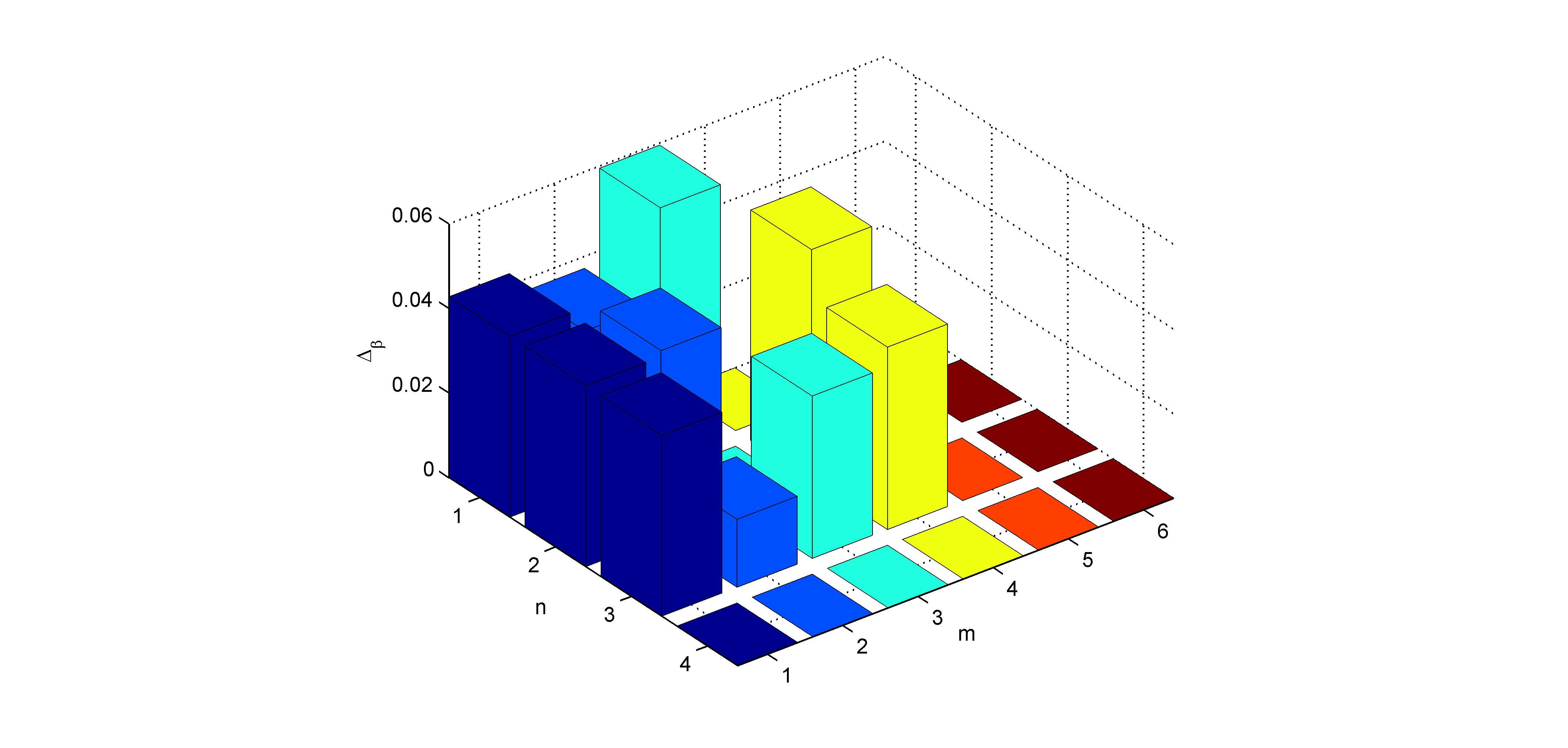
Figure 3: An example for violation of the inquality constraints. The system is a random-matrix Hamiltonians (Table A3). $\Delta_{\beta}$ is an descriptor of constraint violation (see the definition in text). $\Delta_{\beta}>0$ indicates constraint violation. $m$ and $n$ are the indices of the eigenvalues of $D$ and $Q$, respectively. The three dark blue bars indicate the violation of the equality constraint Eq.(22) by the variational 2-RDMs. The other bars show the explicit violation of inequality constraints.

Fig. 3 show an example where a variationl 2-RDM violates the inequality constants Eq.(27b). The system is a random-matrix Hamiltonians (Table A3). The descriptor of constraint violation is $\Delta_{\beta}\left(m,n\right)=\beta_{mn}-\left[\frac{L-N+2}{2}\right]^{\frac{1}{2}}\left(\lambda_{m}^{D}\right)^{\frac{1}{2}}-\left[\frac{N+2}{2}\right]^{\frac{1}{2}}\left(\lambda_{n}^{Q}\right)^{\frac{1}{2}}.$ $\Delta_{\beta}>0$ indicates constraint violation. we have set $\overline{\lambda}_{N+2}^{D}=\left[\frac{N+2}{2}\right]$ and $\overline{\lambda}_{N-2}^{Q}=\left[\frac{L-N+2}{2}\right]$ , respectively, the universal upper bounds for the eigenvalues of $D$ and $Q$ matrices.(Sasaki, 1965) $m$ and $n$ are the indices of the eigenvalues of $D$ and $Q$, respectively. As shown in Table A3, $D_{var}$ has one null eigenvalue corresponding to $m=1$, and $Q_{var}$ has three corresponding to $n=1,2,3$. Therefore, the three dark blue bars in Fig.3 indicate the violation of the equality constraint Eq.(22). The other bars show the explicit violation of inequality constraints.

Discussion and Conclusion

Even though the derivation of geometric constraints is started with a wave function in $N$-electron Fock space, these constraints are actually ensemble $N$-representability conditions because any mixed state can be mapped onto a pure state in a larger space (known as purification of mixed state in quantum information).(Kleinmann et al., 2006)

The null eigenoperators of 2-RDMs carry the information about the conserved observables of the underlying many-electron state. Eq.(22) imposes restrictions on the null eigenspace of 2-RDMs to ensure the commmutative compatibility of these observables. More ganerally, if $|\Psi\rangle$ is an eigenstate of a two-electron operator, $H=\sum_{ij,kl}K_{ij,kl}a_{i}^{\dagger}a_{j}^{\dagger}a_{l}a_{k}$, then we can generate a set of two-electron null operators by $\left\{\left[\mathfrak{n}_{G},H\right],\left[\mathfrak{n}_{G},\left[\mathfrak{n}_{G},H\right]\right],\cdots\right\}$, which provides additional constraints on the 2-RDMs. Prediction of fractional charges and fractiona spins is an indication of insufficient constraint on the conserved observables in various RDM-based electronic structure methods.

The results shown in Fig. 2(d) and for LiH suggests that, for variational 2-RDM method, a smaller error in variational energy is not necessarily implying a smaller structural deviation of 2-RDM. The structural deviation may lead to erroneous prediction of important electronic structure properties such as the order parameters in condensed state physics.

Explicit violation of inequality constraints by variation 2-RDMs is not found for the Hubbard model and LiH, most likely, due to the insufficiency of the universal upper bounds used in our tests. The sharp upper bounds proposed by Van Neck, Johnson and their coworkers(Neck and Ayers, 2007; Johnson et al., 2013) may be useful to ehnace the inequality constraints.

Substituting an eigenoperator of 1-RDM and an eigenoperator of 2-RDM in Eq.(26), we can also obtain more constraints on the eigenspace of 1-RDM and 2-RDM. Eq.(26) is general for operators defined on any Hilbert space. Therefore, the approach presented here is applicable to characterize not only $N$-representability of fermions but also that of bosons and quantum marginal problem in general.

In this work, we derive a set of necessary $N$-representability conditions on 2-RDMs based on the basic geometric property of Hilbert and the commutation relations of operators. We show that the algebra properties of the eigenoperators of 2-RDMs lead to equality constraints on the null spaces of 2-RDMs. Using triangle inequality, a further analysis results in a set of inequalities expanding the constraints to the whole eigenspace of 2-RDMs. Numerical tests show that, compared to the available positive semidefinite conditions on 2-RDMs, these conditions impose more stringent constraint on the structure of 2-RDMs.

Implementing the geometric constraints in ground-state-energy optimization will not be straightforward due to their nonlinear nature. Incorporation into SDP may be carried out in a self-consistent manor, in which these conditions provide correction to varitional RDMs and new approximated constraints for the next round SDP optimization. However, this may lead to significant increase of computational cost. Another interesting direction to explore is their application in hybrid quantum-classical computing.(Rubin et al., 2018; Smart and Mazziotti, 2019) Recent progresses show that $N$-representability conditions can be utilized to mitigate quantum error in electronic structure simulations, and to reduce the number of required quantum measurements by one order.

References

Appendix

Derivation of the commutation relations for 2-RDM eigenoperators

(a) For $g_{m}$ and $g_{n}$, two eigenoperators of $G$ matrix,

$$\left[g_{m},g_{n}\right] =\sum_{i,j=1}^{L}\sum_{k,l=1}^{L}\left[v_{ij}^{m}a_{j}^{\dagger}a_{i},v_{kl}^{n}a_{l}^{\dagger}a_{k}\right]$$

$$=\sum_{i,j=1}^{L}\sum_{k,l=1}^{L}v_{ij}^{m}v_{kl}^{n}\left[a_{j}^{\dagger}a_{i},a_{l}^{\dagger}a_{k}\right]$$

$$=\sum_{i,j=1}^{L}\sum_{k,l=1}^{L}v_{ij}^{m}v_{kl}^{n}\left(a_{j}^{\dagger}a_{k}\delta_{il}-a_{l}^{\dagger}a_{i}\delta_{jk}\right)$$

$$=\sum_{j,k,l=1}^{L}v_{lj}^{m}v_{kl}^{n}a_{j}^{\dagger}a_{k}-\sum_{i,k,l=1}^{L}v_{ik}^{m}v_{kl}^{n}a_{l}^{\dagger}a_{i}$$

$$=\sum_{i,j=1}^{L}\left[\sum_{k=1}^{L}\left(v_{kj}^{m}v_{ik}^{n}-v_{ik}^{m}v_{kj}^{n}\right)\right]a_{j}^{\dagger}a_{i}$$

$$=\sum_{i,j=1}^{L}\overline{v}_{ij}^{mn}a_{j}^{\dagger}a_{i},$$ (A1a)

here

$$\overline{v}_{ij}^{mn}=\sum_{k=1}^{L}\left(v_{kj}^{m}v_{ik}^{n}-v_{ik}^{m}v_{kj}^{n}\right).$$ (A1b)

Now expanding $\overline{\boldsymbol{v}}^{mn}$ in the basis set $\left\{v_{ij}^{m^{\prime}},m^{\prime}=1,2,\cdots,L^{2}\right\}$, we have

$$\left[g_{m},g_{n}\right] =\sum_{m^{\prime}=1}^{L^{2}}\sum_{i,j=1}^{L}\left(\sum_{k,l=1}^{L}\overline{v}_{kl}^{mn}v_{kl}^{m^{\prime}*}\right)v_{ij}^{m^{\prime}}a_{j}^{\dagger}a_{i}$$

$$=\sum_{m^{\prime}=1}^{L^{2}}\Gamma_{mn}^{m^{\prime}}g_{m^{\prime}},$$ (A1c)

here

$$\Gamma_{mn}^{m^{\prime}} =\sum_{i,j=1}^{L}\overline{v}_{ij}^{mn}v_{ij}^{m^{\prime}*}$$

$$=\sum_{i,j,k=1}^{L}\left(v_{kj}^{m}v_{ik}^{n}-v_{ik}^{m}v_{kj}^{n}\right)v_{ij}^{m^{\prime}*}$$ (A1d)

(b) For $g_{m}$ and $d_{n}$, two eigenoperators of $G$ and $D$ matrix, respectively,

$$\left[g_{m},d_{n}\right] =\sum_{i,j=1}^{L}\sum_{k,l=1}^{L}\left[v_{ij}^{m}a_{j}^{\dagger}a_{i},u_{kl}^{n}a_{l}a_{k}\right]$$

$$=\sum_{i,j=1}^{L}\sum_{k,l=1}^{L}v_{ij}^{m}u_{kl}^{n}\left[a_{j}^{\dagger}a_{i},a_{l}a_{k}\right]$$

$$=\sum_{i,j=1}^{L}\sum_{k,l=1}^{L}v_{ij}^{m}u_{kl}^{n}\left(a_{k}a_{i}\delta_{jl}-a_{l}a_{i}\delta_{jk}\right)$$

$$=\sum_{i,k,l=1}^{L}\left(v_{il}^{m}u_{kl}^{n}a_{k}a_{i}-v_{ik}^{m}u_{kl}^{n}a_{l}a_{i}\right)$$

$$=\sum_{i,j=1}^{L}\left[\sum_{k=1}^{L}\left(v_{ik}^{m}u_{jk}^{n}-v_{ik}^{m}u_{kj}^{n}\right)\right]a_{j}a_{i}$$

$$=\sum_{i,j=1}^{L}\overline{u}_{ij}^{mn}a_{j}a_{i},$$ (A2a)

here

$$\overline{u}_{ij}^{mn} =\sum_{k=1}^{L}\left(v_{ik}^{m}u_{jk}^{n}-v_{ik}^{m}u_{kj}^{n}\right)$$

$$=-2\sum_{k=1}^{L}v_{ik}^{m}u_{kj}^{n}.$$ (A2b)

Here, we have used the fact, $$u_{jk}^{n}=-u_{kj}^{n} \overline{\boldsymbol{u}}^{mn} \left\{u_{ij}^{m^{\prime}},m^{\prime}=1,2,\cdots,\frac{L\left(L-1\right)}{2}\right\}$$. Now expanding in the basis set , we have

$$\left[g_{m},d_{n}\right] =\sum_{m^{\prime}=1}^{\frac{L\left(L-1\right)}{2}}\sum_{i,j=1}^{L}\left(\sum_{k,l=1}^{L}\overline{u}_{kl}^{mn}u_{kl}^{m^{\prime}*}\right)u_{ij}^{m^{\prime}}a_{j}a_{i}$$

$$=\sum_{m^{\prime}=1}^{\frac{L\left(L-1\right)}{2}}\Delta_{mn}^{m^{\prime}}d_{m^{\prime}},$$ (A2c)

here

$$\Delta_{mn}^{m^{\prime}} =\sum_{i,j=1}^{L}\overline{u}_{ij}^{mn}u_{ij}^{m^{\prime}*}$$

$$=-2\sum_{i,j,k=1}^{L}v_{ik}^{m}u_{kj}^{n}u_{ij}^{m^{\prime}*}$$ (A2d)

(c) For $g_{m}$ and $q_{n}$, two eigenoperators of $G$ and $Q$ matrix, respectively,

$$\left[g_{m},q_{n}\right] =\sum_{i,j=1}^{L}\sum_{k,l=1}^{L}\left[v_{ij}^{m}a_{j}^{\dagger}a_{i},w_{kl}^{n}a_{l}^{\dagger}a_{k}^{\dagger}\right]$$

$$=\sum_{i,j=1}^{L}\sum_{k,l=1}^{L}v_{ij}^{m}w_{kl}^{n}\left[a_{j}^{\dagger}a_{i},a_{l}^{\dagger}a_{k}^{\dagger}\right]$$

$$=\sum_{i,j=1}^{L}\sum_{k,l=1}^{L}v_{ij}^{m}w_{kl}^{n}\left(a_{j}^{\dagger}a_{k}^{\dagger}\delta_{il}-a_{j}^{\dagger}a_{l}^{\dagger}\delta_{ik}\right)$$

$$=\sum_{j,k,l=1}^{L}\left(v_{lj}^{m}w_{kl}^{n}a_{j}^{\dagger}a_{k}^{\dagger}-v_{kj}^{m}w_{kl}^{n}a_{j}^{\dagger}a_{l}^{\dagger}\right)$$

$$=\sum_{i,j=1}^{L}\left[\sum_{k=1}^{L}\left(v_{kj}^{m}w_{ik}^{n}-v_{kj}^{m}w_{ki}^{n}\right)\right]a_{j}^{\dagger}a_{i}^{\dagger}$$

$$=\sum_{i,j=1}^{L}\overline{w}_{ij}^{mn}a_{j}^{\dagger}a_{i}^{\dagger},$$ (A3a)

here

$$\overline{w}_{ij}^{mn} =\sum_{k=1}^{L}\left(v_{kj}^{m}w_{ik}^{n}-v_{kj}^{m}w_{ki}^{n}\right)$$

$$=2\sum_{k=1}^{L}w_{ik}^{n}v_{kj}^{m}.$$ (A3b)

Here, we have used the fact, $$w_{jk}^{n}=-w_{kj}^{n} \overline{\boldsymbol{w}}^{mn} \left\{w_{ij}^{m^{\prime}},m^{\prime}=1,2,\cdots,\frac{L\left(L-1\right)}{2}\right\}$$. Now expanding in the basis set , we have

$$\left[g_{m},q_{n}\right] =\sum_{m^{\prime}=1}^{\frac{L\left(L-1\right)}{2}}\sum_{i,j=1}^{L}\left(\sum_{k,l=1}^{L}\overline{w}_{kl}^{mn}w_{kl}^{m^{\prime}*}\right)w_{ij}^{m^{\prime}}a_{j}^{\dagger}a_{i}^{\dagger}$$

$$=\sum_{m^{\prime}=1}^{\frac{L\left(L-1\right)}{2}}\Omega_{mn}^{m^{\prime}}q_{m^{\prime}},$$ (A3c)

here

$$\Omega_{mn}^{m^{\prime}} =\sum_{i,j=1}^{L}\overline{w}_{ij}^{mn}w_{ij}^{m^{\prime}*}$$

$$=2\sum_{i,j,k=1}^{L}w_{ik}^{n}v_{kj}^{m}w_{ij}^{m^{\prime}*}$$ (A3d)

(d) For $q_{m}$ and $d_{n}$, two eigenoperators of $Q$ and $D$ matrix, respectively,

$$\left[q_{m},d_{n}\right] =\sum_{i,j=1}^{L}\sum_{k,l=1}^{L}\left[w_{ij}^{m}a_{j}^{\dagger}a_{i}^{\dagger},u_{kl}^{n}a_{l}a_{k}\right]$$

$$=\sum_{i,j=1}^{L}\sum_{k,l=1}^{L}w_{ij}^{m}u_{kl}^{n}\left[a_{j}^{\dagger}a_{i}^{\dagger},a_{l}a_{k}\right]$$

$$=\sum_{i,j=1}^{L}\sum_{k,l=1}^{L}w_{ij}^{m}u_{kl}^{n}\left(a_{j}^{\dagger}a_{k}\delta_{il}-a_{j}^{\dagger}a_{l}\delta_{ik}+a_{k}a_{i}^{\dagger}\delta_{jl}-a_{l}a_{i}^{\dagger}\delta_{jk}\right)$$

$$=\sum_{i,j=1}^{L}\sum_{k,l=1}^{L}w_{ij}^{m}u_{kl}^{n}\left(a_{j}^{\dagger}a_{k}\delta_{il}-a_{j}^{\dagger}a_{l}\delta_{ik}-a_{i}^{\dagger}a_{k}\delta_{jl}+a_{i}^{\dagger}a_{l}\delta_{jk}+\delta_{ik}\delta_{jl}-\delta_{il}\delta_{jk}\right)$$

$$=\sum_{j,k,l=1}^{L}\left(w_{lj}^{m}u_{kl}^{n}a_{j}^{\dagger}a_{k}-w_{kj}^{m}u_{kl}^{n}a_{j}^{\dagger}a_{l}\right)+\sum_{i,k,l=1}^{L}\left(-w_{il}^{m}u_{kl}^{n}a_{i}^{\dagger}a_{k}+w_{ik}^{m}u_{kl}^{n}a_{i}^{\dagger}a_{l}\right)+\sum_{k,l=1}^{L}\left(w_{kl}^{m}u_{kl}^{n}-w_{lk}^{m}u_{kl}^{n}\right)$$

$$=\sum_{i,j=1}^{L}\left[\sum_{k=1}^{L}\left(w_{kj}^{m}u_{ik}^{n}-w_{lj}^{m}u_{ki}^{n}-w_{jk}^{m}u_{ik}^{n}+w_{jk}^{m}u_{ki}^{n}\right)\right]a_{j}^{\dagger}a_{i}+\sum_{k,l=1}^{L}\left(w_{kl}^{m}u_{kl}^{n}-w_{lk}^{m}u_{kl}^{n}\right)$$

$$=\sum_{i,j=1}^{L}\left[\sum_{k=1}^{L}\left(w_{kj}^{m}u_{ik}^{n}-w_{kj}^{m}u_{ki}^{n}-w_{jk}^{m}u_{ik}^{n}+w_{jk}^{m}u_{ki}^{n}\right)+\frac{1}{N}\sum_{k,l=1}^{L}\left(w_{kl}^{m}u_{kl}^{n}-w_{lk}^{m}u_{kl}^{n}\right)\delta_{ij}\right]a_{j}^{\dagger}a_{i}$$

$$=\sum_{i,j=1}^{L}\overline{v}_{ij}^{mn}a_{j}^{\dagger}a_{i},$$ (A4a)

here, we have restricted ourselves in $$N$$-electron Fock space, and

$$\overline{v}_{ij}^{mn} =\sum_{k=1}^{L}\left(w_{kj}^{m}u_{ik}^{n}-w_{kj}^{m}u_{ki}^{n}-w_{jk}^{m}u_{ik}^{n}+w_{jk}^{m}u_{ki}^{n}\right)+\frac{1}{N}\sum_{k,l=1}^{L}\left(w_{kl}^{m}u_{kl}^{n}-w_{lk}^{m}u_{kl}^{n}\right)$$

$$=4\left(\sum_{k=1}^{L}u_{ik}^{n}w_{kj}^{m}-\frac{1}{2N}\delta_{ij}\sum_{k,l=1}^{L}u_{lk}^{n}w_{kl}^{m}\right)$$ (A4b)

Here, we have used the fact, $$u_{jk}^{n}=-u_{kj}^{n} w_{jk}^{n}=-w_{kj}^{n} \overline{\boldsymbol{v}}^{mn} \left\{v_{ij}^{m^{\prime}},m^{\prime}=1,2,\cdots,L^{2}\right\}$$ and . Now expanding in the basis set , we have

$$\left[q_{m},d_{n}\right] =4\sum_{m^{\prime}=1}^{L^{2}}\sum_{i,j=1}^{L}\left(\sum_{k=1}^{L}u_{ik}^{n}w_{kj}^{m}-\frac{1}{2N}\delta_{ij}\sum_{k,l=1}^{L}u_{lk}^{n}w_{kl}^{m}\right)v_{ij}^{m^{\prime}}a_{j}^{\dagger}a_{i}$$

$$=\sum_{m^{\prime}=1}^{L^{2}}\Theta_{mn}^{m^{\prime}}g_{m^{\prime}},$$ (A4c)

here

$$\Omega_{mn}^{m^{\prime}} =\sum_{i,j=1}^{L}\overline{v}_{ij}^{mn}v_{ij}^{m^{\prime}*}$$

$$=4\sum_{i,j,k=1}^{L}\left(u_{ik}^{n}w_{kj}^{m}-\frac{1}{2N}\delta_{ij}\sum_{l=1}^{L}u_{lk}^{n}w_{kl}^{m}\right)v_{ij}^{m^{\prime}*}$$

$$=4\sum_{i,j,k=1}^{L}\left(u_{ik}^{n}w_{kj}^{m}v_{ij}^{m^{\prime}*}-\frac{1}{2N}u_{ij}^{n}w_{ji}^{m}v_{kk}^{m^{\prime}*}\right)$$ (A4d)

Table A1: The ten lowest eigenvalues of the variational and exact RDMs for a 6-site half-filled 1D Hubbard model with $t=1$ and $U=10$. The ground state energies obtained by the two methods are $E_{exact}=-1.664362733287$ and $E_{var}=-1.695384327725$, respectively. The energy deviation $\Delta E=-0.031021594438$. These energies are consistent with the previous studies on this model.(Nakata et al., 2008)

	D matrix				G matrix				Q matrix
n	Variational		Exact		Variational		Exact		Variational		Exact
1	-0.	000000000001	-0.	000000000000	-0.	000000000000	-0.	000000000000	-0.	000000000001	0.	000000000000
2	-0.	000000000001	0.	000013764099	-0.	000000000000	-0.	000000000000	-0.	000000000001	0.	000013764099
3	-0.	000000000001	0.	000558839696	-0.	000000000000	0.	000000000000	-0.	000000000001	0.	000558839696
4	-0.	000000000001	0.	000558839696	-0.	000000000000	0.	000006882049	-0.	000000000001	0.	000558839696
5	-0.	000000000001	0.	000649120541	-0.	000000000000	0.	000279419848	-0.	000000000001	0.	000649120541
6	-0.	000000000000	0.	000649120541	0.	000000000000	0.	000279419848	-0.	000000000000	0.	000649120541
7	0.	052344794130	0.	054771204301	0.	000000000000	0.	000324560271	0.	052344794122	0.	054771204301
8	0.	052344794130	0.	054771204301	0.	000000000000	0.	000324560271	0.	052344794122	0.	054771204301
9	0.	053848732617	0.	056628436116	0.	019332198318	0.	026343666870	0.	053848732627	0.	056628436116
10	0.	054329721649	0.	059289055684	0.	025473863823	0.	027040912995	0.	054329721653	0.	059289055684

Table A2: The five lowest eigenvalues of the variational and exact RDMs for diatomic molecule LiH. The ground state energies obtained by the two methods are $E_{exact}=-8.967211312701\,(E_{h})$ and $E_{var}=-8.967211329766\,(E_{h})$, respectively. The energy deviation $\Delta E=-1.707\times 10^{-8}\,(E_{h})$. These energies are consistent with the previous studies on this system.(Zhao et al., 2004; Nakata et al., 2008)

	D matrix				G matrix				Q matrix
n	Variational		Exact		Variational		Exact		Variational		Exact
1	0.	000000000671	0.	000000001019	-0.	000000000000	-0.	000000000000	0.	000000000137	0.	000000014488073
2	0.	000000000920	0.	000000011154	0.	000000000000	0.	000000000000	0.	000001131230	0.	000001027814592
3	0.	000000004001	0.	000000011154	-0.	000000000000	-0.	000000000000	0.	000001245966	0.	000001179234760
4	0.	000000004001	0.	000000011154	-0.	000000000000	-0.	000000000000	0.	000001245966	0.	000001179234760
5	0.	000000007047	0.	000000011154	-0.	000000000863	-0.	000000000000	0.	000001245966	0.	000001179234760

Table A3: The eight lowest eigenvalues of the variational and exact RDMs for random hamiltonian 1. The hamiltonian matrix elements in the spatial degree of freedom are randomly generated with a uniform distribution in $[0,1)$.The ground state energies obtained by the two methods are $E_{exact}=-5.474591092179$ and $E_{var}=-5.601757205138$, respectively. The energy deviation $\Delta E=-0.127166112960$.

	D matrix				G matrix				Q matrix
n	Variational		Exact		Variational		Exact		Variational		Exact
1	0.	000000000000	0.	000143928633	-0.	000000000000	-0.	000000000000	0.	000000000017	0.	001790119018
2	0.	000613559566	0.	001929013145	-0.	000000000000	-0.	000000000000	0.	000000000017	0.	002205303031
3	0.	000613559566	0.	001929013145	-0.	000000000000	0.	000000000000	0.	000000000017	0.	002205303031
4	0.	000613559566	0.	001929013145	0.	000000000006	0.	000653753069	0.	005038116249	0.	002205303031
5	0.	005911622327	0.	002005631157	0.	000000000006	0.	000653753069	0.	007038945113	0.	004683583778
6	0.	005911622327	0.	003709814514	0.	000000000006	0.	000653753069	0.	007038945113	0.	004770757563
7	0.	005911622327	0.	003709814514	0.	000000000006	0.	000821845808	0.	007038945113	0.	004770757563
8	0.	006553183666	0.	003709814514	0.	001077905210	0.	000908689956	0.	017400000968	0.	004770757563

Table A4: The eight lowest eigenvalues of the variational and exact RDMs for random Hamiltonian 2. The Hamiltonian matrix elements in the spatial degree of freedom are randomly generated with a uniform distribution in $[0,1)$.The ground state energies obtained by the two methods are $E_{exact}=-9.559169540991$ and $E_{var}=-9.571940687877$, respectively. The energy deviation $\Delta E=-0.012771146886$.

	D matrix				G matrix				Q matrix
n	Variational		Exact		Variational		Exact		Variational		Exact
1	0.	000000000005	0.	000021168521	-0.	000000000000	-0.	000000000000	0.	000000000221	0.	000127020266940
2	0.	000000000716	0.	000066283360	-0.	000000000000	0.	000000000000	0.	000700446139	0.	000127020266941
3	0.	000000000716	0.	000066283360	-0.	000000000000	0.	000000000000	0.	000700446139	0.	000127020266941
4	0.	000000000716	0.	000066283360	0.	000000000045	0.	000029660999	0.	000700446139	0.	000139446906045
5	0.	001002468131	0.	000151406632	0.	000000000052	0.	000029660999	0.	000896131590	0.	000198318040334
6	0.	001135685285	0.	000178358468	0.	000000000052	0.	000029660999	0.	000935564244	0.	000198318040334
7	0.	001135685285	0.	000178358468	0.	000000000052	0.	000037531996	0.	000935564244	0.	000198318040334
8	0.	001135685285	0.	000178358468	0.	000149458470	0.	000043974367	0.	000935564244	0.	000218197581049

References

• Dirac (2008) P. A. M. Dirac, Mathematical Proceedings of the Cambridge Philosophical Society 26, 376 (2008).
• Husimi (1940) K. Husimi, Proceedings of the Physico-Mathematical Society of Japan. 3rd Series 22, 264 (1940).
• Löwdin (1955) P.-O. Löwdin, Physical Review 97, 1474 (1955).
• Mayer (1955) J. E. Mayer, Physical Review 100, 1579 (1955).
• Hohenberg and Kohn (1964) P. Hohenberg and W. Kohn, Physical Review 136, B864 (1964).
• Kohn and Sham (1965) W. Kohn and L. J. Sham, Physical Review 140, A1133 (1965).
• Parr (1989) R. Parr, Density-functional theory of atoms and molecules (Oxford University Press Clarendon Press, New York Oxford England, 1989).
• Levy and Mel (2005) P. W. A. Levy and Mel, Journal of Chemical Science 117, 507 (2005).
• Mardirossian and Head-Gordon (2017) N. Mardirossian and M. Head-Gordon, Molecular Physics 115, 2315 (2017).
• Verma and Truhlar (2020) P. Verma and D. G. Truhlar, Trends in Chemistry 2, 302 (2020).
• Coleman (1963) A. J. Coleman, Reviews of Modern Physics 35, 668 (1963).
• Coleman and Yukalov (2000) A. J. Coleman and V. I. Yukalov, Reduced Density Matrices, Coulson’s Challenge (Springer-Verlag, New York, 2000).
• Mazziotti (2007) D. A. Mazziotti, Reduced-Density-Matrix Mechanics: With Application to Many-Electron Atoms and Molecules (WILEY, 2007).
• Goedecker and Umrigar (2000) S. Goedecker and C. J. Umrigar, in Mathematical and Computational Chemistry (Springer US, 2000), pp. 165–181.
• Nagy (2003) Á. Nagy, in The Fundamentals of Electron Density, Density Matrix and Density Functional Theory in Atoms, Molecules and the Solid State (Springer Netherlands, 2003), pp. 79–87.
• Sharma et al. (2008) S. Sharma, J. K. Dewhurst, N. N. Lathiotakis, and E. K. U. Gross, Physical Review B 78 (2008).
• Sun et al. (2015) J. Sun, A. Ruzsinszky, and J. Perdew, Physical Review Letters 115 (2015).
• Ekholm et al. (2018) M. Ekholm, D. Gambino, H. J. M. Jönsson, F. Tasnádi, B. Alling, and I. A. Abrikosov, Physical Review B 98 (2018).
• Isaacs and Wolverton (2018) E. B. Isaacs and C. Wolverton, Physical Review Materials 2 (2018).
• Valdemoro (1996) C. Valdemoro, in Strategies and Applications in Quantum Chemistry (Springer Netherlands, 1996), pp. 55–75.
• Mayorga (2018) M. R. Mayorga, Reduced density matrices: Development and chemical applications (2018).
• Klyachko (2006) A. A. Klyachko, Journal of Physics: Conference Series 36, 72 (2006).
• Mihailović and Rosina (1969) M. Mihailović and M. Rosina, Nuclear Physics A 130, 386 (1969).
• Ayers and Liu (2007) P. W. Ayers and S. Liu, Physical Review A 75, 022514 (2007).
• Cohen et al. (2008) A. J. Cohen, P. Mori-Sánchez, and W. Yang, Science 321, 792 (2008).
• Aggelen et al. (2009) H. V. Aggelen, P. Bultinck, B. Verstichel, D. V. Neck, and P. W. Ayers, Physical Chemistry Chemical Physics 11, 5558 (2009).
• Nakata and Yasuda (2009) M. Nakata and K. Yasuda, Physical Review A 80 (2009).
• Anderson et al. (2013) J. S. Anderson, M. Nakata, R. Igarashi, K. Fujisawa, and M. Yamashita, Computational and Theoretical Chemistry 1003, 22 (2013).
• Ding and Schilling (2020) L. Ding and C. Schilling, Journal of Chemical Theory and Computation 16, 4159 (2020), ISSN 1549-9618.
• Liu et al. (2007) Y.-K. Liu, M. Christandl, and F. Verstraete, Physical Review Letters 98, 110503 (2007).
• Li and Burke (2018) L. Li and K. Burke, Recent Developments in Density Functional Approximations (Springer International Publishing, Cham, 2018), pp. 1–14.
• McArdle et al. (2020) S. McArdle, S. Endo, A. Aspuru-Guzik, S. C. Benjamin, and X. Yuan, Reviews of Modern Physics 92 (2020).
• Higuchi et al. (2003) A. Higuchi, A. Sudbery, and J. Szulc, Physical Review Letters 90 (2003).
• (34) A. Higuchi, On the one-particle reduced density matrices of a pure three-qutrit quantum state, eprint arXiv:quant-ph/0309186.
• Klyachko (a) A. Klyachko, Quantum marginal problem and representations of the symmetric group, eprint arXiv:quant-ph/0409113.
• Cramer et al. (2010) M. Cramer, M. B. Plenio, S. T. Flammia, R. Somma, D. Gross, S. D. Bartlett, O. Landon-Cardinal, D. Poulin, and Y.-K. Liu, Nature Communications 1, 149 (2010).
• Schilling (2013) C. Schilling, in Mathematical Results in Quantum Mechanics (2013), pp. 165–176.
• Mazziotti (2016a) D. A. Mazziotti, Physical Review Letters 117 (2016a).
• Rubin et al. (2018) N. C. Rubin, R. Babbush, and J. McClean, New Journal of Physics 20, 053020 (2018).
• Smart et al. (2019) S. E. Smart, D. I. Schuster, and D. A. Mazziotti, Communications Physics 2, 11 (2019).
• Smart and Mazziotti (2019) S. E. Smart and D. A. Mazziotti, Physical Review A 100, 022517 (2019).
• Takeshita et al. (2020) T. Takeshita, N. C. Rubin, Z. Jiang, E. Lee, R. Babbush, and J. R. McClean, Physical Review X 10, 011004 (2020).
• Klein and Kramling (1969) D. J. Klein and R. W. Kramling, International Journal of Quantum Chemistry 4, 661 (1969).
• Klein (1969) D. J. Klein, International Journal of Quantum Chemistry 4, 675 (1969).
• Kryachko (1981) E. S. Kryachko, in Symmetry Properties of Reduced Density Matrices, edited by P.-O. Löwdin (Academic Press, 1981), vol. 14 of Advances in Quantum Chemistry, pp. 1 – 61.
• Borland and Dennis (1972) R. E. Borland and K. Dennis, Journal of Physics B: Atomic and Molecular Physics 5, 7 (1972).
• Ruskai (2007) M. B. Ruskai, Journal of Physics A: Mathematical and Theoretical 40, F961 (2007).
• Klyachko (b) A. A. Klyachko, The pauli exclusion principle and beyond, eprint arXiv:quant-ph/0904.2009.
• Schilling et al. (2018) C. Schilling, M. Altunbulak, S. Knecht, A. Lopes, J. D. Whitfield, M. Christandl, D. Gross, and M. Reiher, Physical Review A 97 (2018).
• Mazziotti (2016b) D. A. Mazziotti, Physical Review A 94, 032516 (2016b).
• Garrod and Percus (1964) C. Garrod and J. K. Percus, Journal of Mathematical Physics 5, 1756 (1964).
• Erdahl (1978) R. M. Erdahl, International Journal of Quantum Chemistry 13, 697 (1978).
• Zhao et al. (2004) Z. Zhao, B. J. Braams, M. Fukuda, M. L. Overton, and J. K. Percus, The Journal of Chemical Physics 120, 2095 (2004).
• Hammond and Mazziotti (2005) J. R. Hammond and D. A. Mazziotti, Physical Review A 71 (2005).
• Mazziotti (2012) D. A. Mazziotti, Physical Review Letters 108, 263002 (2012).
• Nakata et al. (2001) M. Nakata, H. Nakatsuji, M. Ehara, M. Fukuda, K. Nakata, and K. Fujisawa, The Journal of Chemical Physics 114, 8282 (2001).
• Mazziotti (2004) D. A. Mazziotti, Physical Review Letters 93 (2004).
• Nakata et al. (2008) M. Nakata, B. J. Braams, K. Fujisawa, M. Fukuda, J. K. Percus, M. Yamashita, and Z. Zhao, The Journal of Chemical Physics 128, 164113 (2008).
• Hammond and Mazziotti (2006) J. R. Hammond and D. A. Mazziotti, Physical Review A 73 (2006).
• Verstichel et al. (2013) B. Verstichel, H. van Aggelen, W. Poelmans, S. Wouters, and D. V. Neck, Computational and Theoretical Chemistry 1003, 12 (2013).
• Rubin and Mazziotti (2014) N. C. Rubin and D. A. Mazziotti, Theoretical Chemistry Accounts 133 (2014).
• Fosso-Tande et al. (2015) J. Fosso-Tande, D. R. Nascimento, and A. E. DePrince, Molecular Physics pp. 1–8 (2015).
• van Aggelen et al. (2010) H. van Aggelen, B. Verstichel, P. Bultinck, D. V. Neck, P. W. Ayers, and D. L. Cooper, The Journal of Chemical Physics 132, 114112 (2010).
• Nakata and Anderson (2012) M. Nakata and J. S. M. Anderson, AIP Advances 2, 032125 (2012).
• Neck and Ayers (2007) D. V. Neck and P. W. Ayers, Physical Review A 75 (2007).
• Shenvi and Izmaylov (2010) N. Shenvi and A. F. Izmaylov, Physical Review Letters 105 (2010).
• Johnson et al. (2013) P. A. Johnson, P. W. Ayers, B. Verstichel, D. V. Neck, and H. van Aggelen, Computational and Theoretical Chemistry 1003, 32 (2013).
• Sturm (1999) J. Sturm, Optimization Methods and Software 11–12, 625 (1999), version 1.05 available from http://fewcal.kub.nl/sturm.
• Dagotto (1994) E. Dagotto, Reviews of Modern Physics 66, 763 (1994).
• Zhang (1990) S. Zhang, Physical Review Letters 65, 120 (1990).
• Sasaki (1965) F. Sasaki, Physical Review 138, B1338 (1965).
• Kleinmann et al. (2006) M. Kleinmann, H. Kampermann, T. Meyer, and D. Bruß, Physical Review A 73 (2006).