Parameter-uniform approximations for a singularly perturbed convection-diffusion problem with a discontinuous initial condition

Abstract

A singularly perturbed parabolic problem of convection-diffusion type with a discontinuous initial condition is examined. A particular complimentary error function is identified which matches the discontinuity in the initial condition. The difference between this analytical function and the solution of the parabolic problem is approximated numerically. A co-ordinate transformation is used so that a layer-adapted mesh can be aligned to the interior layer present in the solution. Numerical analysis is presented for the associated numerical method, which establishes that the numerical method is a parameter-uniform numerical method. Numerical results are presented to illustrate the pointwise error bounds established in the paper.

Keywords: Convection diffusion, discontinuous initial condition.

AMS subject classifications: 65M15, 65M12, 65M06

1 Introduction

In this paper, we examine a singularly perturbed convection-diffusion problem with a discontinuous initial condition of the form: Find $\hat{u}$ such that

$$-\varepsilon\hat{u}_{ss}+\hat{a}\hat{u}_{s}+\hat{b}\hat{u}+\hat{u}_{t}=\hat{f},\quad(s,t)\in\hat{Q}:=(0,1)\times(0,T];$$ (1a)

$$\hat{u}(s,0)=\phi(s)\not\in C^{0}(0,1);\quad\hat{a}>0;\ \hat{b}\geq 0,$$ (1b)

with Dirichlet boundary conditions. As this is a parabolic problem, an interior layer emerges from the initial discontinuity, which is diffused over time if $\varepsilon=O(1)$. However, when the parameter is small, the interior layer is convected along a characteristic curve associated with the reduced problem.

In [8], we examined a related singularly perturbed reaction-diffusion problem (set $\hat{a}\equiv 0$ in (1)) with a discontinuous initial condition and we used an idea from [3] to first identify an analytical function which matched the discontinuity in the initial condition and also satisfied a constant coefficient version of the differential equation. A numerical method was then constructed to approximate the difference between the solution of the singularly perturbed reaction-diffusion problem and this analytical function. The numerical approximation involves approximating an interior layer function whose location, in the case of a reaction-diffusion problem, is fixed in time. In the corresponding convection-diffusion problem, the location of the interior layer function moves in time and, from [5], we know that the numerical method needs to track this location. Shishkin [10] examined problem (1) in the case where the initial condition $\phi\in C^{0}(0,1)\setminus C^{1}(0,1)$. In [11, Chapter 10 and §14.2], Shishkin and Shishkina discuss the method of additive splitting of singularities for singularly perturbed problems with non-smooth data. We follow the same philosophy here.

When the convective coefficient depends solely on time ($\hat{a}(s,t)\equiv\hat{a}(t)>0$), the main singularity generated by the discontinuous initial condition can be explicitly identified by a particular complimentary error function. This error function tracks the location of the interior layer emanating from the discontinuity in the initial condition and it also satisfies the homogenous partial differential equation (1a) exactly. When this discontinuous error function is subtracted from the solution $\hat{u}$ of (1), the remaining function (denoted below by $\hat{y}$) contains no interior layer and it can be adequately approximated numerically by designing a numerical method which incorporates a Shishkin mesh in the vicinity of the boundary layer [6].

In this paper we deal with the more general case of the convective coefficient depending on both space and time. In this case, the situation is more complicated. The main singularity is again a particular complimentary error function which tracks the location of the interior layer, but when the coefficient $\hat{a}$ in (1a) varies in space this complimentary error function does not satisfy the homogenous partial differential equation (1a). Moreover, when this discontinuous error function is subtracted from the solution $\hat{u}$ of (1), the remaining function $\hat{y}(s,t)$ contains its own interior layer. To generate an accurate numerical approximation to this remainder $\hat{y}$, a coordinate transformation is first required in order that a mesh can be constructed to track the location of this internal layer. Hence the numerical method used to approximate the remainder (when $\hat{a}$ depends on space and time) is different to the numerical method used to approximate the remainder in the case of the convective coefficient solely depending on time. Needless to say, the more general method can also be applied to the case where the convective coefficient $\hat{a}$ is independent of space. If the coordinate transformation is not used, in the numerical section we demonstrate that one does not generate a parameter-uniform approximation if $\hat{a}$ depends on the space variable.

In §2 we specify the continuous problem and deduce bounds on the partial derivatives of the solution. Some of the more technical details involved in the proofs of the bounds on the continuous solution are presented in the appendices. A piecewise-uniform mesh is constructed in §3, which is designed to be refined in the neighbourhood of the curve $\Gamma^{*}$, which identifies the location of the interior layer at each time. To analyse the parameter-uniform convergence of the resulting numerical approximations on such a mesh, it is more convenient to perform the analysis in a transformed domain where the location of the interior layer is fixed in time. To simplify the discussion of the method and the associated numerical analysis, we discuss the case where there is no source term present in the problem in §2 and §3. In §4, we outline the modifications required when a source term is present. In §5, we present some numerical results to illustrate the performance of the method.

Notation: Throughout the paper, $C$ denotes a generic constant that is independent of the singular perturbation parameter $\varepsilon$ and all the discretization parameters. The $L_{\infty}$ norm on the domain $D$ will be denoted by $\|\cdot\|_{D}$ and the subscript is omitted if $D=\hat{Q}.$ We also define the jump of a function at a point $d$ by$[\phi](d):=\phi(d^{+})-\phi(d^{-})$. Functions defined in the computational domain will be denoted by $f(x,t)$ and functions defined in the untransformed domain will be denoted by $\hat{f}(s,t)$.

2 Continuous problem

Consider the following convection-diffusion problem: Find $\hat{u}$ such that

$$\hat{L}\hat{u}:=-\varepsilon\hat{u}_{ss}+\hat{a}(s,t)\hat{u}_{s}+\hat{u}_{t}=\hat{f},\quad(s,t)\in\hat{Q}:=(0,1)\times(0,T],$$ (2a)

$$\hat{u}(s,0)=\phi(s),\,0\leq s\leq 1;\ [\phi](d)\neq 0,\ 0<d=O(1)<1;$$ (2b)

$$\hat{u}(p,t)=0,\ 0<t\leq T,\ p=0,1;$$ (2c)

$$\hat{a}(s,t)>\alpha>0,\ \forall(s,t)\in\hat{Q},\quad\hat{a},\,\hat{f}\in C^{4+\gamma}(\bar{\hat{Q}});$$ (2d)

$$\phi^{(2i)}(p)=0;\ i=0,1,2;\ p=0,1;\ \phi\in C^{4}((0,1);\setminus\{d\});$$ (2e)

$$\hat{f}^{(i+2j)}(p,0)=0;\ 0\leq i+2j\leq 4-2p,\ p=0,1;$$ (2f)

$$\hat{a}_{s}(d,0)=0,\quad[\phi^{\prime}](d)=0.$$ (2g)

In general, a moving interior layer and a boundary layer will appear in the solution. When the convective term depends on space then the path of the characteristic curve $$\hat{\Gamma}^{*}$$ (associated with the reduced problem) is implicitly defined by

$$\hat{\Gamma}^{*}:=\{(d(t),t)|d^{\prime}(t)=\hat{a}(d(t),t),\quad d(0)=d\}.$$ (2h)

Since we have assumed that $$\hat{a}>0 d(t) T T$$, the function is monotonically increasing. We restrict the size of the final time so that the interior layer does not interact with the boundary layer. Thus, we limit the final time such that

$$1>\delta:=\frac{1-d(T)}{1-d}>0.$$ (2i)

In the error analysis, we are required to impose a further restriction on the final time by assuming that

$$\frac{2T}{\delta}\|\hat{a}_{s}\|\leq 1-\gamma,\ 0<\gamma<1.$$ (2j)

The discontinuity in the initial condition generates an interior layer emanating from the point $(d.0)$. By identifying the leading term $0.5[\phi](d)\hat{\psi}_{0}$ in an asymptotic expansion of the solution, we can define the continuous function

$$\hat{y}(s,t):=\hat{u}(s,t)-0.5[\phi](d)\hat{\psi}_{0}(s,t),\ \hat{\psi}_{0}(s,t):=\operatorname{erfc}\left(\frac{d(t)-s}{2\sqrt{\varepsilon t}}\right),$$ (3)

where

$$\hat{L}\hat{y} =\hat{f}+0.5[\phi](d)\bigl{(}\hat{a}(d(t),t)-\hat{a}(s,t)\bigr{)}\frac{\partial}{\partial s}\hat{\psi}_{0}(s,t).$$ (4)

Note that in (2g) we impose the constraint $[\phi^{\prime}](d)=0$ on the initial condition. This assumption permits us to complete the analysis of the numerical error. Based on the expansion (34) of the solution derived in the appendix, we note that $\hat{\psi}_{i}\in C^{i-1}(\bar{\hat{Q}}),i\geq 1,$ which implies (due to assumption (2g)) that $\hat{y}(s,t)\in C^{1}(\bar{\hat{Q}})$. Moreover, if the constraint $[\phi^{\prime}](d)=0$ is not imposed, then there is a reduction in the order of convergence of the numerical approximations as in [6, Theorem 1], [10]; and the error analysis remains an open question when $[\phi^{\prime}](d)\neq 0$.

In addition, in (2g) we also assume that $\hat{a}_{s}(d,0)=0$, which results in the interior layer function (defined in (9)) being sufficiently regular to establish the bounds (12). The constraint (2j) is used in establishing the pointwise bound (11) on the interior layer function. This bound is used to determine the transition points in the Shishkin mesh around the interior layer. Finally, for sufficiently smooth and compatible boundary conditions at $(0,0)$ and $(1,0)$, there is no loss in generality in assuming the constraints (2c), as the simple subtraction of the linear function $\hat{q}(s,t):=\hat{u}(0,t)(1-s)+\hat{u}(1,t)s$ from $\hat{u}$ leads us to problem (2) with $\hat{f}$ replaced by $\hat{f}_{1}:=\hat{f}-\hat{L}\hat{q}$.

Observe that the inhomogeneous term in (4) is continuous, but not in $C^{1}(\bar{\hat{Q}})$ on the closed domain. The presence of this inhomogeneous term will induce an interior layer into the function $\hat{y}$. So if the convective coefficient $\hat{a}(s,t)$ depends on the space variable, we are required to transform the problem (2) so that the curve $\hat{\Gamma}^{*}$ is transformed to a straight line, around which a piecewise-uniform Shishkin mesh is constructed.

One possible choice [5] for the transformation $X:(s,t)\rightarrow(x,t)$ is the piecewise linear map given by

$$x(s,t):=\left\{\begin{array}[]{ll}\displaystyle\frac{d}{d(t)}s,&\quad s\leq d(t),\\[8.61108pt] \displaystyle 1-\frac{1-d}{1-d(t)}(1-s),&\quad s\geq d(t),\end{array}\right.$$ (5)

which means that $\hat{a}(d(t),t)=a(d,t)$. Define the left and right subdomains to be

$$Q^{-}:=(0,d)\times(0,T]\quad\hbox{and}\quad Q^{+}:=(d,1)\times(0,T].$$

Using this map the problem to solve numerically, transforms into the problem: Find $y$ such that

$${\cal{L}}y=g\left(f+0.5[\phi](d)\frac{(a(d,t)-a(x,t))}{\sqrt{\varepsilon\pi t}}e^{-\frac{g(x,t)(x-d)^{2}}{4\varepsilon t}}\right),\quad x\neq d,$$ (6a)

$$[y\ ](d,t)=0,\quad\ \left[\frac{1}{\sqrt{g}}y_{x}\right](d,t)=0,$$ (6b)

$$y(p,t)=-0.5[\phi](d)\hat{\psi}_{0}(p,t),\ p=0,1,\ 0<t\leq T,$$ (6c)

$$y(x,0)=\begin{cases}\displaystyle\phi(x),&x<d,\\[4.30554pt] \displaystyle\phi(d^{-}),&x=d,\\[4.30554pt] \displaystyle\phi(x)-[\phi](d),&x>d.\end{cases}$$ (6d)

$$\hbox{where }{\cal{L}}y:=-\varepsilon y_{xx}+\kappa(x,t)y_{x}+g(x,t)y_{t},\ \hbox{and the coefficients are}$$

$$\kappa(x,t) :=\sqrt{g}\bigl{(}a(x,t)+a(d,t)(\psi_{d}(x)-1)\bigr{)},\$$ (6e)

$$\psi_{d}(x) :=\begin{cases}\displaystyle\frac{d-x}{d},&x<d,\\[8.61108pt] \displaystyle\frac{x-d}{1-d},&x>d.\end{cases}\quad g(x,t):=\begin{cases}\displaystyle\left(\frac{d(t)}{d}\right)^{2},&x<d,\\[8.61108pt] \displaystyle\left(\frac{1-d(t)}{1-d}\right)^{2},&x>d.\end{cases}$$ (6f)

Observe that $g$ is a discontinuous function along $x=d$ and $[g](d,t)<0$ for all $t>0$. In addition, for all $t\geq 0$, $|g-1|\leq C|d(t)-d|\leq Ct$ and

$$1\leq\sqrt{g}\leq 1+\frac{T\|a\|}{d},\ x\leq d\quad,\quad\delta\leq\sqrt{g}\leq 1,\ x\geq d,$$ (7a)

The transmission condition $\ [\frac{1}{\sqrt{g}}y_{x}](d,t)=0$ corresponds to $\ [\hat{y}_{s}](d(t),t)=0$. Note that there exists a positive constant $A$, such that

$$|\kappa(x,t)|\leq A|d-x|,\ A:=\left(1+\frac{T\|a\|}{d}\right)\left(\|a_{x}\|+\|a\|\max\left\{\frac{1}{d},\frac{1}{1-d}\right\}\right).$$ (8)

We associate the following differential operator

$${\cal L}^{\prime}_{\varepsilon}\omega(x,t):=\begin{cases}\omega(x,t),&x=0,1,\,t\geq 0,\\ \omega(x,0),&x\in(0,d)\cup(d,1),\\ -\varepsilon\omega_{xx}+\kappa(x,t)\omega_{x}+g(x,t)\omega_{t},&x\neq d,\ t>0,\\ \ -\left[\frac{1}{\sqrt{g}}\omega_{x}\right]&x=d,\ t\geq 0,\end{cases}$$

with this transformed problem. For this operator ${\cal L}^{\prime}_{\varepsilon}$ a comparison principle holds [5].

Theorem 1.

[5] Assume that a function $\omega\in{\cal C}^{0}(\bar{Q})\cap{\cal C}^{2}(Q^{-}\cup Q^{+})$ satisfies ${\cal L}^{\prime}_{\varepsilon}\omega(x,t)\geq 0,\ \mbox{for all}\ (x,t)\in\bar{Q}$ then $\omega(x,t)\geq 0$, for all $(x,t)\in\bar{Q}$.

Using this comparison principle we see from (8) that

$$|y(x,t)|\leq\frac{A}{\delta^{2}}(1+\|f\|)t+\|\phi\|_{\bar{Q}^{-}\cup\bar{Q}^{+}}+|[\phi](d)|+\left\{\begin{array}[]{ll}\displaystyle\frac{x}{d},&x\leq d,\\[8.61108pt] \displaystyle\frac{1-x}{1-d},&x\geq d.\end{array}\right.$$

That is, $\|y\|\leq C$.

The solution of problem (6) can be decomposed into the sum of a regular component $v$, a boundary layer component $w$, a weakly singular component and an interior layer $z$ component:

$$y=v+w+0.5\sum_{i=2}^{4}[\phi^{(i)}](d)\frac{(-1)^{i}}{i!}\psi_{i}+z.$$ (9)

In Appendix B, the regular component $\hat{v}\in C^{4+\gamma}(\hat{Q})$ and the boundary layer component $\hat{w}\in C^{4+\gamma}(\hat{Q})$ are defined in the original variables $(s,t)$. The mapping $X:(s,t)\rightarrow(x,t)$ defined in (5) is not smooth along the interface $x=d$. Hence, in the transformed variables the regular component $v$ is defined so that $v\in(C^{4+\gamma}(\bar{Q}^{+})\cup C^{4+\gamma}(\bar{Q}^{-}))\cap C^{1}(\bar{\hat{Q}})$ and satisfies the bounds

$$\Bigl{|}\frac{\partial^{i+j}}{\partial x^{i}\partial t^{j}}v(x,t)\Bigr{|}\leq C,\ 0\leq i+j\leq 2;\quad\Bigl{|}\frac{\partial^{3}}{\partial x^{3}}v(x,t)\Bigr{|}\leq C(1+\varepsilon^{-1});\qquad x\neq d.$$

Also, the boundary layer function $w\in(C^{4+\gamma}(\bar{Q}^{+})\cup C^{4+\gamma}(\bar{Q}^{-}))\cap C^{1}(\bar{\hat{Q}})$ and satisfies the bounds [5, bound in (9)]

$$\Bigl{|}\frac{\partial^{j+m}w}{\partial x^{j}\partial t^{m}}(x,t)\Bigr{|}\leq C\varepsilon^{-j}(1+\varepsilon^{1-m})e^{-\frac{\alpha\delta(1-x)}{2\varepsilon}},\ 0\leq j\leq 3,\ m=1,2.$$ (10)

As $y,v,w$ and $\psi_{i},\,i=2,3,4$ are all bounded, then the interior layer function $z$ is also bounded.

Remark 1.

We note that if $\hat{a}(s,t)=a(t)$, then $z\equiv 0$ and the coordinate transformation is not needed for this problem class. Error estimates and extensive numerical results for this problem class are given in [6].

Theorem 2.

The interior layer component $z\in C^{2+\gamma}(\bar{Q}^{-})\cup C^{2+\gamma}(\bar{Q}^{+})$ satisfies the bounds

$$|z(x,t)|\leq Ce^{-\frac{\gamma g(t)(d-x)^{2}}{4\varepsilon t}},\quad(x,t)\in Q.$$ (11)

In addition, for $x\neq d$,

$$\Bigl{\|}\frac{\partial^{i+j}z}{\partial x^{i}\partial t^{j}}\Bigr{\|} \leq C\bigl{(}1+\varepsilon^{-i/2}\bigr{)},\ i+2j\leq 3;$$ (12a)

$$\Bigl{|}\frac{\partial^{2}z}{\partial t^{2}}(x,t)\Bigr{|} \leq C\left(1+\sqrt{\frac{\varepsilon}{t}}\right).$$ (12b)

Proof.

The interior layer function $z$ is decomposed into the sum of two subcomponents

$$z=z_{c}+0.5[\phi](d)z_{p},$$ (13)

where $z_{c}$ satisfies the problem

$${\cal{L}}z_{c}=-0.5\sum_{i=2}^{4}[\phi^{(i)}](d)\frac{(-1)^{i}}{i!}{\cal{L}}\psi_{i}(x,t),\ x\neq d,$$ (14a)

$$z_{c}(x,0)=z_{c}(0,t)=z_{c}(1,t)=0;\ [z_{c}](d,t)=\left[\frac{1}{\sqrt{g}}\frac{\partial z_{c}}{\partial x}\right](d,t)=0,$$ (14b)

and $z_{p}$ satisfies the problem

$${\cal{L}}z_{p}=\bigl{(}a(d,t)-a(x,t)\bigr{)}\frac{g(x,t)}{\sqrt{\varepsilon\pi t}}e^{-\frac{g(x,t)(x-d)^{2}}{4\varepsilon t}},\ x\neq d;$$ (15a)

$$z_{p}(x,0)=z_{p}(0,t)=z_{p}(1,t)=0;\ [z_{p}](d,t)=0;\left[\frac{1}{\sqrt{g}}\frac{\partial z_{p}}{\partial x}\right](d,t)=0.$$ (15b)

In Appendix C, the subcomponent $z_{p}$ is further decomposed into the sum (37)

$$z_{p}=z_{q}+z_{R},$$

where it is established that $z_{R}\in C^{4+\gamma}(\bar{Q}^{-})\cup C^{4+\gamma}(\bar{Q}^{+})$ and the weakly singular function $z_{q}\in C^{2+\gamma}(\bar{Q}^{-})\cup C^{2+\gamma}(\bar{Q}^{+})$ is explicitly identified in (38). Bounds on the derivatives of the subcomponent $z_{q}$ are also given in (39). Moreover, it is established in (36) and (41) that

$$|{\cal{L}}z_{c}(x,t)|\leq C\sqrt{\varepsilon}E_{\gamma}(x,t)\quad\hbox{and }\quad|{\cal{L}}z_{R}(x,t)|\leq CE_{\gamma}(x,t)$$

where $E_{\gamma}(x,t):=e^{-\frac{\gamma g(t)(d-x)^{2}}{4\varepsilon t}}.$ From (2j) and (7a), note the following

$${\cal{L}}E_{\gamma} =\frac{\gamma gE_{\gamma}}{2t}\left(1+(1-\gamma)\frac{g(d-x)^{2}}{2\varepsilon t}+(a(x,t)+a(d,t)(\psi_{d}(x)-1))\frac{\sqrt{g}(d-x)}{\varepsilon}\right)$$

$$\geq\frac{\gamma gE_{\gamma}}{2t}\left(1+(1-\gamma)\frac{g(d-x)^{2}}{2\varepsilon t}+(a(x,t)-a(d,t))\frac{\sqrt{g}(d-x)}{\varepsilon}\right)$$

$$\geq\frac{\gamma gE_{\gamma}}{2t}\left(1+\left[(1-\gamma)-\frac{2T}{\sqrt{g}}\|\hat{a}_{s}\|)\right]\frac{g(d-x)^{2}}{2\varepsilon t}\right)$$

$$\geq\frac{\gamma gE_{\gamma}}{2t}\geq\frac{\gamma\delta^{2}E_{\gamma}}{2T}.$$

Using a comparison principle seperately on each subdomain $Q^{-}$ and $Q^{+}$, we can then obtain the bounds

$$|z_{c}(x,t)|\leq CE_{\gamma}(x,t),\quad|z_{R}(x,t)|\leq CE_{\gamma}(x,t).$$

Combining this bound with the bounds on $z_{q}(x,t)$ (from (39) in the final Appendix C) we achieve the pointwise bound in (11).

We transform the problems ${\cal{L}}z_{c}(x,t)=:F_{c}(x,t)$, ${\cal{L}}z_{R}(x,t)=:F_{R}(x,t)$ back to the original variables

$$\hat{L}\hat{z}_{c}(s,t)=\hat{F}_{c}(s,t),\quad\hbox{and}\quad\hat{L}\hat{z}_{R}(s,t)=\hat{F}_{R}(s,t),$$

and now apply the standard argument from [9, pg.352] , separately on the subdomains $Q^{-}$ and $Q^{+}$, to deduce the remaining bounds. ∎

3 Numerical method in the transformed domain and associated error analysis

We approximate the solution of problem (6) on a rectangular grid in the computational domain $\bar{Q}^{N,M}=\{x_{i}\}^{N}_{i=0}\times\{t_{j}\}_{j=0}^{M}$ which concentrates mesh points in the interior and boundary layers. We denote by $\partial Q^{N,M}:=\bar{Q}^{N,M}\backslash Q.$ The mesh $\bar{Q}^{N,M}$ incorporates a uniform mesh ($t_{j}:=kj$ with $k=T/M$) for the time variable and the grid points for the space variable are distributed by means of a piecewise uniform Shishkin mesh with $h_{i}:=x_{i}-x_{i-1}$. Based on the bounds (10) and (11) on the layer components, this mesh is defined with respect to the transition points

$$\sigma_{1} :=\min\left\{\displaystyle\frac{d}{4},2\sqrt{T\varepsilon}\ln N\right\},\ \sigma_{2}:=\min\left\{1-d(T),\frac{d}{4},2\sqrt{\frac{T\varepsilon}{\delta}}\ln N\right\},$$ (16a)

$$\sigma :=\min\left\{\frac{1-(d+\sigma_{2})}{2},\frac{2\varepsilon}{\alpha\delta}\ln N\right\},$$ (16b)

which split the interval $[0,1]$ into the five subdomains

$$[0,d-\sigma_{1}]\cup[d-\sigma_{1},d]\cup[d,d+\sigma_{2}]\cup[d+\sigma_{2},1-\sigma]\cup[1-\sigma,1].$$ (17)

The grid points are uniformly distributed within each subinterval in the ratio $\frac{3N}{8}:\frac{N}{8}:\frac{N}{8}:\frac{N}{4}:\frac{N}{8}$. We discretize problem (6) using an Euler method to approximate the time variable and an upwind finite difference operator to approximate in space. Hence the discrete problem is: Find $Y$ such that

$$(-\varepsilon\delta^{2}_{x}+\kappa D_{x}+gD^{-}_{t})Y ={\cal{L}}y(x_{i},t_{j}),\,x_{i}\neq d,\,t_{j}>0,\quad$$ (18a)

$$\ \left[\frac{1}{\sqrt{g}}D_{x}Y\right](d,t_{j}) =0,\quad\,x_{i}=d,t_{j}>0,$$ (18b)

$$Y =y(x_{i},t_{j}),\quad(x_{i},t_{j})\in\partial Q^{N,M};$$ (18c)

$$\hbox{where}\quad\ \left[\frac{1}{\sqrt{g}}D_{x}Y\right](d,t_{j}) :=\frac{1-d}{1-d(t_{j})}D^{+}_{x}Y(d,t_{j})-\frac{d}{d(t_{j})}D^{-}_{x}Y(d,t_{j}).$$

Associated with this discrete problem is the upwinded finite difference operator: For any mesh function $U$, define

$$L^{N,M}U(x_{i},t_{j}):=\left\{\begin{array}[]{lll}(-\varepsilon\delta^{2}_{x}+\kappa D_{x}+gD^{-}_{t})U(x_{i},t_{j}),&x_{i}\neq d,\,t_{j}>0,\\ -\varepsilon\left[\frac{1}{\sqrt{g}}D_{x}U\right](x_{i},t_{j}),&x_{i}=d,\,t_{j}>0,\\ U(x_{i},t_{j}),&(x_{i},t_{j})\in\partial Q^{N,M}.\end{array}\right.$$

This discrete operator satisfies a discrete comparison principle [5] and we can then establish that

$$|Y(x_{i},t_{j})|\leq\frac{A}{\delta^{2}}(1+\|f\|)t_{j}+\|\phi\|_{\bar{Q}^{-}\cup\bar{Q}^{+}}+|[\phi](d)|+\left\{\begin{array}[]{ll}\displaystyle\frac{x_{i}}{d},&x_{i}\leq d,\\[8.61108pt] \displaystyle\frac{1-x_{i}}{1-d},&x_{i}\geq d.\end{array}\right.$$

Hence $\|Y\|_{\bar{Q}^{N,M}}\leq C.$ To perform the error analysis the discrete solution is decomposed into the sum

$$Y=V+W+0.5\sum_{i=2}^{4}[\phi^{(i)}](d)\frac{(-1)^{i}}{i!}\Psi_{i}+Z;$$

where $V$ and $W$ are the discrete counterparts to $v$ and $w$. Using a standard argument [2] one can establish that

$$\|v+w-(V+W)\|_{\bar{Q}^{N,M}}\leq CN^{-1}\ln N+CM^{-1}.$$ (20)

For the remainder of the numerical analysis we will assume that $\varepsilon$ is sufficiently small so that

$$\sigma_{1}=\sigma_{2}=2\sqrt{T\varepsilon}\ln N,\quad\sigma=\frac{2\varepsilon}{\alpha\delta}\ln N.$$

When this is not the case, the argument is classical as then $\varepsilon^{-1}\leq C\ln N$.

The additional terms $\Psi_{i},i=2,3,4;$ and $Z$ are defined as follows: For $i=2,3,4$

$$L^{N,M}\Psi_{i} ={\cal L}\psi_{i}\quad x_{i}\neq d,\,t_{j}>0;$$

$$\qquad\Psi_{i} =\psi_{i},(x_{i},t_{j})\in\partial Q^{N,M};\quad\left[\frac{1}{\sqrt{g}}D_{x}\Psi_{i}\right](d,t_{j})=0,\,t_{j}>0;$$

and

$$L^{N,M}Z ={\cal{L}}z,\ x_{i}\neq d,\,t_{j}>0;$$ (21a)

$$Z =0,\ (x_{i},t_{j})\in\partial Q^{N,M};\quad\left[\frac{1}{\sqrt{g}}D_{x}Z\right](d,t_{j})=0.$$ (21b)

By the discrete comparison principle, we have that $\|\Psi_{m}\|\leq C(\sqrt{\varepsilon})^{m},m=2,3,4$ and we can examine the truncation error for $\psi_{m},\ m=2,3,4$:

$$|L^{N,M}\bigl{(}\Psi_{2}-\psi_{2}\bigr{)}(x_{i},t_{j})| \leq C\left(1+\frac{\sqrt{\varepsilon}}{\sqrt{t_{j}}}\right)N^{-1}+C\left(1+\frac{\varepsilon}{t_{j}}\right)M^{-1},\quad x_{i}\neq d,$$

$$|L^{N,M}\bigl{(}\Psi_{3}-\psi_{3}\bigr{)}(x_{i},t_{j})| \leq CN^{-1}+C\left(1+\varepsilon{\sqrt{\frac{\varepsilon}{t_{j}}}}\right)M^{-1},\ x_{i}\neq d,$$

$$|L^{N,M}\bigl{(}\Psi_{4}-\psi_{4}\bigr{)}(x_{i},t_{j})| \leq CN^{-1}+CM^{-1},\ x_{i}\neq d,$$

$$|L^{N,M}\bigl{(}\Psi_{m}-\psi_{m}\bigr{)}(d,t_{j})| \leq C\sqrt{\varepsilon}N^{-1}\ln N,\qquad m=2,3,4.$$

Applying the argument from [13] (see [6, Theorem 1] for more details) we deduce that

$$|(\Psi_{m}-\psi_{m})|\leq C(N^{-1}\ln N+M^{-1}\ln M),\quad m=2,3,4,$$ (22)

where we have used the bounds established in Appendix A for the singular functions $\psi_{m},\ m=2,3,4.$ From the proof of Theorem 2, we have the bounds

$$|L^{N,M}Z(x_{i},t_{j})|,|z(x,t)|\leq CE_{\gamma}(x,t).$$

Also, as $\|Z\|\leq C$, we can use a discrete comparison separately on each subinterval to sharpen the bound on $Z(x_{i},t_{j})$.

Theorem 3.

For sufficiently large $N$ and $M\geq{\mathcal{O}}(\ln(N))$, the solution of (21) satisfies the bounds

$$(a)\qquad|Z(x_{i},t_{j})| \leq C\frac{\prod_{n=1}^{i}\bigl{(}1+\frac{h_{n}}{\sqrt{2T\varepsilon}}\bigr{)}}{\prod_{n=1}^{N/2}\bigl{(}1+\frac{h_{n}}{\sqrt{2T\varepsilon}}\bigr{)}}+CN^{-1}\ln N,\quad x_{i}\leq d,$$

$$(b)\qquad|Z(x_{i},t_{j})| \leq C\prod_{n=N/2}^{i}\left(1+\frac{h_{n}}{\sqrt{2T\varepsilon}}\right)^{-1}+CN^{-1}\ln N,\quad x_{i}\geq d.$$

Proof.

(a) For $0\leq x_{i}\leq d$, consider the following barrier function

$$B(x_{i},t_{j}) :=C\Phi(x_{i})\Psi(t_{j}),\quad\hbox{where}$$

$$\Phi(x_{i}) :=\frac{\prod_{k=1}^{i}\bigl{(}1+\frac{h_{k}}{\sqrt{2T\varepsilon}}\bigr{)}}{\prod_{k=1}^{N/2}\bigl{(}1+\frac{h_{k}}{\sqrt{2T\varepsilon}}\bigr{)}}\quad\hbox{and}\quad\Psi(t_{j}):=\left(1-\frac{\theta T\ln N}{M}\right)^{-j}.$$

The parameter $\theta\geq 1$ is specified below and $M$ and $N$ are sufficiently large so that

$$0<c\leq 1-\frac{\theta T\ln N}{M}\quad\hbox{and}\quad\ln N\geq 1+\frac{1}{T}.$$

Note that $\Phi(0,t_{j})\geq 0,\Phi(x_{i},0)\geq 0,\Phi(d,t_{j})=C\Psi(t_{j})\geq C>0$. In addition,

$$\sqrt{2\varepsilon}D_{x}^{+}\Phi(x_{i}) =\frac{1}{\sqrt{T}}\Phi(x_{i}),\quad D_{t}^{-}\Psi(t_{j})=\theta\ln N\Psi(t_{j})>0,$$

$$\sqrt{2\varepsilon}\left(1+\frac{h_{i}}{\sqrt{2T\varepsilon}}\right)D_{x}^{-}\Phi(x_{i}) =\frac{1}{\sqrt{T}}\Phi(x_{i}),$$

$$-\varepsilon\delta_{x}^{2}\Phi(x_{i}) =-\frac{1}{T}\frac{h_{i}}{h_{i}+h_{i+1}}\left(1+\frac{h_{i}}{\sqrt{2T\varepsilon}}\right)^{-1}\Phi(x_{i})$$

$$\geq-\frac{1}{T}\Phi(x_{i}).$$

So, it follows that, when $\kappa(x_{i},t_{j})\geq 0$ and for $N$ sufficiently large

$$(-\varepsilon\delta_{x}^{2}+\kappa D^{-}_{x}+gD^{-}_{t})B(x_{i},t_{j}) \geq\left(\theta\ln N-\frac{1}{T}\right)B(x_{i},t_{j})\geq B(x_{i},t_{j})$$

$$\geq e^{-\frac{|d-x_{i}|}{2\sqrt{\varepsilon T}}}.$$

We need a modification to the argument if at any mesh point $\kappa(x_{i},t_{j})<0$. From (8),

$$(-\varepsilon\delta_{x}^{2}+\kappa D^{+}_{x}+gD^{-}_{t})B(x_{i},t_{j})\geq(-\varepsilon\delta_{x}^{2}-A(d-x_{i})D^{+}_{x}+gD^{-}_{t})B(x_{i},t_{j}).$$

For the fine mesh points, where $d-\sigma_{1}\leq x_{i}<d$,

$$\bigl{(}-\varepsilon\delta_{x}^{2}+\kappa D_{x}^{+}+gD_{t}^{-})B(x_{i},t_{j}) \geq\left(-\frac{1}{T}-\frac{A(d-x_{i})}{\sqrt{2T\varepsilon}}+\theta\ln N\right)B(x_{i},t_{j})$$

$$\geq\left(-\frac{1}{T}-A\ln N+\theta\ln N\right)B(x_{i},t_{j}).$$

Then, by choosing $\theta\geq 1+A$, we get that

$$\bigl{(}-\varepsilon\delta_{x}^{2}+\kappa D_{x}^{+}+gD_{t}^{-})B(x_{i},t_{j})\geq B(x_{i},t_{j}),\quad x_{i}\in[d-\sigma_{1},d).$$

On the coarse mesh where $0<x_{i}<d-\sigma_{1}$, then using the inequality $nt\leq(1+t)^{n},t\geq 0$,

$$\frac{(d-x_{i})}{\sqrt{2T\varepsilon}}\Phi(x_{i}) =\frac{\sigma_{1}}{\sqrt{2T\varepsilon}}\Phi(x_{i})+\Phi(d-\sigma_{1}+h)\frac{(x_{3N/8}-x_{i})}{\sqrt{2T\varepsilon}}\left(1+\frac{H}{\sqrt{2T\varepsilon}}\right)^{-(3N/8-i)}$$

$$\leq CN^{-1}\ln N.$$

Then, for sufficiently large $N$ and $0<x_{i}<d-\sigma_{1}$,

$$(-\varepsilon\delta_{x}^{2}+\kappa D_{x}+gD_{t}^{-})B(x_{i},t_{j}) \geq\left(-\frac{1}{T}-\frac{A(d-x_{i})}{\sqrt{2T\varepsilon}}+\theta\ln N\right)B(x_{i},t_{j})$$

$$\geq\left(-\frac{1}{T}+\theta\ln N\right)B(x_{i},t_{j})-CN^{-1}\ln N.$$

Finish using a discrete comparison principle with the barrier function $B(x_{i},t_{j})+Ct_{j}N^{-1}\ln N$.

(b) For $x_{i}\geq d$, consider the following barrier function

$$B_{1}(x_{i},t_{j}) :=C\Phi_{1}(x_{i})\Psi_{1}(t_{j}),\quad\hbox{where}$$

$$\Phi_{1}(x_{i}) :=\prod_{n=N/2}^{i}\left(1+\frac{h_{n}}{\sqrt{2T\varepsilon}}\right)^{-1}\quad\hbox{and}\quad\Psi_{1}(t_{j}):=\left(1-\frac{\theta T\ln N}{\delta^{2}M}\right)^{-j},$$

and we further assume that

$$0<c\leq 1-\frac{\theta T\ln N}{\delta^{2}M}.$$

Note first that $B_{1}(d,t_{j})\geq C>0,\,B_{1}(x_{i},0),B_{1}(1,t_{j})\geq 0.$ In addition, we have that

$$\sqrt{2\varepsilon}D_{x}^{-}\Phi_{1}(x_{i})=-\frac{1}{\sqrt{T}}\Phi_{1}(x_{i}),\ \Phi_{1}(d)=1,\quad-\varepsilon\delta_{x}^{2}\Phi_{1}(x_{i})\geq-\frac{1}{T}\Phi(x_{i}).$$

Note that if $1-\sigma<x_{i}<1$, then

$$\frac{(x_{i}-d)}{\sqrt{2T\varepsilon}}\Phi_{1}(x_{i})\leq\frac{1-\sigma-d}{\sqrt{2T\varepsilon}}\Phi_{1}(1-\sigma)+\frac{x_{i}-(1-\sigma)}{\sqrt{2T\varepsilon}}\Phi_{1}(x_{i})\leq CN^{-1}.$$

Hence, for sufficiently large $N$ and all the mesh points where $d<x_{i}<1$, we repeat the argument from part (a) to conclude that

$$\bigl{(}-\varepsilon\delta_{x}^{2}+\kappa D_{x}+gD_{t}^{-})B_{1}(x_{i},t_{j})\geq B_{1}(x_{i},t_{j}).$$

∎

Theorem 4.

Assume (2j). For sufficiently large $N$ and $M\geq{\mathcal{O}}(\ln(N))$, the solution of (21) satisfies the bounds

$$|Z(x_{i},t_{j})-z(x_{i},t_{j})|\leq C\bigl{(}N^{-1}(\ln N)^{2}+CM^{-1}\bigr{)}$$ (23)

Proof.

From Theorem 2 and using $e^{-\theta s^{2}}\leq e^{\frac{1}{4\theta}}e^{-s}$, we deduce that

$$|z(x_{i},t_{j})|\leq CE_{\gamma}(x_{i},t_{j})\leq Ce^{-\frac{|d-x_{i}|}{2\sqrt{\varepsilon T}}}.$$

Thus,

$$|z(x_{i},t_{j})|\leq CN^{-1},\quad x_{i}\notin(d-\sigma_{1},d]\cup[d,d+\sigma_{2}).$$

In addition, from Theorem 3 it also follows that

$$|Z(x_{i},t_{j})|\leq CN^{-1},\ x_{i}\notin(d-\sigma_{1},d]\cup[d,d+\sigma_{2}).$$ (24)

Then, using the triangular inequality estimate (23) follows when $x_{i}\notin(d-\sigma_{1},d]\cup[d,d+\sigma_{2}).$ Hence we only now need to consider the error in the internal fine mesh. Within the fine mesh $|\kappa(x_{i},t_{j})|\leq C\sigma_{1}$ and so for $x_{i}\in(d-\sigma_{1},d+\sigma_{2})$,

$$|L^{N,M}\bigl{(}Z-z\bigr{)}(x_{i},t_{j})| \leq CN^{-1}\ln N+CM^{-1}+C\sqrt{\varepsilon}(\sqrt{t_{j}}-\sqrt{t_{j-1}}),\ x_{i}\neq d;$$

$$|L^{N,M}\bigl{(}Z-z\bigr{)}(d,t_{j})| \leq C\frac{N^{-1}\ln N}{\sqrt{\varepsilon}}.$$

Consider the piecewise linear barrier function, $B(x_{i})$ defined by

$$B(d-\sigma_{1})=B(d+\sigma_{2})=0,\quad B(d)=1,$$

and then we deduce the error bound using the discrete barrier fuction

$$CN^{-1}(\ln N)^{2}(1+B(x_{i}))+CM^{-1}(t_{j}+\sqrt{\varepsilon}\sqrt{t_{j}}).$$

and the discrete maximum principle. ∎

The main result of this paper can now be stated.

Theorem 5.

For sufficiently large $N$ and $M\geq{\mathcal{O}}(\ln(N))$, If $Y$ is the solution of (18) and $y$ is the solution of (6). Then, the global approximation $\bar{Y}$ on $\bar{Q}$ generated by the values of $Y$ on $\bar{Q}^{N,M}$ and bilinear interpolation, satisfies

$$\|\bar{Y}-y\|_{[0,1]\times[t_{j-1},t_{j}]}\leq C(N^{-1}(\ln N)^{2}+M^{-1}\ln M).$$

Proof.

By combining the bounds in (20), (22) and (23), the error bound is established at the nodes of the mesh $\bar{Q}^{N,M}$. In order to extend to the global error bound, combine the arguments in [2, Theorem 3.12] with the interpolation bounds in [12, Lemma 4.1] and the bounds on the derivatives of the components $v,w,z$. Note that from [12, Lemma 4.1], we only require the first time derivative of any component of $y$ to be uniformly bounded. ∎

4 Modifications when source term is present

Here we outline the modifications to the method and to the analysis when $b>0$. The problem is (2), but the differential equation (2a) is replaced with

$$-\varepsilon\hat{u}_{ss}+\hat{a}\hat{u}_{s}+\hat{b}\hat{u}+\hat{u}_{t}=\hat{f},\quad(s,t)\in(0,1)\times(0,T].$$ (25)

In addition to all of the constraints imposed in (2), we also assume that $\hat{b}\in C^{2+\gamma}(\bar{\hat{Q}}),\ \hat{b}\geq 0$ and the additional constraint $\hat{b}_{s}(d,0)=\hat{b}_{ss}(d,0)=0$. As before, $\Gamma^{*}$ is defined by $d^{\prime}(t)=\hat{a}(d(t),t),\,d(0)=d.$ The operator $\hat{L}_{d}$, given in (27), is redefined as

$$\hat{L}_{d}\hat{F}:=-\varepsilon\hat{F}_{ss}+\hat{a}(d(t),t)\hat{F}_{s}+\hat{b}(d(t),t)\hat{F}+\hat{F}_{t}$$

and we introduce a new function

$$I(t):=e^{-\int_{r=0}^{t}\hat{b}(d(r),r)\ dr}.$$

Then $\hat{L}_{d}(I\hat{\psi}_{i})=0,i=0,1,2,3,4.$ We redefine the function (3) to be

$$\hat{y}(s,t) :=\hat{u}(s,t)-0.5[\phi](d)I(t)\hat{\psi}_{0}(s,t);\quad\hbox{where}$$

$$\hat{L}\hat{y} =\hat{f}+0.5[\phi](d)I(t)\bigl{(}(\hat{a}(d(t),t)-\hat{a}(s,t))\frac{\partial\hat{\psi}_{0}}{\partial s}+(\hat{b}(d(t),t)-\hat{b}(s,t))\hat{\psi}_{0}\bigr{)}$$

The changes in the transformed problem (6) are: Find $y$ such that

$${\cal{L}}y =g\left(f+0.5[\phi](d)\frac{(a(d,t)-a(x,t))}{\sqrt{\varepsilon\pi t}}{I(t)}e^{-\frac{g(x,t)(x-d)^{2}}{4\varepsilon t}}\right)$$

$$+0.5[\phi](d)\bigl{(}b(d,t)-b(x,t)\bigr{)}g(x,t)I(t)\psi_{0}(x,t)$$ (26a)

$${\cal{L}}y :=-\varepsilon y_{xx}+\kappa(x,t)y_{x}+g(x,t)(b(x,t)y+y_{t}),$$ (26b)

$$y(p,t) =-0.5[\phi](d)I(t)\psi_{0}(p,t),\ p=0,1,\ 0<t\leq T.$$ (26c)

The discrete problem is defined as in (18). In the proof of Theorem 2, the presence of the source term will only effect the discussion of the regularity of the component $z_{p}(x,t)$ in Appendix C. In addition, the component $z_{R}$ is in the space $C^{4+\gamma}(\bar{Q}^{-})\cup C^{4+\gamma}(\bar{Q}^{+})$, due to the additional constraint imposed on $\hat{b}$, and then the bounds (41) are also satisfied. Consequently, the proof of Theorem 5 will still apply.

5 Numerical results

In this section we present numerical results for two test examples. The exact solution of both examples are unknown. We estimate the orders of global convergence $P_{\varepsilon}^{N,M}$ and the orders of global parameter-uniform convergence $P^{N,M}$ using the two-mesh method [2, Chapter 8]: For each $\varepsilon\in S:=\{2^{0},2^{-1},\ldots,2^{-26}\}$, compute the solutions $Y^{N,M}$ and $Y^{2N,2M}$ with (18) on the Shishkin meshes $\bar{Q}^{N,M}$ and $\bar{Q}^{2N,2M}$. Then, calculate the maximum two-mesh global differences

$$D^{N,M}_{\varepsilon}:=\|\bar{Y}^{N,M}-\bar{Y}^{2N,2M}\|_{\bar{Q}^{N,M}\cup\bar{Q}^{2N,2M}},\ \forall\varepsilon\in S;$$

where $\bar{Y}^{N,M}$ denotes the bilinear interpolation of the discrete solution $Y^{N,M}$ on the mesh $\bar{Q}^{N,M}.$ For each $\varepsilon\in S$ the orders of global convergence $P^{N,M}_{\varepsilon}$ are estimated by

$$P^{N,M}_{\varepsilon}:=\log_{2}\left(\frac{D^{N,M}_{\varepsilon}}{D^{2N,2M}_{\varepsilon}}\right),\ \forall\varepsilon\in S.$$

The uniform two-mesh global differences $D^{N,M}$ and the uniform orders of global convergence $P^{N,M}$ are calculated by

$$D^{N,M}:=\max_{\varepsilon\in S}D^{N,M}_{\varepsilon},\quad P^{N,M}:=\log_{2}\left(\frac{D^{N,M}}{D^{2N,2M}}\right).$$

Example 1.

Consider the following test problem

$$\begin{array}[]{l}-\varepsilon\hat{u}_{ss}+\hat{a}(s,t)\hat{u}_{s}+\hat{u}_{t}=4s(1-s)t+t^{2},\quad(x,t)\in(0,1)\times(0,0.5],\\ \hat{u}(s,0)=-2,0\leq x<0.2,\quad\hat{u}(s,0)=1,\ 0.2\leq x\leq 1,\\ \hat{u}(0,t)=-2,\quad\hat{u}(1,t)=1,\ 0<t\leq 0.5,\end{array}$$

where

$$\hat{a}(s,t)=(0.9^{2}-(s-0.2)^{2})/4.$$

Note that $\hat{a}_{s}(d,0)=0.$ The characteristic curve is

$$\hat{d}(t)=\frac{1.1-0.7e^{-9t/20}}{1+e^{-9t/20}}.$$

In [6] it is proved that the co-ordinate transformation (5) is not needed in order to obtain a global approximation when $\hat{a}$ only depends on the variable $t.$ Hence, we first examine if this transformation is needed if $\hat{a}=\hat{a}(s,t)$. In Table 1, we see that, without the mapping, the method is not parameter-uniform.

Table 1: Example 1: Maximum two-mesh global differences and orders of convergence using the scheme from [6], where the co-ordinate transformation  (5) is not used

	N=M=32	N=M=64	N=M=128	N=M=256	N=M=512	N=M=1024	N=M=2048
$D^{N,M}$	4.422E-02	4.546E-02	1.531E-02	3.916E-02	1.966E-02	4.448E-02	1.328E-02
$P^{N,M}$	-0.040	1.570	-1.355	0.994	-1.178	1.744

Example 1 is now approximated with the numerical scheme (18) proposed in this paper. The computed approximations to $y$ and $\hat{u}$ are displayed in Figure 1 and the maximum two-mesh global differences are given in Table 2. These numerical results are in agreement with Theorem 5.

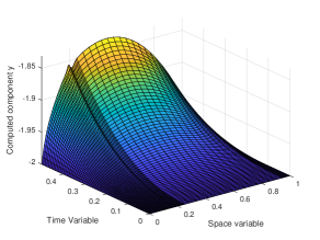
(a) Approximation to $y$

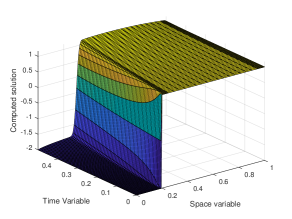
(b) Approximation to $\hat{u}$

Figure 1: Example 1: Numerical approximations to $y$ and $\hat{u}$ with $\varepsilon=2^{-12}$ and $N=M=64$

Table 2: Example 1: Uniform two-mesh global differences and orders of convergence using the numerical method  (18)

	N=M=32	N=M=64	N=M=128	N=M=256	N=M=512	N=M=1024	N=M=2048
$\varepsilon=2^{0}$	3.503E-02	4.546E-02	1.531E-02	5.169E-03	2.067E-03	1.005E-03	4.955E-04
	-0.376	1.570	1.567	1.322	1.041	1.020
$\varepsilon=2^{-1}$	4.422E-02	1.495E-02	5.041E-03	2.017E-03	9.795E-04	4.827E-04	2.396E-04
	1.564	1.569	1.322	1.042	1.021	1.010
$\varepsilon=2^{-2}$	1.426E-02	4.795E-03	1.927E-03	9.318E-04	4.585E-04	2.274E-04	1.132E-04
	1.573	1.315	1.048	1.023	1.012	1.006
$\varepsilon=2^{-4}$	1.986E-03	7.580E-04	3.886E-04	1.967E-04	9.897E-05	4.964E-05	2.486E-05
	1.390	0.964	0.982	0.991	0.996	0.998
$\varepsilon=2^{-6}$	8.317E-03	3.022E-03	9.091E-04	3.251E-04	1.625E-04	8.126E-05	4.063E-05
	1.461	1.733	1.483	1.000	1.000	1.000
$\varepsilon=2^{-8}$	1.610E-02	8.733E-03	3.419E-03	1.081E-03	3.076E-04	1.008E-04	4.369E-05
	0.882	1.353	1.662	1.813	1.610	1.206
$\varepsilon=2^{-10}$	1.325E-02	9.919E-03	5.841E-03	2.769E-03	1.111E-03	4.467E-04	1.897E-04
	0.418	0.764	1.077	1.317	1.315	1.236
$\varepsilon=2^{-12}$	9.178E-03	5.996E-03	3.206E-03	1.437E-03	6.355E-04	3.306E-04	1.718E-04
	0.614	0.903	1.158	1.177	0.943	0.945
$\varepsilon=2^{-14}$	6.754E-03	4.265E-03	2.232E-03	1.121E-03	6.165E-04	3.434E-04	1.895E-04
	0.663	0.934	0.994	0.863	0.844	0.858
	⋮	⋮	⋮	⋮	⋮	⋮	⋮
$\varepsilon=2^{-24}$	5.397E-03	3.502E-03	1.916E-03	1.130E-03	6.769E-04	3.823E-04	2.149E-04
	0.624	0.870	0.762	0.739	0.824	0.831
$\varepsilon=2^{-26}$	5.396E-03	3.501E-03	1.916E-03	1.130E-03	6.770E-04	3.823E-04	2.149E-04
	0.624	0.870	0.761	0.739	0.824	0.831
$D^{N,M}$	4.422E-02	4.546E-02	1.531E-02	5.169E-03	2.067E-03	1.005E-03	4.955E-04
$P^{N,M}$	-0.040	1.570	1.567	1.322	1.041	1.020

Example 2.

Consider the test problem

$$\begin{array}[]{l}-\varepsilon\hat{u}_{ss}+(1+s^{2})\hat{u}_{s}+(s+t)\hat{u}+\hat{u}_{t}=4s(1-s)t+t^{2},\quad(x,t)\in(0,1)\times(0,0.5],\\ u(x,0)=-2,0\leq x<0.1,\quad u(x,0)=1,\ 0.1\leq x\leq 1,\\ u(0,t)=-2,\quad u(1,t)=1,\ 0<t\leq 0.5.\end{array}$$

Note that the source term is present in this example and then problem (26) is approximated with the numerical method (18) on the Shishkin mesh $\bar{Q}^{N,M}.$ For this example, we have

$$I(t)=(\cos t-0.1\sin t)e^{-t^{2}/2}.$$

In addition, observe that $\hat{a}_{s}(d,0)\neq 0$ and $\hat{b}_{s}(d,0)\neq 0$. In Table 3 we see that the numerical approximations converge with almost first order.

Table 3: Example 2: Maximum two-mesh global differences and orders of convergence using the numerical method  (18)

	N=M=32	N=M=64	N=M=128	N=M=256	N=M=512	N=M=1024	N=M=2048
$\varepsilon=2^{0}$	1.978E-01	6.835E-02	3.224E-02	4.361E-02	1.478E-02	4.979E-03	1.984E-03
	1.533	1.084	-0.436	1.561	1.570	1.328
$\varepsilon=2^{-2}$	2.516E-02	3.521E-02	1.235E-02	4.115E-03	1.624E-03	7.870E-04	3.880E-04
	-0.485	1.511	1.585	1.341	1.045	1.020
$\varepsilon=2^{-4}$	1.631E-01	7.441E-02	3.434E-02	1.690E-02	8.342E-03	4.147E-03	2.069E-03
	1.132	1.116	1.023	1.018	1.008	1.003
$\varepsilon=2^{-6}$	3.309E-01	2.423E-01	1.616E-01	7.870E-02	3.916E-02	1.960E-02	9.822E-03
	0.449	0.585	1.038	1.007	0.998	0.997
$\varepsilon=2^{-8}$	3.127E-01	2.284E-01	1.421E-01	7.545E-02	4.301E-02	2.506E-02	1.398E-02
	0.453	0.684	0.913	0.811	0.780	0.842
$\varepsilon=2^{-10}$	3.347E-01	2.251E-01	1.399E-01	7.839E-02	4.277E-02	2.472E-02	1.390E-02
	0.572	0.686	0.836	0.874	0.791	0.830
$\varepsilon=2^{-12}$	3.583E-01	2.367E-01	1.448E-01	8.242E-02	4.451E-02	2.484E-02	1.403E-02
	0.598	0.709	0.813	0.889	0.842	0.824
$\varepsilon=2^{-14}$	3.460E-01	2.450E-01	1.477E-01	8.420E-02	4.566E-02	2.492E-02	1.408E-02
	0.498	0.730	0.811	0.883	0.873	0.824
$\varepsilon=2^{-16}$	3.071E-01	2.240E-01	1.523E-01	8.540E-02	4.605E-02	2.495E-02	1.410E-02
	0.455	0.557	0.834	0.891	0.884	0.824
	⋮	⋮	⋮	⋮	⋮	⋮	⋮
$\varepsilon=2^{-24}$	3.111E-01	2.249E-01	1.391E-01	7.423E-02	4.296E-02	2.495E-02	1.410E-02
	0.468	0.693	0.906	0.789	0.784	0.823
$\varepsilon=2^{-26}$	3.117E-01	2.248E-01	1.391E-01	7.423E-02	4.296E-02	2.495E-02	1.410E-02
	0.471	0.692	0.906	0.789	0.784	0.823
$D^{N,M}$	3.583E-01	2.450E-01	1.616E-01	8.540E-02	4.605E-02	2.506E-02	1.410E-02
$P^{N,M}$	0.548	0.601	0.920	0.891	0.878	0.829

6 Appendix A: A set of singular functions

In this appendix the singular functions $\hat{\psi}_{i},\,i=0,1,2,3,4$ are defined and bounds of their derivatives are given. These functions are the main terms in the regularity expansion (34) of the continuous solution $\hat{u}(s,t)$. These bounds are used in the truncation error analysis of the interior layer component $z$.

For any function $F(x,t)=\hat{F}(s,t)$ we have

$${\cal{L}}F =-\varepsilon F_{xx}+\kappa F_{x}+gF_{t}=-\varepsilon g\hat{F}_{ss}+\left(\sqrt{g}\kappa+g\frac{\partial s}{\partial t}\right)\hat{F}_{s}+g\hat{F}_{t}$$

$$=g\hat{L}_{d}\hat{F}+g\left(\frac{\kappa}{\sqrt{g}}+\frac{\partial s}{\partial t}-a(d,t)\right)\hat{F}_{s},$$

where

$$\hat{L}_{d}\hat{F}:=-\varepsilon\hat{F}_{ss}+\hat{a}(d(t),t)\hat{F}_{s}+\hat{F}_{t}.$$ (27)

Hence, from (5), (6e) and using $\hat{a}(d(t),t)=a(d,t)$ we have

$${\cal{L}}F(x,t)=g\hat{L}_{d}\hat{F}+\sqrt{g}(a(x,t)-a(d,t))\frac{\partial F}{\partial x}.$$ (28)

We will define a set of functions $\{\hat{\psi}_{i}\}_{i=0}^{4}$ such that $\hat{L}_{d}\hat{\psi}_{i}=0$; $\hat{\psi}_{i}\in C^{i-1}(\bar{\hat{Q}}),\ i\geq 1$. Each function $\hat{\psi}_{i}$ is smooth within the open region $\hat{Q}\setminus\Gamma^{*}$. Define the two singular functions [1]

$$\hat{\psi}_{0}(s,t):=\operatorname{erfc}\left(\frac{d(t)-s}{2\sqrt{\varepsilon t}}\right),\quad\hat{E}(s,t):=e^{-\frac{(s-d(t))^{2}}{4\varepsilon t}}.$$ (29)

Then we explicitly write out the derivatives of these two functions

$$\frac{\partial\hat{\psi}_{0}}{\partial s} =\frac{1}{\sqrt{\varepsilon\pi t}}\hat{E},\quad\frac{\partial\hat{E}}{\partial s}=\frac{d(t)-s}{2\varepsilon t}\hat{E},\quad\frac{\partial\hat{E}}{\partial t}=\frac{\sqrt{\pi}(d(t)-s)}{2\sqrt{\varepsilon t}}\frac{\partial\hat{\psi}_{0}}{\partial t};$$

$$\varepsilon\frac{\partial^{2}\hat{\psi}_{0}}{\partial s^{2}} =\frac{d(t)-s}{2t\sqrt{\varepsilon\pi t}}\hat{E},\quad\frac{\partial\hat{\psi}_{0}}{\partial t}=\frac{1}{\sqrt{\varepsilon\pi t}}\left(\frac{(d(t)-s)}{2t}-\hat{a}(d(t),t)\right)\hat{E}.$$

Hence, we have that $\hat{L}_{d}\hat{\psi}_{0}=0.$ Observe that

$$\hat{L}_{d}((d(t)-s)\hat{\psi}_{0}) =2\varepsilon\frac{\partial\hat{\psi}_{0}}{\partial s}=2\frac{\sqrt{\varepsilon}}{\sqrt{\pi t}}\hat{E};\quad\hat{L}_{d}\hat{E}=\frac{1}{2t}\hat{E}$$

$$\hbox{and}\quad\hat{L}_{d}(t^{n+0.5}\hat{E}) =(n+1)t^{n-0.5}\hat{E}\quad\hbox{for all }n\geq 0.$$

We now define the remaining weakly singular functions:

$$\hat{\psi}_{1}(s,t):=(d(t)-s)\hat{\psi}_{0}-2\frac{\sqrt{\varepsilon t}}{\sqrt{\pi}}\hat{E},$$ (30a)

$$\hat{\psi}_{i}=(d(t)-s)\hat{\psi}_{i-1}+2\varepsilon t(i-1)\hat{\psi}_{i-2},\qquad i=2,3,4;$$ (30b)

which satisfy

$$\frac{\partial\hat{\psi}_{i}}{\partial s} =-i\hat{\psi}_{i-1},\quad\hat{L}_{d}\hat{\psi}_{i}=0,\qquad i=1,2,3,4;$$

$$\frac{(-1)^{i}}{i!}\Bigl{[}\frac{\partial^{i}\hat{\psi}_{i}}{\partial s^{i}}\Bigr{]}(d,0) =2,\qquad i=0,1,2,3,4;$$

$$(d(t)-s)\frac{\partial\hat{\psi}_{i}}{\partial s} =-i\hat{\psi}_{i}+2\varepsilon ti(i-1)\hat{\psi}_{i-2}\in C^{i-1}(\bar{\hat{Q}}),\qquad i=2,3,4.$$

Define the parameterized exponential function

$$\hat{E}_{\gamma}(s,t):=e^{-\frac{\gamma(s-d(t))^{2}}{4\varepsilon t}},\qquad 0<\gamma<1.$$

Using the inequality $\operatorname{erfc}(z)\leq Ce^{-z^{2}}\leq Ce^{\gamma^{2}/4}e^{-\gamma z},\,\forall z\geq 0,$ it follows that

$$\Bigl{|}\frac{\partial^{j}}{\partial t^{j}}\hat{\psi}_{0}(s,t)\Bigr{|},\Bigl{|}\frac{\partial^{j}}{\partial t^{j}}\hat{E}(s,t)\Bigr{|}\leq C\left(\frac{1}{t}+\frac{1}{\sqrt{\varepsilon t}}\right)^{j}\hat{E}_{\gamma}(s,t);\quad j=1,2;$$ (31)

Based on the map (5) and the definition of the function $g$ (6f) we have

$$d(t)-s=\sqrt{g}(d-x)\quad\hbox{and}\quad\frac{\partial\psi_{i}}{\partial x}(x,t)=\sqrt{g}\frac{\partial\hat{\psi}_{i}}{\partial s}(s,t).$$

In the transformed domain, the two fundamental functions are:

$$\psi_{0}(x,t):=\operatorname{erfc}\left(\frac{\sqrt{g(t)}(d-x)}{2\sqrt{\varepsilon t}}\right),\qquad E(x,t):=e^{-\frac{g(t)(x-d)^{2}}{4\varepsilon t}}.$$

It follows that

$$\Bigl{|}\frac{\partial^{j}}{\partial t^{j}}\psi_{0}(x,t)\Bigr{|},\Bigl{|}\frac{\partial^{j}}{\partial t^{j}}E(x,t)\Bigr{|}\leq C\left(1+\frac{1}{t}\right)^{j}E_{\gamma}(x,t),\quad j=1,2,\quad x\neq d;$$

$$|\psi_{0}(x,t)|\leq C,\ \Bigl{|}\frac{\partial^{i}}{\partial x^{i}}\psi_{0}(x,t)\Bigr{|},\Bigl{|}\frac{\partial^{i}}{\partial x^{i}}E(x,t)\Bigr{|}\leq C\left(\frac{1}{\sqrt{\varepsilon t}}\right)^{i}E_{\gamma}(s,t),\quad 1\leq i\leq 4.$$

Observe that the bounds on the time derivatives of these two functions do not depend adversely on the singular perturbation parameter $\varepsilon$. This contrasts with the bounds on the time derivatives of these functions in the original variables $(s,t)$.

In the transformed variables, we see from (28) that

$${\cal{L}}\psi_{i}=\sqrt{g}(a(x,t)-a(d,t))\frac{\partial\psi_{i}}{\partial x}\neq 0,\quad\hbox{for}\quad x\neq d.$$

The fact that ${\cal{L}}\psi_{i}\neq 0$, when $\hat{a}$ depends on the spatial variable, results in the function $\hat{y}$ exhibiting an interior layer (see Remark 1.)

The next singular function is

$$\psi_{1}(x,t):=\sqrt{g}(d-x)\psi_{0}-2\frac{\sqrt{\varepsilon t}}{\sqrt{\pi}}E\quad\hbox{and}\quad\frac{\partial\psi_{1}}{\partial x}=-\sqrt{g}\psi_{0}$$ (32a)

and the subsequent three functions are

$$\psi_{i}(x,t):=\sqrt{g}(d-x)\psi_{i-1}+2\varepsilon t(i-1)\psi_{i-2},\quad i=2,3,4.$$ (32b)

As the first space derivatives of these functions are involved in the analysis of the interior layer function, we explicitly record that

$$\frac{\partial\psi_{n}}{\partial x}=-i\sqrt{g}\psi_{n-1},\,n=2,3,4\ \hbox{ and }\ (d-x)^{i}t^{j}\psi_{0}\in C^{2+\gamma}(\bar{Q}),\hbox{ if }i+2j\geq 3.$$

For these singular functions, we can establish the bounds

$$\Bigl{|}\frac{\partial^{j}}{\partial t^{j}}\psi_{1}(x,t)\Bigr{|} \leq C\left(1+\frac{\sqrt{\varepsilon}}{\sqrt{t}}\right)^{j}E_{\gamma}+C,\quad j=1,2;$$

$$\Bigl{|}\frac{\partial}{\partial x}\psi_{1}(x,t)\Bigr{|} \leq C,\quad\Bigl{|}\frac{\partial^{i}}{\partial x^{i}}\psi_{1}(x,t)\Bigr{|}\leq C\left(\frac{1}{\sqrt{\varepsilon t}}\right)^{i-1}E_{\gamma}+C,\quad 2\leq i\leq 4,$$

and

$$\Bigl{|}\frac{\partial}{\partial t}\psi_{n}(x,t)\Bigr{|}\leq C,\quad\Bigl{|}\frac{\partial^{2}}{\partial x^{2}}\psi_{n}(x,t)\Bigr{|}\leq C;\quad n=2,3,4;$$

on the second time derivatives

$$\Bigl{|}\frac{\partial^{2}}{\partial t^{2}}\psi_{2}(x,t)\Bigr{|} \leq C\left(1+\sqrt{\frac{\varepsilon}{t}}\right)^{2}E_{\gamma}(x,t)+C,$$

$$\Bigl{|}\frac{\partial^{2}}{\partial t^{2}}\psi_{3}(x,t)\Bigr{|} \leq C\left(1+\varepsilon\sqrt{\frac{\varepsilon}{t}}\right)E_{\gamma}(x,t)+C;\quad\Bigl{|}\frac{\partial^{2}}{\partial t^{2}}\psi_{4}(x,t)\Bigr{|}\leq CE_{\gamma}(x,t)+C;$$

on the fourth space derivatives

$$\Bigl{|}\frac{\partial^{4}}{\partial x^{4}}\psi_{j}(x,t)\Bigr{|}\leq C(\sqrt{\varepsilon t})^{j-4}E_{\gamma}(x,t)+C,\quad j=2,3,4;$$

and on the third space derivatives

$$\Bigl{|}\frac{\partial^{3}}{\partial x^{3}}\psi_{2}(x,t)\Bigr{|}\leq C\left(1+\frac{1}{\sqrt{\varepsilon t}}\right)E_{\gamma}(x,t)+C;\quad\Bigl{|}\frac{\partial^{3}}{\partial x^{3}}\psi_{n}(x,t)\Bigr{|}\leq C,\quad n=3,4.$$

One can check that for all $m\geq 0,n\geq 1$

$$\hat{L}_{d}(t^{m+0.5}\hat{E})=(m+1)t^{m-0.5}\hat{E}$$ (33a)

$$\hat{L}_{d}(t^{m}(d(t)-s)^{n}\hat{\psi}_{0})$$

$$\hskip 56.9055pt=\bigl{(}mt^{m-1}(d(t)-s)^{n}-\varepsilon n(n-1)t^{m}(d(t)-s)^{n-2}\bigr{)}\hat{\psi}_{0}$$

$$\hskip 56.9055pt+2\sqrt{\frac{\varepsilon}{\pi t}}nt^{m}(d(t)-s)^{n-1}\hat{E}$$ (33b)

$$\hat{L}_{d}(\sqrt{t}(d(t)-s)^{n}\hat{E})$$

$$\hskip 56.9055pt=\left(\frac{(n+1)(d(t)-s)^{n}}{\sqrt{t}}-\varepsilon n(n-1)\sqrt{t}(d(t)-s)^{n-2}\right)\hat{E}$$ (33c)

$$\hat{L}_{d}(t\sqrt{t}(d(t)-s)\hat{E})=3(d(t)-s)\sqrt{t}\hat{E}.$$ (33d)

These expressions will be used to deduce bounds for the component $z_{p}$ in the decomposition (13) of $z$.

In addition, we assume that $a_{x}(d,0)=0$. This guarantees that the component $z_{c}$ of $z$ in (13) satisfies $z_{c}\in C^{4+\gamma}(\bar{Q}^{-})\cup C^{4+\gamma}(\bar{Q}^{+}).$ The regularity of this component comes from observing that $|g-1|\leq Ct$ and so

$$(d-x)(g-1),\ t(g-1)\psi_{0},\ (d-x)^{2}(g-1)\psi_{0}\in C^{2+\gamma}(\bar{Q}).$$

Thus, from (28), (32a), (32b) and the assumption $a_{x}(d,0)=0$, we have

$${\cal{L}}\psi_{i}=-ig\bigl{(}a(d,t)-a(x,t)\bigr{)}\psi_{i-1}\in C^{2+\gamma}(\bar{Q}),\ i\geq 2,$$

which is used in (35) in Appendix C.

7 Appendix B: Decomposition of the solution

In this appendix we decompose the solution of problem (2) into a regular $\hat{v}$, boundary layer $\hat{w}$ and interior layer $\hat{z}$ components. Bounds for the derivatives of $\hat{v}$ and $\hat{w}$ are established here and the bounds for the component $z$ in Appendix C.

We have the following expansion for the solution of problem (2):

$$\hat{u}(s,t)=0.5\sum_{i=0}^{4}[\phi^{(i)}](d)\frac{(-1)^{i}}{i!}\hat{\psi}_{i}(s,t)+\hat{R}(s,t),\qquad\hat{R}\in C^{4+\alpha}(\bar{\hat{Q}});$$ (34)

and, as we have assumed that $[\phi^{\prime}](d)=0$, then

$$\hat{y}(s,t)=0.5\sum_{i=2}^{4}[\phi^{(i)}](d)\frac{(-1)^{i}}{i!}\hat{\psi}_{i}(s,t)+\hat{R}(s,t).$$

Note that the smooth remainder $\hat{R}$ satisfies the singularly perturbed problem

$$\hat{L}\hat{R} =\hat{f}-0.5\sum_{i=0}^{4}[\phi^{(i)}](d)\frac{(-1)^{i}}{i!}\hat{L}\hat{\psi}_{i}(s,t),\ (s,t)\in\hat{Q};$$

$$\hat{R}(s,0) =\hat{y}(s,0)-0.5\sum_{i=2}^{4}[\phi^{(i)}](d)\frac{(-1)^{i}}{i!}\hat{\psi}_{i}(s,0),\ 0\leq s\leq 1;$$

$$\hat{R}(p,t) =\hat{y}(p,t)-0.5\sum_{i=2}^{4}[\phi^{(i)}](d)\frac{(-1)^{i}}{i!}\hat{\psi}_{i}(p,t),\quad t>0;\ p=0,1.$$

This can be further decomposed as follows

$$\hat{R}=\hat{v}+\hat{w}+\hat{z},\quad\hat{v},\hat{w}\in C^{4+\alpha}(\bar{\hat{Q}});$$

where

$$\hat{L}\hat{v} =\hat{f},\quad\hat{L}\hat{w}=0,\quad\hat{L}\hat{z}=\hat{L}\hat{R}-\hat{f};\quad(s,t)\in\hat{Q};$$

$$\hat{v}(0,t) =\hat{R}(0,t),\quad\hat{v}(s,0)=\hat{R}(s,0),\quad\hat{v}(1,t)=\hat{v}^{*}(1,t);$$

$$\hat{w}(0,t) =0,\quad\hat{w}(s,0)=0,\quad\hat{w}(1,t)=(\hat{R}-\hat{v}^{*})(1,t);$$

$$\hat{z}(0,t) =0,\quad\hat{z}(s,0)=0,\quad\hat{z}(1,t)=0.$$

As in [7], the outflow boundary values for $\hat{v}$ can be specified (they are denoted by $\hat{v}^{*}(1,t)$ above) so that we have the following bounds

$$\left|\frac{\partial^{i+j}}{\partial s^{i}\partial t^{j}}\hat{v}(s,t)\right| \leq C,\ 0\leq i+j\leq 2,\qquad\left|\frac{\partial^{3}}{\partial s^{3}}\hat{v}(s,t)\right|\leq C\left(1+\frac{1}{\varepsilon}\right),$$

$$\left|\frac{\partial^{i+j}}{\partial s^{i}\partial t^{j}}\hat{w}(s,t)\right| \leq C\varepsilon^{-i}(1+\varepsilon^{1-j})e^{-\alpha(1-s)/\varepsilon},\quad 0\leq i+2j\leq 4.$$

8 Appendix C: Regularity and bounds on the interior layer function

To obtain sharp bounds on the derivatives of the interior layer component $\hat{z}$, we transform the problem $\hat{L}\hat{z}(s,t)=\hat{L}\hat{R}(s,t)-\hat{f}$ to the $(x,t)$ coordinate system. In this appendix bounds for the two subcomponents $z_{c}$ and $z_{p}$ in the decomposition (13) of $z$ are established. In the case of the component $z_{p}$, they are established using a further decomposition into two components $z_{q}$ and $z_{R}$. By the definition (14) of the subcomponent $z_{c}$, we have

$${\cal{L}}z_{c}(x,t) =-\frac{g}{2}\bigl{(}a(d,t)-a(x,t)\bigr{)}\sum_{i=1}^{3}[\phi^{(i+1)}](d)\frac{(-1)^{i}}{i!}\psi_{i}(x,t)$$

$$=:F_{c}(x,t)\in C^{2+\gamma}(\bar{Q});$$ (35)

and, hence,

$$z_{c}\in C^{4+\gamma}(\bar{Q}^{-})\cup C^{4+\gamma}(\bar{Q}^{+}).$$

The function $z_{c}$ is sufficiently regular within each sub-domain to allow us use results from [9] to bound the derivatives of $z_{c}$. In the stretched variable

$$\zeta=\frac{x-d}{\sqrt{\varepsilon}},$$

we have the bounds

$$|{\cal{L}}z_{c}(\zeta,t)| \leq C\sqrt{\varepsilon}e^{-\frac{\gamma g\zeta^{2}}{4t}},$$ (36a)

$$\Bigl{|}\frac{\partial^{i+j}({\cal{L}}z_{c}(\zeta,t))}{\partial\zeta^{i}\partial t^{j}}\Bigr{|} \leq C\varepsilon^{i/2}e^{-\frac{\gamma g\zeta^{2}}{4t}},\quad 1\leq i+2j\leq 2.$$ (36b)

These bounds are used in Theorem 2 to deduce estimates for the component $z_{c}$ and some of its partial derivatives.

We next examine the regularity of the subcomponent $z_{p}(x,t)$, which is defined as the solution of problem (15). From assumption (2g) we have the following Taylor expansion

$$a(d,t)-a(x,t)=p_{d}(x,t)+r_{1}(x,t),$$

$$p_{d}(x,t):=-\left[a_{xx}(d,0)\frac{(d-x)^{2}}{2!}+a_{xxx}(d,0)\frac{(d-x)^{3}}{3!}+t(d-x)a_{xt}(d,0)\right],$$

$$r_{1}(x,t):=K_{0}(d-x)^{4}+K_{1}t(d-x)^{2}+K_{2}t(d-x)^{3}+K_{3}t^{2}(d-x).$$

Once again, this interior layer component $z_{p}$ is decomposed into the sum

$$z_{p}(x,t) :=z_{q}(x,t)+z_{R}(x,t),$$ (37)

$$z_{q}(x,t) =B_{1}\sqrt{t}(g(d-x)^{2}+\varepsilon t)E,$$

$$+B_{2}\sqrt{gt}(d-x)(g(d-x)^{2}+2\varepsilon t)E+B_{3}t\sqrt{gt}(d-x)E.$$ (38)

The constants $B_{1},B_{2}$ and $B_{3}$ are given by

$$B_{1}:=-\frac{a_{xx}(d,0)}{3!\sqrt{\varepsilon\pi}},\ B_{2}:=\frac{a_{xxx}(d,0)}{4!\sqrt{\varepsilon\pi}},\ B_{3}:=\frac{a_{xt}(d,0)}{3\sqrt{\varepsilon\pi}}.$$

Note that $z_{q}\in C^{2+\gamma}(\bar{Q}^{-})\cup C^{2+\gamma}(\bar{Q}^{+})$ and

$$z_{q}(d,t)=\varepsilon B_{1}t\sqrt{t},\ [z_{q}](d,t)=0,\quad\Bigl{[}\frac{1}{\sqrt{g}}\frac{\partial z_{q}}{\partial x}\Bigr{]}(d,t)=0,\quad z_{q}(x,0)=0.$$

Using that $\operatorname{erfc}(z)\leq Ce^{-z^{2}},\forall z$, we can establish the bounds

$$\Bigl{|}\frac{\partial^{i}z_{q}}{\partial x^{i}}(x,t)\Bigr{|} \leq C(\sqrt{\varepsilon})^{-i}\bigl{(}\sqrt{\varepsilon}+|a_{xt}(d,0)|\bigr{)}E_{\gamma}(x,t),\quad i=0,1,2,3;$$ (39a)

$$\Bigl{|}\frac{\partial^{j}z_{q}}{\partial t^{j}}(x,t)\Bigr{|} \leq C(|a_{xt}(d,0)|+\sqrt{\varepsilon}(\sqrt{t})^{1-j})E_{\gamma}(x,t),\quad j=1,2,$$ (39b)

$$\Bigl{|}\frac{\partial^{2}z_{q}}{\partial x\partial t}(x,t)\Bigr{|} \leq C(\sqrt{\varepsilon})^{-1}\bigl{(}\sqrt{\varepsilon}+|a_{xt}(d,0)|\bigr{)}E_{\gamma}(x,t).$$ (39c)

By the choice of constants $B_{1},B_{2},B_{3}$ and using the expressions (33a), (33c), (33d) (28), we see that $z_{p}(x,t)$ satisfies

$${\cal{L}}z_{p}(x,t) =p_{d}(x,t)\frac{g}{\sqrt{\varepsilon\pi t}}E(x,t)+r_{2}(x,t)+{\cal{L}}z_{R}(x,t),\quad\hbox{where}$$

$$r_{2}(x,t) :=(\tilde{p}_{d}-p_{d})(x,t)\frac{g}{\sqrt{\varepsilon\pi t}}E(x,t)+\sqrt{g}(a(x,t)-a(d,t))\frac{\partial z_{q}}{\partial x}$$ (40)

and

$$\tilde{p}_{d}(x,t):=-\left[a_{xx}(d,0)\frac{g(d-x)^{2}}{2!}+a_{xxx}(d,0)\frac{g\sqrt{g}(d-x)^{3}}{3!}+t\sqrt{g}(d-x)a_{xt}(d,0)\right].$$

The function $p_{d}$ and the related function $\tilde{p}_{d}$ satisfy

$$|\tilde{p}_{d}(x,t)-p_{d}(x,t)|\leq C|(g-1)(d-x)|\bigl{(}|d-x|+t|a_{xt}(d,0)|\bigr{)}.$$

By the definitions (15) of $z$ and (14) of the subcomponent $z_{c}$ we have

$${\cal{L}}z_{R} =r_{1}(x,t)\frac{g}{\sqrt{\varepsilon\pi t}}E(x,t)-r_{2}(x,t)=:F_{R}(x,t)\in C^{2+\gamma}(\bar{Q});$$

$$z_{R}(x,0) =0;\ [z_{R}](d,t)=0,\quad[(z_{R})_{x}](d,t)=0;$$

$$z_{R}(0,t) =K_{4}\frac{\sqrt{t}}{\sqrt{\varepsilon}}e^{-\frac{gd^{2}}{\varepsilon t}},z_{R}(1,t)=K_{5}\frac{\sqrt{t}}{\sqrt{\varepsilon}}e^{-\frac{g(1-d)^{2}}{\varepsilon t}},$$

where the values of $K_{4}$ and $K_{5}$ can be obtained from (38). Hence, the function $z_{R}$ is sufficiently regular within each sub-domain to allow us use results from [9] to bound the derivatives of $z_{R}$. That is,

$$z_{R}\in C^{4+\gamma}(\bar{Q}^{-})\cup C^{4+\gamma}(\bar{Q}^{+}).$$

Moreover, using $|\sqrt{g}-1|\leq|g-1|$ and $|g-1|\leq Ct,$ we conclude that,

$$|{\cal{L}}z_{R}(x,t)|\leq CE_{\gamma}(x,t)\leq Ce^{-\frac{|x-d|}{2\sqrt{\varepsilon t}}},\quad x\neq d.$$

In the stretched variable

$$\zeta=\frac{x-d}{\sqrt{\varepsilon}},$$

we have that

$$\Bigl{|}\frac{\partial^{i+j}({\cal{L}}z_{R}(\zeta,t))}{\partial\zeta^{i}\partial t^{j}}\Bigr{|}\leq Ce^{-\frac{\gamma g\zeta^{2}}{4t}},\quad 0\leq i+2j\leq 2.$$ (41)

References

[1] L. Bobisud, Parabolic equations with a small parameter and discontinuous data, J. Math. Anal. Appl., 26, 1969, 208–220.
[2] P.A. Farrell, A.F. Hegarty, J.J.H. Miller, E. O’Riordan and G.I. Shishkin, Robust computational techniques for boundary layers,
CRC Press, 2000.
[3] N. Flyer and B. Fornberg, Accurate numerical resolution of transients in initial-boundary value problems for the heat equation, J. Comp. Physics184, 526–539, (2003).
[4] A. Friedman, Partial differential equations of parabolic type, Prentice-Hall, Englewood Cliffs, N.J., 1964.
[5] J.L. Gracia and E. O’Riordan, A singularly perturbed convection–diffusion problem with a moving interior layer, Int. J. Num. Anal. Mod., v. 9 (4), (2012), 823–843.
[6] J.L. Gracia and E. O’Riordan, Numerical approximations to a singularly perturbed convection-diffusion problem with a discontinuous initial condition, Arxiv.
[7] J.L. Gracia and E. O’Riordan, Numerical approximation of solution derivatives of singularly perturbed parabolic problems of convection–diffusion type, Math. Comput., v. 85, (2016), 581–599.
[8] J.L. Gracia and E. O’Riordan, Parameter-uniform numerical methods for singularly perturbed parabolic problems with incompatible boundary-initial data, Appl. Numer. Math., v. 146, (2019), 436–451.
[9] O.A. Ladyzhenskaya, V.A. Solonnikov and N.N. Ural’tseva, Linear and quasilinear equations of parabolic type, Transactions of Mathematical Monographs, 23, American Mathematical Society, 1968.
[10] G.I. Shishkin, Grid approximation of singularly perturbed parabolic convection-diffusion equations with a piecewise-smooth initial condition, Zh. Vychisl. Mat. Mat. Fiz., v. 46 (1), (2006), 52–76.
[11] G.I. Shishkin and L.P. Shishkina, Difference methods for singular perturbation problems, CRC Press, 2009.
[12] M. Stynes and E. O’Riordan, A uniformly convergent Galerkin method on a Shishkin mesh for a convection-diffusion problem, J. Math. Anal. Appl., v. 214, (1997), 36–54.
[13] U.Kh. Zhemukhov, Parameter-uniform error estimate for the implicit four-point scheme for a singularly perturbed heat equation with corner singularities, Translation of Differ. Uravn. v. 50 (7) (2014), v. 7, 923–936; Differ. Equ. v. 50 (7), (2014), 913–926.