Numerical approximations to a singularly perturbed convection-diffusion problem with a discontinuous initial condition

Abstract

A singularly perturbed parabolic problem of convection-diffusion type with a discontinuous initial condition is examined. An analytic function is identified which matches the discontinuity in the initial condition and also satisfies the homogenous parabolic differential equation associated with the problem. The difference between this analytical function and the solution of the parabolic problem is approximated numerically, using an upwind finite difference operator combined with an appropriate layer-adapted mesh. The numerical method is shown to be parameter-uniform. Numerical results are presented to illustrate the theoretical error bounds established in the paper.

Keywords: Convection diffusion, discontinuous initial condition, interior layer, Shishkin mesh.

AMS subject classifications: 65M15, 65M12, 65M06

1 Introduction

In this paper, we examine a singularly perturbed convection-diffusion problem with a discontinuous initial condition. Throughout, we assume that the convective coefficient multiplying the first spatial derivative of the solution (denoted below by $u(x,t)$) is smooth, strictly positive and depends solely on the time variable $t$. Under this assumption, an explicit discontinuous function (denoted below by $S(x,t)$) can be identified which captures the nature of the singularity associated with the discontinuous initial condition. Asymptotic expansions for the solution $u(x,t)$, involving this singularity, were constructed in [1]. When we subtract off this singular function the remainder $y(x,t):=u(x,t)-S(x,t)$ is again the solution of a singularly perturbed convection-diffusion problem. However, although the remainder $y$ satisfies the same singularly perturbed partial differential equation as $u$, the initial condition $y(x,0)$ is now continuous. In this paper, we construct and analyze a numerical method that produces parameter-uniform [2] numerical approximations to this remainder $y$.

In [7], we examined a set of related singularly perturbed reaction-diffusion problems with discontinuities in either the boundary or the initial condition. In this paper, we extend this technique to a convection-diffusion problem with a discontinuous initial condition. In this case, the location of the interior layer (generated by the discontinuity in the initial condition) moves in time and, in addition, this interior layer can eventually merge into a boundary layer.

Shishkin [9] constructed and analysed a numerical method for the problem examined below, in the case where the initial condition is continuous, but has a discontinuity in the first derivative. The error bound in [9, (5.23)] essentially coincides with the error bound presented below in Theorem 1. Hence, the presence of the complimentary error function in the problem formulated here does not significantly alter the final error bound established in [9, Theorem 8].

In the more general case where the convective coefficient can depend on both space and time, remainder $y$ contains a strong interior layer and the numerical algorithm presented in this paper will not suffice (see Example 5 in §4.2) to generate parameter-uniform approximations. In a companion paper [5] to the current paper, we present a different numerical algorithm to manage this more general case. Here we show that a simpler algorithm (to the algorithm in [5]) suffices when the convective coefficient does not depend on the spatial variable $x$.

In §2, we define the continuous problem to be examined, define the singular function $S(x,t)$ and present a priori bounds on the derivatives of the remainder term $y(x,t)$. In §3, we construct a numerical method and establish a parameter-uniform error bound on the associated numerical approximations. In §4, we present some numerical results to illustrate the performance of the numerical method and to support the theoretical error bounds. Some technical details are available in the Appendix.

Notation: Throughout the paper, $C$ denotes a generic constant that is independent of the singular perturbation parameter $\varepsilon$ and all the discretization parameters. The $L_{\infty}$ norm on the domain $D$ will be denoted by $\|\cdot\|_{D}$. We also define the jump of a function at a point $d$ by $[\phi](d):=\phi(d^{+})-\phi(d^{-})$.

2 Continuous problem

Consider the following singularly perturbed parabolic convection-diffusion problem: Find $u$ such that

$$Lu:=-\varepsilon{u}_{xx}+a(t){u}_{x}+{u}_{t}=0,\quad(x,t)\in Q:=(0,1)\times(0,T],$$ (1a)

$${u}(x,0)=\phi(x),\,0\leq x\leq 1;\ [\phi](d)\neq 0,\ 0<d=O(1)<1;$$ (1b)

$${u}(0,t)=0={u}(1,t),\ 0<t\leq T,$$ (1c)

$$a(t)>\alpha>0,\ 0\leq t\leq T,\quad a\in C^{4+\gamma}(\bar{Q}),$$ (1d)

$$\ \ \phi\in C^{4}((0,1)\setminus\{d\});\qquad\phi^{(2i)}(0)=\phi^{(2i)}(1)=0;\quad i=0,1,2.$$ (1e)

The assumption of the compatibility conditions (1e) ensures that no classical singularity appears near the end points $(0,0),(1,0)$. Observe that the initial function $\phi(x)$ is discontinuous at $x=d$. This will cause an interior layer to appear in the solution, near the point $(d,0)$, which will be convected into the interior of the domain along the characteristic curve

$$\Gamma^{*}:=\{(d(t),t)|\,d^{\prime}(t)=a(t),\ 0<d(0)=d<1\}$$

associated with the reduced first order differential equation. Define the continuous function

$$y(x,t):=u(x,t)-S(x,t),\qquad S(x,t):=0.5[\phi](d)\psi_{0}(x,t),$$ (2)

where

$$\psi_{0}(x,t):=\operatorname{erfc}\left(\frac{d(t)-x}{2\sqrt{\varepsilon t}}\right)\quad\hbox{and}\quad\operatorname{erfc}(z):=\frac{2}{\sqrt{\pi}}\int_{r=z}^{\infty}e^{-r^{2}}\ dr.$$

This function $y$ satisfies the problem

$$Ly=0,\ (x,t)\in Q,\qquad y(x,0)=\left\{\begin{array}[]{lll}\displaystyle\phi(x),&x<d,\\[4.30554pt] \displaystyle\phi(d^{-}),&x=d,\\[4.30554pt] \displaystyle\phi(x)-[\phi](d),&x>d.\end{array}\right.$$ (3d)

$$y(0,t)=-0.5[\phi](d)\psi_{0}(0,t),\quad 0<t\leq T,$$ (3e)

$$y(1,t)=-0.5[\phi](d)\psi_{0}(1,t),\quad 0<t\leq T.$$ (3f)

As $d=O(1)$ we see that all time derivatives of the left boundary condition $y(0,t)$ are uniformly bounded. To begin, we shall assume that the final time $T$ is constrained as follows: there exists some $\delta>0$ such that

$$d(T)\leq 1-\delta.$$ (4)

In §3.2, we explain what modifications are required in the numerical method when this constraint is not applied. Note that, by assuming (4), all time derivatives of the right boundary condition $y(1,t)$ are uniformly bounded (w.r.t. $\varepsilon$) for all $t\leq T$.

From the Appendix, we have the expansion (23)

$$y=0.5\sum_{i=1}^{4}[\phi^{(i)}](d)\frac{(-1)^{i}}{i!}\psi_{i}(x,t)+R(x,t),\quad\psi_{i}\in C^{i-1+\gamma}(\bar{Q}),$$

where the weakly singular functions $\psi_{i}$ are defined by (20), (21) and (22). Bounds on the partial derivatives of the function $\psi_{i}(x,t),i=1,2,3,4$ are stated in (24), (25). In the case where the convective coefficient $a$ is independent of the space variable, we have that

$$L\psi_{i}=0,\quad 0\leq i\leq 4\ \hbox{ and }$$

$$LR(x,t)=0,\ (x,t)\in Q,\ R(x,t)\neq 0,\ (x,t)\in\partial Q.$$

As $R(x,0)\in C^{4}(0,1)$ we also have

$$R\in C^{4+\gamma}(\bar{Q}).$$

Following the arguments in [6, Theorem 1], we have the following decomposition of the smooth remainder

$$R=v_{R}+w$$

into a regular component $v_{R}$ and a boundary layer component $w$. In addition, assuming (4), we have the following bounds

$$\left\|\frac{\partial^{i+j}v_{R}}{\partial x^{i}\partial t^{j}}\right\|_{\bar{Q}} \leq C,\ 0\leq i+j\leq 2,\qquad\left\|\frac{\partial^{3}v_{R}}{\partial x^{3}}\right\|_{\bar{Q}}\leq\frac{C}{\varepsilon},$$ (5a)

$$\left|\frac{\partial^{i+j}}{\partial x^{i}\partial t^{j}}w(x,t)\right| \leq C\varepsilon^{-i}(1+\varepsilon^{1-j})e^{-\alpha(1-x)/\varepsilon},\quad 0\leq i+2j\leq 4.$$ (5b)

Then, combining these bounds with the bounds on the singular functions $\psi_{i}$ (see (24), (25) in the Appendix for details), we have, assuming (4),

$$y =v+w-0.5[\phi^{\prime}](d)\psi_{1}(x,t),$$ (6a)

$$\hbox{where}\qquad v :=v_{R}+0.5\sum_{i=2}^{4}[\phi^{(i)}](d)\frac{(-1)^{i}}{i!}\psi_{i}(x,t)\$$ (6b)

$$\hbox{and}\qquad\left\|\frac{\partial^{i+j}v}{\partial x^{i}\partial t^{j}}\right\|_{\bar{Q}} \leq C,\quad 0\leq i+2j\leq 2,$$ (6c)

$$\left|\frac{\partial^{2}}{\partial t^{2}}v(x,t)\right|\leq C\left(1+\frac{\varepsilon}{t}\right), \left|\frac{\partial^{3}}{\partial x^{3}}v(x,t)\right|\leq C\left(\frac{1}{\varepsilon}+\frac{1}{\sqrt{\varepsilon t}}\right).$$ (6d)

Remark 1.

If $[\phi^{\prime}](d)=0$, then the function $y$ is decomposed simply as $y=v+w$ and this will have an influence on the order of convergence of the numerical scheme (7). In this case, it is proved in Theorem 1 that the method converges with almost first order. Otherwise, when $[\phi^{\prime}](d)\neq 0$, the error bound is dominated by the term $CM^{-1/2}$, which corresponds to the result in [9].

3 Numerical method and associated error analysis

In this section problem (3) is approximated using the backward Euler method and standard central differences on a Shishkin mesh [2]. Global parameter-uniform error bounds are proved for this scheme. Two cases are considered in our error analysis: In §3.1 the interior layer does not interact with the boundary layer at $x=1$ but it does interact in §3.2.

3.1 Interior and boundary layers do not interact with each other

In this section we assume that (4) is satisfied. Then, the interior layer emanating from $x=d$ and travelling along the characteristic $\Gamma^{*}$ does not interact with the boundary layer in the vicinity of $x=1.$

Let $N$ and $M=O(N)$ be two positive integers. We approximate problem (1) with a finite difference scheme on a mesh $\bar{Q}^{N,M}=\{x_{i}\}^{N}_{i=0}\times\{t_{j}\}_{j=0}^{M}$. We denote by $\partial Q^{N,M}:=\bar{Q}^{N,M}\backslash Q.$ The mesh $\bar{Q}^{N,M}$ incorporates a uniform mesh ($t_{j}:=kj$ with $k=T/M$) for the time variable and a piecewise-uniform mesh for the space variable with $h_{i}:=x_{i}-x_{i-1}$. The piecewise uniform mesh $\{x_{i}\}^{N}_{i=0}$ is a Shishkin mesh [2] which splits the interval $[0,1]$ into the two subintervals

$$[0,1-\sigma]\cup[1-\sigma,1],\quad\hbox{where}\quad\sigma:=\min\left\{0.5,\frac{\varepsilon}{\alpha}\ln N\right\}.$$

The $N$ space mesh points are distributed in the ratio $N/2:N/2$ across the two subintervals. The discrete problem is: Find $Y$ such that

$$L^{N,M}Y :=-\varepsilon\delta^{2}_{x}Y+aD^{-}_{x}Y+D^{-}_{t}Y=0,\quad t_{j}>0,$$ (7a)

$$Y(x_{i},0) =y(x_{i},0),\ 0<x_{i}<1,\ Y(0,t_{j})=Y(1,t_{j})=0,\ t_{j}\geq 0.$$ (7b)

Remark 2.

The method and the analysis presented here for problem (1) can be easily extended to a wider class of problems. Consider the more general problem

$$L_{g}u:=-\varepsilon{u}_{xx}+a(t){u}_{x}+b(t){u}+{u}_{t}=f,\ (x,t)\in Q,$$ (8a)

$$u=g\in\partial Q:=\bar{Q}\setminus Q,\quad[u](d,0)\neq 0;$$ (8b)

$$b(t)\geq 0,\ 0\leq t\leq T.$$ (8c)

As the problem is linear we can write the solution as the sum

$$u =e^{-\int_{0}^{t}b(r)dr}u_{h}+u_{p},\quad\hbox{where}$$

$$Lu_{h} =0,\qquad L_{g}u_{p}=f,(x,t)\in Q;$$

$$u_{h}(x,0) =\phi(x);\quad u_{p}(x,0)=u(x,0)-\phi(x);$$

$$u_{h}(0,t) =u_{h}(1,t)=0;\quad u_{p}(0,t)=u(0,t),\ u_{p}(1,t)=u(1,t).$$

In addition to the constraint (1d), we assume that $b,f$ are sufficiently regular and that sufficient compatibility is imposed at the points $(0,0),(1,0)$ so that $u_{p}\in C^{4+\gamma}(\bar{Q})$. The component $u_{h}$ satisfies problem (1) and it will examined below. The component $u_{p}$ can be decomposed into a regular and boundary layer component as in [10]. For problem (8), we first subtract off the term

$$y(x,t):=u(x,t)-S_{g}(x,t),\qquad S_{g}(x,t):=0.5[\phi](d)e^{-\int_{0}^{t}b(r)dr}\psi_{0}(x,t),$$

then $L_{g}y=f,(x,t)\in Q$ and $y=u-S_{g},\ (x,t)\in\partial Q$. The corresponding discrete problem is then given by

$$L_{g}^{N,M}Y :=-\varepsilon\delta^{2}_{x}Y+aD^{-}_{x}Y+bY+D^{-}_{t}Y=f,\quad(x_{i},t_{j})\in Q^{N,M},$$

$$Y(x_{i},0) =y(x_{i},0),\quad(x_{i},t_{j})\in\partial Q^{N,M};$$

where the mesh $Q^{N,M}$ is as described earlier.

We form a global approximation $\bar{Y}$ using simple bilinear interpolation:

$$\bar{Y}(x,t):=\sum_{i=0,j=1}^{N,M}Y(x_{i},t_{j})\varphi_{i}(x)\eta_{j}(t)$$

where $\varphi_{i}(x)$ is the standard hat function centered at $x=x_{i}$ and $\eta_{j}(t):=(t-t_{j-1})/k,\,t\in[t_{j-1},t_{j}),\,\eta_{j}(t):=0,\,t\not\in[t_{j-1},t_{j})$.

Theorem 1.

Assume (4) and $M=O(N)$. If $Y$ is the solution of (7) and $y$ is the solution of (3), then

$$\|\bar{Y}-y\|_{\bar{Q}}\leq CN^{-1}\ln N+C|[\phi^{\prime}](d)|M^{-1/2}.$$

Proof.

As in the case of the continuous problem, the discrete solution can be decomposed into the sum $Y=V+W-0.5\ [\phi^{\prime}](d)\Psi$, where

$$L^{N,M}V =Lv,\ (x_{i},t_{j})\in{Q^{N,M}}\quad\hbox{and}\quad V=v,\ ({x_{i}},t_{j})\in{\partial Q^{N,M};}$$

$$L^{N,M}W =0,\ (x_{i},t_{j})\in{Q^{N,M}}\quad\hbox{and}\quad W=w,\ ({x_{i}},t_{j})\in{\partial Q^{N,M};}$$

$$L^{N,M}\Psi =0,\ (x_{i},t_{j})\in{Q^{N,M}}\quad\hbox{and}\quad\Psi=\psi_{1},\ ({x_{i}},t_{j})\in{\partial Q^{N,M}.}$$

Using the bounds on the derivatives (5b) of the component $w$, truncation error bounds, discrete maximum principle, a suitable discrete barrier function and following the arguments in [8], we can establish the following bounds

$$|(w-W)(x_{i},t_{j})|\leq CN^{-1}\ln N+CM^{-1},\quad(x_{i},t_{j})\in\bar{Q}^{N,M}.$$ (10)

We next bound the error due to the regular component $v$. Note that if the truncation error is denoted by ${\cal T}_{i,j}:=L^{N,M}(v-V)(x_{i},t_{j})$, then

$$|{\cal T}_{i,j}| \leq C\varepsilon(h_{i}+h_{i+1})\left\|\frac{\partial^{3}v(x,t_{j})}{\partial x^{3}}\right\|_{(x_{i-1},x_{i+1})}$$

$$+C\min\left\{h_{i}\left\|\frac{\partial^{2}v(x,t_{j})}{\partial x^{2}}\right\|_{(x_{i-1},x_{i})},\left\|\frac{\partial v(x,t_{j})}{\partial x}\right\|_{(x_{i-1},x_{i})}\right\}$$

$$+C\min\left\{\frac{1}{k}\int_{w=t_{j-1}}^{t_{j}}\int_{r=w}^{t_{j}}\left|\frac{\partial^{2}v(x_{i},r)}{\partial t^{2}}\right|dr\ dw,\left\|\frac{\partial v(x_{i},t)}{\partial t}\right\|_{(t_{j-1},t_{j})}\right\},$$

as

$$|D_{t}^{-}v(x_{i},t_{j})|\leq\frac{1}{k}\int_{r=t_{j-1}}^{t_{j}}\left|\frac{\partial v(x_{i},r)}{\partial r}\ dr\right|\leq C\left\|\frac{\partial v(x_{i},t)}{\partial t}\right\|_{(t_{j-1},t_{j})}.$$

Hence, using the bounds (6) on the derivatives of $v$, we obtain

$$|{\cal T}_{i,1}| \leq C\qquad\hbox{and}$$ (11a)

$$|{\cal T}_{i,j}| \leq C\left(1+\frac{\sqrt{\varepsilon}}{\sqrt{t_{j}}}\right)N^{-1}+Ck\left\|\frac{\partial^{2}v(x_{i},t)}{\partial t^{2}}\right\|_{(t_{j-1},t_{j})}$$

$$\leq C\left(1+\frac{\sqrt{\varepsilon}}{\sqrt{t_{j}}}\right)N^{-1}+CM^{-1}\left(1+\frac{\varepsilon}{t_{j-1}}\right),\quad t_{j}>t_{1}.$$ (11b)

We now mimic the argument in [12] and note that at each time level,

$$\left(-\varepsilon\delta^{2}_{x}+aD^{-}_{x}+\frac{1}{k}I\right)(v-V)(x_{i},t_{j})={\cal T}_{i,j}+\frac{1}{k}(v-V)(x_{i},t_{j-1}),\ t_{j}>0.$$

From this and (11), we deduce the error bound

$$|(v-V)(x_{i},t_{j})| \leq Ck\sum_{n=1}^{j}|{\cal T}_{i,n}|\leq CM^{-1}+k\sum_{n=2}^{j}|{\cal T}_{i,n}|$$

$${\leq C(N^{-1}+M^{-1})+CM^{-3/2}\sqrt{\varepsilon}\int_{s=1}^{j}\frac{ds}{\sqrt{s}}+CM^{-1}\varepsilon\int_{s=1}^{j}\frac{ds}{s}}$$

$$\leq CN^{-1}+CM^{-1}(1+\varepsilon\ln(1+j))$$

$$\leq CN^{-1}+CM^{-1}(1+\varepsilon\ln M).$$ (12)

Finally, we consider the error due to the weakly singular component $\psi_{1}$. Its truncation error is denoted by ${\cal\widetilde{T}}_{i,j}:=L^{N,M}(\psi_{1}-\Psi)(x_{i},t_{j})$. The argument splits into the two cases of $\varepsilon\leq CM^{-1}$ and $\varepsilon\geq CM^{-1}$. In the first case, where $\varepsilon\leq CM^{-1}$, using the bound (24d) on the first time derivative of $\psi_{1}$ at $t=t_{1}$, we have

$$|{\cal\widetilde{T}}_{i,1}| \leq C\frac{N^{-1}}{k}+Ca(t_{1})+C\frac{1}{k}\int_{r=0}^{k}\left(1+\sqrt{\frac{\varepsilon}{r}}\right)\ dr$$

$$\leq C\frac{N^{-1}}{k}+C.$$ (13)

For $t_{j}>t_{1},$ we first sharpen our bounds on the function $\psi_{1}$. Observe that

$$|\psi_{0}(x,t)|\leq CE(x,t),\qquad\hbox{if}\quad x\leq d(t),$$

$$|\psi_{1}(x,t)-2(d(t)-x))|=\left|(d(t)-x)(\psi_{0}-2)-2\frac{\sqrt{\varepsilon t}}{\sqrt{\pi}}E\right|$$

$$\hskip 42.67912pt\leq CE(x,t),\qquad\hbox{if}\quad x\geq d(t).$$

Hence, instead of (24d), (24f) on the first derivatives of $\psi_{1}$, we have the following derivative bounds:

$$\left|\frac{\partial}{\partial t}\psi_{1}(x,t)\right| \leq C\left(1+\sqrt{\frac{\varepsilon}{t}}\right)E(x,t),\ x\leq d(t),$$

$$\left|\frac{\partial}{\partial t}(\psi_{1}(x,t)-2(d(t)-x))\right| \leq C\left(1+\sqrt{\frac{\varepsilon}{t}}\right)E(x,t),\ x\geq d(t),$$

$$\left|\frac{\partial}{\partial x}\psi_{1}(x,t)\right| \leq CE_{\gamma}(x,t),\ x\leq d(t),$$

$$\left|\frac{\partial}{\partial x}(\psi_{1}(x,t)-2(d(t)-x))\right| \leq CE_{\gamma}(x,t),\ x\geq d(t).$$

When estimating the truncation error due to the presence of $\psi_{1}$, in the case of $\varepsilon\leq CM^{-1}$, we have at each time level

$$(L-L^{N})\psi_{1} =(L-L^{N})(\psi_{1}-2(d(t)-x))-\frac{2}{k}\int_{s=t_{j-1}}^{t_{j}}(a(s)-a(t))\,ds$$

$$=(L-L^{N})(\psi_{1}-2(d(t)-x))+CM^{-1}.$$

Depending on where $x_{i}$ is located relative to $d(t_{j})$ we can bound the truncation error using the first space derivative for the term corresponding to the convective term $(\psi_{1})_{x}$, to get

$$|{\cal\widetilde{T}}_{i,j}|\leq C\frac{N^{-1}}{t_{j}}+C\max_{x\in(x_{i-1},x_{i})}e^{-\frac{(x-d(t_{j}))^{2}}{4\varepsilon t_{j}}}+C\max_{t\in(t_{j-1},t_{j})}e^{-\frac{(x_{i}-d(t))^{2}}{4\varepsilon t}}+CM^{-1}$$

$$\quad\leq C\frac{N^{-1}}{t_{j}}+C\max_{x\in(x_{i-1},x_{i})}e^{-\frac{CM(x-d(t_{j}))^{2}}{T}}+C\max_{t\in(t_{j-1},t_{j})}e^{-\frac{CM(x_{i}-d(t))^{2}}{T}}+CM^{-1}.$$ (14)

Let $x_{i}$ be fixed. Over the interval $(x_{i-1},x_{i})$,

$$\max_{x\in(x_{i-1},x_{i})}e^{-\frac{CM(x-d(t_{j}))^{2}}{T}}=\begin{cases}e^{-\frac{CM(x_{i-1}-d(t_{j}))^{2}}{T}},&\hbox{ if }d(t_{j})<x_{i-1},\\ 1,&\hbox{ if }d(t_{j})\in[x_{i-1},x_{i}],\\ e^{-\frac{CM(x_{i}-d(t_{j}))^{2}}{T}},&\hbox{ if }d(t_{j})>x_{i}.\end{cases}$$

Let $d(t_{n})$ be the first time $t_{n}$ for which $x_{i-1}<d(t_{n})$. If $d(t_{n})<x_{i}$, then for some $m>n$

$$d(t_{m})=d(t_{n})+\int_{r=t_{n}}^{t_{m}}a(r)\ dr>x_{i-1}+\alpha(m-n)k,$$

where we have used that $d^{\prime}(t)=a(t)\geq\alpha>0$. As $M=O(N)$, there will be, at most, a finite number (independent of $N$) time points for which $d(t_{j})\in[x_{i-1},x_{i}]$. Noting $\int_{r=-\infty}^{\infty}\frac{1}{\sqrt{k}}e^{-\frac{r^{2}}{k}}\ dr=\sqrt{\pi}$ we have, for each fixed $x_{i}$,

$$\sum_{j=1}^{M}e^{-\frac{CM(x_{i}-d(t_{j}))^{2}}{T}}=\frac{1}{\sqrt{k}}\sum_{j=1}^{M}\frac{k}{\sqrt{k}}e^{-\frac{C(x_{i}-d(t_{j}))^{2}}{k}}\leq CM^{1/2}.$$ (15)

From (13), (14) and (15), one has for $\varepsilon\leq CM^{-1}$,

$$|(\psi_{1}-\Psi)(x_{i},t_{j})|\leq\sum_{n=1}^{j}k|{\cal\widetilde{T}}_{i,n}|\leq CN^{-1}\ln(1+j)+CM^{-1/2}.$$ (16)

In the second case, where $\varepsilon\geq CM^{-1}$, at the first time level we have from (24d)

$$|{\cal\widetilde{T}}_{i,1}| \leq C\frac{N^{-1}}{k}+C\frac{N^{-1}}{\sqrt{\varepsilon k}}+C\frac{1}{k}\int_{r=0}^{k}\left(1+\sqrt{\frac{\varepsilon}{r}}\right)\ dr$$

$$\leq C\frac{N^{-1}}{k}+C\sqrt{\varepsilon}M^{1/2};$$

and at all the other time levels, from (24e) and (24f), we have for $j>1$

$$|{\cal\widetilde{T}}_{i,j}| \leq C\frac{N^{-1}}{t_{j}}+C\frac{N^{-1}}{\sqrt{\varepsilon t_{j}}}+C\int_{r=t_{j-1}}^{t_{j}}\frac{1}{r}\ dr$$

$$+C\sqrt{\varepsilon}\int_{r=t_{j-1}}^{t_{j}}\sqrt{\frac{1}{r^{3}}}\ dr+C\frac{1}{\sqrt{\varepsilon}}\int_{r=t_{j-1}}^{t_{j}}\frac{1}{\sqrt{r}}\ dr$$

$$\leq C\frac{N^{-1}}{t_{j}}+C\int_{s={j-1}}^{j}\frac{1}{s}\ ds$$

$$+CM^{1/2}\sqrt{\varepsilon}\int_{s={j-1}}^{j}{\frac{1}{\sqrt{s^{3}}}\ ds+C\frac{M^{-1/2}}{\sqrt{\varepsilon}}\int_{s={j-1}}^{j}\frac{1}{\sqrt{s}}\ ds}.$$

Applying the earlier argument, we have for $\varepsilon\geq CM^{-1}$,

$$|(\psi_{1}-\Psi)(x_{i},t_{j})|\leq\sum_{n=1}^{j}k|{\cal\widetilde{T}}_{i,n}|\leq CN^{-1}+C\sqrt{\varepsilon}M^{-1/2}+\sum_{n=2}^{j}k|{\cal\widetilde{T}}_{i,n}|$$

$$\quad\leq CM^{-1/2}+C(N^{-1}+M^{-1})\int_{s=1}^{j}\frac{ds}{s}+{CM^{-1/2}\sqrt{\varepsilon}\int_{s=1}^{j}\frac{ds}{\sqrt{s^{3}}}}$$

$$\quad+CM^{-1}\int_{s=1}^{j}\frac{ds}{\sqrt{s}}$$

$$\quad\leq C(N^{-1}+M^{-1})\ln(1+j)+CM^{-1/2}.$$ (17)

Hence, if $M=O(N)$, from (10), (12), (16) and (17), we have the nodal error estimate

$$|(Y-y)(x_{i},t_{j})|\leq CN^{-1}\ln N+C|[\phi^{\prime}](d)|M^{-1/2}.$$

Combine the arguments in [2, Theorem 3.12] with the interpolation bounds in [11, Lemma 4.1] and the bounds on the derivatives of the components $v,w,\psi_{1}$. Note that from [11, Lemma 4.1], we only require the first time derivative of any component of $y$ to be uniformly bounded. For the weakly singular component $\psi_{1}$, the argument is split into the two cases of $\varepsilon\leq CM^{-1}$ and $\varepsilon\geq CM^{-1}$. ∎

Remark 3.

The error estimates of Theorem 1 reveal that the method (7) converges with order $M^{-1/2}$ when $[\phi^{\prime}(d)]\neq 0$. In order to increase the rate of convergence, the analytical/numerical method can be used to approximate the component $y$. Thus, from the expansion (23), one can consider the decomposition

$$u(x,t) =0.5[\phi](d)\psi_{0}(x,t)+y(x,t)$$

$$=0.5[\phi](d)\psi_{0}(x,t)-0.5[\phi^{\prime}(d)]\psi_{1}(x,t)+y_{1}(x,t).$$

In Example 2 in §4, we observe an improvement in the orders of convergence when $y_{1}$ is approximated with the numerical scheme (7) instead of $y$.

3.2 Interior and boundary layers interact with each other

In the case where (4) is not assumed, the bounds (5a) on $v_{R}$ are still applicable, but we need to determine alternative bounds to (5b), on the boundary layer function $w$. The boundary layer function is the solution of the problem

$$Lw =0,(x,t)\in Q;\qquad w(x,0)=0;\quad 0\leq x\leq 1$$

$$w(0,t) =0;\quad t>0,$$

$$w(1,t )=0.5\left([\phi](d)-\sum_{i=0}^{4}[\phi^{(i)}](d)\frac{(-1)^{i}}{i!}\psi_{i}(1,t)\right)-v_{R}(1,t),\quad t>0.$$

Since

$$\frac{\partial\psi_{0}}{\partial t}(1,t)=\frac{1}{\sqrt{\varepsilon\pi t}}\Bigl{(}\frac{(d(t)-1)-2ta}{2t}\Bigr{)}e^{-\frac{(1-d(t))^{2}}{4\varepsilon t}}$$ (18)

when (4) is not satisfied, then there exists a $T_{1}$ (independent of $\varepsilon$), with $0<T_{1}<T$ such that

$$1\geq\frac{1-d(t)}{1-d}\geq\delta>0,\quad\hbox{for}\quad t\leq T_{1}.$$

Then, for $t\leq T_{1}$

$$\left|\frac{\partial\psi_{0}}{\partial t}(1,t)\right|\leq\frac{C}{\sqrt{\varepsilon t}}e^{-\frac{\delta^{2}(1-d)^{2}}{4\varepsilon t}}\leq\frac{C}{\delta(1-d)}\leq C$$

and for $t>T_{1}$

$$\left|\frac{\partial\psi_{0}}{\partial t}(1,t)\right|\leq\frac{C}{\sqrt{\varepsilon T^{3}_{1}}}{e^{-\frac{(1-d(t))^{2}}{4\varepsilon t}}}\leq\frac{C}{\sqrt{\varepsilon}}e^{-\frac{(1-d(t))^{2}}{4\varepsilon t}}.$$

In the same way, we can establish that

$$\Bigl{|}\frac{\partial^{j}w}{\partial t^{j}}(1,t)\Bigr{|}\leq C\left(1+\varepsilon^{-j/2}e^{-\frac{(1-d(t))^{2}}{4\varepsilon t}}\right),\quad j=1,2.$$

Based on the argument in [6, Theorem 1] one can deduce the following bounds

$$\Bigl{|}\frac{\partial^{i+j}w}{\partial x^{i}\partial t^{j}}(x,t)\Bigr{|}\leq C\varepsilon^{-i}(1+\varepsilon^{-j/2})e^{-\alpha(1-x)/\varepsilon},\quad 0\leq i+2j\leq 4.$$

In the coarse mesh $x_{i}\leq 1-\sigma$,

$$|w(x_{i},t_{j})|\leq CN^{-1},\quad|W(x_{i},t_{j})|\leq CN^{-1},$$

and the truncation error within the fine mesh region $(1-\sigma,1)\times(0,T]$ is of the form

$$|L^{N,M}(w-W)(x_{i},t_{j})|\leq C\frac{N^{-1}\ln N+M^{-1}}{\varepsilon}.$$

Use a discrete barrier function [6, Theorem 2] to deduce that

$$|(w-W)(x_{i},t_{j})|\leq C(N^{-1}\ln N+M^{-1}).$$

Hence, the nodal error bound in Theorem 1 still applies in the case where (4) is not assumed. To extend this nodal error bound to a global error bound, we first observe that (if (4) is violated), then there exists a $T_{*}<T$ such that

$$d(T_{*})=d+\int_{s=0}^{T_{*}}a(s)\ ds=1$$

and $T_{*}=O(1)$ as $T_{*}\geq(1-d)/\|a\|$. From (18), note also that, for $t=O(1)$

$$\frac{\partial\psi_{0}}{\partial t}(1,t)=\frac{C}{\sqrt{\varepsilon}}e^{-\frac{(1-d(t))^{2}}{4\varepsilon t}},$$

and from (3f) one has for $j=1,2$

$$\Bigl{|}\frac{\partial^{j}}{\partial t^{j}}y(1,t)\Bigr{|}\leq C\varepsilon^{-j/2},\quad\hbox{when}\quad|t-T_{*}|\leq C\sqrt{\varepsilon\ln(1/\varepsilon)}.$$

To interpolate this layer function along the boundary $x=1$, we need to introduce a Shishkin mesh in time, which places $M/2$ mesh points into the time interval

$$[T_{*}-\tau,T_{*}+\tau],\text{ with }\tau:=\min\left\{\frac{T_{*}}{2},\frac{T-T_{*}}{2},2\frac{\sqrt{T_{*}\varepsilon\ln(M)}}{\alpha}\right\}.$$ (19)

Subdivide each of $[0,T_{*}-\tau]$ and $[T_{*}+\tau,T]$ by an equidistant mesh with $M/4$ subintervals.

With this modification to the numerical method, the error bound in Theorem 1 applies, as the linear interpolant of $y(1,t)$ with $t\in(t_{j-1},t_{j})$ satisfies for $t\not\in\ [T_{*}-\tau,T_{*}+\tau]$ and $\tau=O(\sqrt{\varepsilon\ln M})$

$$|y(1,t)-y_{I}(1,t)| \leq C|\psi_{0}(1,t)|\leq Ce^{-\frac{(d(T^{*})-d(t))^{2}}{4\varepsilon t}}$$

$$\leq Ce^{-\frac{(\int_{t}^{T^{*}}a(s)ds)^{2}}{4\varepsilon t}}\leq Ce^{-\frac{(\alpha(T^{*}-t))^{2}}{4\varepsilon t}}$$

$$\leq Ce^{-\frac{(\alpha\tau)^{2}}{4\varepsilon T_{*}}}\leq CM^{-1}$$

and for $t\in\ [T_{*}-\tau,T_{*}+\tau]$

$$|y(1,t)-y_{I}(1,t)| \leq C(t_{j}-t_{j-1})\Bigl{\|}\frac{\partial}{\partial t}\psi_{0}(1,t)\Bigr{\|}_{[t_{j-1},t_{j}]}\leq CM^{-1}\sqrt{\ln(M)}.$$

4 Numerical results

In this section we present the numerical results for five test examples whose solutions are unknown. The global orders of convergence are estimated using the two-mesh method [2, Chapter 8]. In this section the computed solutions with (7) on the Shishkin meshes $\bar{Q}^{N,M}$ and $\bar{Q}^{2N,2M}$ will be denoted, respectively, by $Y^{N,M}$ and $Y^{2N,2M}$. Let $\bar{Y}^{N,M}$ be the bilinear interpolation of the discrete solution $Y^{N,M}$ on the mesh $\bar{Q}^{N,M}$. Then, compute the maximum two-mesh global differences

$$D^{N,M}_{\varepsilon}:=\|\bar{Y}^{N,M}-\bar{Y}^{2N,2M}\|_{\bar{Q}^{N,M}\cup\bar{Q}^{2N,2M}}$$

and use these values to estimate the orders of global convergence $P^{N,M}_{\varepsilon}$

$$P^{N,M}_{\varepsilon}:=\log_{2}\left(\frac{D^{N,M}_{\varepsilon}}{D^{2N,2M}_{\varepsilon}}\right).$$

The uniform two-mesh global differences $D^{N,M}$ and the uniform orders of global convergence $P^{N,M}$ are calculated by

$$D^{N,M}:=\max_{\varepsilon\in S}D^{N,M}_{\varepsilon},\quad P^{N,M}:=\log_{2}\left(\frac{D^{N,M}}{D^{2N,2M}}\right),$$

where $S=\{2^{0},2^{-1},\ldots,2^{-26}\}$. For each of the five test examples, plots of $\bar{Y}^{N,M}$ and $\bar{U}^{N,M}:=\bar{Y}^{N,M}+\bar{S}$ (see (2)) are given for the sample values of $\varepsilon=2^{-12}$ and $N=M=64.$

In §4.1 the numerical results for three representative examples are given and they indicate that the error bounds established in Theorem 1 are sharp. In the first two examples the interior layer does not interact with the boundary layer but in the third example they do interact. The two examples considered in §4.2 are not covered by the theory developed in earlier sections.

4.1 Test problems covered by the theory in Theorem 1

Example 1.

Consider the following test problem

$$\begin{array}[]{l}-\varepsilon u_{xx}+(1+t^{2})u_{x}+u_{t}=4x(1-x)t+t^{2},\quad(x,t)\in(0,1)\times(0,0.5],\\ u(x,0)=-2,0\leq x<0.3,\quad u(x,0)=1,\ 0.3\leq x\leq 1,\\ u(0,t)=-2,\quad u(1,t)=1,\ 0<t\leq 0.5.\end{array}$$

Note that in this example $\ [\phi](0.3)=3,$ $[\phi^{\prime}](0.3)=0$ and the characteristic curve $\Gamma^{*}$ is $d(t)=t+t^{3}/3+0.3$. The computed approximation $Y$ with the scheme (7) and the numerical solution $U$ are displayed in Figure 1, where we can observe that the interior and boundary layer do not merge.

In the last row of Table 1 and all subsequent tables in this paper, the uniform two-mesh global differences and their orders of convergence are provided. The results displayed in Table 1 agree with the theoretical error estimates established in Theorem 1.

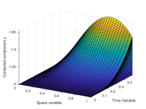
(a) Approximation to $y$

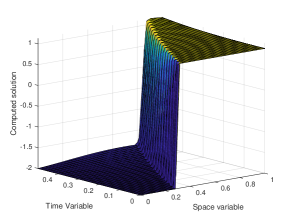
(b) Approximation to $u$

Figure 1: Example 1: Numerical approximations to $y$ and $u$ with $\varepsilon=2^{-12}$ and $N=M=64$

Table 1: Example 1: Maximum two-mesh global differences and orders of convergence for the function $y$

	N=M=32	N=M=64	N=M=128	N=M=256	N=M=512	N=M=1024	N=M=2048
$\varepsilon=2^{0}$	3.495E-02	9.470E-03	3.704E-03	1.656E-03	8.105E-04	4.011E-04	1.995E-04
	1.884	1.354	1.161	1.031	1.015	1.007
$\varepsilon=2^{-2}$	1.230E-02	5.783E-03	2.798E-03	1.376E-03	6.821E-04	3.396E-04	1.695E-04
	1.088	1.048	1.024	1.012	1.006	1.003
$\varepsilon=2^{-3}$	1.673E-02	1.079E-02	5.191E-03	2.547E-03	1.262E-03	6.280E-04	3.133E-04
	0.633	1.055	1.027	1.013	1.007	1.003
$\varepsilon=2^{-4}$	1.368E-02	7.991E-03	4.652E-03	2.642E-03	1.484E-03	8.235E-04	4.726E-04
	0.776	0.781	0.816	0.832	0.850	0.801
$\varepsilon=2^{-6}$	4.800E-03	2.698E-03	1.557E-03	8.862E-04	4.976E-04	2.763E-04	1.516E-04
	0.831	0.792	0.813	0.833	0.848	0.866
$\varepsilon=2^{-8}$	2.468E-03	1.323E-03	7.255E-04	3.993E-04	2.204E-04	1.221E-04	6.748E-05
	0.900	0.866	0.862	0.857	0.851	0.856
$\varepsilon=2^{-10}$	2.875E-03	1.679E-03	9.370E-04	5.184E-04	2.860E-04	1.572E-04	8.599E-05
	0.776	0.841	0.854	0.858	0.864	0.870
$\varepsilon=2^{-12}$	2.968E-03	1.707E-03	9.543E-04	5.288E-04	2.927E-04	1.612E-04	8.819E-05
	0.798	0.839	0.852	0.853	0.861	0.870
$\varepsilon=2^{-14}$	2.992E-03	1.714E-03	9.586E-04	5.313E-04	2.943E-04	1.623E-04	8.892E-05
	0.804	0.839	0.851	0.852	0.859	0.868
	⋮	⋮	⋮	⋮	⋮	⋮	⋮
$\varepsilon=2^{-26}$	3.001E-03	1.717E-03	9.600E-04	5.322E-04	2.949E-04	1.626E-04	8.913E-05
	0.806	0.839	0.851	0.852	0.859	0.867
$D^{N,M}$	3.495E-02	1.079E-02	5.191E-03	2.642E-03	1.484E-03	8.235E-04	4.726E-04
$P^{N,M}$	1.696	1.055	0.974	0.832	0.850	0.801

Example 2.

Consider the following test problem

$$\begin{array}[]{l}-\varepsilon u_{xx}+(1+t^{2})u_{x}+u+u_{t}=4x(1-x)t+t^{2},\quad(x,t)\in(0,1)\times(0,0.5],\\ u(x,0)=-x^{3},\ 0\leq x<0.3,\quad u(x,0)=(1-x)^{3},\ 0.3\leq x\leq 1,\\ u(0,t)=u(1,t)=0,\ 0<t\leq 0.5.\end{array}$$

The computed maximum two-mesh global differences and orders of convergence are given in Table 2. Unlike Example 1, the initial condition satisfies $[\phi^{\prime}](0.3)\neq 0$ and its influence on the orders of convergence is clearly shown in this table. The orders of convergence are reduced to a 0.5, which is in agreement with the error bound given in Theorem 1.

For this particular example, we show that more accurate approximations to the solution can be obtained if the decomposition given in Remark 3 is considered. The numerical approximation to $y_{1}$ and $u$ are displayed in Figure 3. The uniform two-mesh global differences and their orders of convergence are given in Table 3, showing that the numerical/analytical scheme converges globally and uniformly with almost first order when the component $y_{1}$ is approximated.

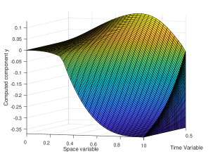
(a) Approximation to $y$

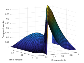
(b) Approximation to $u$

Figure 2: Example 2: Numerical approximations to $y$ and $u$ with $\varepsilon=2^{-12}$ and $N=M=64$

Table 2: Example 2: Maximum two-mesh global differences and orders of convergence for the function $y$

	N=M=32	N=M=64	N=M=128	N=M=256	N=M=512	N=M=1024	N=M=2048
$\varepsilon=2^{0}$	1.071E-02	1.000E-02	6.887E-03	5.201E-03	3.621E-03	2.685E-03	1.883E-03
	0.098	0.539	0.405	0.522	0.431	0.512
$\varepsilon=2^{-2}$	3.590E-03	4.569E-03	3.007E-03	2.481E-03	1.694E-03	1.314E-03	9.131E-04
	-0.348	0.603	0.278	0.550	0.367	0.525
$\varepsilon=2^{-4}$	7.415E-03	3.990E-03	2.255E-03	1.247E-03	7.917E-04	6.614E-04	4.582E-04
	0.894	0.823	0.854	0.656	0.259	0.530
$\varepsilon=2^{-6}$	1.125E-02	7.051E-03	4.061E-03	2.202E-03	1.154E-03	5.894E-04	2.964E-04
	0.674	0.796	0.883	0.933	0.969	0.992
$\varepsilon=2^{-8}$	1.425E-02	9.726E-03	6.373E-03	3.921E-03	2.277E-03	1.248E-03	6.590E-04
	0.551	0.610	0.701	0.784	0.867	0.922
$\varepsilon=2^{-10}$	1.519E-02	1.088E-02	7.564E-03	5.138E-03	3.344E-03	2.063E-03	1.198E-03
	0.482	0.524	0.558	0.620	0.697	0.784
$\varepsilon=2^{-12}$	1.543E-02	1.121E-02	7.945E-03	5.636E-03	3.911E-03	2.651E-03	1.725E-03
	0.461	0.497	0.495	0.527	0.561	0.620
$\varepsilon=2^{-14}$	1.550E-02	1.130E-02	8.048E-03	5.777E-03	4.102E-03	2.893E-03	2.007E-03
	0.456	0.490	0.478	0.494	0.504	0.528
	⋮	⋮	⋮	⋮	⋮	⋮	⋮
$\varepsilon=2^{-26}$	1.552E-02	1.133E-02	8.083E-03	5.827E-03	4.172E-03	2.989E-03	2.135E-03
	0.454	0.487	0.472	0.482	0.481	0.485
$D^{N,M}$	1.552E-02	1.133E-02	8.083E-03	5.827E-03	4.172E-03	2.989E-03	2.135E-03
$P^{N,M}$	0.454	0.487	0.472	0.482	0.481	0.485

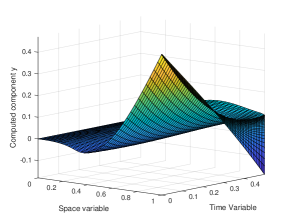
(a) Approximation to $y_{1}$

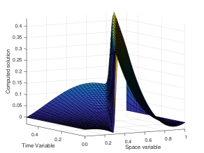
(b) Improved approximation to $u$

Figure 3: Example 2: Numerical approximation to $y_{1}$ and improved approximation to $u$ for $\varepsilon=2^{-12}$ and $N=M=64$

Table 3: Example 2: Uniform two-mesh global differences and orders of convergence for the function $y_{1}$

	N=M=32	N=M=64	N=M=128	N=M=256	N=M=512	N=M=1024	N=M=2048
$D^{N,M}$	1.403E-02	8.451E-03	4.856E-03	2.669E-03	1.413E-03	7.361E-04	3.789E-04
$P^{N,M}$	0.731	0.799	0.863	0.917	0.941	0.958

Example 3.

Consider the following test problem

$$\begin{array}[]{l}-\varepsilon u_{xx}+(1+t)u_{x}+u_{t}=4x(1-x)t+t^{2},\quad(x,t)\in(0,1)\times(0,2],\\ u(x,0)=-2,0\leq x<0.3,\quad u(x,0)=1,\ 0.3\leq x\leq 1,\\ u(0,t)=-2,\quad u(1,t)=1,\ 0<t\leq 2.\end{array}$$

The initial condition is discontinuous at $d=0.3$, $[\phi^{\prime}](0.3)=0$ and the characteristic curve $\Gamma^{*}$ is now given by $d(t)=t+t^{2}/2+0.3$. The final time has been chosen large enough so that the interior layer interacts with the boundary layer. Then, we use a piecewise uniform mesh in time (19) by computing $T^{*}$ with $d(T^{*})=1$. In this example, it is given by

$$T^{*}=\sqrt{1+2(1-d)}-1\approx 0.5492.$$

In Figure 4 a prominent layer near the boundary $x=1$ is observed for $t\geq T^{*}.$ Error bounds when the layers interact are discussed in § 3.2 and it is proved that Theorem 1 also applies. The maximum two-mesh global differences and the orders of convergence are given in Table 4 and it is observed that it is a uniformly and globally convergent scheme having almost first-order. All these numerical results agree with the error bound established in Theorem 1.

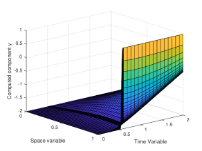
(a) Approximation to $y$

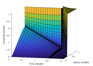
(b) Approximation to $u$

Figure 4: Example 3: Numerical approximations to $y$ and $u$ with $\varepsilon=2^{-12}$ and $N=M=64$

Table 4: Example 3: Maximum two-mesh global differences and orders of convergence for the function $y$

	N=M=32	N=M=64	N=M=128	N=M=256	N=M=512	N=M=1024	N=M=2048
$\varepsilon=2^{0}$	2.899E-02	3.735E-02	1.233E-02	4.263E-03	1.804E-03	8.821E-04	4.364E-04
	-0.365	1.599	1.532	1.241	1.032	1.015
$\varepsilon=2^{-2}$	4.847E-02	2.486E-02	1.259E-02	6.342E-03	3.182E-03	1.594E-03	7.977E-04
	0.963	0.981	0.990	0.995	0.997	0.999
$\varepsilon=2^{-3}$	7.498E-02	5.263E-02	2.677E-02	1.350E-02	6.782E-03	3.399E-03	1.702E-03
	0.511	0.975	0.988	0.993	0.996	0.998
$\varepsilon=2^{-4}$	7.313E-02	4.724E-02	2.811E-02	1.670E-02	9.579E-03	5.411E-03	3.145E-03
	0.630	0.749	0.751	0.802	0.824	0.783
$\varepsilon=2^{-6}$	7.543E-02	4.653E-02	2.755E-02	1.637E-02	9.407E-03	5.330E-03	2.973E-03
	0.697	0.756	0.751	0.799	0.820	0.842
$\varepsilon=2^{-8}$	7.872E-02	4.619E-02	2.731E-02	1.621E-02	9.305E-03	5.274E-03	2.942E-03
	0.769	0.758	0.753	0.801	0.819	0.842
$\varepsilon=2^{-10}$	7.993E-02	4.718E-02	2.746E-02	1.617E-02	9.282E-03	5.260E-03	2.934E-03
	0.761	0.781	0.764	0.801	0.819	0.842
$\varepsilon=2^{-12}$	7.996E-02	4.778E-02	2.797E-02	1.616E-02	9.278E-03	5.256E-03	2.932E-03
	0.743	0.772	0.791	0.801	0.820	0.842
$\varepsilon=2^{-14}$	8.020E-02	4.796E-02	2.821E-02	1.619E-02	9.278E-03	5.256E-03	2.932E-03
	0.742	0.765	0.801	0.804	0.820	0.842
	⋮	⋮	⋮	⋮	⋮	⋮	⋮
$\varepsilon=2^{-18}$	8.008E-02	4.806E-02	2.838E-02	1.632E-02	9.278E-03	5.255E-03	2.932E-03
	0.736	0.760	0.798	0.815	0.820	0.842
	⋮	⋮	⋮	⋮	⋮	⋮	⋮
$\varepsilon=2^{-26}$	7.995E-02	4.799E-02	2.836E-02	1.636E-02	9.293E-03	5.254E-03	2.931E-03
	0.736	0.759	0.794	0.816	0.823	0.842
$D^{N,M}$	8.020E-02	5.263E-02	2.838E-02	1.670E-02	9.579E-03	5.411E-03	3.145E-03
$P^{N,M}$	0.608	0.891	0.765	0.802	0.824	0.783

4.2 Extensions

Example 4.

Consider the following text problem

$$\begin{array}[]{l}-\varepsilon u_{xx}+(1+t^{2})u_{x}+u_{t}=4x(1-x)t+t^{2},\quad(x,t)\in(0,1)\times(0,0.5],\\ u(x,0)=-2x,0\leq x<d,\quad u(x,0)=1-x^{2},\ d\leq x\leq 1,\\ u(0,t)=4t^{2},\quad u(1,t)=t(t+0.5),\ 0<t\leq 0.5;\\ d:=\min\{0.3,\sqrt{\varepsilon}\}.\end{array}$$

In this example $[\phi](d)\neq 0,\ [\phi^{\prime}](d)\neq 0$, $d(t)=t+t^{3}/3+d$ and the interior and boundary layers do not merge (see Figure 5.) The aim of this test problem is to show numerically that the analytical/numerical method proposed in this paper can also be applied when the distance of the discontinuity point $(d,0)$ of the initial condition to the point $(0,0)$ depends on the singular perturbation parameter and $1>d\geq C\sqrt{\varepsilon}$. Note that the method will fail if $d=\varepsilon^{p},p>0.5$.

The numerical results in Table 5 suggest that the numerical approximations converge globally and uniformly with order 0.5. For other test examples with $d=O(\sqrt{\varepsilon})$ but $[\phi^{\prime}](d)=0$, we have observed numerically that the numerical approximations converge with almost first order. The proof of these observed orders of convergence for this problem class (with $d=O(\sqrt{\varepsilon})$) is an open question.

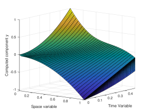
(a) Approximation to $y$

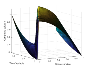
(b) Approximation to $u$

Figure 5: Example 4: Numerical approximations to $y$ and $u$ with $\varepsilon=2^{-12}$ and $N=M=64$

Table 5: Example 4: Maximum two-mesh global differences and orders of convergence for the function $y$

	N=M=32	N=M=64	N=M=128	N=M=256	N=M=512	N=M=1024	N=M=2048
$\varepsilon=2^{0}$	1.759E-02	1.215E-02	8.027E-03	6.110E-03	4.246E-03	3.134E-03	2.197E-03
	0.534	0.598	0.394	0.525	0.438	0.512
$\varepsilon=2^{-2}$	7.582E-03	5.363E-03	3.499E-03	2.916E-03	1.988E-03	1.534E-03	1.065E-03
	0.500	0.616	0.263	0.553	0.374	0.526
$\varepsilon=2^{-4}$	1.518E-02	7.788E-03	3.925E-03	2.172E-03	1.249E-03	7.257E-04	5.858E-04
	0.963	0.988	0.854	0.798	0.784	0.309
$\varepsilon=2^{-6}$	2.646E-02	1.492E-02	8.494E-03	4.779E-03	2.652E-03	1.455E-03	7.905E-04
	0.826	0.813	0.830	0.849	0.866	0.880
$\varepsilon=2^{-8}$	3.636E-02	1.969E-02	1.076E-02	5.774E-03	3.540E-03	2.057E-03	1.122E-03
	0.885	0.872	0.898	0.706	0.783	0.875
$\varepsilon=2^{-10}$	4.039E-02	2.084E-02	1.121E-02	5.998E-03	3.755E-03	2.668E-03	1.717E-03
	0.954	0.894	0.903	0.676	0.493	0.635
$\varepsilon=2^{-12}$	4.181E-02	2.112E-02	1.132E-02	6.059E-03	3.255E-03	2.252E-03	1.783E-03
	0.985	0.900	0.901	0.896	0.532	0.337
$\varepsilon=2^{-14}$	4.236E-02	2.121E-02	1.134E-02	6.073E-03	3.265E-03	1.753E-03	1.250E-03
	0.998	0.903	0.901	0.895	0.897	0.488
	⋮	⋮	⋮	⋮	⋮	⋮	⋮
$\varepsilon=2^{-26}$	4.281E-02	2.127E-02	1.135E-02	6.078E-03	3.268E-03	1.755E-03	9.405E-04
	1.009	0.906	0.901	0.895	0.897	0.900
$D^{N,M}$	4.281E-02	2.127E-02	1.135E-02	6.110E-03	4.246E-03	3.134E-03	2.197E-03
$P^{N,M}$	1.009	0.906	0.894	0.525	0.438	0.512

Example 5.

Finally, we consider the following test problem

$$\begin{array}[]{l}-\varepsilon u_{xx}+(1+x^{2})u_{x}+u_{t}=4x(1-x)t+t^{2},\quad(x,t)\in(0,1)\times(0,0.5],\\ u(x,0)=-2,0\leq x<0.1,\quad u(x,0)=1,\ 0.1\leq x\leq 1,\\ u(0,t)=-2,\quad u(1,t)=1,\ 0<t\leq 0.5.\end{array}$$

In this example $[\phi](0.1)=3\neq 0,\ [\phi^{\prime}](d)=0$ and the interior and boundary layers do not merge. Note that the convective coefficient depends on the space variable, while our error analysis assumes that $a=a(t).$ The characteristic curve $\Gamma^{*}$ is the solution of the initial value problem $d^{\prime}(t)=(1+d^{2}(t))$, with $d(0)=0.1$, which is given by $d(t)=(0.1+\tan t)/(1-0.1\tan t).$

In Table 6 we observe that the numerical method is not a parameter-uniform method when $a$ depends on the space variable. In order to design a uniformly convergent method in the case where $a=a(x,t)$, a more sophisticated scheme is required [5].

Table 6: Example 5: Maximum two-mesh global differences and orders of convergence for the function $y$

	N=M=32	N=M=64	N=M=128	N=M=256	N=M=512	N=M=1024	N=M=2048
$\varepsilon=2^{0}$	1.978E-01	6.835E-02	3.367E-02	4.361E-02	1.478E-02	4.979E-03	2.029E-03
	1.533	1.021	-0.373	1.561	1.570	1.295
$\varepsilon=2^{-2}$	2.811E-02	3.521E-02	1.235E-02	4.127E-03	1.802E-03	8.806E-04	4.355E-04
	-0.325	1.511	1.581	1.196	1.033	1.016
$\varepsilon=2^{-4}$	1.387E-02	6.663E-03	3.219E-03	1.529E-03	7.176E-04	3.341E-04	1.532E-04
	1.058	1.050	1.074	1.092	1.103	1.125
$\varepsilon=2^{-10}$	1.580E-01	9.484E-02	4.791E-02	2.418E-02	1.215E-02	6.088E-03	3.046E-03
	0.737	0.985	0.987	0.993	0.996	0.999
$\varepsilon=2^{-12}$	6.620E-01	2.759E-01	1.172E-01	5.656E-02	2.859E-02	1.431E-02	7.158E-03
	1.263	1.236	1.051	0.984	0.999	0.999
$\varepsilon=2^{-14}$	1.391E+00	6.782E-01	2.748E-01	1.113E-01	6.205E-02	3.102E-02	1.553E-02
	1.036	1.303	1.304	0.843	1.000	0.998
$\varepsilon=2^{-15}$	1.409E+00	7.023E-01	3.482E-01	1.451E-01	8.928E-02	4.509E-02	2.255E-02
	1.004	1.012	1.263	0.701	0.985	1.000
$\varepsilon=2^{-19}$	4.540E-03	2.705E-03	1.560E+00	4.250E-01	1.997E-01	2.022E-01	9.535E-02
	0.747	-9.171	1.876	1.089	-0.018	1.085
$\varepsilon=2^{-20}$	4.540E-03	2.705E-03	1.152E+00	4.582E-01	6.427E-01	3.221E-01	1.370E-01
	0.747	-8.734	1.330	-0.488	0.996	1.234
$\varepsilon=2^{-23}$	4.540E-03	2.705E-03	1.576E-03	9.104E-04	1.602E+00	8.004E-01	3.727E-01
	0.747	0.779	0.792	-10.781	1.001	1.103
$\varepsilon=2^{-26}$	4.540E-03	2.705E-03	1.576E-03	9.105E-04	5.055E-02	2.521E-02	1.559E+00
	0.747	0.779	0.792	-5.795	1.003	-5.950
$D^{N,M}$	1.409E+00	7.023E-01	1.560E+00	4.582E-01	1.602E+00	8.004E-01	1.559E+00
$P^{N,M}$	1.004	-1.151	1.767	-1.806	1.001	-0.961

5 Appendix: A set of singular functions

Below, we define a set of functions $\{\psi_{i}\}_{i=0}^{4}$ such that $L\psi_{i}=0$; $\psi_{i}\in C^{i-1+\gamma}(\bar{Q}),\ i\geq 1$ and each function $\psi_{i}$ is smooth within the open region $Q\setminus\Gamma^{*}$.

Define the two singular functions (see [1, (10)])

$$\psi_{0}(x,t):=\operatorname{erfc}\left(\frac{d(t)-x}{2\sqrt{\varepsilon t}}\right),\quad E(x,t):=e^{-\frac{(x-d(t))^{2}}{4\varepsilon t}}.$$ (20)

Then we explicitly write out the derivatives of these two functions

$$\frac{\partial\psi_{0}}{\partial x} = \frac{1}{\sqrt{\varepsilon\pi t}}E,\quad\frac{\partial E}{\partial x}=\frac{d(t)-x}{2\varepsilon t}E,$$

$$\varepsilon\frac{\partial^{2}\psi_{0}}{\partial x^{2}} = \frac{d(t)-x}{2t\sqrt{\varepsilon\pi t}}E,\quad\varepsilon\frac{\partial^{2}E}{\partial x^{2}}=\Bigl{(}\frac{(d(t)-x)^{2}}{2\varepsilon t}-1\Bigr{)}\frac{E}{2t},$$

$$\frac{\partial\psi_{0}}{\partial t} = \frac{1}{\sqrt{\varepsilon\pi t}}\Bigl{(}\frac{(d(t)-x)-2ta}{2t}\Bigr{)}E,$$

$$\frac{\partial E}{\partial t} = \frac{(d(t)-x)}{2\varepsilon t}\Bigl{(}\frac{(d(t)-x)}{2t}-a(t)\Bigr{)}E=\frac{\sqrt{\pi}(d(t)-x)}{2\sqrt{\varepsilon t}}\frac{\partial\psi_{0}}{\partial t}.$$

Hence, $L\psi_{0}=0.$ We define the continuous function

$$\psi_{1}(x,t):=(d(t)-x)\psi_{0}-2\frac{\sqrt{\varepsilon t}}{\sqrt{\pi}}E,$$ (21)

with

$$\frac{\partial\psi_{1}}{\partial t}=a(t)\psi_{0}-\frac{\sqrt{\varepsilon}}{\sqrt{\pi t}}E;\quad\frac{\partial\psi_{1}}{\partial x}=-\psi_{0}\quad\hbox{so that}\quad L\psi_{1}\equiv 0.$$

We now define the remaining functions:

$$\psi_{i}:=(d(t)-x)\psi_{i-1}+2\varepsilon t(i-1)\psi_{i-2},\qquad i=2,3,4;$$ (22)

and we can check that for $i=1,2,3,4$

$$\frac{\partial\psi_{i}}{\partial x}=-i\psi_{i-1},\ L\psi_{i}=0\quad\hbox{and}\quad\psi_{i}\in C^{i-1+\gamma}(\bar{Q)}.$$

Either side of $x=d$, we have the Taylor expansions for the initial condition

$$\phi(x)=\sum_{i=0}^{4}\phi^{(i)}(d^{*})\frac{(x-d)^{i}}{i!}+R_{0}(x),\quad d^{*}=\Bigl{\{}\begin{array}[]{ll}d^{-}\quad\hbox{ if }x<d\\ d^{+}\quad\hbox{ if }x>d\end{array};$$

with $R_{0}(x)\in C^{4}(0,1)$. Hence, we present the following expansion

$$u(x,t)=0.5\sum_{i=0}^{4}[\phi^{(i)}](d)\frac{(-1)^{i}}{i!}\psi_{i}(x,t)+R(x,t).$$ (23)

Note that for $i=1,2,3,4$

$$\frac{\partial^{i}\psi_{i}}{\partial x^{i}}=(-1)^{i}i!\psi_{0}\quad\hbox{and}\quad[\psi_{0}](d)=2,$$

which implies that $[u^{(i)}](d,0)=[\phi^{(i)}](d)$.

Define the paramaterized exponential function

$$E_{\gamma}(x,t):=e^{-\frac{\gamma(x-d(t))^{2}}{4\varepsilon t}},\qquad 0<\gamma<1.$$

Using the inequality $\operatorname{erfc}(z)\leq Ce^{-z^{2}}\leq Ce^{\gamma^{2}/4}e^{-\gamma z},\forall z\geq 0$ it follows that

$$|\psi_{0}(x,t)|\leq C,$$ (24a)

$$\Bigl{|}\frac{\partial^{j}}{\partial t^{j}}\psi_{0}(x,t)\Bigr{|},\Bigl{|}\frac{\partial^{j}}{\partial t^{j}}E(x,t)\Bigr{|}\leq C\left(\frac{1}{t}+\frac{1}{\sqrt{\varepsilon t}}\right)^{j}E_{\gamma}(x,t);\quad j=1,2;$$ (24b)

$$\Bigl{|}\frac{\partial^{i}}{\partial x^{i}}\psi_{0}(x,t)\Bigr{|},\Bigl{|}\frac{\partial^{i}}{\partial x^{i}}E(x,t)\Bigr{|}\leq C\left(\frac{1}{\sqrt{\varepsilon t}}\right)^{i}E_{\gamma}(x,t),\ 1\leq i\leq 4;$$ (24c)

$$\Bigl{|}\frac{\partial}{\partial t}\psi_{1}(x,t)\Bigr{|}\leq C\left(1+\sqrt{\frac{\varepsilon}{t}}\right)E(x,t)+C,$$ (24d)

$$\Bigl{|}\frac{\partial^{2}}{\partial t^{2}}\psi_{1}(x,t)\Bigr{|}\leq C\left(\frac{1}{t}+\frac{1}{t}\sqrt{\frac{\varepsilon}{t}}+\frac{1}{\sqrt{\varepsilon t}}\right)E_{\gamma}(x,t)+C,$$ (24e)

$$|\psi_{1}(x,t)|\leq C,\,\,\Bigl{|}\frac{\partial^{i}}{\partial x^{i}}\psi_{1}(x,t)\Bigr{|}\leq C\left(\frac{1}{\sqrt{\varepsilon t}}\right)^{i-1}E_{\gamma}(x,t),\,1\leq i\leq 4.$$ (24f)

For the next terms, we can also establish the bounds

$$\Bigl{|}\frac{\partial}{\partial t}\psi_{2}(x,t)\Bigr{|}\leq C,\quad\Bigl{|}\frac{\partial^{2}}{\partial x^{2}}\psi_{2}(x,t)\Bigr{|}\leq C;$$ (25a)

on the second time derivatives

$$\Bigl{|}\frac{\partial^{2}}{\partial t^{2}}\psi_{2}(x,t)\Bigr{|} \leq C\varepsilon\left(\frac{1}{t}+\frac{1}{\sqrt{\varepsilon t}}+\frac{1}{\varepsilon}\right)E_{\gamma}(x,t)+C$$

$$\leq C\left(1+\frac{\varepsilon}{t}\right)E_{\gamma}(x,t)+C,$$ (25b)

$$\Bigl{|}\frac{\partial^{2}}{\partial t^{2}}\psi_{3}(x,t)\Bigr{|} \leq C\sqrt{\varepsilon t}\left(1+\frac{\varepsilon}{t}\right)E_{\gamma}(x,t)+C,$$ (25c)

$$\Bigl{|}\frac{\partial^{2}}{\partial t^{2}}\psi_{4}(x,t)\Bigr{|} \leq C\varepsilon E_{\gamma}(x,t)+C$$ (25d)

on the fourth space derivatives

$$\Bigl{|}\frac{\partial^{4}}{\partial x^{4}}\psi_{j}(x,t)\Bigr{|}\leq C(\sqrt{\varepsilon t})^{j-4}E_{\gamma}(x,t)+C,\quad j=2,3,4$$ (25e)

and on the third space derivatives

$$\Bigl{|}\frac{\partial^{3}}{\partial x^{3}}\psi_{2}(x,t)\Bigr{|}\leq C\frac{1}{\sqrt{\varepsilon t}}E_{\gamma}(x,t)+C,\quad\Bigl{|}\frac{\partial^{3}}{\partial x^{3}}\psi_{3}(x,t)\Bigr{|},\Bigl{|}\frac{\partial^{3}}{\partial x^{3}}\psi_{4}(x,t)\Bigr{|}\leq C.$$ (25f)

References

- [1] L. Bobisud, Parabolic equations with a small parameter and discontinuous data, J. Math. Anal. Appl., v. 26, (1969), 208–220.
- [2] P.A. Farrell, A.F. Hegarty, J.J.H. Miller, E. O’Riordan and G.I. Shishkin, Robust computational techniques for boundary layers, CRC Press, 2000.
- [3] A. Friedman, Partial differential equations of parabolic type, Prentice-Hall, Englewood Cliffs, N.J., 1964.
- [4] J.L. Gracia and E. O’Riordan, A singularly perturbed convection–diffusion problem with a moving interior layer, Int. J. Num. Anal. Mod., v. 9 (4), (2012), 823–843.
- [5] J.L. Gracia and E. O’Riordan, Parameter-uniform approximations for a singularly perturbed convection-diffusion problems with a discontinuous initial condition, Arxiv.
- [6] J.L. Gracia and E. O’Riordan, Numerical approximation of solution derivatives of singularly perturbed parabolic problems of convection–diffusion type, Math. Comput., v. 85, (2016), 581–599.
- [7] J.L. Gracia and E. O’Riordan, Singularly perturbed reaction-diffusion problems with discontinuities in the initial and/or the boundary data, J. Comput. Appl. Math., v. 370, (2020), 112638, 17pp.
- [8] J.J.H. Miller, E. O’Riordan and G.I. Shishkin and L.P. Shishkina, Fitted mesh methods for problems with parabolic boundary layers, Mathematical Proceedings of the Royal Irish Academy, v. 98A, (1998), 173–190.
- [9] G.I. Shishkin, Grid approximation of singularly perturbed parabolic convection-diffusion equations with a piecewise-smooth initial condition, Zh. Vychisl. Mat. Mat. Fiz., v. 46 (1), (2006), 52–76.
- [10] G. I. Shishkin, Discrete approximations of singularly perturbed elliptic and parabolic equations, Russ. Akad. Nauk, Ural Section, Ekaterinburg, 1992 (in Russian).
- [11] M. Stynes and E. O’Riordan, A uniformly convergent Galerkin method on a Shishkin mesh for a convection-diffusion problem, J. Math. Anal. Appl., v. 214, (1997), 36–54.
- [12] U.Kh. Zhemukhov, Parameter-uniform error estimate for the implicit four-point scheme for a singularly perturbed heat equation with corner singularities, Translation of Differ. Uravn. v. 50 (7) (2014), v. 7, 923–936; Differ. Equ. v. 50 (7), (2014), 913–926.