Asynchronous Optimization over Graphs: Linear Convergence under Error Bound Conditions

Abstract

We consider convex and nonconvex constrained optimization with a partially separable objective function: agents minimize the sum of local objective functions, each of which is known only by the associated agent and depends on the variables of that agent and those of a few others. This partitioned setting arises in several applications of practical interest. We propose what is, to the best of our knowledge, the first distributed, asynchronous algorithm with rate guarantees for this class of problems. When the objective function is nonconvex, the algorithm provably converges to a stationary solution at a sublinear rate whereas linear rate is achieved under the renowned Luo-Tseng error bound condition (which is less stringent than strong convexity). Numerical results on matrix completion and LASSO problems show the effectiveness of our method.

I Introduction

We study distributed, nonsmooth, nonconvex optimization with a partially separable sum-cost function. Specifically, consider a set of $N$ agents, each of them controlling/updating a subset of the $n$ variables $\mathbf{x}\in\mathbb{R}^{n}$. Partitioning $\mathbf{x}=(\mathbf{x}_{1}^{T},\ldots,\mathbf{x}_{N}^{T})^{T}$, $\mathbf{x}_{i}\in\mathbb{R}^{n_{i}}$ is the block of variables owned by agent $i\in\mathcal{N}\triangleq\{1,\ldots,N\}$, with $\sum_{i}n_{i}=n$. All agents cooperatively aim at solving the following problem:

$$\begin{array}[]{rl}\underset{\mathbf{x}_{i}\in\mathcal{X}_{i},i\in\mathcal{N}}{\min}&V(\mathbf{x})\triangleq\underbrace{\sum\limits_{i=1}^{N}f_{i}(\mathbf{x}_{\mathcal{N}_{i}})}_{\triangleq F(\mathbf{x})}+\underbrace{\sum\limits_{i=1}^{N}g_{i}(\mathbf{x}_{i})}_{\triangleq G(\mathbf{x})},\end{array}$$ (P)

where $\mathcal{N}_{i}$ denotes a small subset of $\mathcal{N}$ including the index $i$ and $\mathbf{x}_{\mathcal{N}_{i}}\triangleq[\mathbf{x}_{j}]_{j\in\mathcal{N}_{i}}$ denotes the column vector containing the blocks of $\mathbf{x}$ indexed by $\mathcal{N}_{i}$; $\mathcal{X}_{i}\subseteq\mathbb{R}^{n_{i}}$ is a closed convex set; $f_{i}$ is a smooth (nonconvex) function that depends only on $\mathbf{x}_{\mathcal{N}_{i}}$; and $g_{i}$ is a convex (nonsmooth) function, instrumental to encode structural constraints on the solution, such as sparsity. Both $f_{i}$ and $g_{i}$ are assumed to be known only by agent $i$.

The above formulation is motivated by a variety of applications of practical interest. For instance, loss functions arising from many machine learning problems have the “sparse” pattern of $V$ in (P): $n$ and $N$ are both very large but each $f_{i}$ depends only on a small number of components of $\mathbf{x}$, i.e., each subvector $\mathbf{x}_{\mathcal{N}_{i}}$ contains just a few components of $\mathbf{x}$. The same partitioned structure in (P) is suitable also to model networked systems wherein agents are connected through a physical communication network and can communicate only with their immediate neighbors. In this setting, often $\mathcal{N}_{i}$ represents the set of neighbors of agent $i$ (including agent $i$ itself). Examples of such applications include resource allocation problems and network utility maximization [1], state estimation in power networks [2], cooperative localization in wireless networks [3], and map building in robotic networks. Some concrete instances of Problem (P) are discussed in Sec. II.

I-A Major contributions

We focus on the design of distributed, asynchronous algorithms for (P), in the following sense: i) Agents can update their block-variables at any time, without any coordination; and ii) when updating their own variables, agents can use a delayed out-of-sync information from the others. No constraint is imposed on the delay profiles: delays can be arbitrary, possibly time-varying (but bounded). This model captures several forms of asynchrony: some agents execute more iterations than others; some agents communicate more frequently than others; and inter-agent communications can be unreliable and/or subject to unpredictable, unknown, time-varying delays.

While several forms of asynchrony have been studied in the literature–see Sec. I-B for an overview of most relevant results–we are not aware of any distributed scheme that is compliant to the asynchronous model (i)-(ii) and tailored to the partitioned (nonconvex) distributed formulation (P). This paper fills this gap and proposes a general distributed, asynchronous algorithmic framework for convex and nonconvex instances of (P). The algorithm builds on Successive Convex Approximation (SCA) techniques: agents solve asynchronously [in the sense (i) and (ii) above] strongly convex approximations of the original problem (P) by using (possibly) outdated information on the variables and the gradients of the other agents. No specific activation mechanism for the agents’ updates, coordination, or communication protocol is assumed, but only some mild conditions ensuring that information used in the updates does not become infinitely old. For nonconvex instances of $V$, we prove that i) every limit point of the sequence generated by the proposed asynchronous algorithm is a stationary solution of (P); and ii) a suitable measure of stationarity vanishes at a sublinear rate. When $V$ further satisfies the Luo-Tseng error bound condition [4, 5], both the sequence and the objective value converge at an R-linear rate (when $V$ is nonconvex, convergence is to stationary solutions). This error bound condition is weaker than strong convexity and it is satisfied by a variety of problems of interest, such as LASSO, Group LASSO, and Logistic Regression, just to name a few (cf. Sec. III-A). While linear convergence under error bounds has been proved for many centralized algorithms [4, 6, 7, 8, 9], we are not aware of any such a result in the distributed setting; current works require strong convexity to establish linear rate of synchronous and asynchronous distributed algorithms (see, e.g., [10, 11, 12] and references therein). As a byproduct, our results provide also a positive answer to the open question whether linear convergence could be proved for distributed asynchronous algorithms solving highly dimensional empirical risk minimization problems, such as LASSO and Logistic Regression, a fact that was empirically observed but, to our knowledge, never proved.

I-B Related Works

Since the seminal work [13], asynchronous parallelism has been applied to several centralized solution methods, including (randomized) block-coordinate descent schemes [6, 13, 14, 15, 16, 17], and stochastic gradient algorithms [18, 19]. However, those methods are not applicable to Problem (P), since they would require each agent to know the entire objective function $V$.

Distributed schemes exploring (some form of) asynchrony have been studied in [20, 21, 22, 23, 24, 25, 26, 27, 28, 29, 30, 31, 32, 33, 34, 35, 36, 37, 38, 39]; next, we group them based upon the asynchrony features (i) and (ii).

(a) Random activation and no delays [20, 21, 22, 23, 24, 25, 26, 27, 40]: While substantially different in the form of the updates performed by the agents, these schemes are all asynchronous in the sense of feature (i) only. Agents (or edge-connected agents) are randomly activated but, when performing their computations/updates, they must use the current information from their neighbors. This means that no form of delay is allowed. Furthermore, between two activations, agents must be in idle mode (i.e., able to continuously receive information). Some form of coordination is thus needed to enforce the above conditions. All the schemes in this group but [26] can deal with convex objectives only; and none of the above works provide a convergence rate or complexity analysis.

(b) Synchronous activation and delays [28, 29, 30, 31, 32, 33]: These schemes consider synchronous activation/updates of the agents, which can tolerate fixed computation delays (e.g., outdated gradient information) [28, 29] or fixed [30, 33] or time-varying [31, 32] communication delays. However delays cannot be arbitrary, but must be such that no loss can ever occur in the network: every agent’s message must reach its intended destination within a finite time interval. Finally, all these algorithms are applicable only to convex problems.

(c) Random/cyclic activations and some form of delay [34, 35, 36, 37, 38, 39, 41, 42, 43, 44]: These schemes allow for random [34, 35, 37, 36, 41] or deterministic uncoordinated [38, 39, 42, 43, 45, 44] activation of the (edge-based) agents, together with the presence of some form of delay in the updates/computations. Specifically, [34, 35, 38] can handle link failures–the information sent by an agent to its neighbors either gets lost or received with no delay–but cannot deal with other forms of delay (e.g., communication delays). In [37, 36, 41] a probabilistic model is assumed whereby agents are randomly activated and update their local variables using possibly delayed information. The model requires that the random variables modeling the activation of the agents are i.i.d and independent of the delay vector used by the agent to perform its update. While this assumption makes the convergence analysis possible, in reality there is a strong dependence of the delays on the activation index, as also noted by the same authors [37, 36]; see [15] for a detailed discussion on this issue and some counter examples. Closer to our setting are the asynchronous methods in [39, 36, 10, 42, 43, 45, 44]. These models however assume that each function $f_{i}$ depends on the entire vector $\mathbf{x}$. As a consequence, a consensus mechanism on all the optimization variables is employed among the agents at each iteration. Because of that, a direct application of these consensus-based algorithms to the partitioned formulation (P) would lead to very inefficient schemes calling for unnecessary computation and communication overheads. Furthermore, the ADMM-like schemes [41, 42, 43, 45, 44, 39] can be implemented only on very specific network architectures, such as star networks or hierarchical topologies with multiple master and worker nodes. Finally, notice that, with the exception of [35, 39, 10, 41, 42, 43, 45, 44] (resp. [38]), all these schemes are applicable to convex problems (resp. undirected graphs) only, with [34] further assuming that all the functions $f_{i}$ have the same minimizer.

The rest of the paper is organized as follows: Section II discusses some motivating applications. The proposed algorithm is introduced and analyzed in Section III. Finally, numerical results are presented in Section IV.

II Motivating Examples

We discuss next two instances of Problem (P), which will be also used in our numerical experiments to test our algorithms (cf. Sec. IV). The first case study is the matrix completion problem–an example of large-scale nonconvex empirical risk minimization. We show how to exploit the sparsity pattern in the data to rewrite the problem in the form (P), so that efficient asynchronous algorithms levering multi-core architectures can be developed. The second example deals with learning problems from networked data sets; in this setting data are distributed across multiple nodes, whose communication network is modeled as a (directed) graph.
Example #1 –Matrix completion: The matrix completion problem consists of estimating a low-rank matrix $\mathbf{Z}\in\mathbb{R}^{M\times N}$ from a subset $\Omega\subseteq\{1,\ldots,M\}\times\{1,\ldots,N\}$ of its entries. Postulating the low-rank factorization $\mathbf{Z}=\mathbf{X}^{T}\mathbf{Y}$, with $\mathbf{X}\in\mathbb{R}^{r\times M}$ and $\mathbf{Y}\in\mathbb{R}^{r\times N}$, the optimization problem reads [46]:

$$\underset{\overset{\scriptstyle\mathbf{X}\in\mathbb{R}^{r\times M}}{\scriptstyle\mathbf{Y}\in\mathbb{R}^{r\times N}}}{\min}\;V(\mathbf{X},\mathbf{Y})\triangleq\frac{1}{2}\left\|(\mathbf{X}^{T}\mathbf{Y}-\mathbf{Z})_{\Omega}\right\|_{F}^{2}+\frac{\lambda}{2}\left\|\mathbf{X}\right\|_{F}^{2}+\frac{\xi}{2}\left\|\mathbf{Y}\right\|_{F}^{2},\vspace{-0.1cm}$$ (1)

where $\|\cdot\|_{F}$ is the Frobenius norm; $(\cdot)_{\Omega}$ is the projection operator, defined as $[(\mathbf{X})_{\Omega}]_{(i,j)}=\mathbf{X}_{(i,j)}$, if $(i,j)\in\Omega$; and $[(\mathbf{X})_{\Omega}]_{(i,j)}=0$ otherwise; and $\lambda,\xi>0$ are regularization parameters. In many applications, the amount of data is so large that storage and processing from a single agent (e.g., core, machine) is not efficient or even feasible. The proposed approach is then to leverage multi-core machines by first casting (1) in the form (P), and then employing the parallel asynchronous framework developed in this paper.

Consider a distributed environment composed of $N$ agents, and assume that the known entries $z_{mn}$, $(m,n)\in\Omega$, are partitioned among the agents. This partition along with the sparsity pattern of $(\mathbf{Z})_{\Omega}$ induce naturally the following splitting of the optimization variables $\mathbf{X}$ and $\mathbf{Y}$ across the agents. Let $\mathbf{x}_{m}$ and $\mathbf{y}_{n}$ denote the $m$-th and the $n$-th column of $\mathbf{X}$ and $\mathbf{Y}$, respectively; the agent owning $z_{mn}$ will control/update the variables $\mathbf{x}_{m}$ (or $\mathbf{y}_{n}$), and it is connected to the agent that optimizes the column $\mathbf{y}_{n}$ (or $\mathbf{x}_{m}$). By doing so, we minimize the overlapping across the block-variables and, consequently, the communications among the agents. Problem (1) can be then rewritten in the multi-agent form (P), setting

$$f_{i}((\mathbf{X},\mathbf{Y})_{\mathcal{N}_{i}})=\frac{1}{2}\,\sum\limits_{(m,n)\in\Omega_{i}}(\mathbf{x}_{m}^{T}\,\mathbf{y}_{n}-z_{mn})^{2}\vspace{-0.3cm}$$ (2)

and

$$g_{i}\left(\{\mathbf{x}_{m}\}_{m\in X_{i}},\{\mathbf{y}_{n}\}_{n\in Y_{i}}\right)=\frac{\lambda}{2}\sum\limits_{m\in X_{i}}\|\mathbf{x}_{m}\|^{2}_{2}+\frac{\xi}{2}\sum\limits_{n\in Y_{i}}\|\mathbf{y}_{n}\|_{2}^{2},$$ (3)

where $\Omega_{i}\subseteq\Omega$ contains the indices associated to the components of $(\mathbf{Z})_{\Omega}$ owned by agent $i$, and $X_{i}$ (resp. $Y_{i}$) is the set of the column indexes of $\mathbf{X}$ (resp. $\mathbf{Y}$) controlled by agent $i$.

Example #2 – Empirical risk minimization over networks: Consider now a network setting where data are distributed across $N$ geographically separated nodes. As concrete example, let us pick the renowned LASSO problem [47]:

$$\begin{array}[]{rl}\underset{\mathbf{x}=(\mathbf{x}_{1}^{T},\ldots,\mathbf{x}^{T}_{N})^{T}\in\mathbb{R}^{n}}{\min}&\|\mathbf{Ax}-\mathbf{b}\|_{2}^{2}+\lambda\|\mathbf{x}\|_{1},\end{array}$$ (4)

where $\mathbf{A}\in\mathbb{R}^{m\times n},\mathbf{b}\in\mathbb{R}^{m}$, and $\lambda>0$ is a regularization parameter. Note that (4) easily falls into Problem (P); for each $i\in\mathcal{N}$, it is sufficient to set $f_{i}(\mathbf{x})=\|\mathbf{A}_{i}\mathbf{x}+\mathbf{b}_{i}\|_{2}^{2}$, with $\mathbf{A}_{i}\in\mathbb{R}^{m\times n}$ and $\mathbf{b}_{i}\in\mathbb{R}^{m}$ such that $\mathbf{A}=\sum_{i=1}^{N}\mathbf{A}_{i}$ and $\mathbf{b}=\sum_{i=1}^{N}\mathbf{b}_{i}$; and $g_{i}=\|\mathbf{x}_{i}\|_{1}$. $\mathbf{A}_{i}$ and $\mathbf{b}_{i}$ represent in fact the data stored at agent $i$’s side. Under specific sparsity patterns in the data, the local matrices $\mathbf{A}_{i}$ may be (or constructed to be) such that each local function $f_{i}$ depends only on some of the block variables $\mathbf{x}_{i}$. These dependencies will define the sets $\mathcal{N}_{i}$ associated to each agent $i$. Note that $\mathcal{N}_{i}$ need not coincide with the neighbors of agent $i$ in the communication network (graph). That is, the graph modeling the dependence across the block-variables–the one with node set $\mathcal{N}$ and edge set $\mathcal{E}=\{(i,j):j\in\mathcal{N}_{i},\text{for some}\,i\!\in\!\mathcal{N}\}$–might not coincide with the communication graph. This can be desirable, e.g., when the communication graph is populated by inefficient communication links, which one wants to avoid using.

III Distributed Asynchronous Algorithm

In the proposed asynchronous model, agents update their block-variables without any coordination. Let $k$ be the iteration counter: the iteration $k\rightarrow k+1$ is triggered when one agent, say $i$, updates its own block $\mathbf{x}_{i}$ from $\mathbf{x}_{i}^{k}$ to $\mathbf{x}_{i}^{k+1}$. Hence, $\mathbf{x}^{k}$ and $\mathbf{x}^{k+1}$ only differ in the $i$-th block $\mathbf{x}_{i}$. To perform its update, agent $i$ minimizes a strongly convex approximation of $\sum_{j\in\mathcal{N}_{i}}f_{j}-$the part of $V$ that depends on $\mathbf{x}_{i}-$using possibly outdated information collected from the other agents $j\in\mathcal{N}_{i}$. To represent this situation, let $\mathbf{x}_{j}^{k-d_{j}^{k}(i,i)}$, $j\in\mathcal{N}_{i}\backslash\{i\}$, denote the estimate held by agent $i$ of agent $j$’s variable $\mathbf{x}_{j}^{k}$, where $d^{k}_{j}(i,i)$ is a nonnegative (integer) delay (the reason for the double index $(i,i)$ in $d^{k}_{j}$ will become clear shortly). If $d^{k}_{j}(i,i)=0$, agent $i$ owns the most recent information on the variable of agent $j$, otherwise $\mathbf{x}_{j}^{k-d^{k}_{j}(i,i)}$ is some delayed version of $\mathbf{x}_{j}^{k}$. We define as $\mathbf{d}^{k}(i,i)\triangleq[d_{l}^{k}(i,i)]_{l\in\mathcal{N}_{i}}$ the delay vector collecting these delays; for ease of notation $\mathbf{d}^{k}(i,i)$ contains also the value $d^{k}_{i}(i,i)$, set to zero, as each agent has always access to current values of its own variables. Using the above notation and recalling that $f_{i}$ depends on $\mathbf{x}_{\mathcal{N}_{i}}$, agent $i$ at iteration $k$ solves the following strongly convex subproblem:

$${\widehat{\mathbf{x}}_{i}^{k}\!\triangleq\underset{\mathbf{x}_{i}\in\mathcal{X}_{i}}{\arg\min}\,\Bigg{\{}\tilde{f}_{i}\left(\mathbf{x}_{i};\mathbf{x}_{\mathcal{N}_{i}}^{k-\mathbf{d}^{k}(i,i)}\right)+}$$ (5)

$$\sum\limits_{j\in\mathcal{N}_{i}\backslash\{i\}}\!\!\!\!\left\langle\nabla_{\mathbf{x}_{i}}f_{j}\left(\mathbf{x}_{\mathcal{N}_{j}}^{k-\mathbf{d}^{k}(i,j)}\right),\mathbf{x}_{i}\!-\!\mathbf{x}_{i}^{k}\right\rangle+g_{i}(\mathbf{x}_{i})\Bigg{\}},$$

where we defined $\mathbf{x}_{\mathcal{N}_{j}}^{k-\mathbf{d}^{k}(i,j)}\triangleq[\mathbf{x}_{l}^{k-d^{k}_{l}(i,j)}]_{l\in\mathcal{N}_{j}}$, $j\in\mathcal{N}_{i}$.

The term $\tilde{f}_{i}$ in (5) is a strongly convex surrogate that replaces the nonconvex function $f_{i}$ known by agent $i$; an outdated value of the variables of the other agents is used, $\mathbf{x}_{\mathcal{N}_{i}}^{k-\mathbf{d}^{k}(i,i)}$, to build this function. Examples of valid surrogates are discussed in Sec. III-A. The second term in (5) approximates $\sum_{j\in\mathcal{N}_{i}\backslash\{i\}}f_{j}$ by replacing each $f_{j}$ by its first order approximation at (possibly outdated) $\mathbf{x}_{\mathcal{N}_{j}}^{k-\mathbf{d}^{k}(i,j)}$ (with $\nabla_{\mathbf{x}_{i}}f_{j}$ denoting the gradient of $f_{j}$ with respect to the block $\mathbf{x}_{i}$), where $\mathbf{d}^{k}(i,j)\triangleq\left[d^{k}_{l}(i,j)\right]_{l\in\mathcal{N}_{j}}$, with $d_{l}^{k}(i,j)\geq 0$ representing the delay of the information that $i$ knows about the gradient $\nabla_{\mathbf{x}_{i}}f_{j}$. This source of delay on the gradients is due to two facts, namely: i) agents $j\in\mathcal{N}_{i}\setminus\{i\}$ may communicate to $i$ its gradient $\nabla_{\mathbf{x}_{i}}f_{j}$ occasionally; and ii) $\nabla_{\mathbf{x}_{i}}f_{j}$ is generally computed at some outdated point, as agent $j$ itself may not have access of the last information of the variables of the agents in $\mathcal{N}_{j}\setminus\{j\}$.

Once ${\widehat{\mathbf{x}}_{i}^{k}}$ has been computed, agent $i$ sets

$$\mathbf{x}_{i}^{k+1}=\mathbf{x}^{k}_{i}+\gamma\left({\widehat{\mathbf{x}}_{i}^{k}}-\mathbf{x}_{i}^{k}\right),$$ (6)

where $\gamma\in(0;1]$ is suitably chosen stepsize (cf. Sec. III-A).

The proposed distributed asynchronous algorithm, termed Distributed Asynchronous FLexible ParallEl Algorithm (DAsyFLEXA), is formally described in Algorithm 1. We set $\mathbf{x}^{t}_{i}=\mathbf{x}^{0}_{i}$, for all $t<0$ and $i\in\mathcal{N}$, without loss of generality.

Algorithm 1 Distributed Asynchronous FLexible ParallEl Algorithm (DAsyFLEXA)

  Initialization: $k=0$; $\mathbf{x}^{0}\in\mathcal{X}\triangleq\prod_{i}\mathcal{X}_{i}$; $\mathbf{x}^{t}=\mathbf{x}^{0}$, $t<0$; $\gamma\in(0;1]$.

  while  a termination criterion is not met do

     (S.1): Pick agent $i^{k}$ and delays $\{\mathbf{d}^{k}(i^{k},j)\}_{j\in\mathcal{N}_{i^{k}}}$;

     (S.2): Compute $\widehat{\mathbf{x}}_{i^{k}}^{k}$ according to (5);

     (S.3): Update $\mathbf{x}_{i^{k}}^{k}$ according to (6);

     (S.4): Update the global iteration counter $k\leftarrow k+1$;

  end while

We stress that agents need know neither the iteration counter $k$ nor the vector of delays. No one “picks agent $i^{k}$ and the delays $\{\mathbf{d}^{k}(i^{k},j)\}_{j\in\mathcal{N}_{i^{k}}}$” in (S.1). This is just an a posteriori view of the algorithm dynamics: all agents asynchronously and continuously collect information from their neighbors and use it to update $\mathbf{x}_{i}$; when one agent has completed an update the iteration index $k$ is increased and $i^{k}$ is defined.

III-A Assumptions

Before studying convergence of Algorithm 1, we state the main assumptions on Problem (P) and the algorithmic choices.

On Problem (P). Below, we will use the following conventions: When a function is said to be differentiable on a certain domain, it is understood that the function is differentiable on an open set containing the domain. We say that $f_{i}$ is block-$LC^{1}$ on a set if it is continuously differentiable on that set and $\nabla_{\mathbf{x}_{j}}f_{i}$ are locally Lipschitz. We say $V$ is coercive on $\mathcal{X}=\prod_{i}\mathcal{X}_{i}$, if $\lim\limits_{\begin{subarray}{c}\|\mathbf{x}\|\to+\infty,\mathbf{x}\in{\cal X}\end{subarray}}V(\mathbf{x})=+\infty$; this is equivalent to requiring that all level sets of $V$ in $\cal X$ are compact.

Assumption A (On Problem (P)):

(A1)

Each set $\mathcal{X}_{i}\subseteq\mathbb{R}^{n_{i}}$ is nonempty, closed, and convex;

(A2)

At least one of the following conditions is satisfied

(a) ${\cal L}^{0}\triangleq\{\mathbf{x}\in{\cal X}:V(\mathbf{x})\leq V(\mathbf{x}^{0})\}$ is compact and all $f_{i}$ are block-$LC^{1}$ on ${\mathcal{X}_{\mathcal{N}_{i}}\triangleq\underset{j\in\mathcal{N}_{i}}{\Pi}\mathcal{X}_{j}}$;

(b) All $f_{i}$ are $C^{1}$ and their gradients $\nabla_{\mathbf{x}_{j}}f_{i}$, $j\in{\cal N}_{i}$, are globally Lipschitz on $\mathcal{X}_{\mathcal{N}_{i}}$;

(A3)

Each $g_{i}:\mathcal{X}_{i}\rightarrow\mathbb{R}$ is convex;

(A4)

Problem (P) has a solution;

(A5)

The communication graph $\mathcal{G}$ is connected.

The above assumptions are standard and satisfied by many practical problems. For instance, A2(a) holds if $V$ is coercive on $\cal X$ and all $f_{i}$ are block-$LC^{1}$ on $\mathcal{X}_{\mathcal{N}_{i}}$. Note that Example #2 satisfies A2(b); A2(a) is motivated by applications such as Example #1, which do not satisfy A2(b). A3 is a common assumption in the literature of parallel and distributed methods for the class of problems (P); two renowned examples are $g_{i}(\mathbf{x}_{i})=\|\mathbf{x}_{i}\|_{1}$ and $g_{i}(\mathbf{x}_{i})=\|\mathbf{x}_{i}\|_{2}$. Finally, A4 is satisfied if, for example, $V$ is coercive or if $\cal X$ is bounded.

Remark 1.

Extensions to the case of directed graphs or the case where each agent updates multiple block-variables are easy, but not discussed here for the sake of simplicity.

The aim of Algorithm 1 is to find stationary solutions of (P), i.e. points $\mathbf{x}^{\star}\in\mathcal{X}$ such that

$$\left\langle\nabla F(\mathbf{x}^{\star})+\boldsymbol{\xi},\mathbf{y}-\mathbf{x}^{\star}\right\rangle+G(\mathbf{y})-G(\mathbf{x}^{\star})\geq 0,\qquad\forall\mathbf{y}\in\mathcal{X}.$$

Let $\mathcal{X}^{\star}\subseteq\mathbb{R}^{n}$ denote the set of such stationary solutions.

On an error bound condition. We prove linear convergence of Algorithm 1 under the Luo-Tseng error bound condition, which is stated next. Recall the definition: given $\alpha>0$,

$$\texttt{prox}_{\alpha G}(\mathbf{z})\triangleq\underset{\mathbf{y}\in\mathcal{X}}{\arg\min}\,\left\{\alpha G(\mathbf{y})+\frac{1}{2}\|\mathbf{y}-\mathbf{z}\|_{2}^{2}\right\}.$$

Furthermore, given $\mathbf{x}\in\mathbb{R}^{n}$, let

$$d(\mathbf{x},\mathcal{X}^{\star})\triangleq\underset{\mathbf{x}^{\star}\in\mathcal{X}^{\star}}{\min}\|\mathbf{x}-\mathbf{x}^{\star}\|_{2},\qquad P_{\mathcal{X}^{\star}}(\mathbf{x})\triangleq\underset{\mathbf{x}^{\star}\in\mathcal{X}^{\star}}{\text{argmin}}\|\mathbf{x}-\mathbf{x}^{\star}\|_{2}.$$

Note that $P_{\mathcal{X}^{\star}}(\mathbf{x})\neq\emptyset$, as $\mathcal{X}^{\star}$ is closed.

Assumption B (Luo-Tseng error bound):

(B1)

For any $\eta>\underset{\mathbf{x}\in\mathcal{X}}{\min}\,V(\mathbf{x})$, there exist $\epsilon,\kappa>0$ such that:

$$\left.\begin{array}[]{l}V(\mathbf{x})\leq\eta,\\ \|\mathbf{x}-\texttt{prox}_{G}\left(\nabla F(\mathbf{x})-\mathbf{x}\right)\|_{2}\leq\epsilon\end{array}\right\}\Rightarrow$$

$$d(\mathbf{x},\mathcal{X}^{\star})\leq\kappa\left\|\mathbf{x}-\texttt{prox}_{G}\left(\nabla F(\mathbf{x})-\mathbf{x}\right)\right\|_{2};$$

(B2)

There exists $\delta>0$ such that

$$\left.\begin{array}[]{l}\mathbf{x},\mathbf{y}\in\mathcal{X}^{*},\\ V(\mathbf{x})\neq V(\mathbf{y})\end{array}\right\}\Rightarrow\|\mathbf{x}-\mathbf{y}\|_{2}\geq\delta.$$

B1 is a local Lipschitzian error bound: the distance of ${\mathbf{x}}$ from $\mathcal{X}^{\star}$ is of the same order of the norm of the residual $\mathbf{x}-\texttt{prox}_{G}\left(\nabla F(\mathbf{x})-\mathbf{x}\right)$ at ${\mathbf{x}}$. It is not difficult to check, that ${\mathbf{x}}\in\mathcal{X}^{\star}$ if and only if $\mathbf{x}-\texttt{prox}_{G}\left(\nabla F(\mathbf{x})-\mathbf{x}\right)=0$. Error bounds of this kind have been extensively studied in the literature; see [4, 7] and references therein. Examples of problems satisfying Assumption B include: LASSO, Group LASSO, Logistic Regression, unconstrained optimization with smooth nonconvex quadratic objective or $F(\mathbf{A}\mathbf{x})$, with $F$ being strongly convex and $\mathbf{A}$ being arbitrary. B2 states that the level curves of $V$ restricted to $\mathcal{X}^{\star}$ are “properly separated”. B2 is trivially satisfied, e.g., if $V$ is convex, if $\mathcal{X}$ is bounded, or if (P) has a finite number of stationary solutions.

On the subproblems (5). The surrogate functions $\tilde{f}_{i}$ satisfy the following fairly standard conditions ($\nabla\tilde{f}_{i}$ denotes the partial gradient of $\tilde{f}_{i}$ w.r.t. the first argument).

Assumption C Each $\tilde{f}_{i}:\mathcal{X}_{i}\times\mathcal{X}_{\mathcal{N}_{i}}\to\mathbb{R}$ is chosen so that

(C1)

$\tilde{f}_{i}(\mathbf{\cdot};\mathbf{y})$ is $C^{1}$ and $\tau$-strongly convex on $\mathcal{X}_{i}$, for all $\mathbf{y}\in\mathcal{X}_{\mathcal{N}_{i}}$;

(C2)

$\nabla\tilde{f}_{i}(\mathbf{y}_{i};\mathbf{y}_{\mathcal{N}_{i}})=\nabla_{\mathbf{y}_{i}}f_{i}(\mathbf{y}_{\mathcal{N}_{i}})$, for all $\mathbf{y}\in\mathcal{X}$;

(C3)

$\nabla\tilde{f}_{i}(\mathbf{y};\cdot)$ is $L_{i}$-Lipschitz continuous on $\mathcal{X}_{\mathcal{N}_{i}}$, for all $\mathbf{y}\in\mathcal{X}_{i}$.

A wide array of surrogate functions $\tilde{f}_{i}$ satisfying Assumption C can be found in [48]; three examples are discussed next.

$\bullet$ It is always possible to choose $\tilde{f}_{i}$ as the first-order approximation of $f_{i}$: $\tilde{f}_{i}(\mathbf{x}_{i};\mathbf{y}_{\mathcal{N}_{i}})=\left\langle\nabla_{{\mathbf{x}}_{i}}f(\mathbf{y}_{\mathcal{N}_{i}}),{\mathbf{x}}_{i}-\mathbf{y}_{i}\right\rangle+c\|{\mathbf{x}}_{i}-\mathbf{y}_{i}\|^{2}_{2}$, where $c$ is a positive constant.

$\bullet$ If $f_{i}$ is block-wise uniformly convex, instead of linearizing $f_{i}$ one can exploit a second-order approximation and set $\tilde{f}_{i}(\mathbf{x}_{i};\mathbf{y}_{\mathcal{N}_{i}})=f_{i}(\mathbf{y}_{\mathcal{N}_{i}})+\left\langle\nabla_{\mathbf{x}_{i}}f_{i}(\mathbf{y}_{\mathcal{N}_{i}}),{\mathbf{x}}_{i}-\mathbf{y}_{i}\right\rangle+\frac{1}{2}(\mathbf{x}_{i}-\mathbf{y}_{i})^{T}\nabla^{2}_{\mathbf{x}_{i}\mathbf{x}_{i}}f_{i}(\mathbf{y}_{\mathcal{N}_{i}})(\mathbf{x}_{i}-\mathbf{y}_{i})+c\|\mathbf{x}_{i}-\mathbf{y}_{i}\|^{2}_{2}$, for any $\mathbf{y}\in\mathcal{X}$, where $c$ is a positive constant.

$\bullet$ In the same setting as above, one can also better preserve the partial convexity of $f_{i}$ and choose $\tilde{f}_{i}(\mathbf{x}_{i};\mathbf{y}_{\mathcal{N}_{i}})=f_{i}(\mathbf{x}_{i},\mathbf{y}_{\mathcal{N}_{i}\backslash\{i\}})+c\|\mathbf{x}_{i}-\mathbf{y}_{i}\|^{2}_{2}$, for any $\mathbf{y}\in\mathcal{X}$.

On the asynchronous/communication model. The way agent $i$ builds its own estimates $\mathbf{x}_{\mathcal{N}_{i}}^{k-\mathbf{d}^{k}(i,i)}$ and $\nabla_{\mathbf{x}_{i}}f_{j}\left(\mathbf{x}_{\mathcal{N}_{j}}^{k-\mathbf{d}^{k}(i,j)}\right)$, $j\in\mathcal{N}_{i}\backslash\{i\}$, depends on the particular asynchronous model and communication protocol under consideration and it is immaterial to the convergence of Algorithm 1. This is a major departure from previous works, such as [26, 20, 22], which instead enforce specific asynchrony and communication protocols. We only require the following mild conditions.

Assumption D (On the asynchronous model):

(D1)

Every block variable of $\mathbf{x}$ is updated at most every $B\geq N$ iterations, i.e., $\cup_{t=k}^{k+B-1}\,i^{t}=\mathcal{N}$, for all $k$;

(D2)

$\exists\,D\in[0,B]$, such that every component of $\mathbf{d}^{k}(i,j)$, $i\in\mathcal{N}$, $j\in\mathcal{N}_{i}$, is not greater than $D$, for any $k\geq 0$.

Assumption D is satisfied virtually in all practical scenarios. D1 controls the frequency of the updates and is satisfied, for example, by any essentially cyclic rules. In practice, it is automatically satisfied, e.g., if each agent wakes up and performs an update whenever some internal clock ticks, without any centralized coordination. D2 imposes a mild condition on the communication protocol employed by the agents: information used in the agents’ updates can not become infinitely old. While this implies agents communicate sufficiently often, it does not enforce any specific protocol on the activation/idle time/communication. For instance, differently from several asynchronous schemes in the literature [26, 20, 21, 22, 23, 27, 34], agents need not be always in “idle mode” to continuously receive messages from their neighbors. Notice that time varying delays satisfying D2 model also packet losses.

III-B Convergence Analysis

We are now in the position to state the main convergence results for DAsyFLEXA. For nonconvex instances of (P), an appropriate measure of optimality is needed to evaluate the progress of the algorithm towards stationarity. In order to define such a measure, we first introduce the following quantities: for any $k\geq 0$ and $i\in\mathcal{N}$,

$${\widehat{\bar{\mathbf{x}}}_{i}^{k}\!\triangleq\underset{\mathbf{x}_{i}\in\mathcal{X}_{i}}{\arg\min}\,\Bigg{\{}\tilde{f}_{i}\left(\mathbf{x}_{i};\mathbf{x}_{\mathcal{N}_{i}}^{k}\right)+}$$ (7)

$$\sum\limits_{j\in\mathcal{N}_{i}\backslash\{i\}}\!\!\!\!\left\langle\nabla_{\mathbf{x}_{i}}f_{j}\left(\mathbf{x}_{\mathcal{N}_{j}}^{k}\right),\mathbf{x}_{i}\!-\!\mathbf{x}_{i}^{k}\right\rangle+g_{i}(\mathbf{x}_{i})\Bigg{\}},$$

where $\widehat{\bar{\mathbf{x}}}_{i}^{k}$ is a “synchronous” instance of $\widehat{\mathbf{x}}^{k}_{i}$ [cf. (5)] wherein all $\mathbf{d}^{k}(i,j)=\mathbf{0}$. Convergence to stationarity is monitored by the following merit function:

$${M_{V}(\mathbf{x}^{k})\triangleq\|\widehat{\bar{\mathbf{x}}}^{k}-\mathbf{x}^{k}\|_{2}^{2}},\quad\text{with}\quad\widehat{\bar{\mathbf{x}}}^{k}\triangleq\left[\widehat{\bar{\mathbf{x}}}_{i}^{k}\right]_{i\in\mathcal{N}}.$$ (8)

Note that $M_{V}$ is a valid measure of stationarity, as $M_{V}$ is continuous and $M_{V}(\mathbf{x}^{k})=0$ if and only if $\mathbf{x}^{k}\in\mathcal{X}^{\star}$.

The following theorem shows that, when agents use a sufficiently small stepsize, the sequence of the iterates produced by DAsyFLEXA converges to a stationary solution of (P), driving $M_{V}(\mathbf{x}^{k})$ to zero at a sublinear rate. In the theorem we use two positive constants, $L$ and $C_{1}$, whose definition is given in Appendix V-B and V-C3 [cf. (28)], respectively. Suffices to say, here, that $L$ is essentially a Lipschitz constant for the partial gradients $\nabla_{\mathbf{x}_{i}}f_{i}$ whose definition varies according to whether A2(a) or A2(b) holds. In the latter case, $L$ is simply the largest global Lipschitz constant for all $\nabla_{\mathbf{x}_{j}}f_{i}$’s. In the former case, the sequences $\{\mathbf{x}^{k}\}$ and $\{\widehat{\mathbf{x}}^{k}\}$, with $\widehat{\mathbf{x}}^{k}\triangleq\left[\widehat{\mathbf{x}}_{i}^{k}\right]_{i\in\mathcal{N}}$, are proved to be bounded [cf. Theorem 2(c)]; $L$ is then the Lipschitz constant of all $\nabla_{\mathbf{x}_{j}}f_{i}$’s over the compact set confining these sequences.

Theorem 2.

Given Problem (P) under Assumption A; let $\{\mathbf{x}^{k}\}$ be the sequence generated by DAsyFLEXA, under Assumptions C, and D. Choose $\gamma\in(0,1]$ such that $\gamma<\frac{2\tau}{L\left(2+\rho^{2}D^{2}\right)}$, with $\rho\triangleq{\max_{i\in\mathcal{N}}}\,|\mathcal{N}_{i}|$. Then, there hold:

• Any limit point of $\{\mathbf{x}^{k}\}$ is a stationary solution of (P);

• In at most $T_{\epsilon}$ iterations, DAsyFLEXA drives the stationarity measure $M_{V}(\mathbf{x}^{k})$ below $\epsilon$, $\epsilon>0$, where

  $$T_{\epsilon}=\left\lceil{C_{1}\left(V(\mathbf{x}^{0})-\underset{\mathbf{x}\in\mathcal{X}}{\min}\,V(\mathbf{x})\right)}\cdot\frac{1}{\epsilon}\right\rceil,$$

  where $C_{1}>0$ is a constant defined in Appendix V-C3 [cf. (28)], which depends on $\rho,L_{i},i\in\mathcal{N},L,\tau,\gamma,N,B$, and $D$.

• If, in particular A2(a) is satisfied, $\{\mathbf{x}^{k}\}$ is bounded.

Proof.

See Appendix V-C. ∎

Theorem 2 provides a unified set of convergence conditions for several algorithms, asynchronous models and communication protocols. Note that when $D=0$, the condition on $\gamma$, reduces to the renowned condition used in the synchronous proximal-gradient algorithm. The term $D^{2}$ in the denominator of the upper-bound on $\gamma$ should then be seen as the price to pay for asynchrony: the larger the possible delay $D$, the smaller $\gamma$, to make the algorithm robust to asynchrony/delays.

Theorem 3 improves on the convergence of DAsyFLEXA, when $V$ satisfies the error bound condition in Assumption B. Specifically, convergence of the whole sequence $\{\mathbf{x}^{k}\}$ to a stationary solution $\mathbf{x}^{\star}$ is established (in contrast with subsequence convergence in Theorem 2 (b)], and suitable subsequences that converge linearly are identified.

Theorem 3.

Given Problem (P) under Assumptions A and B, let $\{\mathbf{x}^{k}\}$ be the sequence generated by DAsyFLEXA, under Assumptions C and D. Suppose that ${\gamma}/{\tau}>0$ is sufficiently small. Then, $\{\mathbf{x}^{t+kB}\}$ and $\{V(\mathbf{x}^{t+kB})\}$, $t\in\{0,\ldots,B-1\}$, converge at least R-linearly to some $\mathbf{x}^{\star}{\in\mathcal{X}^{\star}}$ and $V^{\star}\triangleq V(\mathbf{x}^{\star})$, respectively, that is

$$V(\mathbf{x}^{t+kB})-V^{\star}=\mathcal{O}\left(\lambda^{t+kB}\right),$$

$$\|\mathbf{x}^{t+kB}-\mathbf{x}^{\star}\|=\mathcal{O}\left(\sqrt{\lambda^{t+kB}}\right),$$

where $\lambda\in(0;1)$ is a constant defined in Appendix V-D [cf. (38)], which depends on $\rho,L_{i},i\in\mathcal{N},L,\tau,\gamma,N,B$, and $D$.

Proof.

See Appendix V-D. ∎

In essence, the theorem proves a $B$-steps linear convergence rate. To the best of our knowledge, this is the first (linear) convergence rate result in the literature for an asynchronous algorithm in the setting considered in this paper.

IV Numerical Results

In this section we report some numerical results on the two problems described in Section II. All our experiments were run on the Archimedes1 cluster computer at Purdue University, equipped with two 22-cores Intel E5-2699Av4 processors (44 cores in total) and 512GB of RAM. Code for the LASSO problem was written in MATLAB R2019a; code for the Matrix Completion problem was written in C++ using the OpenMPI library for parallel and asynchronous operations.

IV-A Distributed LASSO

Problem setting. We simulate the (convex) LASSO problem stated in (4). The underlying sparse linear model is generated as follows: $\mathbf{b}=\mathbf{A}{\mathbf{x}^{\star}}+\mathbf{e}$, where $\mathbf{A}{\in\mathbb{R}^{15000\times 30000}}$. $\mathbf{A}$, ${\mathbf{x}^{\star}}$ and $\mathbf{e}$ have i.i.d. elements, drawn from a Gaussian $\mathcal{N}(0,\sigma^{2})$ distribution, with $\sigma=1$ for $\mathbf{A}$ and ${\mathbf{x}^{\star}}$, and $\sigma=0.1$ for the noise vector $\mathbf{e}$. Entries of $\mathbf{A}$ are then normalized by $\|\mathbf{A}\|$. To impose sparsity on ${\mathbf{x}^{\star}}$ and $\mathbf{A}$, we randomly set to zero 95% of their components. Finally, in (4), we set $\lambda=1$.

Network setting. We consider a fixed, undirected network composed of 50 agents; $\mathbf{x}\in\mathbb{R}^{30000}$ is partitioned in 50 block-variables $\mathbf{x}_{i}\in\mathbb{R}^{600}$, $i\in\{1,\ldots,50\}$, each of them controlled by one agent. We define the local functions $f_{i}$ and $g_{i}$ as described in Sec. II (cf. Ex. #2); each $\mathbf{A}_{i}$ (resp. $\mathbf{b}_{i}$) is all zeros but its $i$th row (resp. component), which coincides with that of $\mathbf{A}$ (resp. $\mathbf{b}$). This induces the following communication pattern among the agents: each agent $i$ is connected only to the agents $j$s owning the $\mathbf{x}_{j}$s corresponding to the nonzero column-entries of $\mathbf{A}_{i}$.

Algorithms. We simulated the following algorithms:

$\bullet$ DAsyFLEXA: we used the surrogate functions

$$\tilde{f}_{i}\left(\mathbf{x}_{i};\mathbf{x}_{\mathcal{N}_{i}}^{k-\mathbf{d}^{k}(i,i)}\right)$$ (9)

$$=\left\langle\nabla_{\mathbf{x}_{i}}f_{i}\left(\mathbf{x}_{\mathcal{N}_{i}}^{k-\mathbf{d}^{k}(i,i)}\right),\mathbf{x}_{i}-\mathbf{x}_{i}^{k}\right\rangle+\frac{\tau_{i}}{2}\|\mathbf{x}_{i}-\mathbf{x}_{i}^{k}\|_{2}^{2},$$

where $\tau_{i}>0$ is a tunable parameter, which is updated following the same heuristic used in [49]. The stepsize $\gamma$ is set to $0.9$. Note that, using (9), problem (5) has a closed-form solution via the renowned soft-thresholding operator.

$\bullet$ PrimalDual asynchronous algorithm [36]: this seems to be the distributed asynchronous scheme closest to DAsyFLEXA. Note that there are some important differences between the two algorithms. First, the PrimalDual algorithm [36] does not exploit the sparsity pattern of the objective function $V$; every agent instead controls and updates a local copy of the entire vector $\mathbf{x}$, which requires employing a consensus mechanism to enforce an agreement on such local copies. This leads to an unnecessary communication overhead among the agents. Second, no explicit estimate of the gradients of the other agents is employed; the lack of this knowledge is overcome by introducing additional communication variables, which lead to contribute to increase the communication cost. Third, the PrimalDual algorithm does not have convergence guarantees in the nonconvex case. In our simulations we tuned the stepsizes of [36] by hand in order to obtain the best performances; specifically we set $\alpha=0.9$, and $\eta_{i}=1.5$ for $i=1,\ldots,50$ (see [36] for details on these parameters).

$\bullet$AsyBADMM: this is a block-wise asynchronous ADMM, introduced in [41] to solve nonconvex and nonsmooth optimization problems. Since AsyBADMM requires the presence of master and worker nodes in the network, to implement it on a meshed networks, we selected uniformly at random 5 nodes of the network as servers while the others acting as workers. The parameters of the algorithm (see [41] for details) are tuned by hand in order to obtain the best performances; specifically we set $\gamma=0.06$, $C=10^{4}$, and $\rho_{ij}=50$, for all $(i,j)$.

All the algorithms are initialized from the same randomly chosen point, drawn from $\mathcal{N}(0,1)$.

Asynchronous model. We simulate the following asynchronous model. Each agent is activated periodically, every time a local clock triggers. The agents’ local clocks have the same frequency but different phase shift, which are selected uniformly at random within $[5,50]$. Based upon its activation, each agent: i) performs its update and then broadcasts its gradient vector $\nabla_{\mathbf{x}_{i}}f_{i}$ together with its own block-variable $\mathbf{x}_{i}$ to the agents in $\mathcal{N}_{i}\backslash\{i\}$; and ii) modifies the phase shift of its local clock by selecting uniformly at random a new value.

Figure 1 plots relative error $({V(\mathbf{x}^{k})-V^{\star}})/{V^{\star}}$ of the different methods versus the number of iterations. Figure 2 shows the same function versus the number of message exchanges per agent; each scalar variable sent from an agent to one of its neighbor is counted as one message exchanged. All the curves are averaged over 10 independent realizations.

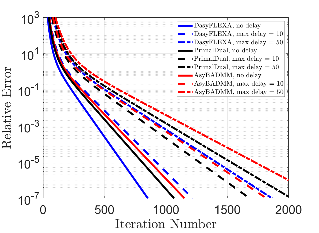
Figure 1: LASSO problem: Relative error vs. # of iterations.

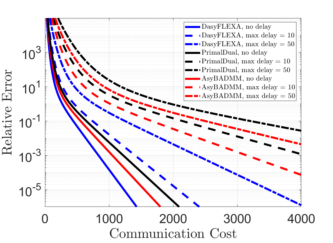
Figure 2: LASSO problem: Relative error vs. # of message exchanges.

DAsyFLEXA outperforms the PrimalDual scheme [36] and AsyBADMM [41]. Also, as anticipated, PrimalDual requires much more communications than DAsyFLEXA.

IV-B Distributed Matrix Completion

In this section we consider the Distributed Matrix Completion problem (1). We generate a $2200\times 2200$ matrix $\mathbf{Z}$ with samples drawn from $\mathcal{N}(0,1)$; and we set $\lambda=\xi=1$ and $r=4$. Each core of our cluster computer represents a different agent; the columns of $\mathbf{X}$ and $\mathbf{Y}$ are equally partitioned across the 22 cores, and those of $\mathbf{Y}$ uniformly among the other 11 cores; and all cores access a shared memory where the data are stored. We sampled uniformly at random 10% of the entries of $\mathbf{Z}$, and distributed these samples $z_{mn}$ to the agents owing the corresponding column $\mathbf{x}_{m}$ of $\mathbf{X}$ or $\mathbf{y}_{n}$ of $\mathbf{Y}$, choosing randomly between the two.

We applied the following instance of DAsyFLEXA to (1). Consider one of the agents that optimizes some columns of $\mathbf{X}$, say agent $i$. Since each $f_{i}$ is biconvex in $\mathbf{X}$ and $\mathbf{Y}$, the following surrogate function satisfies Assumption C:

$$\tilde{f}_{i}\left(\{\mathbf{x}_{m}\}_{m\in X_{i}};(\mathbf{X},\mathbf{Y})_{\mathcal{N}_{i}}^{k-\mathbf{d}^{k}(i,i)}\right)$$ (10)

$$=\!\dfrac{1}{2}\sum\limits_{(m,n)\in\Omega_{i}}\!\!\!\!\left(\mathbf{x}_{m}^{T}\mathbf{y}_{n}^{k-d_{j(n)}^{k}(i,i)}\!-\!z_{mn}\right)^{2}\!\!+\dfrac{\tau_{i}}{2}\!\!\!\!\sum\limits_{(m,n)\in\Omega_{i}}\!\!\!\!\!\|\mathbf{x}_{m}\!-\!\mathbf{x}_{m}^{k}\|_{2}^{2};$$

where $j(n)$ is the index $j\in\mathcal{N}_{i}$ of the agent that controls $\mathbf{y}_{n}$, and $\tau_{i}>0$ is updated following the same heuristic used in [49] (the surrogate function for the agents that update columns of $\mathbf{Y}$ is the same as (10), with the obvious change of variables). Note that (10) preserves the block-wise convexity present in the original function $f_{i}$, which contrasts with the common approach in the literature based on the linearization of $f_{i}$. Problem (5) with the surrogate (10) has a closed-form solution.

We compare our algorithm with the decentralized ADMM version of ARock, as presented in [37]. Even if this method has convergence guarantees for convex problems only, its performances on this experiment appeared to be good. For ARock we fixed $\eta^{k}=0.9$, for all $k$, and $\gamma=10$, which are the values that gave us the best performances in the experiments.

The rest of the setup is the same as that described for the LASSO problem. Figure 3 and Figure 4 plot $\|\widehat{\mathbf{x}}^{k}-\mathbf{x}^{k}\|_{\infty}$ (a valid measure of stationarity), with $\widehat{\mathbf{x}}_{i}$ defined as in (5), obtained by DAsyFLEXA and the PrimalDual algorithm [36] versus the CPU time (measured in seconds) and message exchanges per agent. On our tests, we observed that all the algorithms converged to the same stationary solution. The results confirm the behavior observed in the previous section for convex problems: DAsyFLEXA has better performances than PrimalDual, and the difference is mostly significant is terms of communication cost. DAsyFLEXA is also more efficient than ARock, which suffers from a similar drawback of PrimalDual for what concerns the number of message exchanges; this is due to the fact that ARock requires the use of dual variables, which cause a communication overhead.

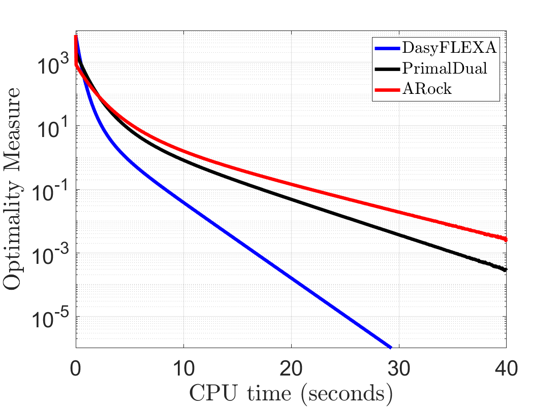
Figure 3: Matrix completion: stationarity distance vs. # CPU time (in seconds).

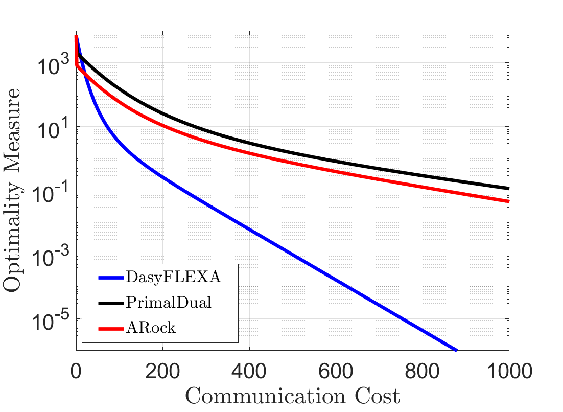
Figure 4: Matrix completion: stationarity distance vs. # of message exchanges.

V Appendix

In this Appendix we prove Theorems 2 and 3.

V-A Notation

Vectors $\mathbf{x}_{\mathcal{N}_{j}}^{k-\mathbf{d}^{k}(i,j)}$ have different length. It is convenient to replace them with equal-length vectors retaining of course the same information. This is done introducing the following (column) vectors $\mathbf{x}^{k}(i,j)\triangleq(\mathbf{x}^{k}_{l}(i,j))_{l=1}^{N}\in\mathcal{X}$, defined as:

$$[\mathbf{x}^{k}_{l}(i,j)]_{l\in\mathcal{N}_{j}}\triangleq\mathbf{x}_{\mathcal{N}_{j}}^{k-\mathbf{d}^{k}(i,j)},$$ (11a)

$$\mathbf{x}_{l}^{k}(i,j)=\mathbf{x}^{k}_{l},\quad l\notin\mathcal{N}_{j}.$$ (11b)

In words, the blocks of $\mathbf{x}^{k}(i,j)$ indexed by $\mathcal{N}_{j}$ coincide with $\mathbf{x}_{\mathcal{N}_{j}}^{k-\mathbf{d}^{k}(i,j)}$ whereas the other block-components, irrelevant to the proofs, are conveniently set to their most up-to-date values. We will use the shorthand $\mathbf{x}_{\mathcal{N}_{j}}^{k}(i,j)\triangleq[\mathbf{x}^{k}_{l}(i,j)]_{l\in\mathcal{N}_{j}}$.

Since at each iteration $k\geq 0$ only one block of $\mathbf{x}^{k}$ is updated, and because of Assumption D2, it is not difficult to check that the delayed vector $\mathbf{x}^{k}(i,j)$ can be written as

$$\mathbf{x}^{k}(i,j)=\mathbf{x}^{k}+\sum\limits_{l\in\mathcal{K}^{k}(i,j)}(\mathbf{x}^{l}-\mathbf{x}^{l+1}),\vspace{-0.1cm}$$ (12)

where $\mathcal{K}^{k}(i,j)$ is a subset of $\{k-D,\ldots,k-1\}$ whose elements depend on which block variables have been updated in the window $[\max\{0,k-D\},\max\{0,k-1\}]$. Recall that it is assumed $\mathbf{x}^{t}=\mathbf{x}^{0}$, for $t<0$.

Finally, notice that the notation $\widehat{\mathbf{x}}_{i}^{k}$ for the best-response map (5) is a shorthand for the formal expression $\widehat{\mathbf{x}}_{i}(\tilde{\mathbf{x}}^{k}(i))$, where $\tilde{\mathbf{x}}^{k}(i)\triangleq\left[\mathbf{x}_{\mathcal{N}_{j}}^{k-\mathbf{d}^{k}(i,j)}\right]_{j\in\mathcal{N}_{i}}$. Similarly, $\widehat{\bar{\mathbf{x}}}_{i}^{k}$ (resp. $\widehat{\bar{\mathbf{x}}}^{k}$) in (7) is a shorthand for $\widehat{\mathbf{x}}_{i}(\bar{\mathbf{x}}^{k}(i))$ (resp. $\widehat{\mathbf{x}}(\bar{\mathbf{x}}^{k})$), where $\bar{\mathbf{x}}^{k}(i)\triangleq\left[\mathbf{x}^{k}_{\mathcal{N}_{j}}\right]_{j\in\mathcal{N}_{i}}$ (resp. $\bar{\mathbf{x}}^{k}\triangleq\left[\bar{\mathbf{x}}^{k}(i)\right]_{i\in\mathcal{N}}$). We also define the following shorthands:

$$\Delta\widehat{\mathbf{x}}^{k}\triangleq\left[\Delta\widehat{\mathbf{x}}_{i}^{k}\right]_{i\in\mathcal{N}},\quad\Delta\widehat{\mathbf{x}}_{i}^{k}\triangleq\widehat{\mathbf{x}}_{i}^{k}-\mathbf{x}_{i}^{k}.$$ (13)

Table I summarizes the main notation used in the paper. On the constant $L$. The proofs rely on some Lipschitz properties of $\nabla_{\mathbf{x}_{j}}f_{i}$’s. To provide a unified proof under either A2(a) or A2(b), we introduce a constant $L>0$ whose value depends on whether A2(a) or A2(b) hold. Specifically:
$\bullet$ A2(a) holds: the gradients $\nabla_{\mathbf{x}_{j}}f_{i}$’s are not globally Lipschitz on the sets $\mathcal{X}_{\mathcal{N}_{i}}$’s; our approach to study convergence is to ensure that they are Lipschitz continuous on suitably defined sets containing the sequences generated by Algorithm 1. We define these sets as follows. Define first the set $\texttt{Cube}\triangleq\left\{\mathbf{w}\in\mathcal{X}:\|\mathbf{w}\|_{\infty}\leq U\right\}$, where $U$ is positive constant that ensures $\mathcal{L}^{0}\subseteq\texttt{Cube}$ (note that $U<+\infty$ because $\mathcal{L}^{0}$ is bounded). Then, we define a proper widening $\bar{\mathcal{L}}^{0}$ of $\mathcal{L}^{0}$: $\bar{\mathcal{L}}^{0}\triangleq\left(\mathcal{L}^{0}+\psi\mathcal{B}\right)\cap\mathcal{X}$, where $\mathcal{B}$ is the unitary ball centered in the origin, and $\psi>0$ is a finite positive constant defined as

$$\psi\triangleq\underset{i\in\mathcal{N}}{\max}\;\underset{\begin{subarray}{c}\tilde{\mathbf{w}}(i)\triangleq[\mathbf{w}_{\mathcal{N}_{j}}(j)]_{j\in\mathcal{N}_{i}}\\ \mathbf{w}(j)\in\texttt{Cube}\end{subarray}}{\max}\;\|\widehat{\mathbf{x}}_{i}\left(\tilde{\mathbf{w}}(i)\right)-\mathbf{w}_{i}(i)\|_{2}.$$ (14)

Note that $\bar{\mathcal{L}}^{0}$ is compact, because $\mathcal{L}^{0}$ is bounded and $\psi<+\infty$ [given that Cube is bounded and $\widehat{\mathbf{x}}(\cdot)$ is continuous, due to (5), A2, A3, and C3]. Consider now any vector $\mathbf{x}\in\bar{\mathcal{L}}^{0}$. A2(a) and compactness of $\bar{\mathcal{L}}^{0}$ imply that the gradients $\nabla_{\mathbf{x}_{j}}f_{i}$’s are globally Lipschitz over the sets containing the subvectors $\mathbf{x}_{\mathcal{N}_{i}}$’s, with $L$ being the maximum value of the Lipschitz constant of all the gradients over these sets.
$\bullet$ A2(b) holds: In this case, $L$ is simply the global Lipschitz constant $\nabla_{\mathbf{x}_{i}}f_{i}$ over the whole space.

Symbol	Definition
$V(\mathbf{x})$, cf. (P)	$F(\mathbf{x})+G(\mathbf{x})$
$F(\mathbf{x})$, cf. (P)	$\sum\limits_{i=1}^{N}f_{i}\left(\mathbf{x}_{\mathcal{N}_{i}}\right)$
$G(\mathbf{x})$, cf. (P)	$\sum\limits_{i=1}^{N}g_{i}\left(\mathbf{x}_{i}\right)$
$\mathbf{x}$, cf. (P)	Optimization variable
$\mathbf{x}_{i}$, cf. (P)	Block-variable of agent $i$
$\mathbf{x}_{\mathcal{N}_{i}}$, cf. (P)	Block-variables of agent $i$’s set of neighbors: $[\mathbf{x}_{j}]_{j\in\mathcal{N}_{i}}$
$\mathbf{x}_{\mathcal{N}_{j}}^{k-\mathbf{d}^{k}(i,j)}$	Agent $i$’s local copy of agent $j$’s vector $\mathbf{x}_{\mathcal{N}_{j}}^{k}$, possibly delayed
$\mathbf{x}^{k}(i,j)$, cf. (11)	Same as $\mathbf{x}_{\mathcal{N}_{j}}^{k-\mathbf{d}^{k}(i,j)}$, with the addition of slack elements to fix dimensionality
$\widehat{\mathbf{x}}_{i}^{k}/\widehat{\mathbf{x}}_{i}(\tilde{\mathbf{x}}^{k}(i))$, cf. (5)	Solution of subproblem (5)
$\tilde{\mathbf{x}}^{k}(i)$	Agent $i$’s local copies of his neighbors vectors $[\mathbf{x}_{\mathcal{N}_{j}}^{k}]_{j\in\mathcal{N}_{i}}$, possibly delayed: $\left[\mathbf{x}_{\mathcal{N}_{j}}^{k-\mathbf{d}^{k}(i,j)}\right]_{j\in\mathcal{N}_{i}}$
$\bar{\mathbf{x}}^{k}$	Collection of all the $\tilde{\mathbf{x}}^{k}(i)$’s: $\left[\bar{\mathbf{x}}^{k}(i)\right]_{i\in\mathcal{N}}$
$\widehat{\bar{\mathbf{x}}}_{i}^{k}/\widehat{\mathbf{x}}_{i}(\bar{\mathbf{x}}^{k}(i))$, cf. (7)	Solution of subproblem (5) wherein all the delays are set to 0
$\bar{\mathbf{x}}^{k}(i)$	Same structure of $\tilde{\mathbf{x}}^{k}(i)$ wherein all the delays are set to 0
$\bar{\mathbf{x}}^{k}$	Collection of all the $\bar{\mathbf{x}}^{k}(i)$’s: $\left[\bar{\mathbf{x}}^{k}(i)\right]_{i\in\mathcal{N}}$

TABLE I: Table of notation

Remark 4.

To make sense of the complicated definition of $L$ under A2(a), we anticipate how this constant will be used. Our proof leverages the decent lemma to majorize $V(\mathbf{x}^{k+1})$. To do so, each $\nabla_{{\mathbf{x}}_{j}}f_{i}$ needs to be globally Lipschitz on a convex set containing ${\mathbf{x}}^{k}$ and ${\mathbf{x}}^{k+1}$. This is what the convex set $\bar{\mathcal{L}}^{0}$ is meant for: ${\mathbf{x}}^{k}$ and ${\mathbf{x}}^{k+1}$ belong to $\bar{\mathcal{L}}^{0}$ and thus $\nabla_{{\mathbf{x}}_{j}}f_{i}$ is $L$-Lipschitz continuous.

V-B Preliminaries

We summarize next some properties of the map $\widehat{\mathbf{x}}_{i}^{k}$ in (5).

Proposition 5.

Given Problem (P) under Assumption A, let $\{\mathbf{x}^{k}\}$ be the sequence generated by DAsyFLEXA, under Assumptions B and C. Suppose also that $\mathbf{x}^{k}\in\bar{\mathcal{L}}^{0}$ for all $k$. There hold:

• [Optimality] For any $i\in\mathcal{N}$ and $k\geq 0$,

  $$\sum\limits_{j\in\mathcal{N}_{i}}\left\langle\nabla_{\mathbf{x}_{i}}f_{j}(\mathbf{x}^{k}_{\mathcal{N}_{j}}(i,j)),\Delta\widehat{\mathbf{x}}^{k}_{i}\right\rangle$$

  $$+g_{i}(\widehat{\mathbf{x}}_{i}^{k})-g_{i}(\mathbf{x}^{k}_{i})\leq-\tau\|\Delta\widehat{\mathbf{x}}_{i}^{k}\|_{2}^{2};$$ (15)

• [Lipschitz continuity] For any $i\in\mathcal{N}$ and $k,h\geq 0$,

  $$\|\widehat{\mathbf{x}}_{i}^{k}-\widehat{\mathbf{x}}_{i}^{h}\|_{2}\leq\frac{L_{m}}{\tau}\|\mathbf{x}^{k}(i,i)-\mathbf{x}^{h}(i,i)\|_{2}$$

  $$\qquad+\frac{L}{\tau}\sum\limits_{j\in\mathcal{N}_{i}\backslash\{i\}}\|\mathbf{x}^{k}(i,j)-\mathbf{x}^{k}(i,j)\|_{2},$$ (16)

  where $L_{m}\triangleq\underset{i\in\mathcal{N}}{\max}\,L_{i}$;

• [Fixed-points] $\widehat{\mathbf{x}}(\bar{\mathbf{x}}^{k})=\mathbf{x}^{k}$ if and only if $\mathbf{x}^{k}$ is a stationary solutions of Problem (P) (recall the definition of $\bar{\mathbf{x}}^{k}$ in Table I);

• [Error bound] For any $k\geq 0$,

  $$\|\mathbf{x}^{k}-\text{{prox}}_{G}\left(\mathbf{x}^{k}-\nabla F(\mathbf{x}^{k})\right)\|_{2}$$

  $$\leq(1+L+NL_{m})\|\widehat{\mathbf{x}}(\bar{\mathbf{x}}^{k})-\mathbf{x}^{k}\|_{2}.$$ (17)

Proof.

We prove only (d); the proof of (a)-(c) follows similar steps of that in [48, Proposition 8], and thus is omitted. Invoking the optimality of $\widehat{\mathbf{x}}(\bar{\mathbf{x}}^{k})$, we have

$$\Bigg{\langle}\nabla\tilde{f}_{i}\left(\widehat{\mathbf{x}}_{i}(\bar{\mathbf{x}}^{k}(i));\mathbf{x}^{k}_{\mathcal{N}_{i}}\right)+\sum\limits_{j\in\mathcal{N}_{i}\backslash\{i\}}\nabla_{\mathbf{x}_{i}}f_{j}\left(\mathbf{x}^{k}_{\mathcal{N}_{j}}\right),$$

$$\widehat{\mathbf{x}}_{i}(\bar{\mathbf{x}}^{k}(i))-\mathbf{z}_{i}\Bigg{\rangle}+g_{i}(\widehat{\mathbf{x}}_{i}(\bar{\mathbf{x}}^{k}(i)))-g_{i}(\mathbf{z}_{i})\leq 0,$$

for all $\mathbf{z}\in\mathcal{X}$ and $i\in\mathcal{N}$. Setting $\check{\mathbf{x}}^{k}\triangleq\texttt{prox}_{G}\left(\mathbf{x}^{k}-\nabla F(\mathbf{x}^{k})\right)$, and invoking the variational characterization of the proximal operator, we have

$$\left\langle\nabla_{\mathbf{x}}F(\mathbf{x}^{k})+\check{\mathbf{x}}^{k}-\mathbf{x}^{k},\check{\mathbf{x}}^{k}-\mathbf{w}\right\rangle+G(\check{\mathbf{x}}^{k})-G(\mathbf{w})\leq 0,$$

for all $\mathbf{w}\in\mathcal{X}$. Summing the two inequalities above, with $\mathbf{z}=\check{\mathbf{x}}^{k}$, $\mathbf{w}=\widehat{\mathbf{x}}(\bar{\mathbf{x}}^{k})$, and using C1 and C2, yields

$$\tau\|\widehat{\mathbf{x}}(\bar{\mathbf{x}}^{k})-\mathbf{x}^{k}\|_{2}^{2}+\|\check{\mathbf{x}}^{k}-\mathbf{x}^{k}\|_{2}^{2}$$

$$\leq\|\check{\mathbf{x}}^{k}-\mathbf{x}^{k}\|_{2}\|\widehat{\mathbf{x}}(\bar{\mathbf{x}}^{k}(i))-\mathbf{x}^{k}\|_{2}+\sum\limits_{i=1}^{N}\Big{\langle}\nabla\tilde{f}_{i}(\widehat{\mathbf{x}}_{i}(\bar{\mathbf{x}}^{k}(i));\mathbf{x}^{k}_{\mathcal{N}_{i}})$$

$$\quad-\nabla\tilde{f}_{i}(\mathbf{x}_{i}^{k};\mathbf{x}^{k}_{\mathcal{N}_{i}}),\check{\mathbf{x}}_{i}^{k}-\mathbf{x}_{i}^{k}\Big{\rangle}$$

$$\stackrel{{\scriptstyle A2,C2-C3}}{{\leq}}\|\mathbf{x}^{k}-\check{\mathbf{x}}^{k}\|_{2}\left((1+L+NL_{m})\|\widehat{\mathbf{x}}(\bar{\mathbf{x}}^{k})-\mathbf{x}^{k}\|_{2}\right).$$

∎

V-C Proof of Theorem 2

The proof is organized in the following steps:

Step 1–Lyapunov function & its descent: We define an appropriate Lyapunov function $\tilde{V}$ and prove that it is monotonically nonincreasing along the iterations. This also proves Theorem 2(c);

Step 2–Vanishing $\mathbf{x}$-stationarity: Building on the descent properties of the Lyapunov function, we prove $\lim_{k\rightarrow+\infty}\|\widehat{\mathbf{x}}(\bar{\mathbf{x}}^{k})-\mathbf{x}^{k}\|_{2}=0$ [Theorem 2(a)];

Step 3–Convergence rate: We prove the sublinear convergence rate of $\{M_{V}(\mathbf{x}^{k})\}$ as stated in Theorem 2(c).

The above steps are proved under Assumptions A, C, and D.

V-C1 Step 1–Lyapunov function & its descent

Introduce the following Lyapunov-like function:

$$\tilde{V}(\mathbf{x}^{k},\dots,\mathbf{x}^{k-D}) \triangleq V(\mathbf{x}^{k})+\frac{DL\rho^{2}}{2}\Bigg{(}\sum\limits_{l=k-D}^{k-1}\big{(}l-(k-1)$$

$$+D\big{)}\|\mathbf{x}^{l+1}-\mathbf{x}^{l}\|_{2}^{2}\Bigg{)},$$ (18)

where $L$ is defined in Sec.V-A. Note that

$$\tilde{V}^{\star}\triangleq\underset{[\mathbf{y}^{i}\in\mathcal{X}]_{i=1}^{D+1}}{\min}\,\tilde{V}(\mathbf{y}^{1},\ldots,\mathbf{y}^{D+1})=\underset{\mathbf{x}\in\mathcal{X}}{\min}\,V(\mathbf{x}).$$

The following lemma establishes the descent properties of $\tilde{V}$ and also proves Theorem 2(c).

Lemma 6.

Given $\tilde{V}$ defined in (18), the following hold:
(a) For any $k\geq 0$:

$$\tilde{V}(\mathbf{x}^{k+1}\ldots,\mathbf{x}^{k+1-D})$$ (19)

$$\leq\tilde{V}(\mathbf{x}^{k},\ldots,\mathbf{x}^{k-D})-\gamma\left(\tau-\gamma\frac{L\left(2+D^{2}\rho^{2}\right)}{2}\right)\|\Delta\widehat{\mathbf{x}}_{i^{k}}^{k}\|_{2}^{2}.$$

(b) If, in particular, A2(a) is satisfied: $\mathbf{x}^{k}\in\mathcal{L}^{0},\,\text{for all}\,k\geq 0.$

Proof.

We prove the two statements by induction. For $k=0$,

$$V(\mathbf{x}^{1}) =\sum\limits_{i=1}^{N}f_{i}(\mathbf{x}^{1}_{\mathcal{N}_{i}})+g_{i^{0}}(\mathbf{x}_{i^{0}}^{1})+\sum\limits_{i\neq i^{0}}g_{i}(\mathbf{x}_{i}^{1})$$

$$\stackrel{{\scriptstyle\text{\eqref{update}}}}{{=}}\sum\limits_{i=1}^{N}f_{i}(\mathbf{x}^{1}_{\mathcal{N}_{i}})+g_{i^{0}}(\mathbf{x}_{i^{0}}^{1})+\sum\limits_{i\neq i^{0}}g_{i}(\mathbf{x}_{i}^{0})$$

$$\stackrel{{\scriptstyle\text{(a)}}}{{\leq}}\sum\limits_{i=1}^{N}f_{i}(\mathbf{x}^{0}_{\mathcal{N}_{i}})+\gamma\sum\limits_{j\in\mathcal{N}_{i^{0}}}\bigg{\langle}\nabla_{\mathbf{x}_{i^{0}}}f_{j}(\mathbf{x}^{0}_{\mathcal{N}_{j}})$$

$$\quad+\nabla_{\mathbf{x}_{i^{0}}}f_{j}\left(\mathbf{x}^{0}_{\mathcal{N}_{j}}(i^{0},j)\right)-\nabla_{\mathbf{x}_{i^{0}}}f_{j}\left(\mathbf{x}^{0}_{\mathcal{N}_{j}}(i^{0},j)\right),\Delta\widehat{\mathbf{x}}_{i^{0}}^{0}\bigg{\rangle}$$

$$\quad+\frac{\gamma^{2}L}{2}\|\Delta\widehat{\mathbf{x}}_{i^{0}}^{0}\|_{2}^{2}+g_{i^{0}}(\mathbf{x}_{i^{0}}^{1})+\sum\limits_{i\neq i^{0}}g_{i}(\mathbf{x}_{i}^{0})$$

$$\stackrel{{\scriptstyle\text{A3}}}{{\leq}}\sum\limits_{i=1}^{N}f_{i}(\mathbf{x}^{0}_{\mathcal{N}_{i}})+\gamma\left\langle\sum\limits_{j\in\mathcal{N}_{i^{0}}}\nabla_{\mathbf{x}_{i^{0}}}f_{j}\left(\mathbf{x}^{0}_{\mathcal{N}_{j}}(i^{0},j)\right),\Delta\widehat{\mathbf{x}}_{i^{0}}^{0}\right\rangle$$

$$\quad+\gamma\Big{\langle}\sum\limits_{j\in\mathcal{N}_{i^{0}}}\Big{(}\nabla_{\mathbf{x}_{i^{0}}}f_{j}(\mathbf{x}^{0}_{\mathcal{N}_{j}})$$

$$\quad-\nabla_{\mathbf{x}_{i^{0}}}f_{j}\left(\mathbf{x}^{0}_{\mathcal{N}_{j}}(i^{0},j)\right)\Big{)},\Delta\widehat{\mathbf{x}}_{i^{0}}^{0}\Big{\rangle}+\frac{\gamma^{2}L}{2}\|\Delta\widehat{\mathbf{x}}_{i^{0}}^{0}\|_{2}^{2}$$

$$\quad+\sum\limits_{i=1}^{N}g_{i}(\mathbf{x}_{i}^{0})+\gamma g_{i^{0}}(\widehat{\mathbf{x}}_{i^{0}}^{0})-\gamma g_{i^{0}}(\mathbf{x}^{0}_{i^{0}})$$

$$\stackrel{{\scriptstyle\eqref{comments},A2}}{{\leq}}V(\mathbf{x}^{0})-\gamma\left(\tau-\frac{\gamma L}{2}\right)\|\Delta\widehat{\mathbf{x}}_{i^{0}}^{0}\|_{2}^{2}$$

$$\quad+\gamma L\|\Delta\widehat{\mathbf{x}}_{i^{0}}^{0}\|_{2}\sum\limits_{j\in\mathcal{N}_{i^{0}}}\|\mathbf{x}^{0}-\mathbf{x}^{0}(i^{0},j)\|_{2}$$

$$\stackrel{{\scriptstyle\text{(b)}}}{{\leq}}V(\mathbf{x}^{0})-\gamma\left(\tau-\gamma L\right)\|\Delta\widehat{\mathbf{x}}_{i^{0}}^{0}\|_{2}^{2}$$

$$\quad+\frac{L\rho}{2}\sum\limits_{j\in\mathcal{N}_{i^{0}}}\underbrace{\|\mathbf{x}^{0}-\mathbf{x}^{0}(i^{0},j)\|_{2}^{2}}_{\texttt{term I}},$$ (20)

where (a) follows from the descent lemma and the definition of $L$; and in (b) we used Young’s inequality. Note that in (a) we used the fact that $\mathbf{x}^{0}$ and $\mathbf{x}^{1}$ belong to $\bar{\mathcal{L}}^{0}$ (cf. Remark 4).

We now bound term I in (20). It is convenient to study the more general term $\|\mathbf{x}^{k}-\mathbf{x}^{k}(i^{k},j)\|_{2}^{2}$, $j\in\mathcal{N}_{i^{k}}$. There holds:

$$\|\mathbf{x}^{k}-\mathbf{x}^{k}(i^{k},j)\|_{2}^{2}\stackrel{{\scriptstyle\eqref{x_tilde}}}{{\leq}}\,\left(\sum\limits_{l=k-D}^{k-1}\|\mathbf{x}^{l+1}-\mathbf{x}^{l}\|_{2}\right)^{2}$$

$$\leq D\sum\limits_{l=k-D}^{k-1}\|\mathbf{x}^{l+1}-\mathbf{x}^{l}\|_{2}^{2}$$

$$=D\Bigg{(}\sum\limits_{l=k-D}^{k-1}\left(l-(k-1)+D\right)\|\mathbf{x}^{l+1}-\mathbf{x}^{l}\|_{2}^{2}$$

$$\quad-\sum\limits_{l=k+1-D}^{k}(l-k+D)\|\mathbf{x}^{l+1}-\mathbf{x}^{l}\|_{2}^{2}\Bigg{)}+D^{2}\|\mathbf{x}^{k+1}-\mathbf{x}^{k}\|^{2}_{2}.$$ (21)

Combining (20) and (21) one can check that statements (a) and (b) of the lemma hold at $k=0$, that is, $\tilde{V}\left(\mathbf{x}^{1},\ldots,\mathbf{x}^{0}\right)\leq\tilde{V}\left(\mathbf{x}^{0},\ldots,\mathbf{x}^{0}\right)$, and $V(\mathbf{x}^{1})\leq\tilde{V}\left(\mathbf{x}^{1},\ldots,\mathbf{x}^{0}\right)\leq\tilde{V}\left(\mathbf{x}^{0},\ldots,\mathbf{x}^{0}\right)=V(\mathbf{x}^{0})$, respectively.
Assume now that the two statements hold at iteration $k$. It is easy to check that the analogous of (20) also holds at iteration $k+1$ with the term $\sum\limits_{j\in\mathcal{N}_{i^{k}}}\|\mathbf{x}^{k}-\mathbf{x}^{k}(i^{k},j)\|_{2}$ in the analogous of term I at iteration $k$, majorized using (21). Combining (20) at $k+1$ with (21) one can check that statement (a) of the lemma holds at $k+1$. We also get: $V(\mathbf{x}^{k+1})\leq\tilde{V}\left(\mathbf{x}^{k+1},\ldots,\mathbf{x}^{k+1-D}\right)\stackrel{{\scriptstyle\eqref{prelyap_multi_02}}}{{\leq}}\tilde{V}\left(\mathbf{x}^{k},\ldots,\mathbf{x}^{k-D}\right)\leq\tilde{V}\left(\mathbf{x}^{0},\ldots,\mathbf{x}^{0}\right)=V(\mathbf{x}^{0})$, which proves statement (b) of the lemma at $k+1$. This completes the proof. ∎

V-C2 Step 2 – Vanishing $\mathbf{x}$-stationarity

It follows from A4 and Lemma 6 that, if $\gamma<\frac{2\tau}{L\left(2+\rho^{2}D^{2}\right)}$, $\{\tilde{V}(\mathbf{x}^{k-D},\ldots,\mathbf{x}^{k})\}$ and thus $\{V(\mathbf{x}^{k})\}$ converge. Therefore,

$$\lim\limits_{k\rightarrow+\infty}\|\Delta\widehat{\mathbf{x}}_{i^{k}}^{k}\|_{2}=0.$$ (22)

The next lemma extends the vanishing properties of a single block $\Delta\widehat{\mathbf{x}}^{k}_{i^{k}}$ to the entire vector $\Delta\widehat{\mathbf{x}}^{k}$.

Lemma 7.

For any $i\in\mathcal{N},k\geq 0$, and $h,t\in[k,k+B-1]$, there hold:

$$\|\widehat{\mathbf{x}}_{i}(\tilde{\mathbf{x}}^{t}(i))-\widehat{\mathbf{x}}_{i}(\tilde{\mathbf{x}}^{h}(i))\|_{2}^{2}\leq C_{2}\sum\limits_{l=k-D}^{k+B-2}\|\Delta\widehat{\mathbf{x}}^{l}_{i^{l}}\|_{2}^{2},\vspace{-0.2cm}$$ (23)

$$\|\Delta\widehat{\mathbf{x}}^{h}\|_{2}^{2}\leq 2\Big{(}NC_{2}+1\Big{)}\sum\limits_{l=k-D}^{k+B-1}\|\Delta\widehat{\mathbf{x}}^{l}_{i^{l}}\|_{2}^{2}.\vspace{-0.3cm}$$ (24)

with

$$C_{2}\triangleq\frac{3\gamma^{2}(B+2D-N+1)\rho\left(L_{m}^{2}+(\rho-1)L^{2}\right)}{\tau^{2}}.$$

Proof.

See Section V-E. ∎

Using (24) and (22) yields

$$\lim\limits_{k\rightarrow+\infty}\|\Delta\widehat{\mathbf{x}}^{k}\|_{2}=0.$$ (25)

Furthermore, invoking (22), (23), and (25) together with $\|\widehat{\mathbf{x}}(\bar{\mathbf{x}}^{k})-\mathbf{x}^{k}\|_{2}\leq\|\Delta\widehat{\mathbf{x}}^{k}\|_{2}+\|\widehat{\mathbf{x}}(\bar{\mathbf{x}}^{k})-\widehat{\mathbf{x}}^{k}\|_{2}$, leads to

$$\lim\limits_{k\rightarrow+\infty}\|\widehat{\mathbf{x}}(\bar{\mathbf{x}}^{k})-\mathbf{x}^{k}\|_{2}=0,$$ (26)

which, together with Proposition 5(c), proves Theorem 2(a).

V-C3 Step 3 – Convergence rate

We use the Lyapunov function $\tilde{V}$ to study the vanishing rate of $\{M_{V}(\mathbf{x}^{k})\}$. Due to (26) and the definition of $M_{V}$, we know that $M_{V}$ is converging to 0. Therefore $T_{\epsilon}$ is finite. Using $M_{V}(\mathbf{x}^{k})>\epsilon$, for all $k\in\{0,\ldots,T_{\epsilon}-1\}$, we have

$$T_{\epsilon}\epsilon \leq\sum\limits_{k=0}^{T_{\epsilon}-1}M_{V}(\mathbf{x}^{k})\leq 2\sum\limits_{k=0}^{T_{\epsilon}-1}\left(\|\Delta\widehat{\mathbf{x}}^{k}\|_{2}^{2}+\|\widehat{\mathbf{x}}(\bar{\mathbf{x}}^{k})-\widehat{\mathbf{x}}^{k}\|_{2}^{2}\right)$$

$$\stackrel{{\scriptstyle\eqref{lipsch},\eqref{fourth_bis_a}}}{{\leq}}2\sum\limits_{k=0}^{T_{\epsilon}-1}\Bigg{(}2\left(NC_{2}+1\right)\sum\limits_{l=k-D}^{k+B-1}\|\Delta\widehat{\mathbf{x}}_{i^{l}}^{l}\|_{2}^{2}$$

$$\quad+\sum\limits_{i=1}^{N}\Bigg{(}\frac{L_{m}^{2}\rho}{\tau^{2}}\|\mathbf{x}^{k}(i,i)-\mathbf{x}^{k}\|_{2}^{2}$$

$$\quad+\frac{L^{2}\rho}{\tau^{2}}\sum\limits_{j\in\mathcal{N}_{i}\backslash\{i\}}\|\mathbf{x}^{k}(i,j)-\mathbf{x}^{k}\|_{2}^{2}\Bigg{)}\Bigg{)}$$

$$\stackrel{{\scriptstyle\eqref{x_tilde}}}{{\leq}}2\left(2\left(NC_{2}+1\right)+\frac{DC_{2}}{3(B+2D-N+1)}\right)$$

$$\quad\cdot\sum\limits_{k=0}^{T_{\epsilon}-1}\sum\limits_{l=k-D}^{k+B-1}\|\Delta\widehat{\mathbf{x}}^{l}_{i^{l}}\|_{2}^{2}$$

$$\stackrel{{\scriptstyle(a)}}{{\leq}}C_{3}\sum\limits_{k=0}^{T_{\epsilon}-1}\sum\limits_{l=k-D}^{k+B-1}\Bigg{(}\tilde{V}\left(\mathbf{x}^{l},\ldots,\mathbf{x}^{l-D}\right)$$

$$\qquad-\tilde{V}\left(\mathbf{x}^{l+1},\ldots,\mathbf{x}^{l+1-D}\right)\Bigg{)}$$

$$=C_{3}\sum\limits_{k=0}^{T_{\epsilon}-1}\Bigg{(}\tilde{V}\left(\mathbf{x}^{k-D},\ldots,\mathbf{x}^{k-2D}\right)$$

$$\qquad-\tilde{V}\left(\mathbf{x}^{k+B},\ldots,\mathbf{x}^{k+B-D}\right)\Bigg{)}$$

$$\leq C_{3}(B+D-1)\left(V(\mathbf{x}^{0})-\underset{\mathbf{x}\in\mathcal{X}}{\min}\,V(\mathbf{x})\right),$$ (27)

where in (a) we used (19) and defined $C_{3}$ as

$$C_{3}\triangleq\frac{4\left(2\left(NC_{2}+1\right)+\frac{DC_{2}}{3(B+2D-N+1)}\right)}{\gamma\left(2\tau-\gamma L\left(2+D^{2}\rho^{2}\right)\right)}.$$

Statement (b) of the theorem follows readily by defining

$$C_{1}\triangleq C_{3}(B+D-1).$$ (28)

V-D Proof of Theorem 3

We study now convergence of Algorithm 1 under the additional Assumption B.

First of all, note that one can always find $\eta,\epsilon,\kappa>0$ such that B1 holds. In fact, i) by Lemma 6, there exist some $\eta$ and sufficiently small $\gamma/\tau$ such that $V(\mathbf{x}^{k})\leq\eta$, for all $k\geq 0$; and ii) since $\|\mathbf{x}^{k}-\texttt{prox}_{G}\left(\nabla F(\mathbf{x}^{k})-\mathbf{x}^{k}\right)\|_{2}$ is asymptotically vanishing [Proposition 5(d) and (26)], one can always find some $\epsilon>0$ such that $\|\mathbf{x}^{k}-\texttt{prox}_{G}\left(\nabla F(\mathbf{x}^{k})-\mathbf{x}^{k}\right)\|_{2}\leq\epsilon$, for all $k\geq 0$.

The proof proceeds along the following steps. Step 1: We first show that the liminf of $\left\{V(\mathbf{x}^{k})\right\}$ is a stationary point $V^{\star}$, see (33). Step 2 shows that $\left\{V(\mathbf{x}^{k})\right\}$ approaches $V^{\star}$ linearly, up to an error of the order $\mathcal{O}\left(\sum\limits_{l=k-D}^{k+B-1}\|\Delta\widehat{\mathbf{x}}^{l}_{i_{l}}\|_{2}^{2}\right)$, see (37). Finally, in Step 3 we show that the term $\sum\limits_{l=k-D}^{k+B-1}\|\Delta\widehat{\mathbf{x}}^{l}_{i_{l}}\|_{2}^{2}$ is overall vanishing at a geometric rate, implying the convergence of $\left\{V(\mathbf{x}^{k})\right\}$ to $V^{\star}$ at a geometric rate.

V-D1 Step 1

Pick any vector $\mathbf{x}^{\star}(\mathbf{x}^{k})\in P_{\mathcal{X}^{\star}}(\mathbf{x}^{k})$, where $P_{\mathcal{X}^{\star}}(\mathbf{x})\triangleq{\arg\min}_{\mathbf{x}^{\star}\in\mathcal{X}^{\star}}\|\mathbf{x}-\mathbf{x}^{\star}\|_{2}$, $\mathbf{x}\in\mathbb{R}^{n}$. Note that:

$$d(\mathbf{x}^{k},\mathcal{X}^{\star})=\|\mathbf{x}^{\star}(\mathbf{x}^{k})-\mathbf{x}^{k}\|_{2}\stackrel{{\scriptstyle B1}}{{\leq}}\kappa\|\mathbf{x}^{k}-\texttt{prox}_{G}\left(\nabla_{\mathbf{x}}F(\mathbf{x}^{k})-\mathbf{x}^{k}\right)\|_{2}.$$ (29)

Using (29), (26), and (17), yields

$$\underset{k\rightarrow+\infty}{\lim}\,\|\mathbf{x}^{\star}(\mathbf{x}^{k})-\mathbf{x}^{\star}(\mathbf{x}^{k+1})\|=0.$$ (30)

This, together with B2, imply that there exists an index $\bar{k}\geq 0$ and a scalar $V^{\star}$ such that

$$V(\mathbf{x}^{\star}(\mathbf{x}^{k}))=V^{\star},\quad\forall\,k\geq\bar{k}.$$ (31)

By the Mean Value Theorem, there exists a vector $\boldsymbol{\xi}^{k}=\beta^{k}\mathbf{x}^{\star}(\mathbf{x}^{k})+(1-\beta^{k})\mathbf{x}^{k}$, for some $\beta^{k}\in(0;1)$, such that, for any $k\geq\bar{k}$,

$$V^{\star}-V(\mathbf{x}^{k})=\left\langle\nabla_{\mathbf{x}}F(\boldsymbol{\xi}^{k}),\mathbf{x}^{\star}(\mathbf{x}^{k})-\mathbf{x}^{k}\right\rangle+G(\mathbf{x}^{\star}(\mathbf{x}^{k}))$$

$$-G(\mathbf{x}^{k})\leq\left\langle\nabla_{\mathbf{x}}F(\boldsymbol{\xi}^{k})-\nabla_{\mathbf{x}}F(\mathbf{x}^{\star}(\mathbf{x}^{k})),\mathbf{x}^{\star}(\mathbf{x}^{k})-\mathbf{x}^{k}\right\rangle$$

$$\stackrel{{\scriptstyle(a)}}{{\leq}}\frac{N(\rho^{2}L^{2}+1)}{2}\|\mathbf{x}^{\star}(\mathbf{x}^{k})-\mathbf{x}^{k}\|_{2}^{2}$$

$$\stackrel{{\scriptstyle\eqref{lemma3},\eqref{errbdnew}}}{{\leq}}\frac{N\kappa(\rho^{2}L^{2}+1)(1+L+NL_{m})}{2}\|\widehat{\mathbf{x}}(\bar{\mathbf{x}})^{k}-\mathbf{x}^{k}\|_{2},$$ (32)

where (a) follows from A2 and $\|\boldsymbol{\xi}^{k}-\mathbf{x}^{\star}(\mathbf{x}^{k})\|_{2}^{2}=\|\beta^{k}{\mathbf{x}}^{\star}(\mathbf{x}^{k})+(1-\beta^{k}){\mathbf{x}}^{k}-\mathbf{x}^{\star}(\mathbf{x}^{k})\|_{2}^{2}\leq\|\mathbf{x}^{\star}(\mathbf{x}^{k})-{\mathbf{x}}^{k}\|_{2}^{2}.$

By invoking (32), together with (26), we obtain

$$\underset{k\rightarrow+\infty}{\lim\inf}\,V(\mathbf{x}^{k})\geq V^{\star}.$$ (33)

V-D2 Step 2

We next show that $V(\mathbf{x}^{k})$ approaches $V^{\star}$ at a linear rate.

To this end, consider (20) with $0$ and $1$ replaced by $k$ and $k+1$ respectively; we have the following:

$$V(\mathbf{x}^{k+1})\leq V(\mathbf{x}^{k})-\gamma\left(\tau-\gamma L\right)\|\Delta\widehat{\mathbf{x}}_{i^{k}}\|_{2}^{2}$$

$$+\frac{L\rho}{2}\sum\limits_{j\in\mathcal{N}_{i^{k}}}\|\mathbf{x}^{k}-\mathbf{x}^{k}(i^{k},j)\|_{2}^{2}\stackrel{{\scriptstyle\eqref{x_tilde}}}{{\leq}}V(\mathbf{x}^{k})$$

$$-\gamma\left(\tau-\gamma L\right)\|\Delta\widehat{\mathbf{x}}_{i^{k}}\|_{2}^{2}+\frac{\gamma^{2}DL\rho^{2}}{2}\sum\limits_{l=k-D}^{k-1}\|\Delta\widehat{\mathbf{x}}_{i^{l}}^{l}\|_{2}^{2}.$$ (34)

Is easy to see that, for any $k\geq\bar{k}$, (34) implies:

$$V(\mathbf{x}^{k+B})-V^{\star}\leq V(\mathbf{x}^{k})-V^{\star}$$

$$-\gamma\left(\tau-\frac{\gamma L(2+BD\rho^{2})}{2}\right)\sum\limits_{l=k}^{k+B-1}\|\Delta\widehat{\mathbf{x}}_{i^{l}}^{l}\|_{2}^{2}$$

$$+\frac{B\gamma^{2}DL\rho^{2}}{2}\sum\limits_{l=k-D}^{k-1}\|\Delta\widehat{\mathbf{x}}_{i^{l}}^{l}\|_{2}^{2}.$$ (35)

To prove the desired result we will combine next (35) with the following lemma.

Lemma 8.

For any $k\geq 0$, there holds:

$$V(\mathbf{x}^{k+B})-V(\mathbf{x}^{\star}(\mathbf{x}^{k}))\leq(1-\gamma)\left(V(\mathbf{x}^{k})-V(\mathbf{x}^{\star}(\mathbf{x}^{k}))\right)$$

$$+\gamma\left(N\alpha_{1}+(B-N)\alpha_{2}\right)\sum\limits_{l=k-D}^{k+B-1}\|\Delta\widehat{\mathbf{x}}_{i^{l}}^{l}\|_{2}^{2},$$ (36)

where $\alpha_{1}$ and $\alpha_{2}$ are two positive constants defined in Appendix V-E [see (61) and (63), respectively].

Proof.

See Section V-E. ∎

Multiplying the two sides of (35) and (36) by $(N\alpha_{1}+(B-N)\alpha_{2})$ and $\tau-\gamma L(2+BD\rho^{2})/2$ respectively, and adding the two inequalities together, yields

$$V(\mathbf{x}^{k+B})-V^{\star}\leq\theta\left(V(\mathbf{x}^{k})-V^{\star}\right)+\zeta\sum\limits_{l=k-D}^{k-1}\|\Delta\widehat{\mathbf{x}}_{i^{l}}^{l}\|_{2}^{2},$$ (37)

for all $k\geq\bar{k}$, where

$$\theta\triangleq\frac{(1-\gamma)(2\tau-\gamma L(BD\mathcal{N}^{2}_{m}+2))+2N\alpha_{1}+2(B-N)\alpha_{2}}{2\tau-\gamma L(BD\mathcal{N}^{2}_{m}+2)+2N\alpha_{1}+2(B-N)\alpha_{2}},$$

and

$$\zeta\triangleq\frac{(N\alpha_{1}+(B-N)\alpha_{2})(2\tau+\gamma L(BD\rho^{2}(\gamma-1)+2))}{2\tau-\gamma L(BD\mathcal{N}^{2}_{m}+2)+2N\alpha_{1}+2(B-N)\alpha_{2}}.$$

V-D3 Step 3

We can now apply Lemma 4.5 in [6] by noticing that (35), (33), and (37) correspond, respectively, to (4.21), (4.22), and to the first inequality after (4.23) in [6]. Theorem 3 readily follows, setting

$$\lambda\triangleq 1-\frac{\gamma^{2}}{2}\frac{2\tau-\gamma L(BD\rho^{2}+2)}{2N\alpha_{1}+2(B-N)\alpha_{2}}$$

$$\cdot\frac{}{+\gamma(2-\gamma)(2\tau-\gamma L(BD\rho^{2}+2))}.$$ (38)

V-E Miscellanea results

This section contains the proofs of Lemma 7 and Lemma 8.

Proof of Lemma 7: (i) Assume without loss of generality that $t\leq h$. We have

$$\|\widehat{\mathbf{x}}_{i}(\tilde{\mathbf{x}}^{t}(i))-\widehat{\mathbf{x}}_{i}(\tilde{\mathbf{x}}^{h}(i))\|_{2}^{2}\stackrel{{\scriptstyle\eqref{lipsch}}}{{\leq}}\frac{\rho L_{m}^{2}}{\tau^{2}}\|\mathbf{x}^{t}(i,i)-\mathbf{x}^{h}(i,i)\|_{2}^{2}$$

$$+\frac{\rho L^{2}}{\tau^{2}}\sum\limits_{j\in\mathcal{N}_{i}\backslash\{i\}}\|\mathbf{x}^{t}(i,j)-\mathbf{x}^{h}(i,j)\|_{2}^{2}$$

$$\stackrel{{\scriptstyle\eqref{x_tilde},\eqref{update}}}{{\leq}}\left(\frac{3\rho\left(L_{m}^{2}+(\rho-1)L^{2}\right)}{\tau^{2}}\right)\Bigg{(}\gamma^{2}(B-N+1)$$

$$\sum\limits_{l=t}^{h-1}\|\Delta\widehat{\mathbf{x}}_{i^{l}}^{l}\|_{2}^{2}+D\gamma^{2}\left(\sum\limits_{l=t-D}^{t-1}\|\Delta\widehat{\mathbf{x}}_{i^{l}}^{l}\|^{2}_{2}+\sum\limits_{l=h-D}^{h-1}\|\Delta\widehat{\mathbf{x}}_{i^{l}}^{l}\|_{2}^{2}\right)\Bigg{)}.$$

(ii) Define $r_{i}^{h,k}\triangleq\underset{t\in[k;k+B-1]:i^{t}=i}{\arg\min}\,|t-h|$. We have:

$$\|\Delta\widehat{\mathbf{x}}^{h}\|_{2}^{2} \leq 2\sum\limits_{i=1}^{N}\left(\|\widehat{\mathbf{x}}_{i}^{h}-\widehat{\mathbf{x}}_{i}^{r_{i}^{h,k}}\|_{2}^{2}+\|\Delta\widehat{\mathbf{x}}_{i}^{r^{h,k}_{i}}\|_{2}^{2}\right)$$ (39)

$$\stackrel{{\scriptstyle\eqref{lip}}}{{\leq}}2\sum\limits_{i=1}^{N}\Bigg{(}C_{2}\sum\limits_{l=k-D}^{k+B-2}\|\Delta\widehat{\mathbf{x}}_{i^{l}}^{l}\|_{2}^{2}+\|\Delta\widehat{\mathbf{x}}_{i}^{r_{i}^{h,k}}\|_{2}^{2}\Bigg{)}.$$

Proof of Lemma 8: Define $T_{i}^{k}+1$ as the number of times agent $i$ performs its update within $[k,k+B-1]$; let $l^{k}_{i,0},\ldots,l^{k}_{i,T_{i}^{k}}$,be the iteration indexes of such updates. By the Mean Value Theorem, there exists a vector $\boldsymbol{\xi}^{k}=\beta^{k}{{\mathbf{x}}}^{\star}({\mathbf{x}}^{k})+(1-\beta^{k})\mathbf{x}^{k}$, for some $\beta^{k}\in(0,1)$, such that

$$V(\mathbf{x}^{k+B})-V(\mathbf{x}^{\star}(\mathbf{x}^{k}))=\left\langle\nabla_{\mathbf{x}}F(\boldsymbol{\xi}^{k}),\mathbf{x}^{k+B}-\mathbf{x}^{\star}(\mathbf{x}^{k})\right\rangle$$

$$+G(\mathbf{x}^{k+B})-G(\mathbf{x}^{\star}(\mathbf{x}^{k}))$$

$$=\sum\limits_{i=1}^{N}\Bigg{(}\underbrace{\left\langle\nabla_{\mathbf{x}_{i}}F(\boldsymbol{\xi}^{k}),\mathbf{x}_{i}^{l^{k}_{i,1}}-\mathbf{x}_{i}^{\star}(\mathbf{x}^{k})\right\rangle}_{\texttt{term II}}$$

$$\quad+\sum\limits_{t=1}^{T_{i}^{k}-1}\underbrace{\left\langle\nabla_{\mathbf{x}_{i}}F(\boldsymbol{\xi}^{k}),\mathbf{x}^{l^{k}_{i,t+1}}_{i}-\mathbf{x}_{i}^{l^{k}_{i,t}}\right\rangle}_{\texttt{term III}}$$

$$\quad+\underbrace{\left\langle\nabla_{\mathbf{x}_{i}}F(\boldsymbol{\xi}^{k}),\mathbf{x}^{k+B}_{i}-\mathbf{x}_{i}^{l^{k}_{i,T_{i}^{k}}}\right\rangle}_{\texttt{term IV}}\Bigg{)}$$

$$\quad+G(\mathbf{x}^{k+B})-G(\mathbf{x}^{\star}(\mathbf{x}^{k})).$$ (40)

To prove (36), it is then sufficient show that term II, term III, and term IV in (40) converge at a geometric rate up to an error of the order $\mathcal{O}\left(\sum\limits_{l=k-D}^{k+B-1}\|\Delta\widehat{\mathbf{x}}^{l}_{i_{l}}\|_{2}^{2}\right)$. To do this, we first show that term II, term III, and term IV converges at a geometric rate up to the error terms $a_{i,4}^{k}$, $b_{i,t,4}^{k}$, and $c_{i,4}^{k}$, respectively [see (41), (44), and (47)]. Then, we prove that each of these errors is of the order $\mathcal{O}\left(\sum\limits_{l=k-D}^{k+B-1}\|\Delta\widehat{\mathbf{x}}^{l}_{i_{l}}\|_{2}^{2}\right)$, as desired [see (60), and (62)].

Term II can be upper bounded as

$$\left\langle\nabla_{\mathbf{x}_{i}}F(\boldsymbol{\xi}^{k}),\mathbf{x}^{l^{k}_{i,1}}_{i}-\mathbf{x}_{i}^{\star}(\mathbf{x}^{k})\right\rangle$$

$$\stackrel{{\scriptstyle A2}}{{\leq}}\left\langle\nabla_{\mathbf{x}_{i}}F\left(\widehat{\mathbf{x}}^{l^{k}_{i,0}}\right),\mathbf{x}^{l^{k}_{i,1}}_{i}-\mathbf{x}_{i}^{\star}(\mathbf{x}^{k})\right\rangle$$

$$\quad+\underbrace{\rho L\left\|\widehat{\mathbf{x}}^{l^{k}_{i,0}}-\boldsymbol{\xi}^{k}\right\|_{2}\left\|\mathbf{x}^{l^{k}_{i,1}}_{i}-\mathbf{x}_{i}^{\star}(\mathbf{x}^{k})\right\|_{2}}_{\triangleq a_{i,1}^{k}}$$

$$\stackrel{{\scriptstyle A2,C2,C3}}{{\leq}}\Bigg{\langle}\nabla\tilde{f}_{i}\left(\widehat{\mathbf{x}}_{i}^{l^{k}_{i,0}};\mathbf{x}^{l^{k}_{i,0}}_{\mathcal{N}_{i}}(i,i)\right)$$

$$\quad+\sum\limits_{j\in\mathcal{N}_{i}\backslash\{i\}}\nabla_{\mathbf{x}_{i}}f_{j}\left(\mathbf{x}^{l_{i,0}^{k}}_{\mathcal{N}_{j}}(i,j)\right),\mathbf{x}_{i}^{l^{k}_{i,1}}-\mathbf{x}_{i}^{\star}(\mathbf{x}^{k})\Bigg{\rangle}$$

$$\quad+\left\|\mathbf{x}^{l^{k}_{i,1}}_{i}-\mathbf{x}_{i}^{\star}(\mathbf{x}^{k})\right\|_{2}\Bigg{(}L_{i}\left\|\widehat{\mathbf{x}}^{l_{i,0}^{k}}_{\mathcal{N}_{i}}-\mathbf{x}^{l^{k}_{i,0}}_{\mathcal{N}_{i}}(i,i)\right\|_{2}$$

$$\quad+L\sum\limits_{j\in\mathcal{N}_{i}\backslash\{i\}}\left\|\widehat{\mathbf{x}}_{\mathcal{N}_{j}}^{l_{i,0}^{k}}-\mathbf{x}^{l_{i,0}^{k}}_{\mathcal{N}_{j}}(i,j)\right\|_{2}\Bigg{)}+a_{i,1}^{k}$$

$$\stackrel{{\scriptstyle(a)}}{{\leq}}(\gamma-1)\Bigg{\langle}\nabla\tilde{f}_{i}\left(\widehat{\mathbf{x}}_{i}^{l^{k}_{i,0}};\mathbf{x}^{l^{k}_{i,0}}_{\mathcal{N}_{i}}(i,i)\right)$$

$$\quad+\sum\limits_{j\in\mathcal{N}_{i}\backslash\{i\}}\nabla_{\mathbf{x}_{i}}f_{j}\left(\mathbf{x}^{l_{i,0}^{k}}_{\mathcal{N}_{j}}(i,j)\right),\Delta\widehat{\mathbf{x}}_{i}^{l^{k}_{i,0}}\Bigg{\rangle}+g_{i}\left(\mathbf{x}_{i}^{\star}(\mathbf{x}^{k})\right)$$

$$\quad-g_{i}\left(\widehat{\mathbf{x}}_{i}^{l^{k}_{i,0}}\right)+a_{i,2}^{k}\stackrel{{\scriptstyle C2}}{{\leq}}g_{i}(\mathbf{x}_{i}^{\star}(\mathbf{x}^{k}))-g_{i}\left(\widehat{\mathbf{x}}_{i}^{l^{k}_{i,0}}\right)$$

$$+(\gamma-1)\left\langle\sum\limits_{j\in\mathcal{N}_{i}}\nabla_{\mathbf{x}_{i}}f_{j}\left(\mathbf{x}^{l^{k}_{i,0}}_{\mathcal{N}_{j}}(i,j)\right),\Delta\widehat{\mathbf{x}}^{l^{k}_{i,0}}_{i}\right\rangle$$

$$+(1-\gamma)\Bigg{\|}\nabla\tilde{f}_{i}\left(\widehat{\mathbf{x}}_{i}^{l^{k}_{i,0}};\mathbf{x}^{l^{k}_{i,0}}_{\mathcal{N}_{i}}(i,i)\right)-\nabla\tilde{f}_{i}\left(\mathbf{x}_{i}^{l^{k}_{i,0}};\mathbf{x}^{l^{k}_{i,0}}_{\mathcal{N}_{i}}(i,i)\right)\Bigg{\|}_{2}$$

$$\cdot\left\|\Delta\widehat{\mathbf{x}}^{l^{k}_{i,0}}_{i}\right\|_{2}+a_{i,2}^{k}\stackrel{{\scriptstyle(b)}}{{\leq}}g_{i}\left(\mathbf{x}_{i}^{\star}(\mathbf{x}^{k})\right)-g_{i}\left(\widehat{\mathbf{x}}_{i}^{l^{k}_{i,0}}\right)$$

$$+\frac{1-\gamma}{\gamma}\left(V\left(\mathbf{x}^{l^{k}_{i,0}}\right)-V\left(\mathbf{x}^{l^{k}_{i,0}+1}\right)\right)$$

$$+(1-\gamma)\left\|\sum\limits_{j\in\mathcal{N}_{i}}\left(\nabla_{\mathbf{x}_{i}}f_{j}\left(\mathbf{x}^{l^{k}_{i,0}}_{\mathcal{N}_{j}}\right)-\nabla_{\mathbf{x}_{i}}f_{j}\left(\mathbf{x}^{l^{k}_{i,0}}_{\mathcal{N}_{j}}(i,j)\right)\right)\right\|_{2}$$

$$\cdot\left\|\Delta\widehat{\mathbf{x}}_{i}^{l^{k}_{i,0}}\right\|_{2}+\frac{L\gamma(1-\gamma)}{2}\left\|\Delta\widehat{\mathbf{x}}_{i}^{l^{k}_{i,0}}\right\|_{2}^{2}+a_{i,3}^{k}$$

$$+(1-\gamma)\left(g_{i}\left(\widehat{\mathbf{x}}_{i}^{l^{k}_{i,0}}\right)-g_{i}\left(\mathbf{x}_{i}^{l^{k}_{i,0}}\right)\right)$$

$$\stackrel{{\scriptstyle(c)}}{{=}}\frac{1-\gamma}{\gamma}\left(V\left(\mathbf{x}^{l^{k}_{i,0}}\right)-V\left(\mathbf{x}^{l^{k}_{i,0}+1}\right)\right)+g_{i}\left(\mathbf{x}_{i}^{\star}(\mathbf{x}^{k})\right)$$

$$\quad+(\gamma-1)g_{i}\left(\mathbf{x}_{i}^{l^{k}_{i,0}}\right)-\gamma g_{i}\left(\widehat{\mathbf{x}}_{i}^{l^{k}_{i,0}}\right)+a_{i,4}^{k};$$ (41)

where the quantities $a_{i,2}^{k}$ in (a), and $a_{i,3}^{k}$ in (b) are defined in (42) and (43) at the bottom of the next page, respectively; furthermore in (b) we used the descent lemma, and in (c) we defined

$$a_{i,4}^{k}\triangleq\,a_{i,3}^{k}+\frac{L\gamma(1-\gamma)}{2}\left\|\Delta\widehat{\mathbf{x}}_{i}^{l^{k}_{i,0}}\right\|_{2}^{2}+(1-\gamma)$$

$$\cdot\underbrace{\left\|\sum\limits_{j\in\mathcal{N}_{i}}\left(\nabla_{\mathbf{x}_{i}}f_{j}\left(\mathbf{x}^{l^{k}_{i,0}}_{\mathcal{N}_{j}}\right)-\nabla_{\mathbf{x}_{i}}f_{j}\left(\mathbf{x}^{l^{k}_{i,0}}_{\mathcal{N}_{j}}(i,j)\right)\right)\right\|_{2}\left\|\Delta\widehat{\mathbf{x}}_{i}^{l^{k}_{i,0}}\right\|_{2}}_{\texttt{term VII}}.$$

 

$$a_{i,2}^{k}\triangleq a_{i,1}^{k}+\underbrace{\left\|\mathbf{x}^{l^{k}_{i,1}}_{i}-\mathbf{x}_{i}^{\star}(\mathbf{x}^{k})\right\|_{2}\left(L_{i}\left\|\widehat{\mathbf{x}}^{l_{i,0}^{k}}_{\mathcal{N}_{i}}-\mathbf{x}^{l^{k}_{i,0}}_{\mathcal{N}_{i}}(i,i)\right\|_{2}+L\sum\limits_{j\in\mathcal{N}_{i}\backslash\{i\}}\left\|\widehat{\mathbf{x}}_{\mathcal{N}_{j}}^{l_{i,0}^{k}}-\mathbf{x}^{l_{i,0}^{k}}_{\mathcal{N}_{j}}(i,j)\right\|_{2}\right)}_{\texttt{term V}}$$ (42)

$$a_{i,3}^{k}\triangleq a_{i,2}^{k}+(1-\gamma)\underbrace{\bigg{\|}\nabla\tilde{f}_{i}\left(\widehat{\mathbf{x}}_{i}^{l^{k}_{i,0}};\mathbf{x}^{l^{k}_{i,0}}_{\mathcal{N}_{i}}(i,i)\right)-\nabla\tilde{f}_{i}\left(\mathbf{x}_{i}^{l^{k}_{i,0}};\mathbf{x}^{l^{k}_{i,0}}_{\mathcal{N}_{i}}(i,i)\right)\bigg{\|}_{2}\left\|\Delta\widehat{\mathbf{x}}^{l^{k}_{i,0}}_{i}\right\|_{2}}_{\texttt{term VI}}$$ (43)

Term III can be upper bounded as: for any $i$ and $t\in[1,T^{k}_{i}-1]$,

$$\left\langle\nabla_{\mathbf{x}_{i}}F(\boldsymbol{\xi}^{k}),\mathbf{x}^{l^{k}_{i,t+1}}_{i}-\mathbf{x}_{i}^{l^{k}_{i,t}}\right\rangle$$

$$\stackrel{{\scriptstyle A2}}{{\leq}}\left\langle\nabla_{\mathbf{x}_{i}}F\left(\widehat{\mathbf{x}}^{l^{k}_{i,t}}\right),\mathbf{x}^{l^{k}_{i,t+1}}_{i}-\mathbf{x}_{i}^{l^{k}_{i,t}}\right\rangle$$

$$\quad+\underbrace{\rho L\left\|\widehat{\mathbf{x}}^{l^{k}_{i,t}}-\boldsymbol{\xi}^{k}\right\|_{2}\left\|\mathbf{x}^{l^{k}_{i,t}}_{i}-\mathbf{x}_{i}^{l^{k}_{i,t+1}}\right\|_{2}}_{\triangleq b_{i,t,1}^{k}}$$

$$\stackrel{{\scriptstyle A2,C2,C3}}{{\leq}}\Bigg{\langle}\nabla\tilde{f}_{i}\left(\widehat{\mathbf{x}}_{i}^{l^{k}_{i,t}};\mathbf{x}^{l^{k}_{i,t}}_{\mathcal{N}_{i}}(i,i)\right)$$

$$\quad+\sum\limits_{j\in\mathcal{N}_{i}\backslash\{i\}}\nabla_{\mathbf{x}_{i}}f_{j}\left(\mathbf{x}_{\mathcal{N}_{j}}^{l_{i,t}^{k}}(i,j)\right),\mathbf{x}_{i}^{l^{k}_{i,t+1}}-\mathbf{x}_{i}^{l^{k}_{i,t}}\Bigg{\rangle}$$

$$\quad+\left\|\mathbf{x}^{l^{k}_{i,t}}_{i}-\mathbf{x}_{i}^{l^{k}_{i,t+1}}\right\|_{2}\Bigg{(}L_{i}\left\|\widehat{\mathbf{x}}^{l_{i,t}^{k}}_{\mathcal{N}_{i}}-\mathbf{x}^{l^{k}_{i,t}}_{\mathcal{N}_{i}}(i,i)\right\|_{2}$$

$$\quad+L\sum\limits_{j\in\mathcal{N}_{i}\backslash\{i\}}\left\|\widehat{\mathbf{x}}^{l_{i,t}^{k}}_{\mathcal{N}_{j}}-\mathbf{x}^{l_{i,t}^{k}}_{\mathcal{N}_{j}}(i,j)\right\|_{2}\Bigg{)}+b_{i,t,1}^{k}$$

$$\stackrel{{\scriptstyle(a)}}{{\leq}}(\gamma-1)\Bigg{\langle}\nabla\tilde{f}_{i}\left(\widehat{\mathbf{x}}_{i}^{l^{k}_{i,t}};\mathbf{x}^{l^{k}_{i,t}}_{\mathcal{N}_{i}}(i,i)\right)$$

$$\quad+\sum\limits_{j\in\mathcal{N}_{i}\backslash\{i\}}\nabla_{\mathbf{x}_{i}}f_{j}\left(\mathbf{x}_{\mathcal{N}_{j}}^{l_{i,t}^{k}}(i,j)\right),\Delta\widehat{\mathbf{x}}_{i}^{l^{k}_{i,t}}\Bigg{\rangle}+g_{i}\left(\mathbf{x}_{i}^{l^{k}_{i,t}}\right)$$

$$\quad-g_{i}\left(\widehat{\mathbf{x}}_{i}^{l^{k}_{i,t}}\right)+b_{i,t,2}^{k}\stackrel{{\scriptstyle C2}}{{\leq}}g_{i}\left(\mathbf{x}_{i}^{l^{k}_{i,t}}\right)-g_{i}\left(\widehat{\mathbf{x}}_{i}^{l^{k}_{i,t}}\right)$$

$$+(\gamma-1)\left\langle\sum\limits_{j\in\mathcal{N}_{i}}\nabla_{\mathbf{x}_{i}}f_{j}\left(\mathbf{x}_{\mathcal{N}_{j}}^{l^{k}_{i,t}}(i,j)\right),\Delta\widehat{\mathbf{x}}^{l^{k}_{i,t}}_{i}\right\rangle$$

$$+(1-\gamma)\left\|\nabla\tilde{f}_{i}\left(\widehat{\mathbf{x}}_{i}^{l^{k}_{i,t}};\mathbf{x}^{l^{k}_{i,t}}_{\mathcal{N}_{i}}(i,i)\right)-\nabla\tilde{f}_{i}\left(\mathbf{x}_{i}^{l^{k}_{i,t}};\mathbf{x}^{l^{k}_{i,t}}_{\mathcal{N}_{i}}(i,i)\right)\right\|_{2}$$

$$\cdot\left\|\Delta\widehat{\mathbf{x}}^{l^{k}_{i,t}}_{i}\right\|_{2}+b_{i,t,2}^{k}\stackrel{{\scriptstyle(b)}}{{\leq}}g_{i}\left(\mathbf{x}_{i}^{l^{k}_{i,t}}\right)-g_{i}\left(\widehat{\mathbf{x}}_{i}^{l^{k}_{i,t}}\right)$$

$$+\frac{1-\gamma}{\gamma}\left(V\left(\mathbf{x}^{l^{k}_{i,t}}\right)-V\left(\mathbf{x}^{l^{k}_{i,t}+1}\right)\right)$$

$$+(1-\gamma)\left\|\sum\limits_{j\in\mathcal{N}_{i}}\left(\nabla_{\mathbf{x}_{i}}f_{j}\left(\mathbf{x}^{l^{k}_{i,t}}_{\mathcal{N}_{j}}\right)-\nabla_{\mathbf{x}_{i}}f_{j}\left(\mathbf{x}^{l^{k}_{i,t}}_{\mathcal{N}_{j}}(i,j)\right)\right)\right\|_{2}$$

$$\left\|\Delta\widehat{\mathbf{x}}_{i}^{l^{k}_{i,t}}\right\|_{2}+\frac{L\gamma(1-\gamma)}{2}\left\|\Delta\widehat{\mathbf{x}}_{i}^{l^{k}_{i,t}}\right\|_{2}^{2}+b_{i,t,3}^{k}$$

$$+(1-\gamma)\left(g_{i}\left(\widehat{\mathbf{x}}_{i}^{l^{k}_{i,t}}\right)-g_{i}\left(\mathbf{x}_{i}^{l^{k}_{i,t}}\right)\right)$$

$$=\frac{1-\gamma}{\gamma}\left(V\left(\mathbf{x}^{l^{k}_{i,t}}\right)-V\left(\mathbf{x}^{l^{k}_{i,t}+1}\right)\right)$$

$$\quad+\gamma\left(g_{i}\left(\mathbf{x}_{i}^{l^{k}_{i,t}}\right)-g_{i}\left(\widehat{\mathbf{x}}_{i}^{l^{k}_{i,t}}\right)\right)+b_{i,t,4}^{k};$$ (44)

where the quantities $b_{i,t,2}^{k}$ in (a), and $b_{i,t,3}^{k}$ in (b) are defined in (45) and (46) at the bottom of the next page, respectively; furthermore in (b) we used the descent lemma, and in (c) we defined

$$b_{i,t,4}^{k}\triangleq\,b_{i,t,3}^{k}+\frac{L\gamma(1-\gamma)}{2}\left\|\Delta\widehat{\mathbf{x}}_{i}^{l^{k}_{i,t}}\right\|_{2}^{2}+(1-\gamma)$$

$$\cdot\underbrace{\left\|\sum\limits_{j\in\mathcal{N}_{i}}\left(\nabla_{\mathbf{x}_{i}}f_{j}\left(\mathbf{x}^{l^{k}_{i,t}}_{\mathcal{N}_{j}}\right)-\nabla_{\mathbf{x}_{i}}f_{j}\left(\mathbf{x}^{l^{k}_{i,t}}_{\mathcal{N}_{j}}(i,j)\right)\right)\right\|_{2}\left\|\Delta\widehat{\mathbf{x}}_{i}^{l^{k}_{i,t}}\right\|_{2}}_{\texttt{term VII}}.$$

 

$$b_{i,t,2}^{k}\triangleq b_{i,t,1}^{k}+\underbrace{\left\|\mathbf{x}^{l^{k}_{i,t}}_{i}-\mathbf{x}_{i}^{l^{k}_{i,t+1}}\right\|_{2}\left(L_{i}\left\|\widehat{\mathbf{x}}^{l_{i,t}^{k}}_{\mathcal{N}_{i}}-\mathbf{x}^{l^{k}_{i,t}}_{\mathcal{N}_{i}}(i,i)\right\|_{2}+L\sum\limits_{j\in\mathcal{N}_{i}\backslash\{i\}}\left\|\widehat{\mathbf{x}}^{l_{i,t}^{k}}_{\mathcal{N}_{j}}-\mathbf{x}^{l_{i,t}^{k}}_{\mathcal{N}_{j}}(i,j)\right\|_{2}\right)}_{\texttt{term VIII}}$$ (45)

$$b_{i,t,3}^{k}\triangleq b_{i,t,2}^{k}+(1-\gamma)\underbrace{\left\|\nabla\tilde{f}_{i}\left(\widehat{\mathbf{x}}_{i}^{l^{k}_{i,t}};\mathbf{x}^{l^{k}_{i,t}}_{\mathcal{N}_{i}}(i,i)\right)-\nabla\tilde{f}_{i}\left(\mathbf{x}_{i}^{l^{k}_{i,t}};\mathbf{x}^{l^{k}_{i,t}}_{\mathcal{N}_{i}}(i,i)\right)\right\|_{2}\left\|\Delta\widehat{\mathbf{x}}^{l^{k}_{i,t}}_{i}\right\|_{2}}_{\texttt{term VI}}$$ (46)

Following similar steps, we can bound term IV, as

$$\left\langle\nabla_{\mathbf{x}_{i}}F(\boldsymbol{\xi}^{k}),\mathbf{x}^{k+B}_{i}-\mathbf{x}_{i}^{l^{k}_{i,T_{i}^{k}}}\right\rangle$$

$$\stackrel{{\scriptstyle A2}}{{\leq}}\left\langle\nabla_{\mathbf{x}_{i}}F\left(\widehat{\mathbf{x}}^{l^{k}_{i,T^{k}_{i}}}\right),\mathbf{x}^{k+B}_{i}-\mathbf{x}_{i}^{l^{k}_{i,T^{k}_{i}}}\right\rangle$$

$$\quad+\underbrace{\rho L\left\|\widehat{\mathbf{x}}^{l^{k}_{i,T^{k}_{i}}}-\boldsymbol{\xi}^{k}\right\|_{2}\left\|\mathbf{x}^{l^{k}_{i,T^{k}_{i}}}_{i}-\mathbf{x}_{i}^{k+B}\right\|_{2}}_{c_{i,1}^{k}}$$

$$\stackrel{{\scriptstyle A2,C2,C3}}{{\leq}}\Bigg{\langle}\nabla\tilde{f}_{i}\left(\widehat{\mathbf{x}}_{i}^{l^{k}_{i,T^{k}_{i}}};\mathbf{x}^{l^{k}_{i,T^{k}_{i}}}_{\mathcal{N}_{i}}(i,i)\right)$$

$$\quad+\sum\limits_{j\in\mathcal{N}_{i}\backslash\{i\}}\nabla_{\mathbf{x}_{i}}f_{j}\left(\mathbf{x}_{\mathcal{N}_{j}}^{l_{i,T^{k}_{i}}^{k}}(i,j)\right),\mathbf{x}_{i}^{k+B}-\mathbf{x}_{i}^{l^{k}_{i,T^{k}_{i}}}\Bigg{\rangle}$$

$$\quad+\left\|\mathbf{x}^{l^{k}_{i,T^{k}_{i}}}_{i}-\mathbf{x}_{i}^{k+B}\right\|_{2}\Bigg{(}L_{i}\left\|\widehat{\mathbf{x}}^{l_{i,T^{k}_{i}}^{k}}_{\mathcal{N}_{i}}-\mathbf{x}^{l^{k}_{i,T^{k}_{i}}}_{\mathcal{N}_{i}}(i,i)\right\|_{2}$$

$$\quad+L\sum\limits_{j\in\mathcal{N}_{i}\backslash\{i\}}\left\|\widehat{\mathbf{x}}^{l_{i,T^{k}_{i}}^{k}}_{\mathcal{N}_{j}}-\mathbf{x}^{l_{i,T^{k}_{i}}^{k}}_{\mathcal{N}_{j}}(i,j)\right\|_{2}\Bigg{)}+c_{i,1}^{k}$$

$$\stackrel{{\scriptstyle(a)}}{{\leq}}(\gamma-1)\Bigg{\langle}\nabla\tilde{f}_{i}\left(\widehat{\mathbf{x}}_{i}^{l^{k}_{i,T^{k}_{i}}};\mathbf{x}^{l^{k}_{i,T^{k}_{i}}}_{\mathcal{N}_{i}}(i,i)\right)$$

$$\quad+\sum\limits_{j\in\mathcal{N}_{i}\backslash\{i\}}\nabla_{\mathbf{x}_{i}}f_{j}\left(\mathbf{x}_{\mathcal{N}_{j}}^{l_{i,T^{k}_{i}}^{k}}(i,j)\right),\Delta\widehat{\mathbf{x}}_{i}^{l^{k}_{i,T^{k}_{i}}}\Bigg{\rangle}+g_{i}\left(\mathbf{x}_{i}^{l^{k}_{i,T^{k}_{i}}}\right)$$

$$-g_{i}\left(\widehat{\mathbf{x}}_{i}^{l^{k}_{i,T^{k}_{i}}}\right)+c_{i,2}^{k}\stackrel{{\scriptstyle C2}}{{\leq}}g_{i}\left(\mathbf{x}_{i}^{l^{k}_{i,T^{k}_{i}}}\right)-g_{i}\left(\widehat{\mathbf{x}}_{i}^{l^{k}_{i,T^{k}_{i}}}\right)$$

$$+(\gamma-1)\left\langle\sum\limits_{j\in\mathcal{N}_{i}}\nabla_{\mathbf{x}_{i}}f_{j}\left(\mathbf{x}_{\mathcal{N}_{j}}^{l^{k}_{i,T^{k}_{i}}}(i,j)\right),\Delta\widehat{\mathbf{x}}^{l^{k}_{i,T^{k}_{i}}}_{i}\right\rangle$$

$$+(1-\gamma)\Bigg{\|}\nabla\tilde{f}_{i}\left(\widehat{\mathbf{x}}_{i}^{l^{k}_{i,T^{k}_{i}}};\mathbf{x}^{l^{k}_{i,T^{k}_{i}}}_{\mathcal{N}_{i}}(i,i)\right)-$$

$$\nabla\tilde{f}_{i}\left(\mathbf{x}_{i}^{l^{k}_{i,T^{k}_{i}}};\mathbf{x}^{l^{k}_{i,T^{k}_{i}}}_{\mathcal{N}_{i}}(i,i)\right)\Bigg{\|}_{2}\left\|\Delta\widehat{\mathbf{x}}^{l^{k}_{i,T^{k}_{i}}}_{i}\right\|_{2}+c_{i,2}^{k}\stackrel{{\scriptstyle(b)}}{{\leq}}g_{i}\left(\mathbf{x}_{i}^{l^{k}_{i,T^{k}_{i}}}\right)$$

$$-g_{i}\left(\widehat{\mathbf{x}}_{i}^{l^{k}_{i,T^{k}_{i}}}\right)+\frac{1-\gamma}{\gamma}\left(V\left(\mathbf{x}^{l^{k}_{i,T^{k}_{i}}}\right)-V\left(\mathbf{x}^{l^{k}_{i,T^{k}_{i}}+1}\right)\right)$$

$$+(1-\gamma)\left\|\sum\limits_{j\in\mathcal{N}_{i}}\left(\nabla_{\mathbf{x}_{i}}f_{j}\left(\mathbf{x}^{l^{k}_{i,T^{k}_{i}}}_{\mathcal{N}_{j}}\right)-\nabla_{\mathbf{x}_{i}}f_{j}\left(\mathbf{x}^{l^{k}_{i,T^{k}_{i}}}_{\mathcal{N}_{j}}(i,j)\right)\right)\right\|_{2}$$

$$\left\|\Delta\widehat{\mathbf{x}}_{i}^{l^{k}_{i,T^{k}_{i}}}\right\|_{2}+\frac{L\gamma(1-\gamma)}{2}\left\|\Delta\widehat{\mathbf{x}}_{i}^{l^{k}_{i,T^{k}_{i}}}\right\|_{2}^{2}+c_{i,3}^{k}$$

$$+(1-\gamma)\left(g_{i}\left(\widehat{\mathbf{x}}_{i}^{l^{k}_{i,T^{k}_{i}}}\right)-g_{i}\left(\mathbf{x}_{i}^{l^{k}_{i,T^{k}_{i}}}\right)\right)$$

$$=\frac{1-\gamma}{\gamma}\left(V\left(\mathbf{x}^{l^{k}_{i,T^{k}_{i}}}\right)-V\left(\mathbf{x}^{l^{k}_{i,T^{k}_{i}}+1}\right)\right)$$

$$\quad+\gamma\left(g_{i}\left(\mathbf{x}_{i}^{l^{k}_{i,T^{k}_{i}}}\right)-g_{i}\left(\widehat{\mathbf{x}}_{i}^{l^{k}_{i,T^{k}_{i}}}\right)\right)+c_{i,4}^{k};$$ (47)

where the quantities $c_{i,2}^{k}$ in (a), and $c_{i,3}^{k}$ in (b) are defined in (48) and (49) at the bottom of the next page, respectively; furthermore in (b) we used the descent lemma, and in (c) we defined

$$c_{i,4}^{k}\triangleq\,c_{i,3}^{k}+\frac{L\gamma(1-\gamma)}{2}\left\|\Delta\widehat{\mathbf{x}}_{i}^{l^{k}_{i,T^{k}_{i}}}\right\|_{2}^{2}+(1-\gamma)$$

$$\cdot\underbrace{\left\|\sum\limits_{j\in\mathcal{N}_{i}}\left(\nabla_{\mathbf{x}_{i}}f_{j}\left(\mathbf{x}^{l^{k}_{i,T^{k}_{i}}}_{\mathcal{N}_{j}}\right)-\nabla_{\mathbf{x}_{i}}f_{j}\left(\mathbf{x}^{l^{k}_{i,T^{k}_{i}}}_{\mathcal{N}_{j}}(i,j)\right)\right)\right\|_{2}\left\|\Delta\widehat{\mathbf{x}}_{i}^{l^{k}_{i,T^{k}_{i}}}\right\|_{2}}_{\texttt{term VII}}.$$

$$c_{i,2}^{k}\triangleq c_{i,1}^{k}+\underbrace{\left\|\mathbf{x}^{l^{k}_{i,T^{k}_{i}}}_{i}-\mathbf{x}_{i}^{k+B}\right\|_{2}\left(L_{i}\left\|\widehat{\mathbf{x}}^{l_{i,T^{k}_{i}}^{k}}_{\mathcal{N}_{i}}-\mathbf{x}^{l^{k}_{i,T^{k}_{i}}}_{\mathcal{N}_{i}}(i,i)\right\|_{2}+L\sum\limits_{j\in\mathcal{N}_{i}\backslash\{i\}}\left\|\widehat{\mathbf{x}}^{l_{i,T^{k}_{i}}^{k}}_{\mathcal{N}_{j}}-\mathbf{x}^{l_{i,T^{k}_{i}}^{k}}_{\mathcal{N}_{j}}(i,j)\right\|_{2}\right)}_{\texttt{term IX}}$$ (48)

$$c_{i,3}^{k}\triangleq c_{i,2}^{k}+(1-\gamma)\underbrace{\left\|\nabla\tilde{f}_{i}\left(\widehat{\mathbf{x}}_{i}^{l^{k}_{i,T^{k}_{i}}};\mathbf{x}^{l^{k}_{i,T^{k}_{i}}}_{\mathcal{N}_{i}}(i,i)\right)-\nabla\tilde{f}_{i}\left(\mathbf{x}_{i}^{l^{k}_{i,T^{k}_{i}}};\mathbf{x}^{l^{k}_{i,T^{k}_{i}}}_{\mathcal{N}_{i}}(i,i)\right)\right\|_{2}\left\|\Delta\widehat{\mathbf{x}}^{l^{k}_{i,T^{k}_{i}}}_{i}\right\|_{2}}_{\texttt{term VI}}$$ (49)

We now show that the error terms $a_{i,4}^{k}$, $b_{i,t,4}^{k}$, and $c_{i,4}^{k}$, are of the order $\mathcal{O}\left(\sum\limits_{l=k-D}^{k+B-1}\|\Delta\widehat{\mathbf{x}}^{l}_{i_{l}}\|_{2}^{2}\right)$. To do so, in the following we properly upper bound each term inside $a_{i,4}^{k}$, $b_{i,t,4}^{k}$, and $c_{i,4}^{k}$.

We begin noticing that, by the definition of $\boldsymbol{\xi}^{k}$, it follows

$$\|\widehat{\mathbf{x}}^{h}-\boldsymbol{\xi}^{k}\|_{2}$$

$$=\|(1-\beta^{k})\mathbf{x}^{k}+\beta^{k}\mathbf{x}^{\star}(\mathbf{x}^{k})-\widehat{\mathbf{x}}^{h}\|_{2}$$

$$\leq\|\mathbf{x}^{k}-\mathbf{x}^{\star}(\mathbf{x}^{k})\|_{2}+\|\widehat{\mathbf{x}}^{h}-\mathbf{x}^{k}\|_{2}$$

$$\leq\|\mathbf{x}^{k}-\mathbf{x}^{\star}(\mathbf{x}^{k})\|_{2}+\|\Delta\widehat{\mathbf{x}}^{h}\|+\|\mathbf{x}^{h}-\mathbf{x}^{k}\|,$$ (50)

for all $h\in[k;k+B-1]$.

1) Bounding $a_{i,1}^{k}$: there holds

$$a_{i,1}^{k}\stackrel{{\scriptstyle(a)}}{{\leq}}\frac{3\rho L}{2}\Bigg{(}2\|\mathbf{x}^{k}-\mathbf{x}^{\star}(\mathbf{x}^{k})\|_{2}^{2}+(1+\gamma^{2})\|\Delta\widehat{\mathbf{x}}^{l_{i,0}^{k}}\|_{2}^{2}$$

$$+2\|\mathbf{x}^{l^{k}_{i,0}}-\mathbf{x}^{k}\|_{2}^{2}\Bigg{)}\stackrel{{\scriptstyle(b)}}{{\leq}}3\rho L\Bigg{(}\kappa^{2}(1+L+NL_{m})^{2}\Big{(}\|\Delta\widehat{\mathbf{x}}^{k}\|_{2}^{2}$$

$$+C_{2}\sum\limits_{l=k-D}^{k+B-2}\|\Delta\widehat{\mathbf{x}}^{l}_{i^{l}}\|_{2}^{2}\Big{)}+(NC_{2}+1)(1+\gamma^{2})\sum\limits_{l=k-D}^{k+B-1}\|\Delta\widehat{\mathbf{x}}^{l}_{i^{l}}\|_{2}^{2}$$

$$+\gamma^{2}(B-N+1)\sum\limits_{l=k-D}^{k+B-2}\|\Delta\widehat{\mathbf{x}}^{l}_{i^{l}}\|_{2}^{2}\Bigg{)}\stackrel{{\scriptstyle(c)}}{{\leq}}\rho L\beta_{1}\sum\limits_{l=k-D}^{k+B-1}\|\Delta\widehat{\mathbf{x}}^{l}_{i^{l}}\|_{2}^{2},$$ (51)

where in (a) we used (50) and the Young’s inequality; (b) follows from (23), (24), and the fact that, for any $k\geq 0$,

$$\|\mathbf{x}^{k}-\mathbf{x}^{\star}(\mathbf{x}^{k})\|_{2}$$

$$\stackrel{{\scriptstyle B1}}{{\leq}}\kappa\|\mathbf{x}^{k}-\texttt{prox}_{G}\left(\nabla_{\mathbf{x}}F(\mathbf{x}^{k})-\mathbf{x}^{k}\right)\|_{2}$$

$$\stackrel{{\scriptstyle\eqref{lemma3}}}{{\leq}}\kappa(1+L+NL_{m})\|\widehat{\mathbf{x}}(\bar{\mathbf{x}}^{k})-\mathbf{x}^{k}\|_{2}$$

$$\leq\kappa(1+L+NL_{m})\left(\|\widehat{\mathbf{x}}(\bar{\mathbf{x}}^{k})-\widehat{\mathbf{x}}^{k}\|_{2}+\|\Delta\widehat{\mathbf{x}}^{k}\|_{2}\right);$$ (52)

and in (c) we used (24) and defined

$$\beta_{1}\triangleq C_{2}\Bigg{(}\kappa^{2}(1+L+NL_{m})^{2}(2N+1)+N(1+\gamma^{2})\Bigg{)}$$

$$+\kappa^{2}(1+L+NL_{m})^{2}+1+\gamma^{2}(B-N+2).$$

2) Bounding $b_{i,t,1}^{k}$ and $c_{i,1}^{k}$: for $t\in[1;T^{k}_{i}-1]$,

$$b_{i,t,1}^{k}\stackrel{{\scriptstyle(a)}}{{\leq}}\frac{\rho L}{2}\Big{(}3\|\mathbf{x}^{k}-\mathbf{x}^{\star}(\mathbf{x}^{k})\|_{2}^{2}+(3+\gamma^{2})\|\Delta\widehat{\mathbf{x}}^{l^{k}_{i,t}}\|_{2}^{2}$$

$$+3\|\mathbf{x}^{l^{k}_{i,t}}-\mathbf{x}^{k}\|_{2}^{2}\Big{)}\stackrel{{\scriptstyle(b)}}{{\leq}}\frac{\rho L}{2}\Bigg{(}6\kappa^{2}(1+L+NL_{m})^{2}\Bigg{(}\|\Delta\widehat{\mathbf{x}}^{k}\|_{2}^{2}$$

$$+C_{2}\sum\limits_{l=k-D}^{k+B-2}\|\Delta\widehat{\mathbf{x}}_{i^{l}}^{l}\|_{2}^{2}\Bigg{)}+2(NC_{2}+1)(3+\gamma^{2})\sum\limits_{l=k-D}^{k+B-1}\|\Delta\widehat{\mathbf{x}}_{i^{l}}^{l}\|_{2}^{2}$$

$$+3\gamma^{2}(B-N+1)\sum\limits_{l=k-D}^{k+B-2}\|\Delta\widehat{\mathbf{x}}_{i^{l}}^{l}\|_{2}^{2}\Bigg{)}\stackrel{{\scriptstyle(c)}}{{\leq}}\rho L\beta_{2}\sum\limits_{l=k-D}^{k+B-1}\|\Delta\widehat{\mathbf{x}}_{i^{l}}^{l}\|_{2}^{2},$$ (53)

where in (a) we used (50) and the Young’s inequality; (b) follows from (23), (24), (52); and in (c) we used (24) and defined

$$\beta_{2}\triangleq C_{2}\Bigg{(}3\kappa^{2}(1+L+NL_{m})^{2}(2N+1)+N(3+\gamma^{2})\Bigg{)}$$

$$+6\kappa^{2}(1+L+NL_{m})^{2}+3+\frac{\gamma^{2}}{2}(3B-3N+5).$$

Following the same steps as in (53), it is not difficult to prove:

$$c_{i,1}^{k}\leq\rho L\beta_{2}\sum\limits_{l=k-D}^{k+B-1}\|\Delta\widehat{\mathbf{x}}^{l}_{i^{l}}\|^{2}_{2}.$$ (54)

3) Bounding term V : there holds,

$$\texttt{term V}\stackrel{{\scriptstyle(a)}}{{\leq}}2\|\mathbf{x}^{k}-\mathbf{x}^{\star}(\mathbf{x}^{k})\|_{2}^{2}+2\gamma^{2}\left\|\Delta\widehat{\mathbf{x}}_{i}^{l^{k}_{i,0}}\right\|_{2}^{2}$$

$$+(L_{i}^{2}+L^{2}(\rho-1))\Bigg{(}\|\Delta\widehat{\mathbf{x}}^{l^{k}_{i,0}}\|_{2}^{2}+D\gamma^{2}\sum\limits_{l=l^{k}_{i,0}-D}^{l^{k}_{i,0}-1}\|\Delta\widehat{\mathbf{x}}_{i^{l}}^{l}\|_{2}^{2}\Bigg{)}\Bigg{)}$$

$$\stackrel{{\scriptstyle(b)}}{{\leq}}\beta_{4}\sum\limits_{l=k-D}^{k+B-1}\|\Delta\widehat{\mathbf{x}}_{i^{l}}^{l}\|_{2}^{2},$$ (55)

where in (a) we used (12) and the Young’s inequality; and in (b) we used (23), (24), (52), and defined

$$\beta_{4}\triangleq 2C_{2}\Bigg{(}2\kappa^{2}(1+L+NL_{m})^{2}(2N+1)$$

$$+N\left(L_{m}^{2}+L^{2}(\rho-1)\right)\Bigg{)}+2\kappa^{2}(1+L+NL_{m})^{2}$$

$$+\left(L_{m}^{2}+L^{2}(\rho-1)\right)(1+D\gamma^{2})+2\gamma^{2}.$$

4) Bounding term VI : for $t\in[0,T^{k}_{i}]$,

$$\texttt{term VI}\stackrel{{\scriptstyle(a)}}{{\leq}}(L^{2}+L_{i}^{2})\|\mathbf{x}^{l^{k}_{i,t}}(i,i)-\widehat{\mathbf{x}}^{l^{k}_{i,t}}\|_{2}^{2}+\frac{1}{2}\left\|\Delta\widehat{\mathbf{x}}^{l^{k}_{i,t}}_{i}\right\|_{2}^{2}$$

$$\stackrel{{\scriptstyle\eqref{x_tilde}}}{{\leq}}(L^{2}+L_{i}^{2})\left(2\left\|\Delta\widehat{\mathbf{x}}^{l^{k}_{i,t}}\right\|_{2}^{2}+2D\gamma^{2}\sum\limits_{h=l^{k}_{i,t}-D}^{l^{k}_{i,t}-1}\|\Delta\widehat{\mathbf{x}}_{i^{h}}^{h}\|_{2}^{2}\right)$$

$$\quad+\frac{1}{2}\left\|\Delta\widehat{\mathbf{x}}^{l^{k}_{i,t}}_{i}\right\|_{2}^{2}\stackrel{{\scriptstyle(b)}}{{\leq}}\beta_{3}\sum\limits_{l=k-D}^{k+B-1}\|\Delta\widehat{\mathbf{x}}_{i^{l}}^{l}\|_{2}^{2},$$ (56)

where in (a) we used A2, B2, B3, and the Young’s inequality; and in (b) we used (24) and defined

$$\beta_{3}\triangleq 2(L^{2}+L_{m}^{2})\left(2NC_{2}+D\gamma^{2}+1\right)+\frac{1}{2}.$$

5) Bounding term VII : for $t\in[0,T^{k}_{i}]$,

$$\texttt{term VII}\!\stackrel{{\scriptstyle(a)}}{{\leq}}\frac{1}{2}\!\!\left(\rho L^{2}\!\!\sum\limits_{j\in\mathcal{N}_{i}}\left\|\mathbf{x}^{l^{k}_{i,t}}-\mathbf{x}^{l^{k}_{i,t}}(i,j)\right\|_{2}^{2}+\!\left\|\Delta\widehat{\mathbf{x}}^{l^{k}_{i,t}}_{i}\right\|_{2}^{2}\right)$$

$$\stackrel{{\scriptstyle\eqref{x_tilde}}}{{\leq}}\frac{1}{2}\left(\rho^{2}L^{2}D^{2}\gamma^{2}\sum\limits_{l=l^{k}_{i,t}-D}^{l^{k}_{i,t}-1}\|\Delta\widehat{\mathbf{x}}_{i^{l}}^{l}\|_{2}^{2}+\left\|\Delta\widehat{\mathbf{x}}^{l^{k}_{i,t}}_{i}\right\|_{2}^{2}\right)$$

$$\leq\frac{\rho^{2}L^{2}D^{2}\gamma^{2}+1}{2}\sum\limits_{l=k-D}^{k+B-2}\|\Delta\widehat{\mathbf{x}}_{i^{l}}^{l}\|_{2}^{2},$$ (57)

where in (a) we used A2 and the Young’s inequality.

6) Bounding term VIII and term IX : for $t\in[1,T_{i}^{k}-1]$

$$\texttt{term VIII}\!\stackrel{{\scriptstyle(a)}}{{\leq}}\gamma^{2}\left\|\Delta\widehat{\mathbf{x}}_{i}^{l^{k}_{i,t}}\right\|_{2}^{2}\!\!+(L_{i}^{2}+L^{2}(\rho-1))\Bigg{(}\left\|\Delta\widehat{\mathbf{x}}^{l^{k}_{i,t}}\right\|_{2}^{2}$$

$$+D\gamma^{2}\sum\limits_{l=l^{k}_{i,t}-D}^{l^{k}_{i,t}-1}\|\Delta\widehat{\mathbf{x}}_{i^{l}}^{l}\|_{2}^{2}\Bigg{)}\Bigg{)}\stackrel{{\scriptstyle(b)}}{{\leq}}\beta_{5}\sum\limits_{l=k-D}^{k+B-1}\|\Delta\widehat{\mathbf{x}}_{i^{l}}^{l}\|_{2}^{2},$$ (58)

where in (a) we used (12) and the Young’s inequality; and in (b) we used (24), and defined

$$\beta_{5}\triangleq\left(L_{m}^{2}+L^{2}(\rho-1)\right)\left(2NC_{2}+D\gamma^{2}+2\right)+\gamma^{2}.$$

As done in (58), it is easy to prove that

$$\texttt{term IX}\leq\beta_{5}\sum\limits_{l=k-D}^{k+B-1}\|\Delta\widehat{\mathbf{x}}_{i^{l}}^{l}\|_{2}^{2}.$$ (59)

Using the above results, we can bound $a_{i,4}^{k}$, $b_{i,t,4}^{k}$, and $c_{i,4}^{k}$. According to definition of $a_{i,4}^{k}$, we have

$$a_{i,4}^{k}\stackrel{{\scriptstyle\eqref{fifth_a},\eqref{sixth_a}-\eqref{eight_a}}}{{\leq}}\alpha_{1}\sum\limits_{l=k-D}^{k+B-1}\|\Delta\widehat{\mathbf{x}}_{i^{l}}^{l}\|_{2}^{2},$$ (60)

where

$$\alpha_{1}\triangleq\left((1-\gamma)\left(\beta_{3}+\frac{L\gamma(\rho^{2}LD^{2}\gamma+1)+1}{2}\right)+\rho L\beta_{1}+\beta_{4}\right).$$ (61)

For $b_{i,t,4}^{k}$ and $c_{i,4}^{k}$, we have: $t\in[1,T^{k}_{i}-1]$,

$$b^{k}_{i,i,4};c_{i,4}^{k}\stackrel{{\scriptstyle\eqref{fifth_bis_a}-\eqref{seventh_a},\eqref{ninth_a},\eqref{tenth_a}}}{{\leq}}\alpha_{2}\sum\limits_{l=k-D}^{k+B-1}\|\Delta\widehat{\mathbf{x}}_{i^{l}}^{l}\|_{2}^{2},$$ (62)

where

$$\alpha_{2}\triangleq\left((1-\gamma)\left(\beta_{3}+\frac{L\gamma(\rho^{2}LD^{2}\gamma+1)+1}{2}\right)+\rho L\beta_{2}+\beta_{5}\right).$$ (63)

Combining (40), (41), (44), (47), (60), and (62) yields:

$$V(\mathbf{x}^{k+B})-V(\mathbf{x}^{\star}(\mathbf{x}^{k}))\leq\frac{1-\gamma}{\gamma}\left(V(\mathbf{x}^{k})-V(\mathbf{x}^{k+B})\right)$$

$$+\sum\limits_{i=1}^{N}\Bigg{(}\gamma\left(g_{i}\left(\mathbf{x}_{i}^{l^{k}_{i,T^{k}_{i}}}\right)-g_{i}\left(\widehat{\mathbf{x}}_{i}^{l^{k}_{i,T^{k}_{i}}}\right)\right)$$

$$+\gamma\sum\limits_{t=1}^{T^{k}_{i}-1}\left(g_{i}\left(\mathbf{x}_{i}^{l^{k}_{i,t}}\right)-g_{i}\left(\widehat{\mathbf{x}}_{i}^{l^{k}_{i,t}}\right)\right)+(\gamma-1)g_{i}\left(\mathbf{x}_{i}^{l^{k}_{i,0}}\right)$$

$$-\gamma g_{i}\left(\widehat{\mathbf{x}}_{i}^{l^{k}_{i,0}}\right)+g_{i}\left(\mathbf{x}_{i}^{k+B}\right)\Bigg{)}+(N\alpha_{1}$$

$$+(B-N)\alpha_{2})\sum\limits_{l=k-D}^{k+B-1}\|\Delta\widehat{\mathbf{x}}_{i^{l}}^{l}\|_{2}^{2}\stackrel{{\scriptstyle A3}}{{\leq}}\frac{1-\gamma}{\gamma}\big{(}V(\mathbf{x}^{k})$$

$$-V(\mathbf{x}^{k+B})\big{)}+\sum\limits_{i=1}^{N}\Bigg{(}\gamma\left(g_{i}\left(\mathbf{x}_{i}^{l^{k}_{i,T^{k}_{i}}}\right)-g_{i}\left(\widehat{\mathbf{x}}_{i}^{l^{k}_{i,T^{k}_{i}}}\right)\right)$$

$$+\gamma\sum\limits_{t=1}^{T^{k}_{i}-1}\left(g_{i}\left(\mathbf{x}_{i}^{l^{k}_{i,t}}\right)-g_{i}\left(\widehat{\mathbf{x}}_{i}^{l^{k}_{i,t}}\right)\right)+(\gamma-1)g_{i}\left(\mathbf{x}_{i}^{l^{k}_{i,0}}\right)$$

$$-\gamma g_{i}\left(\widehat{\mathbf{x}}_{i}^{l^{k}_{i,0}}\right)+(1-\gamma)g_{i}\left(\mathbf{x}_{i}^{l^{k}_{i,T^{k}_{i}}}\right)+\gamma g_{i}\left(\widehat{\mathbf{x}}_{i}^{l^{k}_{i,T^{k}_{i}}}\right)\Bigg{)}$$

$$+\left(N\alpha_{1}+(B-N)\alpha_{2})\right)\sum\limits_{l=k-D}^{k+B-1}\|\Delta\widehat{\mathbf{x}}_{i^{l}}^{l}\|_{2}^{2}$$

$$=\frac{1-\gamma}{\gamma}\left(V(\mathbf{x}^{k})-V(\mathbf{x}^{k+B})\right)+\sum\limits_{i=1}^{N}\Bigg{(}g_{i}\left(\mathbf{x}_{i}^{l^{k}_{i,T^{k}_{i}}}\right)$$

$$\quad+\gamma\sum\limits_{t=1}^{T^{k}_{i}-1}\left(g_{i}\left(\mathbf{x}_{i}^{l^{k}_{i,t}}\right)-g_{i}\left(\widehat{\mathbf{x}}_{i}^{l^{k}_{i,t}}\right)\right)$$

$$\quad+(\gamma-1)g_{i}\left(\mathbf{x}_{i}^{l^{k}_{i,0}}\right)-\gamma g_{i}\left(\widehat{\mathbf{x}}_{i}^{l^{k}_{i,0}}\right)+(N\alpha_{1}$$

$$\quad+(B-N)\alpha_{2})\sum\limits_{l=k-D}^{k+B-1}\|\Delta\widehat{\mathbf{x}}_{i^{l}}^{l}\|_{2}^{2}\stackrel{{\scriptstyle A3}}{{\leq}}\frac{1-\gamma}{\gamma}\big{(}V(\mathbf{x}^{k})$$

$$-V(\mathbf{x}^{k+B})\big{)}+\sum\limits_{i=1}^{N}\Bigg{(}(1-\gamma)g_{i}\left(\mathbf{x}_{i}^{l^{k}_{i,T^{k}_{i}-1}}\right)+\gamma g_{i}\left(\widehat{\mathbf{x}}_{i}^{l^{k}_{i,T^{k}_{i}-1}}\right)$$

$$+\gamma\sum\limits_{t=1}^{T^{k}_{i}-1}\left(g_{i}\left(\mathbf{x}_{i}^{l^{k}_{i,t}}\right)-g_{i}\left(\widehat{\mathbf{x}}_{i}^{l^{k}_{i,t}}\right)\right)$$

$$+(\gamma-1)g_{i}\left(\mathbf{x}_{i}^{l^{k}_{i,0}}\right)-\gamma g_{i}\left(\widehat{\mathbf{x}}_{i}^{l^{k}_{i,0}}\right)$$

$$+\left(N\alpha_{1}+(B-N)\alpha_{2}\right)\sum\limits_{l=k-D}^{k+B-1}\|\Delta\widehat{\mathbf{x}}_{i^{l}}^{l}\|_{2}^{2}$$

$$=\frac{1-\gamma}{\gamma}\left(V(\mathbf{x}^{k})-V(\mathbf{x}^{k+B})\right)+\sum\limits_{i=1}^{N}\Bigg{(}g_{i}\left(\mathbf{x}_{i}^{l^{k}_{i,T^{k}_{i}-1}}\right)$$

$$\quad+\gamma\sum\limits_{t=1}^{T^{k}_{i}-2}\left(g_{i}\left(\mathbf{x}_{i}^{l^{k}_{i,t}}\right)-g_{i}\left(\widehat{\mathbf{x}}_{i}^{l^{k}_{i,t}}\right)\right)$$

$$\quad+(\gamma-1)g_{i}\left(\mathbf{x}_{i}^{l^{k}_{i,0}}\right)-\gamma g_{i}\left(\widehat{\mathbf{x}}_{i}^{l^{k}_{i,0}}\right)$$

$$\quad+\left(N\alpha_{1}+(B-N)\alpha_{2}\right)\sum\limits_{l=k-D}^{k+B-1}\|\Delta\widehat{\mathbf{x}}_{i^{l}}^{l}\|_{2}^{2}\leq\frac{1-\gamma}{\gamma}\big{(}V(\mathbf{x}^{k})$$

$$-V(\mathbf{x}^{k+B})\big{)}+\left(N\alpha_{1}+(B-N)\alpha_{2}\right)\sum\limits_{l=k-D}^{k+B-1}\|\Delta\widehat{\mathbf{x}}_{i^{l}}^{l}\|_{2}^{2}.$$ (64)

Loris Cannelli received his B.S. and M.S. in electrical and telecommunication engineering from the University of Perugia, Italy, his M.S. in electrical engineering from State University of New York at Buffalo, NY, and his Ph.D. in industrial engineering from the Purdue University, West Lafayette, IN, USA. His research interests include optimization algorithms, machine learning, and big-data analytics.

Francisco Facchinei received the Ph.D. degree in system engineering from the University of Rome, “La Sapienza,” Rome, Italy. He is a Full Professor of operations research, Engineering Faculty, University of Rome, “La Sapienza.” His research interests focus on theoretical and algorithmic issues related to nonlinear optimization, variational inequalities, complementarity problems, equilibrium programming, and computational game theory.

Gesualdo Scutari (S’05-M’06-SM’11) received the Electrical Engineering and Ph.D. degrees (both with honors) from the University of Rome “La Sapienza,” Rome, Italy, in 2001 and 2005, respectively. He is the Thomas and Jane Schmidt Rising Star Associate Professor with the School of Industrial Engineering, Purdue University, West Lafayette, IN, USA. He had previously held several research appointments, namely, at the University of California at Berkeley, Berkeley, CA, USA; Hong Kong University of Science and Technology, Hong Kong; and University of Illinois at Urbana-Champaign, Urbana, IL, USA. His research interests include continuous and distributed optimization, equilibrium programming, and their applications to signal processing and machine learning. He is a Senior Area Editor of the IEEE Transactions On Signal Processing and an Associate Editor of the IEEE Transactions on Signal and Information Processing over Networks. He served on the IEEE Signal Processing Society Technical Committee on Signal Processing for Communications (SPCOM). He was the recipient of the 2006 Best Student Paper Award at the IEEE ICASSP 2006, the 2013 NSF CAREER Award, the 2015 Anna Maria Molteni Award for Mathematics and Physics, and the 2015 IEEE Signal Processing Society Young Author Best Paper Award.

Vyacheslav Kungurtsev received his B.S. in Mathematics from Duke University in 2007, and his PhD in Mathematics with a specialization in Computational Science from the University of California - San Diego, in 2013. He spent one year as postdoctoral researcher at KU Leuven for the Optimization for Engineering Center, and since 2014 he has been a Researcher at Czech Technical University in Prague working on various aspects of continuous optimization.

References

- [1] R. Carli and G. Notarstefano, “Distributed partition-based optimization via dual decomposition,” IEEE 52nd Conf. Decis. and Control, pp. 2979–2984, 2013.
- [2] V. Kekatos and G. B. Giannakis, “Distributed robust power system state estimation,” IEEE Trans. Power Syst., vol. 28, no. 2, pp. 1617–1626, 2013.
- [3] T. Erseghe, “A distributed and scalable processing method based upon admm,” IEEE Signal Process. Lett., vol. 19, no. 9, pp. 563–566, 2012.
- [4] Z.-Q. Luo and P. Tseng, “Error bounds and convergence analysis of feasible descent methods: a general approach,” Ann. Oper. Res., vol. 46, no. 1, pp. 157–178, 1993.
- [5] ——, “On the linear convergence of descent methods for convex essentially smooth minimization,” SIAM J. Control Optim., vol. 30, no. 2, pp. 408–425, 1992.
- [6] P. Tseng, “On the rate of convergence of a partially asynchronous gradient projection algorithm,” SIAM J. Optimiz., vol. 1, no. 4, pp. 603–619, 1991.
- [7] P. Tseng and S. Yun, “A coordinate gradient descent method for nonsmooth separable minimization,” Math. Program., vol. 117, no. 1-2, pp. 387–423, 2009.
- [8] H. Zhang, J. Jiang, and Z.-Q. Luo, “On the linear convergence of a proximal gradient method for a class of nonsmooth convex minimization problems,” J. Oper. Res. Soc. China, vol. 1, no. 2, pp. 163–186, 2013.
- [9] D. Drusvyatskiy and A. S. Lewis, “Error bounds, quadratic growth, and linear convergence of proximal methods,” Math. Oper. Res., vol. 43, no. 3, pp. 919–948, 2018.
- [10] Y. Tian, Y. Sun, and G. Scutari, “Achieving linear convergence in distributed asynchronous multi-agent optimization,” IEEE Trans. on Autom. Control, 2020.
- [11] Y. Sun, A. Daneshmand, and G. Scutari, “Distributed optimization based on gradient-tracking revisited: Enhancing convergence rate via surrogation,” arXiv preprint arXiv:1905.02637, 2019.
- [12] W. Shi, Q. Ling, G. Wu, and W. Yin, “Extra: An exact first-order algorithm for decentralized consensus optimization,” SIAM J. Optimiz., vol. 25, no. 2, pp. 944–966, 2015.
- [13] J. Tsitsiklis, D. Bertsekas, and M. Athans, “Distributed asynchronous deterministic and stochastic gradient optimization algorithms,” IEEE Trans. Autom. Control, vol. 31, no. 9, pp. 803–812, 1986.
- [14] J. Liu and S. J. Wright, “Asynchronous stochastic coordinate descent: Parallelism and convergence properties,” SIAM J. Optimiz., vol. 25, no. 1, pp. 351–376, 2015.
- [15] L. Cannelli, F. Facchinei, V. Kungurtsev, and G. Scutari, “Asynchronous parallel algorithms for nonconvex optimization,” Math. Program., pp. 1–34, 2019.
- [16] D. Davis, B. Edmunds, and M. Udell, “The sound of apalm clapping: Faster nonsmooth nonconvex optimization with stochastic asynchronous palm,” Adv. Neural Inf. Process. Syst. 29, pp. 226–234, 2016.
- [17] D. P. Bertsekas and J. N. Tsitsiklis, “Parallel and distributed computation: numerical methods,” Prentice Hall Englewood Cliffs, vol. 23, 1989.
- [18] F. Niu, B. Recht, C. Ré, and S. J. Wright, “Hogwild: a lock-free approach to parallelizing stochastic gradient descent,” Adv. Neural Inf. Process. Syst. 24, pp. 693–701, 2011.
- [19] X. Lian, Y. Huang, Y. Li, and J. Liu, “Asynchronous parallel stochastic gradient for nonconvex optimization,” Adv. Neural Inf. Process. Syst. 28, pp. 2719–2727, 2015.
- [20] F. Iutzeler, P. Bianchi, P. Ciblat, and W. Hachem, “Asynchronous distributed optimization using a randomized alternating direction method of multipliers,” IEEE 52nd Conf. Decis. and Control, pp. 3671–3676, 2013.
- [21] E. Wei and A. Ozdaglar, “On the o (1= k) convergence of asynchronous distributed alternating direction method of multipliers,” IEEE Glob. Conf. Signal Inf. Process., pp. 551–554, 2013.
- [22] P. Bianchi, W. Hachem, and F. Iutzeler, “A coordinate descent primal-dual algorithm and application to distributed asynchronous optimization,” IEEE Trans. Autom. Control, vol. 61, no. 10, pp. 2947–2957, 2016.
- [23] K. Srivastava and A. Nedić, “Distributed asynchronous constrained stochastic optimization,” IEEE J. Sel. Topics Signal Process., vol. 5, no. 4, pp. 772–790, 2011.
- [24] I. Notarnicola and G. Notarstefano, “Asynchronous distributed optimization via randomized dual proximal gradient,” IEEE Trans. Autom. Control, vol. 62, no. 5, pp. 2095–2106, 2017.
- [25] J. Xu, S. Zhu, Y. C. Soh, and L. Xie, “Convergence of asynchronous distributed gradient methods over stochastic networks,” IEEE Trans. Autom. Control, vol. 63, no. 2, pp. 434–448, 2018.
- [26] I. Notarnicola and G. Notarstefano, “A randomized primal distributed algorithm for partitioned and big-data non-convex optimization,” IEEE 55th Conf. Decis. and Control, pp. 153–158, 2016.
- [27] A. Nedić, “Asynchronous broadcast-based convex optimization over a network,” IEEE Trans. Autom. Control, vol. 56, no. 6, pp. 1337–1351, 2011.
- [28] H. Wang, X. Liao, T. Huang, and C. Li, “Cooperative distributed optimization in multiagent networks with delays,” IEEE Trans. Syst., Man, Cybern., Syst, vol. 45, no. 2, pp. 363–369, 2015.
- [29] J. Li, G. Chen, Z. Dong, and Z. Wu, “Distributed mirror descent method for multi-agent optimization with delay,” Neurocomputing, vol. 177, pp. 643–650, 2016.
- [30] K. I. Tsianos and M. G. Rabbat, “Distributed dual averaging for convex optimization under communication delays,” IEEE Am. Control Conf., pp. 1067–1072, 2012.
- [31] ——, “Distributed consensus and optimization under communication delays,” IEEE 49th Allerton Conf. Commun., Control, and Comput., pp. 974–982, 2011.
- [32] P. Lin, W. Ren, and Y. Song, “Distributed multi-agent optimization subject to nonidentical constraints and communication delays,” Automatica, vol. 65, pp. 120–131, 2016.
- [33] T. T. Doan, C. L. Beck, and R. Srikant, “Impact of communication delays on the convergence rate of distributed optimization algorithms,” arXiv preprint arXiv:1708.03277, 2017.
- [34] X. Zhao and A. H. Sayed, “Asynchronous adaptation and learning over networks-part i/part ii/part iii: Modeling and stability analysis/performance analysis/comparison analysis,” IEEE Trans. Signal Process., vol. 63, no. 4, pp. 811–858, 2015.
- [35] S. Kumar, R. Jain, and K. Rajawat, “Asynchronous optimization over heterogeneous networks via consensus admm,” IEEE Trans. Signal Inf. Process. Netw., vol. 3, no. 1, pp. 114–129, 2017.
- [36] T. Wu, K. Yuan, Q. Ling, W. Yin, and A. H. Sayed, “Decentralized consensus optimization with asynchrony and delays,” IEEE Trans. Signal Inf. Process. Netw., vol. 4, no. 2, pp. 293–307, 2018.
- [37] Z. Peng, Y. Xu, M. Yan, and W. Yin, “Arock: an algorithmic framework for asynchronous parallel coordinate updates,” SIAM J. Sci. Comput., vol. 38, no. 5, pp. A2851–A2879, 2016.
- [38] N. Bof, R. Carli, G. Notarstefano, L. Schenato, and D. Varagnolo, “Newton-raphson consensus under asynchronous and lossy communications for peer-to-peer networks,” arXiv preprint arXiv:1707.09178, 2017.
- [39] M. Hong, “A distributed, asynchronous and incremental algorithm for nonconvex optimization: An admm approach,” IEEE Trans. Control Netw. Syst., vol. PP, no. 99, 2017.
- [40] S. M. Shah and K. E. Avrachenkov, “Linearly convergent asynchronous distributed admm via markov sampling,” arXiv preprint arXiv:1810.05067, 2018.
- [41] R. Zhu, D. Niu, and Z. Li, “A block-wise, asynchronous and distributed admm algorithm for general form consensus optimization,” arXiv preprint arXiv:1802.08882, 2018.
- [42] T.-H. Chang, M. Hong, W.-C. Liao, and X. Wang, “Asynchronous distributed admm for large-scale optimization—part i: Algorithm and convergence analysis,” IEEE Trans. Signal Process, vol. 64, no. 12, pp. 3118–3130, 2016.
- [43] M. Ma, J. Ren, G. B. Giannakis, and J. Haup, “Fast asynchronous decentralized optimization: allowing multiple masters,” in IEEE GlobalSIP, 2018, pp. 633–637.
- [44] R. Zhang and J. Kwok, “Asynchronous distributed admm for consensus optimization,” in Int. Conf. Mach. Learn., 2014, pp. 1701–1709.
- [45] S. Jiang, Y. Lei, S. Wang, and D. Wang, “An asynchronous admm algorithm for distributed optimization with dynamic scheduling strategy,” in IEEE 21st Int. Conf. HPCC; IEEE 17th Int. Conf. SmartCity; IEEE 5th Int. Conf. DSS, 2019, pp. 1–8.
- [46] N. Srebro, J. Rennie, and T. S. Jaakkola, “Maximum-margin matrix factorization,” in Adv. Neural Inf. Process. Syst. 17, 2005, pp. 1329–1336.
- [47] R. Tibshirani, “Regression shrinkage and selection via the lasso,” J. R. Stat. Soc. Series B (Methodol.), vol. 58, no. 1, pp. 267–288, 1996.
- [48] F. Facchinei, G. Scutari, and S. Sagratella, “Parallel selective algorithms for nonconvex big data optimization,” IEEE Trans. Signal Process., vol. 63, no. 7, pp. 1874–1889, 2015.
- [49] L. Cannelli, F. Facchinei, V. Kungurtsev, and G. Scutari, “Asynchronous parallel algorithms for nonconvex big-data optimization. part ii: Complexity and numerical results,” arXiv preprint arXiv:1701.04900, 2017.