Social-VRNN: One-Shot Multi-modal Trajectory Prediction for Interacting Pedestrians

Abstract

Prediction of human motions is key for safe navigation of autonomous robots among humans. In cluttered environments, several motion hypotheses may exist for a pedestrian, due to its interactions with the environment and other pedestrians. Previous works for estimating multiple motion hypotheses require a large number of samples which limits their applicability in real-time motion planning. In this paper, we present a variational learning approach for interaction-aware and multi-modal trajectory prediction based on deep generative neural networks. Our approach can achieve faster convergence and requires significantly fewer samples comparing to state-of-the-art methods. Experimental results on real and simulation data show that our model can effectively learn to infer different trajectories. We compare our method with three baseline approaches and present performance results demonstrating that our generative model can achieve higher accuracy for trajectory prediction by producing diverse trajectories.

Keywords: Trajectory Prediction, Deep Learning, Pedestrian Prediction

Supplementary video: https://youtu.be/tBr5v7TXyG0

Code: https://github.com/tud-amr/social_vrnn.git

1 Introduction

Prediction of human motions is key for safe navigation of autonomous robots among humans in cluttered environments. Therefore, autonomous robots, such as service robots or autonomous cars, shall be capable of reasoning about the intentions of pedestrians to accurately forecast their motions. Such abilities will allow planning algorithms to generate safe and socially compliant motion plans [1, 2].

Generally, human motions are inherently uncertain and multi-modal [3]. The uncertainty is caused by partial observation of the pedestrians’ states and their stochastic dynamics. The multimodality is due to interaction effects between the pedestrians, the static environment and non-convexity of the problem. For instance, as Fig. 1 shows, a pedestrian can decide to either avoid a static obstacle or engage in a non-verbal joint collision-avoidance maneuver with the other upcoming pedestrian, avoiding on the right or left. Hence, to accurately predict human motions, inference models providing multi-modal predictions are required.

A large number of prediction models have been proposed. However, some of these approaches only predict the mean behavior of the agents [4]. Others apply different techniques to model uncertainty such as ensemble modeling [5], dropout during inference [6] or learn a generative model and generate several trajectories by sampling randomly from the latent space [7]. Recently, Generative Adversarial Networks (GANs) have been employed for multi-modal trajectory prediction by randomly sampling the latent space to generate diverse trajectories [8]. Nevertheless, these methods have two main drawbacks. First, GANs are difficult to train and may fail to converge during training. Second, they require a large number of samples to achieve good prediction performance which is impracticable for real-time motion planning. Moreover, these approaches assume an independent prior across different timesteps ignoring the existing time dependencies on trajectory prediction problems.

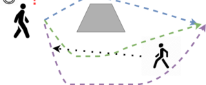
Figure 1: Illustration of a scenario where there are multiple ways that two pedestrians can avoid a collision. We present a method that given the same observed past, predicts multiple socially acceptable trajectories in crowded scenes.

The objective of this work is to develop a prediction model suitable for interaction-aware autonomous navigation. Hence, we address these limitations with a novel generative model for multi-modal trajectory prediction based on Variational Recurrent Neural Networks (VRNNs) [9]. We treat the multi-modal trajectory prediction problem as modeling the joint probability distribution over sequences.

This paper’s main contribution is a new interaction-aware variational recurrent neural network (Social-VRNN) design for one-shot multi-modal trajectory prediction. By following a variational approach, our method achieves faster convergence in comparison with GAN -based approach. Moreover, employing a time-dependent prior over the latent space enables our model to achieve state-of-the-art performance and generate diverse trajectories with a single network query.

To this end, we propose a training strategy to learn more diverse trajectories in an interpretable fashion. Finally, we present experimental results demonstrating that our method outperforms the state-of-the-art methods on both simulated and real datasets using one-shot predictions.

2 Related Works

Early works on human motion prediction are typically model-based. In [10], a model of human-human interactions was proposed by simulating attractive and repulsive physical forces denominated as social forces. To account for human-robot interaction, a Bayesian model based on agent-based velocity space was proposed in [11]. However, these approaches do not capture the multi-hypothesis behavior of the human motion. To accomplish that, [12] proposed a path prediction model based on Gaussian Processes, known as interactive Gaussian Processes (IGP). This was done by modeling each individual’s path with a Gaussian Process. The main drawbacks of this approach are the usage of hand-crafted functions to model interaction, limiting their ability to learn beyond the perceptible effects, and is computationally expensive.

Recently, Recurrent Neural Networks (RNNs) have been employed in trajectory prediction problems [13]. Building on RNNs, a hierarchical architecture was proposed in [14] and [4], which incorporated information about the surrounding environment and other agents, and performed better than previous models. Despite the high prediction accuracy demonstrated by these models, they are only able to predict the average behavior of the pedestrians.

In contrast, Social LSTM [15] models the prediction state as a Bivariate Gaussian and thus, uncertainty can be incorporated. Moreover, interaction is modeled by changing the hidden state of each agent network according to the distance between the agents, a mechanism know as ”Social pooling”. Several approaches extended the latter either by incorporating other sources of information or proposing updates in the model architecture improving the performance of the model. For instance, head pose information from the other agents was incorporated in [16] resulting in a significant increase of the prediction accuracy. Context information from visual images was used to encode both human-human and human-space interactions [17]. Social pooling has been extended to generate collision-free predictions [18] and to preserve spatial information by employing Grid LSTMs [19].

However, previous approaches did not consider the inherent multi-modal nature of human motions. In [7], a generative model based on Generative Adversarial Networks (GANs) was developed to generate multi-modal predictions by randomly sampling from the latent space. This approach was extended with two attention mechanisms to incorporate information from scene context and social interactions [20]. However, GANs are very susceptible to mode collapsing causing these models to generate very similar trajectories. To avoid mode collapse, a recently improved Info-GAN for multi-modal trajectory prediction was proposed [8]. Besides, [21] proposed a different training strategy to overcome the latter issue and improve trajectory prediction diversity. To account for the environment constraints, [22] proposed to include scene context information provided by a top-view camera of the scene. However, such information is not available in a real autonomous navigation scenario. Moreover, to improve social interaction modelling, Graph Neural Networks have been used in [23, 24]. Nonetheless, GANs are very difficult to train and typically require a large number of iterations until it converges to a stable Nash equilibrium.

Similar to our approach, the Trajectron++ [25] employs variational learning to improve training convergence and speed. Kernel-based methods employed Mixture Density Networks (MDNs) to build a continuous map capturing the possible motion directions [26] or to learn a multi-model distribution over a set of trajectories [27]. Nevertheless, [28] assumes a time-independent prior over the latent space, and [26, 27] requires a large number of samples to produce distinct trajectories. In contrast, we propose a novel architecture to learn a multi-modal prediction model based on VRNNs that can significantly improve the network prediction performance and diversity. Moreover, our method only uses local information enabling its application for autonomous navigation.

3 Variational Recurrent Neural Network

In this section, we present our Variational Recurrent Neural Network (VRNN) for multi-modal trajectory prediction, depicted in Fig. 2.

3.1 Multi-modal Trajectory Prediction Problem Formulation

Consider a navigation scenario with $n$ interacting agents (pedestrians) navigating on a plane $\pazocal{W}=\mathbb{R}^{2}$. The dataset $\mathbf{D}$ contains information about the $i$-th pedestrian trajectory $\tau^{i}_{1:N}=\{(\mathbf{p}_{1}^{i},\mathbf{v}_{1}^{i}),\dots,(\mathbf{p}_{N}^{i},\mathbf{v}_{N}^{i})\}$ with $N$ utterances and their corresponding surrounding static environment $\pazocal{O}^{i}_{\textrm{env}}\subset\pazocal{W}$, for $i\in[0,\dots n]$. $\mathbf{v}^{i}_{t}=\{v^{i}_{x,t},v^{i}_{y,t}\}$ is the velocity and $\textbf{p}^{i}_{t}=\{p^{i}_{x,t},p^{i}_{y,t}\}$ is the position of the $i$-th pedestrian at time $t$ in the world frame. Without loss of generality, $t=0$ indicates the current time and $t=-1$ the previous time-step. $\mathbf{v}^{i}_{1:T_{H}}=(\mathbf{v}^{i}_{1},\dots,\mathbf{v}^{i}_{T_{H}})$ represents the future pedestrian velocities over a prediction horizon $T_{H}$ and $\mathbf{v}^{i}_{-T_{O}:0}$ the pedestrian past velocities within an observation time $T_{O}$. Throughout this paper the subscript $i$ denotes the query-agent, i.e., the agent that we want to predict its future motion, and $-i$ the collection of all the other agents. Bold symbols are used to represent vectors and the non bold $x$ and $y$ subscripts are used to refer to the x and y direction in the world frame. $\mathbf{x}^{i}_{0}=\{\mathbf{v}^{i}_{-T_{O}:0},\mathbf{p}^{-i}_{0},\pazocal{O}^{i}_{\textrm{env}}\}$ represents the query-agent current state information. To account for the uncertainty and multimodality of the $i$-th pedestrian’s motion, we seek a probabilistic model $f(\theta)$ with parameters $\theta$ over a set of $M$ different trajectories $\forall m\in[0,M]$:

$$\begin{array}[]{c}p(\mathbf{v}^{i,m}_{1:T_{H}}|\mathbf{x}^{i}_{0})=f(\mathbf{x}^{i}_{0},\theta)\end{array}$$ (1)

where $m$ is the trajectory index. The probability is conditional to other agents states and the surrounding environment to model the interaction and environment constraints.

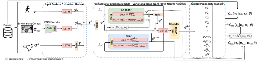
Figure 2: VRNN architecture for multi-modal trajectory prediction composed by: an input feature extraction, a probabilistic inference and output probability module. The first creates a joint representation of the input data $\mathbf{y}^{i}=\{\mathbf{y}^{i}_{\mathbf{v}},\mathbf{y}^{i}_{\textrm{env}},\mathbf{y}^{-i}\}$. The probabilistic inference module (Section 3.3) is based on the VRNN [9] incorporating: a encoder network to approximate a time-dependent posterior distribution $q(\mathbf{z}_{0}|\mathbf{x}_{\leq 0},\mathbf{z}_{<0})\sim\mathscr{N}(\mathbf{\mu}_{\mathbf{z},0},\textrm{diag}(\mathbf{\sigma}^{2}_{\mathbf{z},0}))$ with $[\mathbf{\mu}_{\mathbf{z},0},\mathbf{\sigma}_{\mathbf{z},0}]=\psi^{\textrm{enc}}(\psi^{\mathbf{x}}(\mathbf{x}_{0}),\mathbf{h}_{-1},\theta_{q})$ with $\theta_{q}$ as the approximate posterior model parameters; a decoder network to model the conditional generation distribution $\mathbf{\mathbf{v}}_{k}|\mathbf{x}_{0},\mathbf{z}_{0}\sim\mathscr{N}(\mathbf{\mu}_{\mathbf{x},0},\textrm{diag}(\mathbf{\sigma}^{2}_{\mathbf{x},0}))$ with $[\mathbf{\mu}_{\mathbf{v},1:T_{H}},\mathbf{\sigma}_{\mathbf{v},1:T_{H}}]=\psi^{\textrm{dec}}(\psi^{\mathbf{z}}(\mathbf{z}_{0}),\psi^{\mathbf{x}}_{t}(\mathbf{x}_{0}),\mathbf{h}_{-1},\theta_{\mathrm{dec}})$ with $\theta_{\mathrm{dec}}$ as the inference model parameters; a prior on the latent random variable $\mathbf{z}\sim\mathscr{N}(\mu_{\textrm{prior},0},\mathbf{\sigma}_{\textrm{prior},0})$ conditional to the hidden-state of the decoder network $[\mathbf{\mu}_{\textrm{prior},0},\mathbf{\sigma}_{\textrm{prior},0}]=\psi^{\textrm{prior}}(\mathbf{h}_{-1},\theta_{\textrm{prior}})$ with parameters $\theta_{\mathrm{prior}}$. Finally, the output probability module is a GMM (Section 3.4).

3.2 Input feature extraction module

This module creates a joint representation of three sources of information: the query-agent state, the environment context and social context. The first input is a sequence of $T_{O}$ history velocities $\mathbf{v}^{i}_{-T_{O}:0}$ of the query-agent. The second input is a local occupancy grid $O^{i}_{\textrm{env}}$, centered at the query-agent containing information about static obstacles (environment context) with width $D_{x}$ and height $D_{y}$. Here, we use the global map provided with publicly available datasets [29, 19]. In a real scenario, the map information can be obtained by building a map offline [30] or local map from online [31] using onboard sensors such as Lidar. Due to its high dimensionality, a convolution neural network (CNN) is used to obtain a compressed representation of this occupancy map while maintaining the spatial context. The encoder parameters are obtained by pre-training an Encoder-Decoder structure to minimize $\mathscr{L}_{\textrm{env}}=\sum^{D_{x}}_{i=1}\sum^{D_{y}}_{j=1}(\hat{\mathbf{O}^{i}_{\textrm{env}}}-\mathbf{O}^{i}_{\textrm{env}})^{2}$, as proposed in [4]. In addition, an LSTM layer is added to the first two input channels, modeling the existing time-dependencies.

The third input provides information about the interaction among the pedestrians containing information about their relative dynamics and spatial configuration. More specifically, it is a vector $\mathbf{O}^{-i}_{0}=[\mathbf{p}_{0}^{-1}-\mathbf{p}_{0}^{i},\mathbf{v}_{0}^{-1}-\mathbf{v}_{0}^{i},\dots\mathbf{p}_{0}^{-n}-\mathbf{p}_{0}^{i},\mathbf{v}_{0}^{-n}-\mathbf{v}_{0}^{i}]$ with the positions and velocities of the surrounding pedestrians relative to the query-agent. This input vector is then fed into an LSTM, allowing to create a fixed-size representation of the query’s agent social context and to consider a variable number of surrounding pedestrians. Finally, the outputs of each channel are concatenated creating a compressed and time-dependent representation of the input data $\mathbf{y}^{i}=\{\mathbf{y}^{i}_{\mathbf{v}},\mathbf{y}^{i}_{\textrm{env}},\mathbf{y}^{-i}\}$. Note that we only use past information about the query-agent velocities. For the other inputs only the current information is used.

3.3 Probabilistic Inference Module

The probabilistic inference module is based on the structure of the VRNN, as depicted in Fig. 2. It contains three main components: a prior model, a encoder model and decoder model. We use a fully connected layer (FCL) with Relu activation as the encoder model $\psi^{\textrm{enc}}$, the feature extractor of the joint input $\psi^{\mathbf{x}}$ and of the latent random variables $\psi^{\mathbf{z}}$, and the representation of the prior distribution $\psi^{\textrm{prior}}$. $\{\theta_{\textrm{enc}},\theta_{\mathbf{x}},\theta_{\mathbf{z}},\theta_{\textrm{prior}}\}$ are the network parameters of $\{\psi^{\textrm{enc}},\psi^{\mathbf{x}},\psi^{\mathbf{z}},\psi^{\textrm{prior}}\}$, respectively. The output vectors $\{\psi^{\textrm{enc}}_{\tau},\psi^{\textrm{prior}}\}$ are then used to model the approximate posterior and prior distribution. We split the output vectors into two parts to model the mean and variance, as represented in Fig. 2, and apply the following transformations to ensure a valid predicted distribution: $[\mu_{\mathrm{prior}},\mu_{\mathbf{z}}]=[\psi^{\textrm{prior}}_{1:w_{\textrm{prior}}},\psi^{\textrm{enc}}_{1:w_{\mathbf{z}}}]$ and $[\sigma_{\textrm{prior}},\sigma_{\mathbf{z}}]=[\exp{\psi^{\textrm{prior}}_{w_{\textrm{prior}}:2w_{\textrm{prior}}}},\exp{\psi^{\mathbf{z}}_{w_{\mathbf{z}}:2w_{\mathbf{z}}}}]$. $2w_{\textrm{prior}}$ and $2w_{\mathbf{z}}$ are the output vector size of the prior and latent random variable, respectively. This ensures that the standard deviation is always positive. Furthermore, we employ a LSTM layer as the RNN model propagating the hidden-state for the prior model and encoding the time-dependencies for the generative model. In contrast to [9] our generation model conditionally depends on the previous inputs:

$$\begin{split}&\mathbf{\mathbf{v}}_{k}|\mathbf{x}_{0},\mathbf{z}_{0}\sim\mathscr{N}(\mathbf{\mu}_{\mathbf{v},k},\textrm{diag}(\mathbf{\sigma}^{2}_{\mathbf{v},k}))\\ &[\mathbf{\mu}_{\mathbf{v},k},\mathbf{\sigma}_{\mathbf{v},k}]=\psi^{\textrm{dec}}(\psi^{\mathbf{z}}(\mathbf{z}_{0}),\psi^{\mathbf{x}}(\mathbf{y}^{i}_{0}),\mathbf{h}_{-1})\\ \end{split}$$ (2)

Lastly, the decoder model consists of two FC layers, with ELU [32] and linear activation, directly connected to the output of the LSTM network. Our models outputs in one shot $T_{H}$ steps considering the compressed and time-dependent input representation $\mathbf{y}^{i}_{0}$.

3.4 Multi-modal Trajectory Prediction Distribution

To predict one-shot multi-modal trajectories,we model the output of our network as a Gaussian Mixture Model (GMM), similar to [33] and [34], with $M>1$ modes accounting for the multimodality of the pedestrian’s motion. For each mode $m\in\{1,\dots,M\}$, we predict a sequence of future pedestrian velocities $v^{i,m}_{1:T_{H}}$ represented by a bivariate Gaussian $v^{i,m}_{k}\sim\mathscr{N}(\mu^{i,m}_{x,k},\mu^{i,m}_{y,k},\sigma^{i,m}_{x,k},\sigma^{i,m}_{y,k}),k=1,2,\dots,T_{H}$, capturing its motion uncertainty. Consequently, a modal trajectory is defined as a sequence of independent bivariate Gaussian’s with length $T_{H}$. The $M$ modes represent a set of $M$ possible trajectories resulting in the following probabilistic model:

$$p(\mathbf{v}^{i}_{k}|\mathbf{x}_{0},\mathbf{z}_{0},\mathbf{h}_{0},\mathbf{\theta})=\sum_{m=1}^{M}\pi_{m}p_{G}(\mathbf{\mu}^{i}_{k,m},\mathbf{\sigma}^{i}_{k,m})$$ (3)

where $p_{G}$ is the probability density function of multivariate Gaussian distributions, $\mathbf{\theta}=\{\theta_{\textrm{enc}},\theta_{\textrm{dec}},\theta_{\mathbf{x}},\theta_{\mathbf{z}},\theta_{\textrm{prior}}\}$ are the model parameters, $\mathbf{\mu}^{i,m}_{k}=[\mathbf{\mu}^{i,m}_{x,k},\mathbf{\mu}^{i,m}_{y,k}]$ and $\mathbf{\sigma}^{i,m}_{k}=[\mathbf{\sigma}^{i,m}_{x,k},\mathbf{\sigma}^{i,m}_{y,k}]$ are the mean and standard deviation of the predicted velocity vectors for the $m$-th predicted trajectory with likelihood $\pi_{m}$ at time-step $k$, respectively. The transformations described in Sec.3.3 and Fig.2 are applied to the network outputs $\psi^{\textrm{dec}}_{\tau}$ to ensure a valid distribution parametrization.

3.5 Improving Diversity

Generative models have the key advantage of allowing to perform inference by randomly sampling the latent random variable $\mathbf{z}$ from some prior distribution. Here, we propose a strategy to induce our model to learn a more “diverse” distribution of trajectories in a interpretable fashion, similar to [35]. Our VRNN models a generative distribution conditionally dependent on the input representation vector $\mathbf{\mathbf{y}^{i}}$, which is composed by three sub-vectors $\{\mathbf{y}^{i}_{\mathbf{v}},\mathbf{y}^{i}_{\textrm{env}},\mathbf{y}^{-i}\}$. Now, let’s assume that each input vector is a random variable with the following distribution:

$$\mathbf{y}^{i}_{\mathbf{v}}\sim\mathscr{N}(\mathbf{y}^{i}_{0,\mathbf{v}},\sigma_{\mathbf{v}})$$ (4)

$$\mathbf{y}^{i}_{\textrm{env}}\sim\mathscr{N}(\mathbf{y}^{i}_{0,\textrm{env}},\sigma_{\textrm{env}})$$ (5)

$$\mathbf{y}^{-i}\sim\mathscr{N}(\mathbf{y}^{-i}_{0},\sigma_{-i})$$ (6)

where $\{\mathbf{y}^{i}_{\mathbf{v}},\mathbf{y}^{i}_{\textrm{env}},\mathbf{y}^{-i}\}$ are random variables representing the variability of the agent state, the environment and surrounding agents context, respectively. $\{\sigma_{\mathbf{v}},\sigma_{\textrm{env}},\sigma_{-i}\}$ are the variance of each input channel and are considered as hyperparameters of our model. Hence, by sampling from these input distributions we can condition the generation distribution of $\mathbf{x}$ according with the uncertainty on the pedestrian state or the environment context and generate different trajectories $\tilde{\mathbf{v}}^{i}_{1:T_{H}}$ by varying the pedestrian conditions. Then, we introduce a loss function which motivates our model to cover the generated trajectories as the following cross-entropy term:

$$\mathscr{L}_{div}=\sum_{m=1}^{M}\sum_{k=1}^{T_{H}}-\mathbb{E}[\log p_{G}(\mathbf{\tilde{v}}_{k}|\mathbf{x}_{0},\mathbf{z}_{0})]$$ (7)

where $\mathbf{\tilde{v}}_{m,k}$ is a velocity sample at time-step $k$ from the m-th sampled trajectory.

3.6 Training Procedure

The model is trained end-to-end except for the CNN which is pre-trained. We train it using back-propagation through time (BTTP) with fixed truncation depth $t_{\textrm{trunc}}$. Furthermore, we apply the reparametrization trick [36] to obtain a continuous differentiable sampler and train the network using backpropagation. We learn the data distribution by minimizing a timestep-wise variational lower bound with annealing KL-Divergence as loss function [37]:

$$\mathscr{L}=\mathscr{L}_{m}+\lambda*(\mathscr{L}_{\textit{KL}}+\mathscr{L}_{div})$$ (8a)

$$\mathscr{L}_{m}=\sum_{m=1}^{M}\sum_{k=1}^{T_{H}}-\mathbb{E}_{\mathbf{x}_{0}\sim\mathbf{D}}[\log\pi_{m}p_{G}(\mathbf{v}_{k}|\mathbf{z}_{0},\mathbf{x}_{0})]$$ (8b)

$$\mathscr{L}_{\textit{KL}}(\mathbf{z}_{0}|\mathbf{x}_{\leq 0},\mathbf{z}_{<0})=\lambda\text{KL}(q(\mathbf{z}_{0}|\mathbf{x}_{\leq 0},\mathbf{z}_{<0})||p_{G}(\mathbf{z}_{0}|\mathbf{x}_{<0},\mathbf{z}_{<0}))$$ (8c)

where $\lambda$ is the annealing coefficient.

The first term represents the reconstruction loss (Eq. 8b) and the second the KL-Divergence between the approximated posterior $q(\textbf{z}_{0}|\textbf{x}_{\leq 0},\textbf{z}_{<0})$ (Eq. 8c) and the prior distribution of $\mathbf{z}$. Here, the prior over the latent random variable $\mathbf{z}$ is chosen to be a simple Gaussian distribution with mean and variance $[\mathbf{\mu}_{\textrm{prior},0},\mathbf{\sigma}_{\textrm{prior},0}]=\psi^{\textrm{prior}}(\mathbf{h}_{-1})$ depending on the previous hidden state. During training we aim to find the model parameters which minimize the loss function presented in Equation 8a. The annealing coefficient allows the model first to learn the parameters that fit the data well and later in the training phase to match the prior distribution and improve the diversity of the predicted trajectories.

4 Experiments

In this section, we show the obtained results of our generative model for simulation and real data. We present a qualitative analysis and performance results of our method against three baselines. To evaluate the performance of our model against the proposed baselines we use the following evaluation metrics: the average displacement error (ADE) and the final displacement error (FDE). The first two assess the prediction performance. For the models outputting probability distributions, the mean values are used to compute the ADE and FDE metrics. For the multi-modal distributions, we use the trajectory with the minimum error as in [8].

4.1 Experimental Settings

We trained our model using RMSProp [38] which is known to perform well in non-stationary problems with a initial learning rate $\alpha=10^{-4}$ exponentially decaying at a rate of 0.9 and a mini-batch size of 16. We used a KL annealing coefficient $\lambda=\tanh(\frac{\textrm{step}-10^{4}}{10^{3}})$, with step as the training step. We set the diversity weight $\beta$ to 0.2 and $\{\sigma_{\mathbf{x}^{v}},\sigma_{\mathbf{x}^{\textrm{env}}},\sigma_{\mathbf{x}^{-i}}\}=\{0.2,0.2,0\}$. Additionally, to avoid gradient explosion we clip the gradients to 1.0. We trained and evaluated our model for different prior, latent random variable and input feature vector sizes. The configuration achieving lower validation error was $\{128,128,512\}$, for the prior, latent random variable and input feature vector size, respectively. Moreover, we use $M=3$ mixture components for the models using a GMM as the output function. We set $T_{H}=12$ prediction steps corresponding to 4.8 s of prediction horizon and $T_{O}=8$ as used in previous methods [8, 20]. The models were implemented using Tensorflow [39] and were trained on a NVIDIA GeForce GTX 980 requiring $2\times 10^{4}$ training steps, or approximately 2 hours. The simulation datasets were obtained with the open-source ROS implementation of the Social Forces model [10]. Our VRNN will be released open source.

4.2 Performance evaluation

We compared our model with the following state-of-art prediction baselines:

• LSTM-D [4]: A deterministic interaction-aware model, incorporating the interaction between the agents and static obstacles.

• SoPhie [20]: a GAN model implementing a Social and Physical attention mechanism.

• Social-ways (S-Ways) [8]: The state-of-art GAN based method for multi-modal trajectory prediction.

• STORN [40]: Our VRNN model considering a time-independent prior as a Gaussian distribution with zero mean and unit variance.

Table 1: Performance results of our proposed method (VRNN) vs. baselines. The results presented for the Social Ways with 30 samples ($K=30$) and SoPhie method were taken from [15] and [20], respectively. The ADE and FDE values are separated by slash. The average values (AVG) only consider the results for the real datasets. The results for using three samples ($K=3$) of S-Ways were obtained from the open-source implementation provided by [8].

	Deterministic	Stochastic
	Single Sample	Multiple Samples			Single Sample
Dataset	LSTM	SoPhie	S-Ways ($K=30$)	S-Ways ($K=3$)	STORN	VRNN
ETH	0.40 / 0.65	0.70 / 1.43	0.39 / 0.64	0.78 / 1.48	0.73 / 1.49	0.39 / 0.70
Hotel	0.45 / 0.75	0.76 / 1.67	0.39 / 0.64	0.53 / 0.95	1.33 / 1.45	0.35 / 0.47
Univ	1.02 / 1.54	0.54 / 1.24	0.55 / 1.31	0.81 / 1.53	0.82 / 1.17	0.53 / 0.65
ZARA01	0.35 / 0.68	0.30 / 0.63	0.44 / 0.64	0.87 / 1.30	0.91 / 1.52	0.41 / 0.70
ZARA02	0.54 / 0.92	0.38 / 0.78	0.51 / 0.92	1.27 / 2.13	0.91 / 1.52	0.51 / 0.55
AVG	0.55 / 0.90	0.54 / 1.15	0.46 / 0.83	0.86 / 1.47	0.94 / 1.43	0.44 / 0.61

We use the open-source implementation of [8] to obtain the results for S-Ways considering only 3 samples $(K=3)$ as the number of trajectories predicted by our method and as suggested in [41]. We adopt the same dataset split setting as in [8] using 4 sets for training and the remaining set for testing. Aggregated results in Table 1 show that our method outperformed the deterministic baselines, STORN, and S-Ways using three samples. Moreover, the results show that our method achieves comparable performance with state-of-the-art methods using a high number of samples on the Zara01, Zara02 and ETH datasets. In contrast, our method achieves the best performance on the Hotel and Univ datasets. Finally, the poor performance of the STORN model results show that employing a time-dependent prior improves the prediction performance significantly.

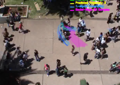
Figure 3: Social-VRNN predicted trajectories vs a multi-modal prediction baseline, Social-Ways [8]. In blue is depicted the ground truth trajectory, in red, green and yellow the three possible predicted trajectories by our model, in light blue the one sigma boundary of the predicted trajectory and, in magenta 30 sampled predicted trajectories by the Social-Ways model.

4.3 Qualitative analysis

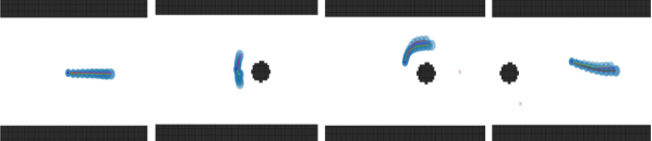
a) In this scenario, one agent is moving along a corridor with an obstacle in the middle. The agent is moving from the left to the right. When she finds the obstacle in the middle of its path, our model successfully predicts two hypotheses: going left or right. Once she is already avoiding the obstacle through the left side, the model predicts three hypotheses for the pedestrian to continue its collision avoidance maneuver, with varying clearance levels. Finally, when she is in free space all the predicted trajectories collapse to a single-mode.

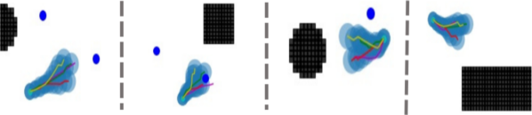
b) This sub-figure illustrates four sample results obtained in a more complex simulated scenario, with several static obstacles and 15 agents. The two left figures show two situations where the agent can avoid another agent on its left, right or by simply move straight because the other will keep moving away. The two right figures show the ability of our model to predict different trajectories that an agent may follow to avoid a static obstacle.

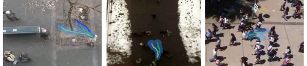
c) Three examples of multi-modal trajectory prediction using our model in real scenarios. In blue is depicted the ground truth trajectory, in red, green and yellow the three possible predicted trajectories, in light blue the one sigma boundary of the predicted trajectory.

Figure 4: The scenarios depicted in Fig.4(a) and (b) were simulated by using the Social Forces model [10] for the pedestrians. In magenta the real trajectory, in red, green and yellow the mean values of each trajectory hypothesis and, in blue the 1-$\sigma$ uncertainty boundaries of each trajectory. The dark blue dots represent the other agents. The plotted trajectories correspond to a single network query.

In this section we present prediction results for simulated and real scenarios, as depicted in Fig. 4. We have created two datasets to demonstrate this multi-modal behavior with static obstacles (Fig.4(a)), and other pedestrians (Fig. 4(b)). Figure 4(a) shows the ability of our method to predict different trajectories according to the environment structure. Figure 4(b) demonstrates that our method can scale to more complex environments, with several pedestrians and obstacles, and predict different motion hypotheses.

Moreover, we evaluate our method on real data using the publicly available datasets [29, 19]. In Fig. 4(c) on the left, our model infers two possible trajectories for the pedestrian to avoid a tree. In addition, in the central and right images of Fig. 4(c), our model predicts two possible trajectories to move through the crowd. Finally, Fig. 3 shows predicted trajectories for both Social-VRNN and Social-Ways model in a crowded scene. The predicted trajectories from the Social-VRNN model can capture two distinct trajectories through the crowd. In contrast, Social-Ways only captures one mode, even considering 30 samples from the baseline model. The presented results demonstrate that our model can effectively infer different trajectories according to the environment and social constraints from a single query. We refer the reader to the video accompanying this article for more details on the presented results.

5 CONCLUSION

In this paper, we introduced a Variational Recurrent Neural Network (VRNN) architecture for multi-modal trajectory prediction in one-shot and considering the pedestrian dynamics, interactions among pedestrians and static obstacles. Building on a variational approach and learning a mixture Gaussian model enables our model to generate distinct trajectories accounting for the static obstacles and the surrounding pedestrians. Our approach allows us to improve the state-of-the-art prediction performance in scenarios with a large number of agents (e.g., Univ dataset) or containing static obstacles (e.g., Hotel dataset) from a single prediction shot. Furthermore, the proposed approach reduces significantly the number of samples needed to achieve good prediction with high accuracy. As future work, we aim to integrate the proposed method with a real-time motion planner on a mobile platform for autonomous navigation among pedestrians.

Acknowledgments

This work was supported by the Amsterdam Institute for Advanced Metropolitan Solutions and the Netherlands Organisation for Scientific Research (NWO) domain Applied Sciences (Veni 15916).

References

- Brito et al. [2019] B. Brito, B. Floor, L. Ferranti, and J. Alonso-Mora. Model predictive contouring control for collision avoidance in unstructured dynamic environments. IEEE Robotics and Automation Letters, 4(4):4459–4466, 2019.
- Lin et al. [2020] J. Lin, H. Zhu, and J. Alonso-Mora. Robust vision-based obstacle avoidance for micro aerial vehicles in dynamic environments. In 2020 IEEE International Conference on Robotics and Automation (ICRA), pages 2682–2688. IEEE, 2020.
- Kothari et al. [2020] P. Kothari, S. Kreiss, and A. Alahi. Human trajectory forecasting in crowds: A deep learning perspective. arXiv preprint arXiv:2007.03639, 2020.
- Pfeiffer et al. [2018] M. Pfeiffer, G. Paolo, H. Sommer, J. Nieto, R. Siegwart, and C. Cadena. A data-driven model for interaction-aware pedestrian motion prediction in object cluttered environments. In 2018 IEEE International Conference on Robotics and Automation (ICRA), pages 1–8. IEEE, 2018.
- Lötjens et al. [2019] B. Lötjens, M. Everett, and J. P. How. Safe reinforcement learning with model uncertainty estimates. In 2019 International Conference on Robotics and Automation (ICRA), pages 8662–8668. IEEE, 2019.
- Gal and Ghahramani [2016] Y. Gal and Z. Ghahramani. Dropout as a bayesian approximation: Representing model uncertainty in deep learning. In international conference on machine learning, pages 1050–1059, 2016.
- Gupta et al. [2018] A. Gupta, J. Johnson, L. Fei-Fei, S. Savarese, and A. Alahi. Social gan: Socially acceptable trajectories with generative adversarial networks. In Proceedings of the IEEE Conference on Computer Vision and Pattern Recognition, pages 2255–2264, 2018.
- Amirian et al. [2019] J. Amirian, J.-B. Hayet, and J. Pettré. Social ways: Learning multi-modal distributions of pedestrian trajectories with gans. In Proceedings of the IEEE Conference on Computer Vision and Pattern Recognition Workshops, pages 0–0, 2019.
- Chung et al. [2015] J. Chung, K. Kastner, L. Dinh, K. Goel, A. C. Courville, and Y. Bengio. A recurrent latent variable model for sequential data. In Advances in neural information processing systems, pages 2980–2988, 2015.
- Helbing and Molnar [1995] D. Helbing and P. Molnar. Social force model for pedestrian dynamics, 1995. ISSN 1063651X.
- Kim et al. [2015] S. Kim, S. J. Guy, W. Liu, D. Wilkie, R. W. Lau, M. C. Lin, and D. Manocha. BRVO: Predicting pedestrian trajectories using velocity-space reasoning. International Journal of Robotics Research, 34(2):201–217, 2015. ISSN 17413176.
- Trautman and Krause [2010] P. Trautman and A. Krause. Unfreezing the robot: Navigation in dense, interacting crowds. In IEEE/RSJ 2010 International Conference on Intelligent Robots and Systems, IROS 2010 - Conference Proceedings, pages 797–803, 2010. ISBN 9781424466757.
- Becker et al. [2018] S. Becker, R. Hug, and M. Arens. An Evaluation of Trajectory Prediction Approaches and Notes on the TrajNet Benchmark. 2018.
- Xue et al. [2018] H. Xue, D. Q. Huynh, and M. Reynolds. Ss-lstm: A hierarchical lstm model for pedestrian trajectory prediction. In 2018 IEEE Winter Conference on Applications of Computer Vision (WACV), pages 1186–1194. IEEE, 2018.
- Alahi et al. [2016] A. Alahi, K. Goel, V. Ramanathan, A. Robicquet, L. Fei-Fei, and S. Savarese. Social lstm: Human trajectory prediction in crowded spaces. In Proceedings of the IEEE Conference on Computer Vision and Pattern Recognition, pages 961–971, 2016.
- Hasan et al. [2018] I. Hasan, F. Setti, T. Tsesmelis, A. Del Bue, F. Galasso, and M. Cristani. Mx-lstm: mixing tracklets and vislets to jointly forecast trajectories and head poses. In Proceedings of the IEEE Conference on Computer Vision and Pattern Recognition, pages 6067–6076, 2018.
- Bartoli et al. [2018] F. Bartoli, G. Lisanti, L. Ballan, and A. Del Bimbo. Context-aware trajectory prediction. In 2018 24th International Conference on Pattern Recognition (ICPR), pages 1941–1946. IEEE, 2018.
- Xu et al. [2018] K. Xu, Z. Qin, G. Wang, K. Huang, S. Ye, and H. Zhang. Collision-free lstm for human trajectory prediction. In International Conference on Multimedia Modeling, pages 106–116. Springer, 2018.
- Lerner et al. [2007] A. Lerner, Y. Chrysanthou, and D. Lischinski. Crowds by example. In Computer graphics forum, volume 26, pages 655–664. Wiley Online Library, 2007.
- Sadeghian et al. [2019] A. Sadeghian, V. Kosaraju, A. Sadeghian, N. Hirose, H. Rezatofighi, and S. Savarese. Sophie: An attentive gan for predicting paths compliant to social and physical constraints. In Proceedings of the IEEE Conference on Computer Vision and Pattern Recognition, pages 1349–1358, 2019.
- Makansi et al. [2019] O. Makansi, E. Ilg, O. Cicek, and T. Brox. Overcoming limitations of mixture density networks: A sampling and fitting framework for multimodal future prediction. In Proceedings of the IEEE Conference on Computer Vision and Pattern Recognition, pages 7144–7153, 2019.
- Zhao et al. [2019] T. Zhao, Y. Xu, M. Monfort, W. Choi, C. Baker, Y. Zhao, Y. Wang, and Y. N. Wu. Multi-agent tensor fusion for contextual trajectory prediction. In Proceedings of the IEEE Conference on Computer Vision and Pattern Recognition, pages 12126–12134, 2019.
- Chandra et al. [2020] R. Chandra, T. Guan, S. Panuganti, T. Mittal, U. Bhattacharya, A. Bera, and D. Manocha. Forecasting trajectory and behavior of road-agents using spectral clustering in graph-lstms. IEEE Robotics and Automation Letters, 5(3):4882–4890, 2020.
- Eiffert et al. [2020] S. Eiffert, K. Li, M. Shan, S. Worrall, S. Sukkarieh, and E. Nebot. Probabilistic crowd gan: Multimodal pedestrian trajectory prediction using a graph vehicle-pedestrian attention network. IEEE Robotics and Automation Letters, 5(4):5026–5033, 2020.
- Salzmann et al. [2020] T. Salzmann, B. Ivanovic, P. Chakravarty, and M. Pavone. Trajectron++: Dynamically-feasible trajectory forecasting with heterogeneous data. arXiv preprint arXiv:2001.03093, 2020.
- Zhi et al. [2019] W. Zhi, R. Senanayake, L. Ott, and F. Ramos. Spatiotemporal learning of directional uncertainty in urban environments with kernel recurrent mixture density networks. IEEE Robotics and Automation Letters, 4(4):4306–4313, 2019.
- Zhi et al. [2020] W. Zhi, L. Ott, and F. Ramos. Kernel trajectory maps for multi-modal probabilistic motion prediction. In Conference on Robot Learning, pages 1405–1414, 2020.
- Ivanovic and Pavone [2019] B. Ivanovic and M. Pavone. The trajectron: Probabilistic multi-agent trajectory modeling with dynamic spatiotemporal graphs. pages 2375–2384, 10 2019.
- Pellegrini et al. [2009] S. Pellegrini, A. Ess, K. Schindler, and L. Van Gool. You’ll never walk alone: Modeling social behavior for multi-target tracking. In 2009 IEEE 12th International Conference on Computer Vision, pages 261–268. IEEE, 2009.
- Zaman et al. [2011] S. Zaman, W. Slany, and G. Steinbauer. Ros-based mapping, localization and autonomous navigation using a pioneer 3-dx robot and their relevant issues. In 2011 Saudi International Electronics, Communications and Photonics Conference (SIECPC), pages 1–5. IEEE, 2011.
- Huang et al. [2005] G. Q. Huang, A. B. Rad, and Y. K. Wong. Online slam in dynamic environments. In ICAR ’05. Proceedings., 12th International Conference on Advanced Robotics, 2005., pages 262–267, 2005.
- Clevert et al. [2015] D.-A. Clevert, T. Unterthiner, and S. Hochreiter. Fast and accurate deep network learning by exponential linear units (elus). CoRR, abs/1511.07289, 2015.
- Bishop [1994] C. M. Bishop. Mixture density networks. Technical report, Citeseer, 1994.
- Graves [2013] A. Graves. Generating sequences with recurrent neural networks, 2013.
- Rhinehart et al. [2018] N. Rhinehart, K. M. Kitani, and P. Vernaza. R2p2: A reparameterized pushforward policy for diverse, precise generative path forecasting. In Proceedings of the European Conference on Computer Vision (ECCV), pages 772–788, 2018.
- Kingma and Welling [2013] D. P. Kingma and M. Welling. Auto-encoding variational bayes. CoRR, abs/1312.6114, 2013.
- Bowman et al. [2016] S. R. Bowman, L. Vilnis, O. Vinyals, A. Dai, R. Jozefowicz, and S. Bengio. Generating sentences from a continuous space. Proceedings of The 20th SIGNLL Conference on Computational Natural Language Learning, 2016. URL http://dx.doi.org/10.18653/v1/k16-1002.
- Tieleman and Hinton [2012] T. Tieleman and G. Hinton. Rmsprop: Divide the gradient by a running average of its recent magnitude. coursera: Neural networks for machine learning. Tech. Rep., Technical report, page 31, 2012.
- Abadi et al. [2015] M. Abadi, A. Agarwal, P. Barham, E. Brevdo, Z. Chen, C. Citro, G. S. Corrado, A. Davis, J. Dean, M. Devin, et al. Tensorflow: Large-scale machine learning on heterogeneous systems, 2015. Software available from tensorflow. org, 1(2), 2015.
- Bayer and Osendorfer [2014] J. Bayer and C. Osendorfer. Learning stochastic recurrent networks. arXiv preprint arXiv:1411.7610, 2014.
- [41] Trajnet++ (A Trajectory Forecasting Challenge). URL https://www.aicrowd.com/challenges/trajnet-a-trajectory-forecasting-challenge.