heightadjust=object \newfloatcommandcapbtabboxtable \newfloatcommandcapbfigboxfigure
Active Domain Adaptation via Clustering Uncertainty-weighted Embeddings
Abstract
Generalizing deep neural networks to new target domains is critical to their real-world utility. In practice, it may be feasible to get some target data labeled, but to be cost-effective it is desirable to select a maximally-informative subset via active learning (AL). We study the problem of AL under a domain shift, called Active Domain Adaptation (Active DA). We demonstrate how existing AL approaches based solely on model uncertainty or diversity sampling are less effective for Active DA. We propose Clustering Uncertainty-weighted Embeddings (CLUE), a novel label acquisition strategy for Active DA that performs uncertainty-weighted clustering to identify target instances for labeling that are both uncertain under the model and diverse in feature space. CLUE consistently outperforms competing label acquisition strategies for Active DA and AL across learning settings on 6 diverse domain shifts for image classification. Our code is available at https://github.com/virajprabhu/CLUE.
1 Introduction
Deep neural networks excel at learning from large labeled datasets but struggle to generalize to new target domains [39, 49]. This limits their real-world utility, as it is impractical to collect a large new dataset for every new deployment domain. Further, all target instances are usually not equally informative, and it is far more cost-effective to identify maximally informative target instances for labeling. While Active Learning [2, 7, 10, 12, 42, 43] has extensively studied the problem of identifying informative instances for labeling, it typically focuses on learning a model from scratch and does not operate under a domain shift. In many practical scenarios, models are trained in a source domain and deployed in a different target domain, often with additional domain adaptation [13, 21, 39, 51]. In this work, we study the problem of active learning under such a domain shift, called Active Domain Adaptation [36] (Active DA).
Concretely, given i) labeled data in a source domain, ii) unlabeled data in a target domain, and iii) the ability to obtain labels for a fixed budget of target instances, the goal of Active DA is to select target instances for labeling and learn a model with high accuracy on the target test set. Active DA has widespread utility as a means of cost-effective adaptation from cheaper to more expensive sources of labels (e.g. synthetic to real data), as well as when the quantity (e.g. autonomous driving) or cost (e.g. medical diagnosis) of labeling in the target domain is prohibitive. Despite its practical utility, it is a challenging task that has seen limited follow-up work since its introduction over ten years ago [5, 36, 47].
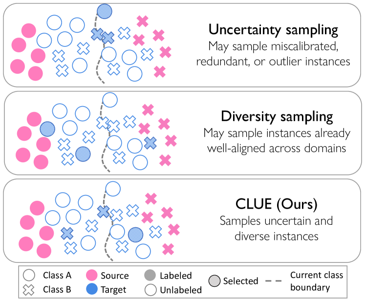
The traditional AL setting typically focuses on techniques to select samples to efficiently learn a model from scratch, rather than adapting under a domain shift [43]. As a result, existing state-of-the art AL methods based on either uncertainty or diversity sampling are less effective for Active DA. Uncertainty sampling selects instances that are highly uncertain under the model’s beliefs [12, 10, 48, 25]. Under a domain shift, uncertainty estimates on the target domain may be miscalibrated [46] and lead to sampling uninformative, outlier, or redundant instances (Fig. 1, top). A parallel line of work in AL based on diversity sampling instead selects instances dissimilar to one another in a learned embedding space [16, 42, 45]. In Active DA, this can lead to sampling uninformative instances from regions of the feature space that are already well-aligned across domains (Fig. 1, middle). As a result, solely using uncertainty or diversity sampling is suboptimal for Active DA, as we demonstrate in Sec 4.4.
Recent work in AL and Active DA has sought to combine uncertainty and diversity sampling. AADA [47], the state-of-the-art Active DA method, combines uncertainty with diversity measured by ‘targetness’ under a learned domain discriminator. However, targetness does not ensure that the selected instances are representative of the entire target data distribution (i.e. not outliers), or dissimilar to one another. Ash et al. [2] instead propose performing clustering in a hallucinated “gradient embedding” space. However, they rely on distance-based clustering in high-dimensional spaces, which often leads to suboptimal results.
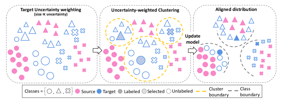
In this work, we propose a novel label acquisition strategy for Active DA that combines uncertainty and diversity sampling in a principled manner without the need for complex gradient or domain discriminator-based diversity measures. Our approach, Clustering Uncertainty-weighted Embeddings (CLUE), identifies informative and representative target instances from dense regions of the feature space. To do so, CLUE clusters deep embeddings of target instances weighted by the corresponding uncertainty of the target model. Our weighting scheme effectively increases the density of instances proportional to their uncertainty. To construct non-redundant batches, CLUE then selects nearest neighbors to the inferred cluster centroids for labeling. Our algorithm then leverages the acquired target labels and, optionally, the labeled source and unlabeled target data, to update the model, consistently leading to more cost-effective domain alignment than competing (and frequently more complex) alternatives.
Contributions:
-
1.
We benchmark the performance of state-of-the-art methods for active learning on challenging domain shifts, and find that methods based purely on uncertainty or diversity sampling are not effective for Active DA.
-
2.
We present CLUE, a novel and easy-to-implement label acquisition strategy for Active DA that uses uncertainty-weighted clustering to identify instances that are both uncertain under the model and diverse in feature space.
-
3.
We present results on 6 diverse domain shifts from the DomainNet [34], Office [39], and DIGITS [31, 27] benchmarks for image classification. Our method CLUE improves upon both the previous state-of-the art in Active DA across shifts (by as much as 9% in some cases), as well as state-of-the-art methods for active learning, across multiple learning strategies.
2 Related Work
Active Learning (AL) for CNN’s. AL for CNN’s has focused on the batch-mode setting due to the instability associated with single-instance updates. The two most successful paradigms in AL have been uncertainty sampling and diversity sampling [2]. Uncertainty-based methods select instances with the highest uncertainty under the current model [12, 10, 48, 41], using measures such as entropy [52], classification margins [37], or confidence. Diversity-based methods select instances that are representative of the entire dataset, and optimize for diversity in a learned embedding space, via clustering, or core-set selection [42, 16, 45, 15].
Some approaches combine these two paradigms [2, 3, 22, 56]. Active Learning by Learning [22] formulates this as a multi-armed bandit problem of selecting between coreset and uncertainty sampling at each step. Zhdanov et al. [56] use K-Means clustering [19] to increase batch diversity after pre-filtering based on uncertainty. More recently, BADGE [2] runs KMeans++ on hallucinated “gradient embeddings”. We propose CLUE, an AL method for sampling under a domain shift, that uses uncertainty-weighted clustering to select diverse and informative target instances.
Domain Adaptation. The task of transferring models trained on a labeled source domain to an unlabeled [39, 51, 13, 21] or partially-labeled [9, 54, 40] target domain has been studied extensively. Initial approaches aligned feature spaces by optimizing discrepancy statistics between the source and target [51, 28], while in recent years adversarial learning of a feature space encoder alongside a domain discriminator has become a popular alignment strategy [13, 14, 50]. In this work, we propose a label acquisition strategy for active learning under a domain shift that generalizes across multiple domain adaptation strategies.
Active Domain Adaptation (Active DA). Unlike semi-supervised domain adaptation which assumes labels for a random subset of target instances, Active DA focuses on selecting target instances to label for domain adaptation. Rai et al. [36] first studied the task of Active DA applied to sentiment classification from text data. They propose ALDA, which samples instances based on model uncertainty and a learned domain separator. Chattopadhyay et al. [5] select target instances and learn importance weights for source points by solving a convex optimization problem of minimizing MMD between features. More recently, Su et al. [47] study Active DA in the context of deep CNN’s and propose AADA, wherein target instances are selected based on predictive entropy and targetness measured by an adversarially trained domain discriminator, followed by adversarial domain adaptation via DANN [14]. We propose CLUE, a novel label acquisition strategy for Active DA that identifies uncertain and diverse instances for labeling that outperforms prior work on diverse shifts across multiple learning strategies.
3 Approach
We address active domain adaptation (Active DA), where the goal is to generalize a model trained on a source domain to an unlabeled target domain, with the option to query an oracle for labels for a subset of target instances. While individual facets of this task – adapting to a new domain and selective acquisition of labels, have been well-studied as the problems of Domain Adaptation (DA) and Active Learning (AL) respectively, Active DA presents the new challenge of identifying target instances that will, once labeled, result in the most sample-efficient domain alignment. Further, the answer to this question may vary based on the properties of the specific domain shift. In this section, we present CLUE, a novel label acquisition strategy for Active DA which performs consistently well across diverse domain shifts.
3.1 Notation & Preliminaries
In Active DA, the learning algorithm has access to labeled instances from the source domain (solid pink in Fig. 2), unlabeled instances from the target domain (blue outline in Fig. 2), and a budget ( in Fig. 2) which is much smaller than the amount of unlabeled target data. The learning algorithm may query an oracle to obtain labels for at most instances from , and add them to the set of labeled target instances . The entire target domain data is . The task is to learn a function (a convolutional neural network (CNN) parameterized by ) that achieves good predictive performance on the target. In this work, we consider Active DA in the context of -way image classification – the samples , are images, and labels , are categorical variables .
Active Learning. The goal of active learning (AL) is to identify target instances that, once labeled and used for training the model, minimize its expected future loss. In practice, prior works in AL identify such instances based primarily on two proxy measures, uncertainty and diversity (see Sec. 2). We first revisit these terms in the context of Active DA.
Uncertainty. Prior work in AL has proposed using several measures of model uncertainty as a proxy for informativeness (see Sec. 2). However, in the context of Active DA, using model uncertainty to select informative samples presents a conundrum. On the one hand, models benefit from initialization on a related source domain rather than learning from scratch. On the other hand, under a strong distribution shift, model uncertainty may often be miscalibrated [46]. Unfortunately however, without access to target labels, it is impossible to evaluate the reliability of model uncertainty!
Diversity. Acquiring labels solely based on uncertainty often leads to sampling batches of similar instances with high redundancy, or to sampling outliers. A parallel line of work in active learning instead proposes sampling diverse instances that are representative of the unlabeled pool of data. Several definitions of “diverse” exist in the literature: some works define diversity as coverage in feature [42] or “gradient embedding” space [2], while prior work in Active DA measures diversity by how “target-like” an instance is [47]. In Active DA, training on a related source domain (optionally followed by unsupervised domain alignment), results in some classes being better aligned across domains than others. Thus, in order to be cost-efficient it is important to avoid sampling from already well-learned regions of the feature space. However, purely diversity-based AL methods are unable to account for this, and lead to sampling redundant instances.
While sampling instances that are either uncertain or diverse may be useful to learning, an optimal label acquisition strategy for Active DA would ideally capture both jointly. We now introduce CLUE, a label acquisition strategy for Active DA that captures both uncertainty and diversity.
3.2 Clustering Uncertainty-weighted Embeddings
To measure informativeness we use predictive entropy [52] ( for brevity), which for -way classification, is defined as:
| (1) |
Under a domain shift, entropy can be viewed as capturing both uncertainty and domainness. Rather than training an explicit domain discriminator [13, 47], we consider an implicit domain classifier [40] based on entropy thresholding 111This assumes that source instances have low predictive entropy, which is generally satisfied under supervised training.:
| (2) |
where 1 and 0 denote target and source domain labels, and is a threshold value. The probability of an instance belonging to the target domain is thus given by:
| (3) |
where is the maximum possible entropy of a way distribution. Next, we measure diversity based on feature-space coverage. Let denote feature embeddings extracted from model . We identify diverse instances by partitioning into diverse sets via a partition function . Let denote the corresponding centroid of each set. Each set should have a small variance . Expressed in terms of pairs of samples, [55]. The goal is to group target instances that are similar in the CNN’s feature space, into a set . However, while is a function of the target data distribution and feature space , it does not account for uncertainty.
-
1.
Compute deep embedding
-
2.
Run Weighted K-Means until convergence (Eq. 4):
-
(a)
Init. (=B) centroids (KMeans++)
-
(b)
Assign:
-
(c)
Update:
-
(a)
-
3.
Acquire labels for nearest-neighbor to centroids
-
4.
To jointly capture both diversity and uncertainty, we propose weighting samples based on their uncertainty (given by Eq. 1), and compute the weighted population variance [35]. The overall set-partitioning objective is:
| (4) |
where the normalization . Our weighted set partitioning can also be viewed as standard set partitioning in an alternate feature space, where the density of instances is artificially increased proportional to their predictive entropy. Intuitively, this emphasizes representative sampling from uncertain regions of the feature space.
Since the objective in Eq. 4 is NP-hard, we approximate it using a Weighted K-Means algorithm [23] (see Algorithm 1 – uncertainty-weighting is used in the update step). We set (budget), and use activations from the penultimate CNN layer as . After clustering, to select representative instances (i.e. non-outliers), we acquire labels for the nearest neighbor to the weighted-mean of each set in Eq. 4. Note that Eq. 4 equivalently maximizes the sum of squared deviations between instances in different sets [26] , ensuring that the constructed batch of instances has minimum redundancy.
Trading-off uncertainty and diversity. CLUE captures an implicit tradeoff between model uncertainty (via entropy-weighting) and feature-space coverage (via clustering). Consider the predictive probability distribution for instance :
| (5) |
where denotes the softmax function and denotes its temperature. We observe that by modulating , we can control the uncertainty-diversity tradeoff. For example, by increasing , we obtain more diffuse softmax distributions for all points leading to similar uncertainty estimates across points; correspondingly, we expect diversity to play a bigger role. Similarly, at lower values of we expect uncertainty to have greater influence.
Our full label acquisition approach, Clustering Uncertainty-weighted Embeddings (CLUE), thus identifies instances that are both uncertain and diverse (see Fig. 2).
Domain adaptation. After acquiring labels via CLUE, we proceed to the next step of active adaptation: we update the model using the acquired target labels and optionally, the labeled source and unlabeled target data (see Fig. 2, right). In our main experiments (Sec. 4.4), we experiment with 3 learning strategies: i) finetuning on target labels, ii) domain-adversarial learning via DANN [13] with an additional target cross-entropy loss, and iii) semi-supervised adaptation via minimax entropy (MME [40]). In Sec 4.6 we also combine CLUE with additional DA methods from the literature.
Algorithm 1 describes our full approach when using CLUE in combination with semi-supervised domain adaptation. Given a model trained on labeled source instances, we align its representations with unlabeled target instances via unsupervised domain adaptation. For rounds with per-round budget , we iteratively i) acquire labels for target instances that are identified via our proposed sampling approach (CLUE), and ii) Update the model using a semi-supervised domain alignment strategy.
4 Experiments
We begin by describing our datasets and metrics, implementation details, and baselines (Sec 4.1- 4.3). Next, we benchmark the performance of CLUE across 6 domain shifts of varying difficulty against state-of-the art methods for Active DA and AL, across different learning settings (Sec 4.4). We then ablate our method, analyze its sensitivity to various hyperparameters, and visualize its behavior (Sec 4.5). Finally, we combine our method with various DA strategies, and study its effectiveness in learning from scratch (Sec 4.6). We follow the standard batch active learning setting [4], in which we perform multiple rounds of batch active sampling, label acquisition, and model updates.
4.1 Datasets and Metrics
DomainNet. DomainNet [34] is a large domain adaptation benchmark for image classification, containing 0.6 million images from 6 distinct domains spanning 345 categories. We study four shifts of increasing difficulty as measured by sourcetarget transfer accuracy (TA): RealClipart (easy, TA=40.6%), ClipartSketch (moderate, TA=34.7%), SketchPainting (hard, TA=30.3%), and ClipartQuickdraw (very hard, TA=11.9%).
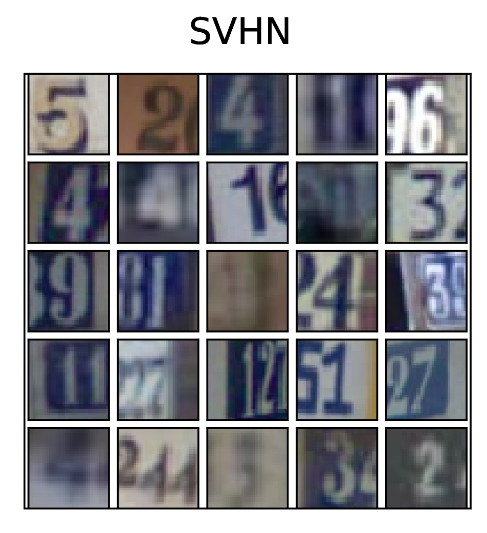
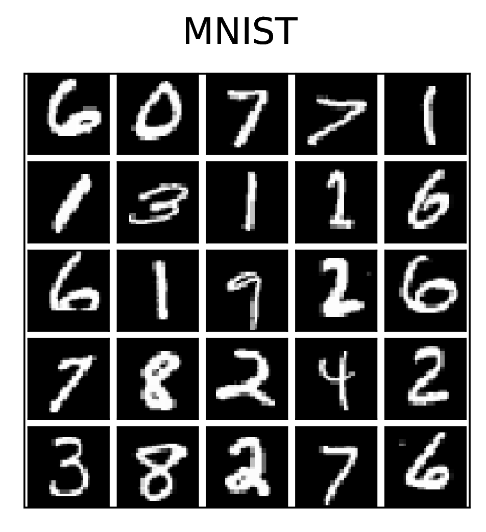
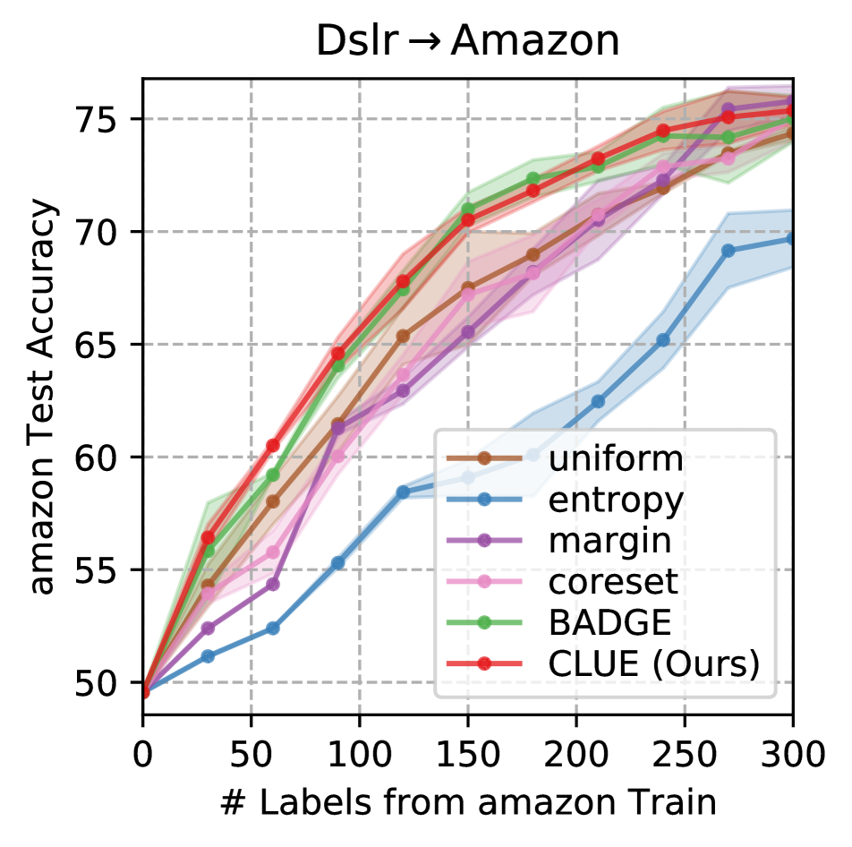
DIGITS and Office. We also report performance on the SVHN [31]MNIST [27] and DSLRAmazon [39] shifts.
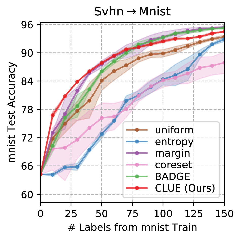
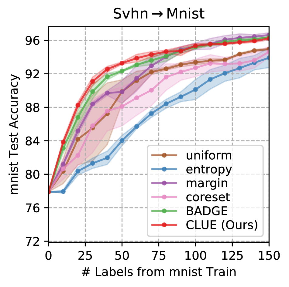
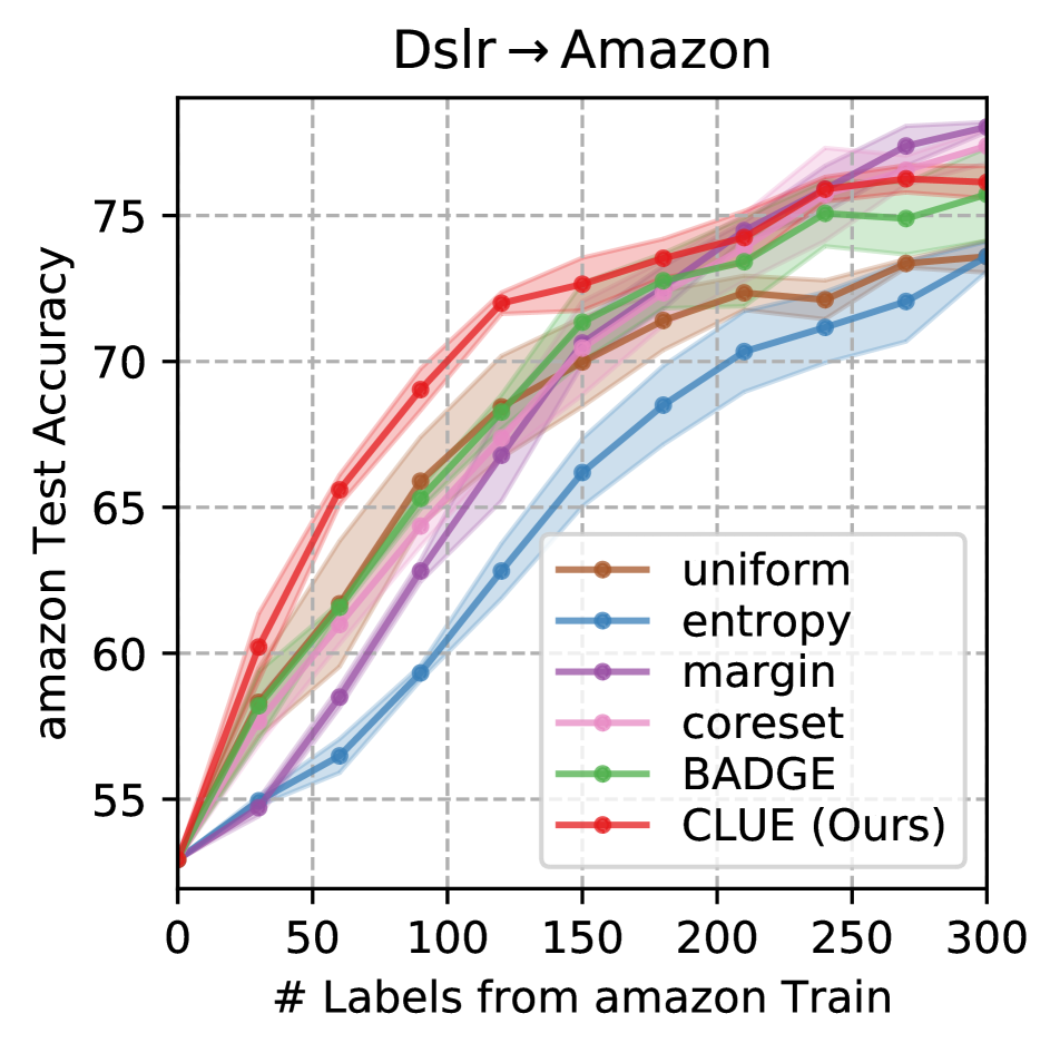
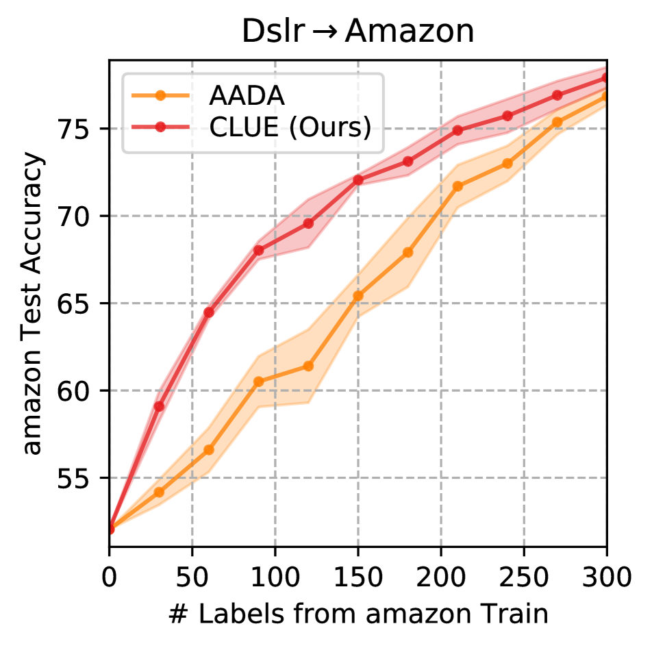
Metric. We compute model accuracy on the target test split versus the number of labels used from the target train split at each round. We run each experiment 3 times and report mean accuracies. For clarity, we report performance at 3 randomly chosen intermediate budgets in the main paper and include full plots (mean accuracies and 1 standard deviation over all rounds) in the supplementary.
4.2 Implementation details
DomainNet. We use a ResNet34 [20] CNN, and perform 10 rounds of Active DA with a randomly selected per-round budget instances (total of 5000 labels). On DomainNet, we use the ClipartSketch shift as a validation shift and use a small target validation set to select a softmax temperature of which we use for all other DomainNet shifts (details in supplementary). We include a sensitivity analysis over and in Sec. 4.5.
DIGITS. We match the experimental setting to Su et al. [47]: we use a modified LeNet architecture [21], and perform 30 rounds of Active DA with B10.
Office. We use a ResNet34 CNN and perform 10 rounds of Active DA with B30. On DIGITS and Office, we use the default value of . Across datasets, we use penultimate layer embeddings for CLUE and implement weighted K-means with . All models are first trained on the labeled source domain. When adapting via semi-supervised domain adaptation, we additionally employ unsupervised feature alignment to the target domain at round 0. For additional details see supplementary.
4.3 Baselines
We compare CLUE against several state-of-the art methods for Active DA and Active Learning.
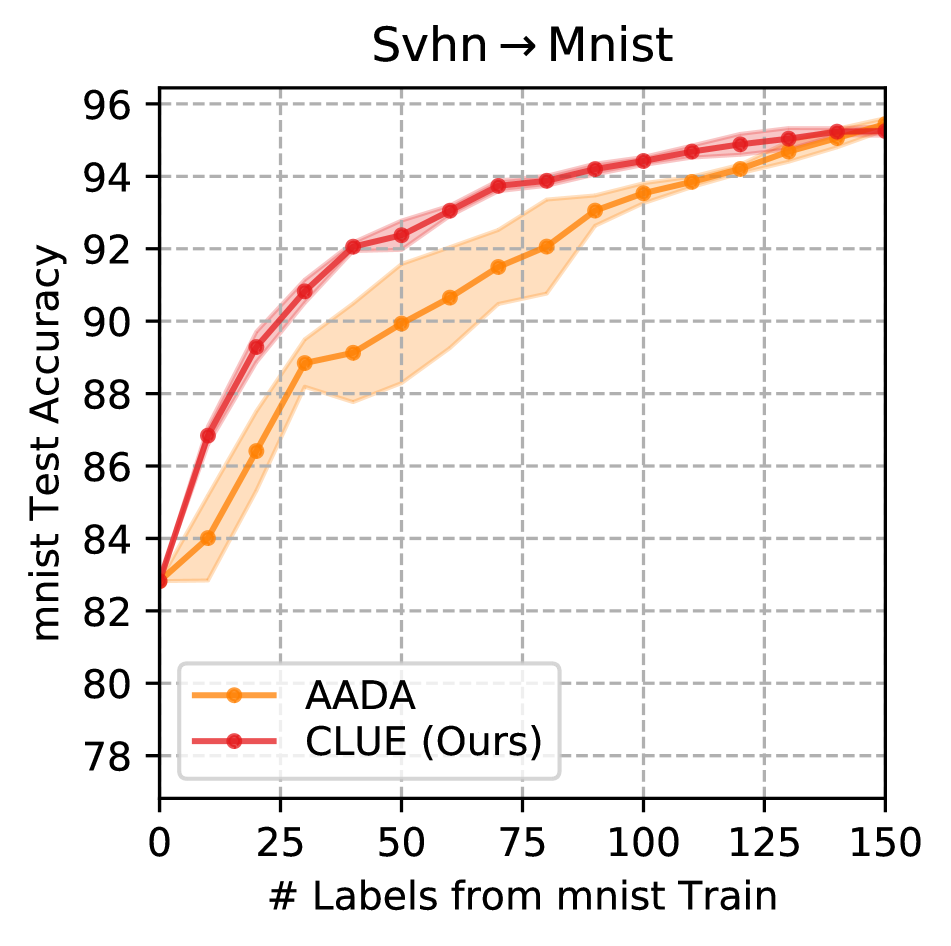
1) AADA: Active Adversarial Domain Adaptation [47] (AADA) is a state-of-the-art Active DA method which performs alternate rounds of active sampling and adversarial domain adaptation via DANN [14]. It samples points with high predictive entropy and high probability of belonging to the target domain as predicted by the domain discriminator.
Further, we also benchmark the performance of 4 diverse AL strategies from prior work in the Active DA setting.
2) entropy [52]: Selects instances for which the model has highest predictive entropy.
3) margin [37]: Selects instances for which the score difference between the model’s top-2 predictions is the smallest.
4) coreset [42]: Core-set formulates active sampling as a set-cover problem, and solves the K-Center [53] problem. We use the greedy version proposed in Sener et al. [42].
5) BADGE [2]: BADGE is a recently proposed state-of-the-art active learning strategy that constructs diverse batches by running KMeans++ [1] on “gradient embeddings” that incorporate model uncertainty and diversity.
Methods (2) and (3) are uncertainty based, (4) is diversity-based, and (1) and (5) are hybrid approaches.
| DA method | AL method | AL | (easy) | (moderate) | (hard) | (very hard) | AVG | ||||||||||
| Type | 1k | 2k | 5k | 1k | 2k | 5k | 1k | 2k | 5k | 1k | 2k | 5k | 1k | 2k | 5k | ||
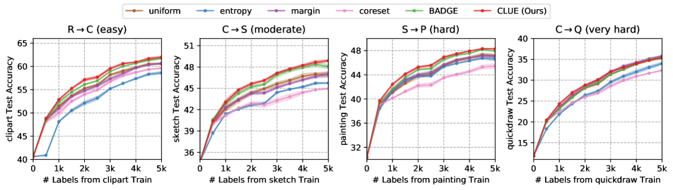
| ft from source | uniform | - | 51.5 | 55.3 | 60.6 | 42.1 | 44.4 | 47.0 | 41.1 | 43.8 | 47.2 | 23.3 | 28.1 | 35.3 | 39.5 | 42.9 | 47.5 |
| entropy [52] | U | 48.1 | 52.1 | 58.6 | 41.1 | 42.7 | 45.7 | 41.2 | 43.8 | 47.2 | 21.9 | 26.4 | 34.0 | 38.1 | 41.3 | 46.4 | |
| margin [37] | U | 51.0 | 54.8 | 60.7 | 42.3 | 44.3 | 47.0 | 41.4 | 44.0 | 47.1 | 23.6 | 28.4 | 35.8 | 39.6 | 42.9 | 47.7 | |
| coreset [42] | D | 50.0 | 54.0 | 59.6 | 41.2 | 42.8 | 44.9 | 40.1 | 42.2 | 45.4 | 22.4 | 26.0 | 32.4 | 38.4 | 41.3 | 45.6 | |
| BADGE [2] | H | 52.4 | 56.1 | 61.7 | 42.8 | 45.2 | 48.1 | 41.7 | 44.9 | 47.9 | 23.1 | 28.2 | 35.5 | 39.8 | 43.6 | 48.3 | |
| CLUE (Ours) | H | 52.9 | 57.1 | 62.0 | 43.3 | 45.8 | 48.6 | 42.4 | 45.3 | 48.3 | 24.3 | 28.8 | 35.5 | 40.7 | 44.3 | 48.6 | |
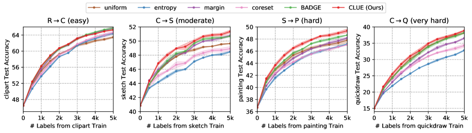
| MME [40] from source | uniform | - | 55.2 | 59.3 | 63.5 | 45.7 | 47.8 | 49.7 | 42.9 | 45.3 | 47.8 | 24.5 | 30.3 | 38.1 | 42.1 | 45.7 | 49.8 |
| entropy [52] | U | 53.8 | 58.6 | 64.4 | 44.2 | 45.7 | 48.5 | 41.6 | 43.9 | 47.2 | 21.9 | 25.7 | 32.8 | 40.4 | 43.5 | 48.2 | |
| margin [37] | U | 55.6 | 60.7 | 65.7 | 46.0 | 48.1 | 50.8 | 42.2 | 44.8 | 48.2 | 23.1 | 28.3 | 36.6 | 41.7 | 45.5 | 50.3 | |
| coreset [42] | D | 54.3 | 59.1 | 64.6 | 45.1 | 46.7 | 48.9 | 42.4 | 44.2 | 47.1 | 23.9 | 27.8 | 34.3 | 41.4 | 44.5 | 48.7 | |
| BADGE [2] | H | 56.2 | 60.6 | 65.7 | 45.8 | 48.2 | 50.7 | 43.1 | 45.7 | 48.7 | 24.3 | 29.6 | 38.3 | 42.4 | 46.0 | 50.9 | |
| CLUE (Ours) | H | 56.3 | 60.7 | 65.3 | 46.8 | 49.0 | 51.4 | 43.7 | 46.5 | 49.4 | 25.6 | 31.1 | 38.9 | 43.1 | 46.8 | 51.3 | |
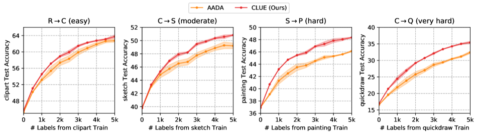
| DANN [13] | AADA [47] | H | 53.2 | 57.4 | 62.8 | 44.8 | 46.5 | 49.2 | 41.3 | 43.5 | 46.1 | 21.9 | 25.8 | 32.4 | 40.3 | 43.3 | 47.6 |
| from source | CLUE (Ours) | H | 54.6 | 58.9 | 63.8 | 45.3 | 47.9 | 50.8 | 43.2 | 45.5 | 48.3 | 24.4 | 29.2 | 35.4 | 41.9 | 45.4 | 49.6 |
| DA method | AL method | ||||||
| 30 | 60 | 150 | 30 | 60 | 150 | ||
| ft from source | uniform | 77.7 | 88.2 | 95.2 | 54.3 | 58.0 | 67.5 |
| entropy [52] | 65.8 | 75.6 | 92.9 | 51.2 | 52.4 | 59.1 | |
| margin [37] | 82.0 | 89.3 | 95.5 | 52.4 | 54.4 | 65.5 | |
| coreset [42] | 71.6 | 76.5 | 87.9 | 53.9 | 55.8 | 67.2 | |
| BADGE [2] | 78.7 | 88.2 | 95.2 | 55.8 | 59.2 | 71.0 | |
| CLUE (Ours) | 83.9 | 89.4 | 94.5 | 56.4 | 60.5 | 70.5 | |
| MME [40] from source | uniform | 85.5 | 91.2 | 95.0 | 58.3 | 61.7 | 70.0 |
| entropy [52] | 81.3 | 85.7 | 93.9 | 54.9 | 56.5 | 66.2 | |
| margin [37] | 88.4 | 91.5 | 96.6 | 54.7 | 58.5 | 70.6 | |
| coreset [42] | 85.8 | 89.1 | 94.6 | 57.7 | 61.0 | 70.5 | |
| BADGE [2] | 89.9 | 93.1 | 96.4 | 58.2 | 61.6 | 71.3 | |
| CLUE (Ours) | 91.1 | 93.9 | 96.2 | 60.2 | 65.6 | 72.7 | |
| DANN [13] | AADA [47] | 88.8 | 90.7 | 95.4 | 54.2 | 56.6 | 65.4 |
| from source | CLUE (Ours) | 90.9 | 93.1 | 95.3 | 59.1 | 64.5 | 72.1 |
4.4 Results
We evaluate all methods across three ways of learning in the presence of a domain shift with the acquired labels:
1) FT from source: Finetuning a model trained on the source domain with acquired target labels.
2) MME [40] from source: Minimax entropy [40] (MME) is a state-of-the-art semi-supervised DA method that starts from a source model and minimizes an adversarial entropy loss for unsupervised domain alignment in addition to finetuning on labeled source and target data.
Tables 13 and 2 demonstrate our results on DomainNet, DIGITS, and Office. We make the following observations:
Uncertainty and diversity sampling are less effective for Active DA, frequently underperforming even random sampling. Approaches solely based on uncertainty (e.g. margin [37]) work well on relatively easier shifts (RC with MME, SVHNMNIST), but overall we find uncertainty-based (margin, entropy), and diversity-based (coreset) approaches generalize poorly to challenging shifts (e.g. SP, CQ), frequently underperforming even random sampling! On the other hand, hybrid approaches (CLUE and BADGE) that combine uncertainty and diversity are versatile across shift difficulties.
CLUE outperforms prior AL methods in the Active DA setting. Across learning strategies, shifts, benchmarks, and most rounds, CLUE consistently performs best. Averaged over 4 DomainNet shifts, CLUE outperforms margin-based uncertainty sampling and coreset-based diversity sampling at by 1.4% and 3% when finetuning, and 1.3% and 2.3% when adapting via MME (Tab. 13). Similarly, CLUE outperforms the next best-performing method (BADGE) by 0.7% at when finetuning and 0.8% with MME (4 shift average). While BADGE [2] is also a hybrid AL method that combines uncertainty and diversity sampling, it does so by clustering in a high-dimensional “gradient-embedding” space (176k dimensions on CS with a ResNet34, versus 512-dimensional embeddings used by CLUE, details in Tab. 3), in which distance-based diversity measures may be less meaningful due to the curse of dimensionality. We note here that DomainNet is a complex benchmark with 345 categories and significant label noise, which often leads to relatively small absolute margins of improvement; however, our results demonstrate CLUE’s versatility in generalizing across diverse shifts without shift-specific tuning.
On DIGITS and Office, CLUE’s gains are even more significant (Tab. 2). For instance at on SVHNMNIST, CLUE improves upon margin, coreset, and BADGE when finetuning by 1.9%, 12.3%, and 5.2%, and 4%, 2.5% and 0.6% on DSLRAmazon.

Additional unsupervised adaptation helps in the Active DA setting. Across AL methods, we observe adaptation with MME to consistently outperform finetuning (e.g. by 2.4-2.7% accuracy on DomainNet).
CLUE significantly outperforms the state-of-the art Active DA method AADA. AADA [47] acquires labels by using a domain classifier learned via DANN [13]. Thus, it is undefined in the FT and MME settings. For an apples-to-apples comparison, we report performance of CLUE +DANN in the last 2 rows of Tabs. 13 and 2. As seen, CLUE +DANN consistently outperforms AADA, the state-of-the art Active DA method, e.g. by 0.4%-2% on DomainNet. Further, we find the performance gap between our method and AADA [47] increases with increasing shift difficulty, as predictive uncertainty becomes increasingly unreliable (3.4% gain at on the very hard CQ shift). We observe similar improvements over AADA on the DIGITS and Office (Tab. 2) benchmarks, e.g. 2.4% and 7.9% at . Further, our best performing CLUE + MME strategy improves the gains still further to as much as 3.5% at on DomainNet and 9% at on Office!
As discussed in Sec. 3, the optimal label acquisition criterion may vary across shifts and stages of training as the model’s uncertainty estimates and feature space evolve, and it is challenging for a single approach to work well consistently. Despite this, CLUE effectively trades-off uncertainty and diversity to generalize reliably across shifts.
4.5 Analyzing and Ablating CLUE
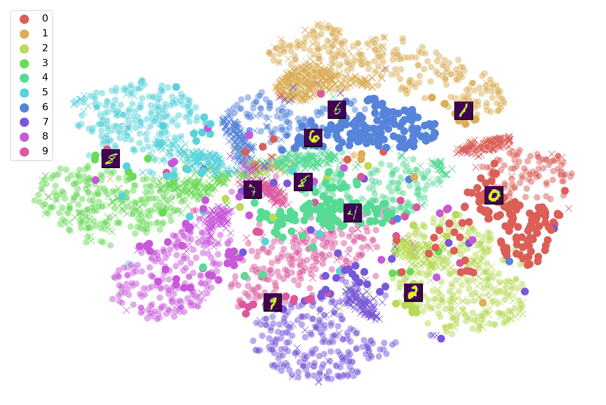
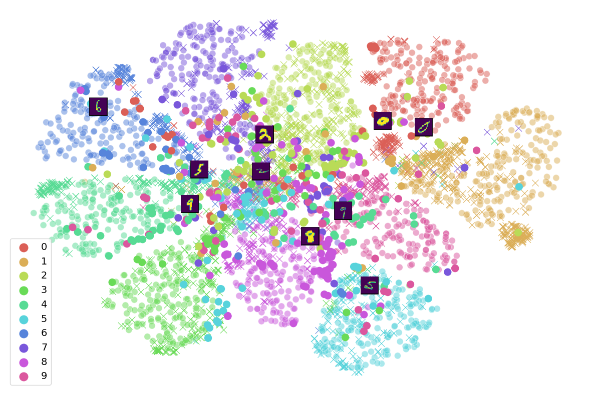
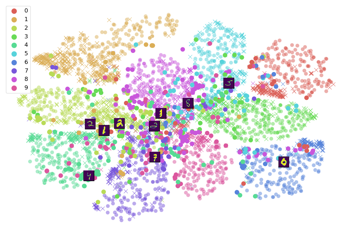
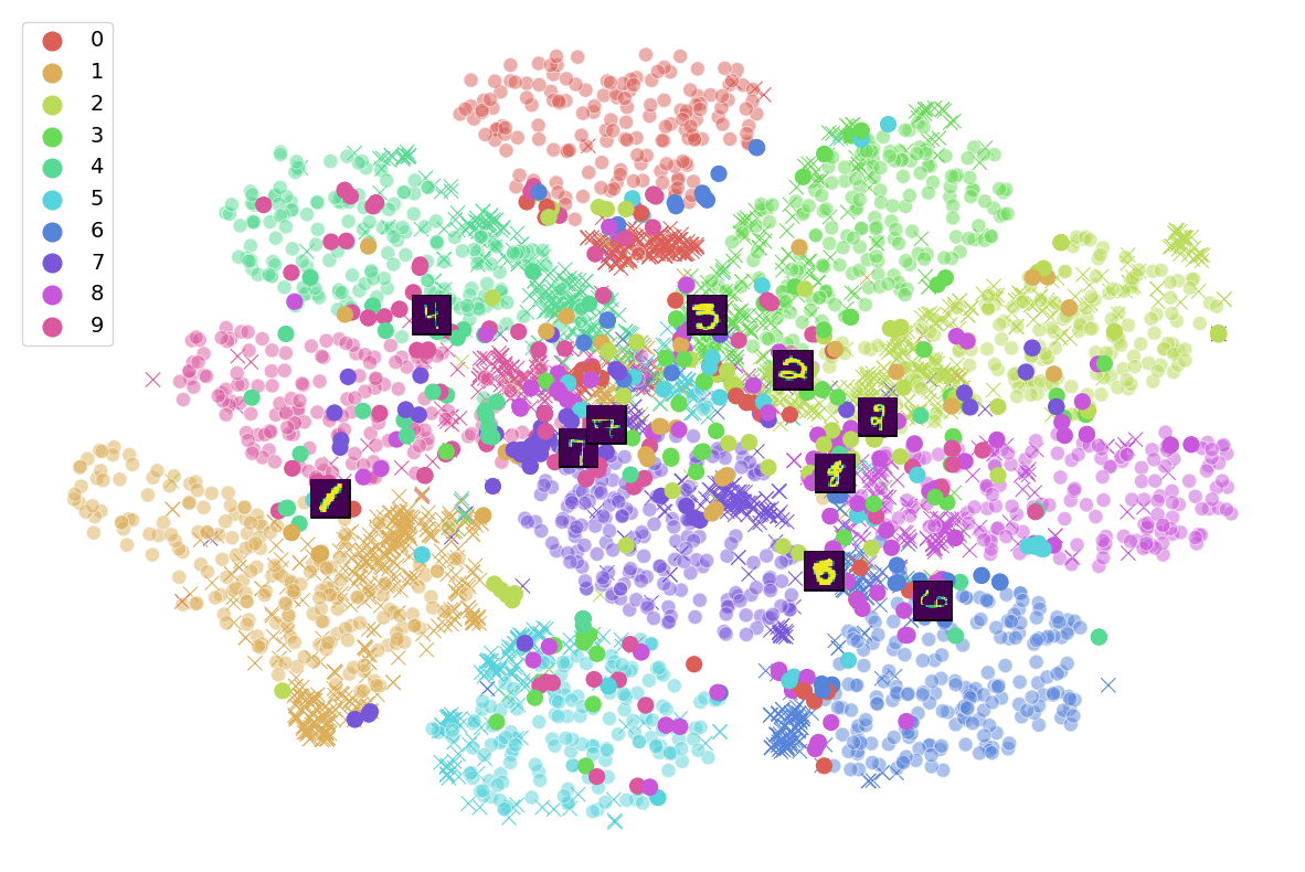
Visualizing CLUE via t-SNE. We provide an illustrative comparison of sampling strategies using t-SNE [30]. Fig. 3 shows an initial feature landscape together with points selected by entropy-based uncertainty sampling, diversity-based coreset sampling, and CLUE at Round 0 on the SVHNMNIST shift. We find that entropy [52] (left) samples uncertain but redundant points, coreset [42] samples diverse but not necessarily uncertain points, while our method, CLUE, samples both diverse and uncertain points. In the supplementary, we include visualizations over several rounds and find that CLUE consistently selects diverse target instances from dense, uncertain regions of the feature space.
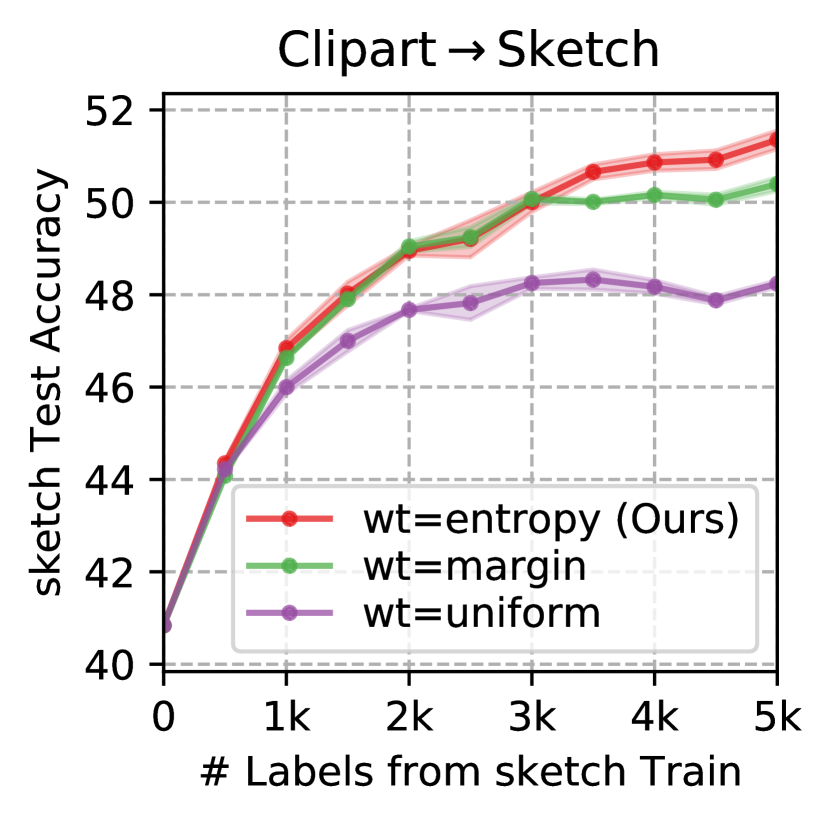
Varying uncertainty measure in CLUE. In Fig. 4(a), we consider alternative uncertainty measures for CLUE on the CS shift. We show that our proposed use of sample entropy significantly outperforms a uniform sample weight and narrowly outperforms an alternative uncertainty measure - sample margin score (difference between scores for top-2 most likely classes). This illustrates the importance of using uncertainty-weighting to bias CLUE towards informative samples. We also experimented (not shown) with last-layer embeddings (instead of penultimate) for CLUE, and observed near-identical performance across multiple shifts, suggesting that CLUE is not sensitive to this choice.
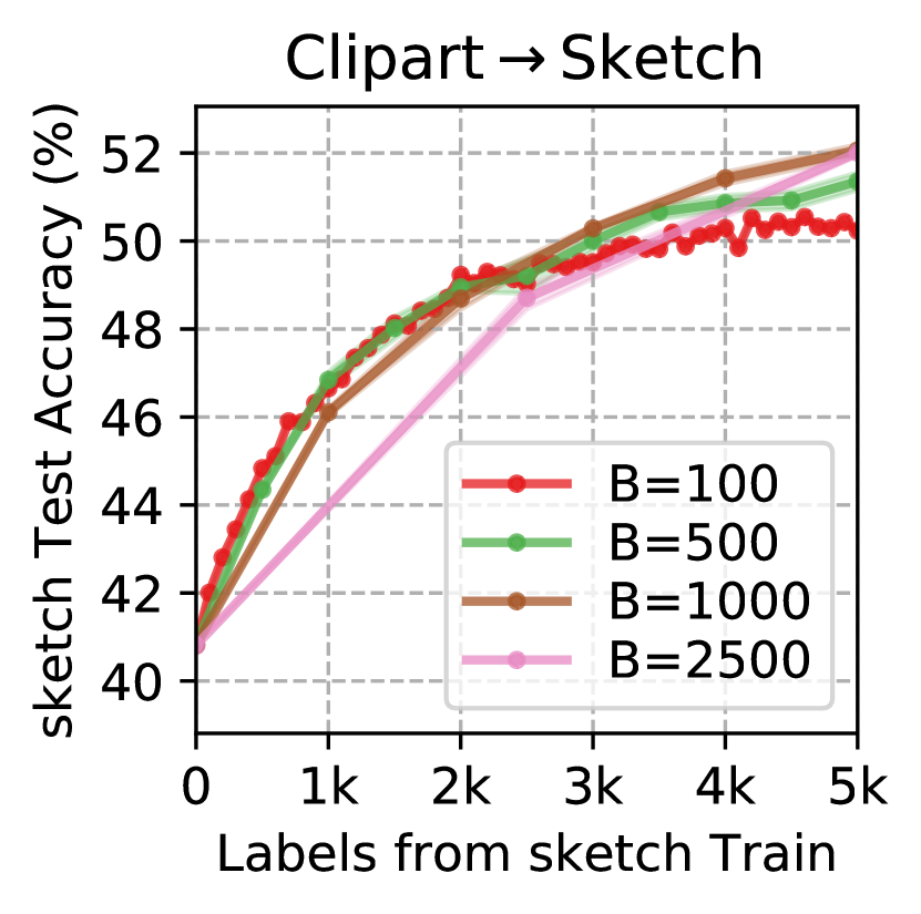
Sensitivity to parameters. In Fig. 4 we measure CLUE’s sensitivity to two parameters: the softmax temperature hyperparameter T and experimental parameter budget B.
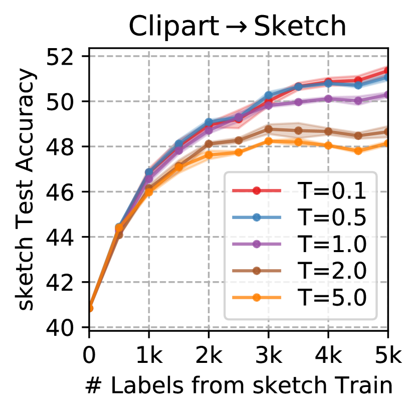
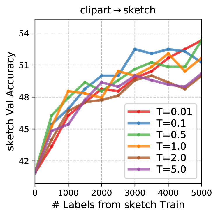
i) Sensitivity to softmax temperature T. Recall from Sec. 3 that by tuning the softmax temperature in CLUE, we can vary the trade-off between uncertainty and diversity. In Fig. 4(b) we run a sweep over temperature values used for CLUE on CS . As seen, lower values of temperature (which emphasizes the role of uncertainty) improve performance, particularly at later rounds when uncertainty estimates are more reliable. We note that is an optional hyperparameter that may be tuned if a small target validation set is available, but CLUE obtains strong state-of-the art results across across DIGITS, Office, and DomainNet even with the default value of T=1.0. On DomainNet, we further improve performance by selecting via grid search on a single CS shift and find that it generalizes to other DomainNet shifts.
ii) Sensitivity to budget B. We now vary the per-round budget (and consequently the total number of active adaptation rounds) and report performance on the ClipartSketch shift. As seen in Fig. 4(c), CLUE performs well across budget values of 100, 500, 1k and 2.5k. We also observe consistent performance with a different budget () on the SVHNMNIST shift (details in supplementary).
Time complexity. Table 3 shows the average case complexity and AL querying time-per-round on SVHNMNIST and CS. CLUE and BADGE, which achieve the best accuracy, are slower to run due to a (CPU) clustering step. CLUE can be optimized further via GPU acceleration, using last-(instead of penultimate) layer embeddings, or pre-filtering data before clustering.
|
|
|
|||||||
| fwd + cluster | CLUE (Ours) | (60s, 16.2m) | |||||||
| BADGE [2] | (103s, 16.3m) | ||||||||
| coreset [42] | (52s, 2.8m) | ||||||||
| fwd + rank | AADA [47] | (3.7s, 139s) | |||||||
| entropy [52] | (3.5s, 45s) | ||||||||
| margin [37] | (3.2s, 45s) |
4.6 CLUE across learning strategies
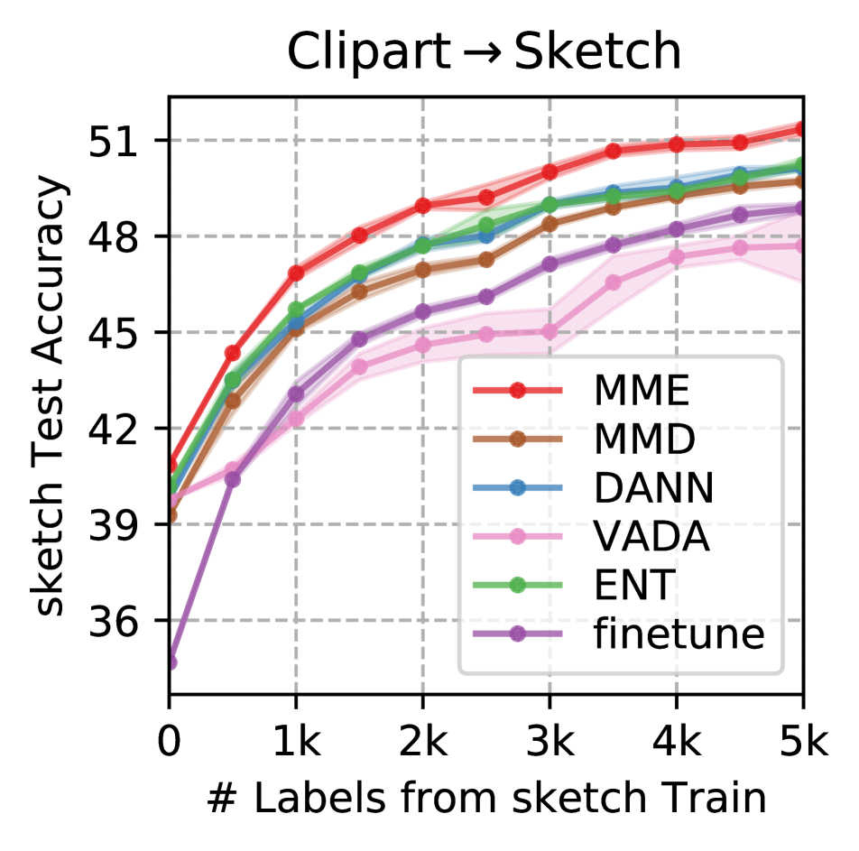
CLUE with different DA strategies. We now study CLUE’s compatibility with a few additional domain adaptation strategies from the literature. In addition to the finetuning, DANN [13] and MME [40] already studied in Sec. 4.4, we fix our sampling strategy to CLUE and vary the learning strategy to: i) MMD [29], a discrepancy-statistic based DA method, and ii) VADA [44], a domain-classifier based method that uses virtual adversarial training. iii) ENT [17]: A variant of the MME method using standard rather than adversarial entropy minimization. Initial performance varies across methods since we employ unsupervised DA at Round 0.
In Fig. 4(d), we observe that domain alignment with MME significantly outperforms all alternative methods. With all DA methods except VADA, we observe improvements over finetuning; however, MME clearly performs best. The improvements over DANN and VADA are consistent with Saito et al. [40], who find that domain-classifier based methods are less effective when some target labels are available.
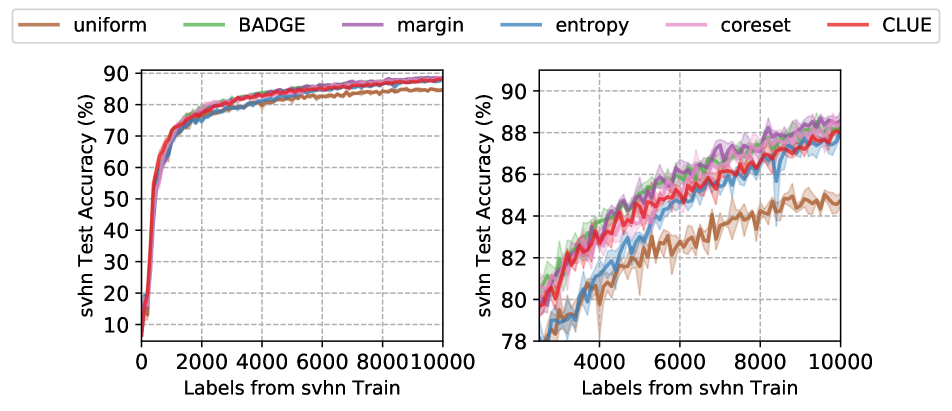
How well does CLUE learn from scratch? While CLUE is designed for active learning under a domain shift, for completeness we also evaluate its performance against prior work when learning from “scratch” as is conventional in AL. We find that it outperforms prior work when finetuning using ImageNet [38] initialization on CS, and performs on par with competing methods when finetuning from scratch on SVHN [31] (details in supplementary).
5 Conclusion
We address active domain adaptation, where the goal is to select target instances for labeling so as to generalize a trained source model to a new target domain. We show how existing active learning strategies based solely on uncertainty or diversity sampling are not effective for Active DA. We present CLUE, a novel label acquisition strategy for active sampling under a domain shift, that performs uncertainty-weighted clustering to select diverse, informative target instances for labeling from dense regions of the feature space. We demonstrate CLUE’s effectiveness over competing active learning and Active DA methods across learning settings and domain shifts, and comprehensively analyze its behavior.
Acknowledgements. This work was supported by the DARPA LwLL program. We would like to thank Devi Parikh for guidance, and Prithvijit Chattopadhyay, Cornelia Köhler, and Shruti Venkatram for feedback on the draft.
References
- [1] David Arthur and Sergei Vassilvitskii. k-means++: The advantages of careful seeding. Technical report, Stanford, 2006.
- [2] Jordan T Ash, Chicheng Zhang, Akshay Krishnamurthy, John Langford, and Alekh Agarwal. Deep batch active learning by diverse, uncertain gradient lower bounds. In International Conference on Learning Representations, 2020.
- [3] Yoram Baram, Ran El Yaniv, and Kobi Luz. Online choice of active learning algorithms. Journal of Machine Learning Research, 5(Mar):255–291, 2004.
- [4] Klaus Brinker. Incorporating diversity in active learning with support vector machines. In Proceedings of the 20th international conference on machine learning (ICML-03), pages 59–66, 2003.
- [5] Rita Chattopadhyay, Wei Fan, Ian Davidson, Sethuraman Panchanathan, and Jieping Ye. Joint transfer and batch-mode active learning. In International Conference on Machine Learning, pages 253–261, 2013.
- [6] Wei-Yu Chen, Yen-Cheng Liu, Zsolt Kira, Yu-Chiang Wang, and Jia-Bin Huang. A closer look at few-shot classification. In International Conference on Learning Representations, 2019.
- [7] David Cohn, Les Atlas, and Richard Ladner. Improving generalization with active learning. Machine learning, 15(2):201–221, 1994.
- [8] A David. Vassilvitskii s.: K-means++: The advantages of careful seeding. In 18th annual ACM-SIAM symposium on Discrete algorithms (SODA), New Orleans, Louisiana, pages 1027–1035, 2007.
- [9] Jeff Donahue, Judy Hoffman, Erik Rodner, Kate Saenko, and Trevor Darrell. Semi-supervised domain adaptation with instance constraints. In Proceedings of the IEEE conference on computer vision and pattern recognition, pages 668–675, 2013.
- [10] Melanie Ducoffe and Frederic Precioso. Adversarial active learning for deep networks: a margin based approach. arXiv preprint arXiv:1802.09841, 2018.
- [11] Charles Elkan. Using the triangle inequality to accelerate k-means. In Proceedings of the 20th international conference on machine learning (ICML-03), pages 147–153, 2003.
- [12] Yarin Gal, Riashat Islam, and Zoubin Ghahramani. Deep bayesian active learning with image data. In Proceedings of the 34th International Conference on Machine Learning-Volume 70, pages 1183–1192. JMLR. org, 2017.
- [13] Yaroslav Ganin and Victor Lempitsky. Unsupervised domain adaptation by backpropagation. In International Conference on Machine Learning, pages 1180–1189, 2015.
- [14] Yaroslav Ganin, Evgeniya Ustinova, Hana Ajakan, Pascal Germain, Hugo Larochelle, François Laviolette, Mario Marchand, and Victor Lempitsky. Domain-adversarial training of neural networks. The Journal of Machine Learning Research, 17(1):2096–2030, 2016.
- [15] Yonatan Geifman and Ran El-Yaniv. Deep active learning over the long tail. arXiv preprint arXiv:1711.00941, 2017.
- [16] Daniel Gissin and Shai Shalev-Shwartz. Discriminative active learning. arXiv preprint arXiv:1907.06347, 2019.
- [17] Yves Grandvalet, Yoshua Bengio, et al. Semi-supervised learning by entropy minimization. In CAP, pages 281–296, 2005.
- [18] Greg Hamerly and Charles Elkan. Alternatives to the k-means algorithm that find better clusterings. In Proceedings of the eleventh international conference on Information and knowledge management, pages 600–607, 2002.
- [19] John A Hartigan and Manchek A Wong. Algorithm as 136: A k-means clustering algorithm. Journal of the Royal Statistical Society. Series C (Applied Statistics), 28(1):100–108, 1979.
- [20] Kaiming He, Xiangyu Zhang, Shaoqing Ren, and Jian Sun. Deep residual learning for image recognition. In Proceedings of the IEEE conference on computer vision and pattern recognition, pages 770–778, 2016.
- [21] Judy Hoffman, Eric Tzeng, Taesung Park, Jun-Yan Zhu, Phillip Isola, Kate Saenko, Alexei Efros, and Trevor Darrell. Cycada: Cycle-consistent adversarial domain adaptation. In International Conference on Machine Learning, pages 1989–1998, 2018.
- [22] Wei-Ning Hsu and Hsuan-Tien Lin. Active learning by learning. In Twenty-Ninth AAAI conference on artificial intelligence, 2015.
- [23] Joshua Zhexue Huang, Michael K Ng, Hongqiang Rong, and Zichen Li. Automated variable weighting in k-means type clustering. IEEE transactions on pattern analysis and machine intelligence, 27(5):657–668, 2005.
- [24] Diederik P Kingma and Jimmy Ba. Adam: A method for stochastic optimization. arXiv preprint arXiv:1412.6980, 2014.
- [25] Andreas Kirsch, Joost van Amersfoort, and Yarin Gal. Batchbald: Efficient and diverse batch acquisition for deep bayesian active learning. In Advances in Neural Information Processing Systems, pages 7024–7035, 2019.
- [26] Hans-Peter Kriegel, Erich Schubert, and Arthur Zimek. The (black) art of runtime evaluation: Are we comparing algorithms or implementations? Knowledge and Information Systems, 52(2):341–378, 2017.
- [27] Yann LeCun, Léon Bottou, Yoshua Bengio, and Patrick Haffner. Gradient-based learning applied to document recognition. Proceedings of the IEEE, 86(11):2278–2324, 1998.
- [28] Mingsheng Long, Yue Cao, Jianmin Wang, and Michael Jordan. Learning transferable features with deep adaptation networks. In International Conference on Machine Learning, pages 97–105, 2015.
- [29] Mingsheng Long, Jianmin Wang, Guiguang Ding, Jiaguang Sun, and Philip S Yu. Transfer feature learning with joint distribution adaptation. In Proceedings of the IEEE international conference on computer vision, pages 2200–2207, 2013.
- [30] Laurens van der Maaten and Geoffrey Hinton. Visualizing data using t-sne. Journal of machine learning research, 9(Nov):2579–2605, 2008.
- [31] Yuval Netzer, Tao Wang, Adam Coates, Alessandro Bissacco, Bo Wu, and Andrew Y Ng. Reading digits in natural images with unsupervised feature learning. In Neural Information Processing Systems (NeurIPS), 2011.
- [32] Adam Paszke, Sam Gross, Francisco Massa, Adam Lerer, James Bradbury, Gregory Chanan, Trevor Killeen, Zeming Lin, Natalia Gimelshein, Luca Antiga, et al. Pytorch: An imperative style, high-performance deep learning library. In Advances in Neural Information Processing Systems, pages 8024–8035, 2019.
- [33] Fabian Pedregosa, Gaël Varoquaux, Alexandre Gramfort, Vincent Michel, Bertrand Thirion, Olivier Grisel, Mathieu Blondel, Peter Prettenhofer, Ron Weiss, Vincent Dubourg, et al. Scikit-learn: Machine learning in python. the Journal of machine Learning research, 12:2825–2830, 2011.
- [34] Xingchao Peng, Qinxun Bai, Xide Xia, Zijun Huang, Kate Saenko, and Bo Wang. Moment matching for multi-source domain adaptation. In Proceedings of the IEEE International Conference on Computer Vision, pages 1406–1415, 2019.
- [35] George R Price. Extension of covariance selection mathematics. Annals of human genetics, 35(4):485–490, 1972.
- [36] Piyush Rai, Avishek Saha, Hal Daumé III, and Suresh Venkatasubramanian. Domain adaptation meets active learning. In Proceedings of the NAACL HLT 2010 Workshop on Active Learning for Natural Language Processing, pages 27–32. Association for Computational Linguistics, 2010.
- [37] Dan Roth and Kevin Small. Margin-based active learning for structured output spaces. In European Conference on Machine Learning, pages 413–424. Springer, 2006.
- [38] Olga Russakovsky, Jia Deng, Hao Su, Jonathan Krause, Sanjeev Satheesh, Sean Ma, Zhiheng Huang, Andrej Karpathy, Aditya Khosla, Michael Bernstein, et al. Imagenet large scale visual recognition challenge. International journal of computer vision, 115(3):211–252, 2015.
- [39] Kate Saenko, Brian Kulis, Mario Fritz, and Trevor Darrell. Adapting visual category models to new domains. In European conference on computer vision, pages 213–226. Springer, 2010.
- [40] Kuniaki Saito, Donghyun Kim, Stan Sclaroff, Trevor Darrell, and Kate Saenko. Semi-supervised domain adaptation via minimax entropy. In Proceedings of the IEEE International Conference on Computer Vision, pages 8050–8058, 2019.
- [41] Greg Schohn and David Cohn. Less is more: Active learning with support vector machines. In ICML, volume 2, page 6. Citeseer, 2000.
- [42] Ozan Sener and Silvio Savarese. Active learning for convolutional neural networks: A core-set approach. In International Conference on Learning Representations, 2018.
- [43] Burr Settles. Active learning literature survey. Technical report, University of Wisconsin-Madison Department of Computer Sciences, 2009.
- [44] Rui Shu, Hung H Bui, Hirokazu Narui, and Stefano Ermon. A dirt-t approach to unsupervised domain adaptation. In Proc. 6th International Conference on Learning Representations, 2018.
- [45] Samarth Sinha, Sayna Ebrahimi, and Trevor Darrell. Variational adversarial active learning. In Proceedings of the IEEE International Conference on Computer Vision, pages 5972–5981, 2019.
- [46] Jasper Snoek, Yaniv Ovadia, Emily Fertig, Balaji Lakshminarayanan, Sebastian Nowozin, D Sculley, Joshua Dillon, Jie Ren, and Zachary Nado. Can you trust your model’s uncertainty? evaluating predictive uncertainty under dataset shift. In Advances in Neural Information Processing Systems, pages 13969–13980, 2019.
- [47] Jong-Chyi Su, Yi-Hsuan Tsai, Kihyuk Sohn, Buyu Liu, Subhransu Maji, and Manmohan Chandraker. Active adversarial domain adaptation. In The IEEE Winter Conference on Applications of Computer Vision, pages 739–748, 2020.
- [48] Simon Tong and Daphne Koller. Support vector machine active learning with applications to text classification. Journal of machine learning research, 2(Nov):45–66, 2001.
- [49] Antonio Torralba and Alexei A Efros. Unbiased look at dataset bias. In Proceedings of the IEEE Conference on Computer Vision and Pattern Recognition, pages 1521–1528. IEEE, 2011.
- [50] Eric Tzeng, Judy Hoffman, Kate Saenko, and Trevor Darrell. Adversarial discriminative domain adaptation. In Proceedings of the IEEE Conference on Computer Vision and Pattern Recognition, pages 7167–7176, 2017.
- [51] Eric Tzeng, Judy Hoffman, Ning Zhang, Kate Saenko, and Trevor Darrell. Deep domain confusion: Maximizing for domain invariance. arXiv preprint arXiv:1412.3474, 2014.
- [52] Dan Wang and Yi Shang. A new active labeling method for deep learning. In 2014 International joint conference on neural networks (IJCNN), pages 112–119. IEEE, 2014.
- [53] Gert W Wolf. Facility location: concepts, models, algorithms and case studies. series: Contributions to management science: edited by zanjirani farahani, reza and hekmatfar, masoud, heidelberg, germany, physica-verlag, 2009, 2011.
- [54] Ting Yao, Yingwei Pan, Chong-Wah Ngo, Houqiang Li, and Tao Mei. Semi-supervised domain adaptation with subspace learning for visual recognition. In Proceedings of the IEEE conference on Computer Vision and Pattern Recognition, pages 2142–2150, 2015.
- [55] Yuli Zhang, Huaiyu Wu, and Lei Cheng. Some new deformation formulas about variance and covariance. In 2012 Proceedings of International Conference on Modelling, Identification and Control, pages 987–992. IEEE, 2012.
- [56] Fedor Zhdanov. Diverse mini-batch active learning. arXiv preprint arXiv:1901.05954, 2019.
6 Appendix
6.1 Performance of CLUE on Standard AL
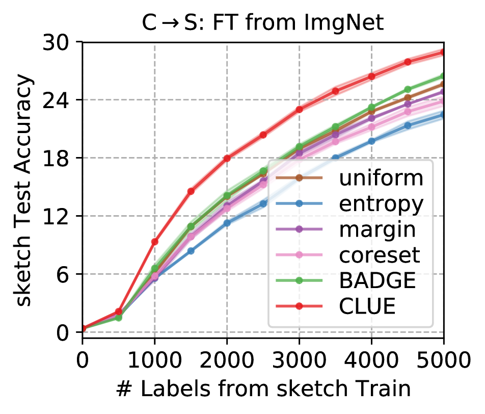
While CLUE is designed as an Active DA strategy, we nevertheless study its suitability for traditional active learning in which models are typically trained from “scratch”. We benchmark its performance against competing methods in two settings: Finetuning from an ImageNet [38] initialization on the ClipartSketch shift from DomainNet, following the same experimental protocol we use for Active DA (but set softmax temperature T as uncertainty is less reliable when learning from scratch), and the standard SVHN benchmark used for active learning [2]. For AL on SVHN, we match the setting in Ash et al. [2], initializing a ResNet18 [20] CNN with random weights and perform 100 rounds of active learning with per-round budget of 100. As summarized in Figure 6(a), on DomainNet CLUE significantly outpeforms prior work. On SVHN (Fig 6(b)), CLUE is on-par with state-of-the-art AL methods, and statistically significantly better than uniform sampling over most rounds.
6.2 Analyzing CLUE: When do gains saturate?
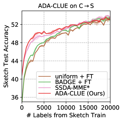
Due to the computational expense of running active domain adaptation on multiple shifts with a large CNN (ResNet34 [20]) on a large dataset (DomainNet [34]), in the main paper we restrict ourselves to 10 rounds with a per-round budget of 500. As a check on when performance gains saturate, we benchmark performance of CLUE + MME [40] on ClipartSketch for 40 rounds with per-round budget of 500 ( labels in total), against a few representative baselines: BADGE [2]+FT (state-of-the-art AL method with finetuning), uniform+MME [40] (uniform sampling with state-of-the-art semi-supervised DA method), and uniform + FT (uniform sampling with finetuning). Results are presented in Fig. 5. As seen, CLUE’s strongest performance improvements are seen in the initial stages of training, where it significantly outperforms competing methods. Performance then begins to saturate roughly around the 15k labels mark, and performance differences across methods narrow.
6.3 Comparing CLUE and BADGE
Both CLUE and BADGE are hybrid label acqusition strategies that combine uncertainty and diversity sampling. We now elaborate upon the differences between the two:
Conceptual comparison. CLUE and BADGE conceptually differ in 3 key ways: i) Feature space. BADGE: Operates in “gradient embedding” space computed as an outer product of penultimate-layer instance embeddings and model output scores. CLUE: Operates on penultimate-layer embeddings scaled by model uncertainty. ii) Uncertainty measure. BADGE: Uses gradient wrt model’s top-1 prediction. CLUE: Uses predictive entropy. iii) Diversity measure. BADGE: Runs KMeans++ in gradient embedding space. CLUE: Runs uncertainty-weighted K-Means on instance embeddings and selects nearest neighbors to centroids.
These design choices influence both BADGE’s effectiveness and efficiency. For dim. penultimate-layer embeddings and dim. (for classes) output scores, each gradient embedding has -dims – on DomainNet, this is -dims with a ResNet34 and 1.4 million dims with AlexNet. In addition to being expensive to compute, KMeans++ in such high dimensional spaces is less effective as distance measures becomes less reliable. In comparison, CLUE operates in a significantly lower-dimensional feature space (512/4096 for ResNet34/AlexNet). We believe these differences lead to CLUE being more computationally efficient (Tab. 3 in main paper) and effective on average than BADGE (Tab. 1-2 in main paper), especially on hard shifts (e.g. SP, CQ in Tab. 1 of main paper).
| AL method | ||||||
| 30 | 60 | 150 | 30 | 60 | 150 | |
| BADGE | 89.9 | 93.1 | 96.4 | 58.2 | 61.6 | 71.3 |
| CLUE | 91.1 | 93.9 | 96.2 | 60.2 | 65.6 | 72.7 |
Empirical comparison. On DomainNet, CLUE achieves small but consistent gains over BADGE (Tab. 1 in main paper) – with MME, across 4 diverse shifts 10 rounds = settings, and accounting for error bars, CLUE does as well or better than BADGE on 38/40 (better on 24/40). On other benchmarks, we sometimes observe large gains on other benchmarks (+5.2% on DIGITS at B=30, Tab. 2). However, at later rounds on SVHNMNIST and DSLRAmazon, BADGE and CLUE perform similarly. With MME, and after including error bars, CLUE matches or outperforms BADGE on 24/30 (DIGITS) and 10/10 (Office) settings (Tab. 4 shows 3 budgets), with BADGE doing slightly better from rounds 20-24 on DIGITS. We conjecture this is because gradient embedding dimensionality on DIGITS for 10-way classification is low, which leads to BADGE being as effective.
6.4 Dataset details
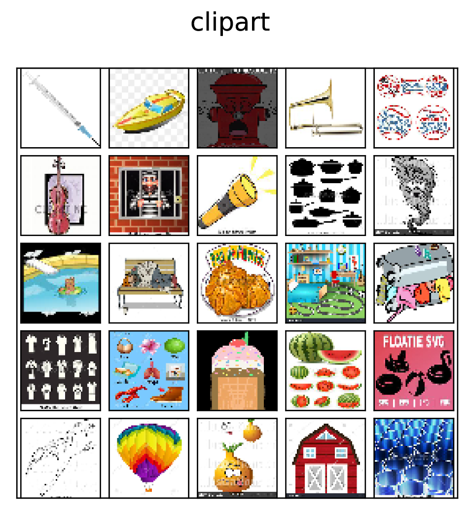
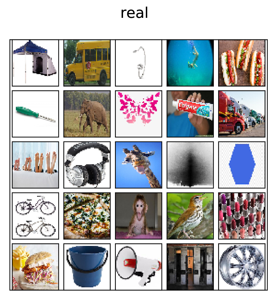
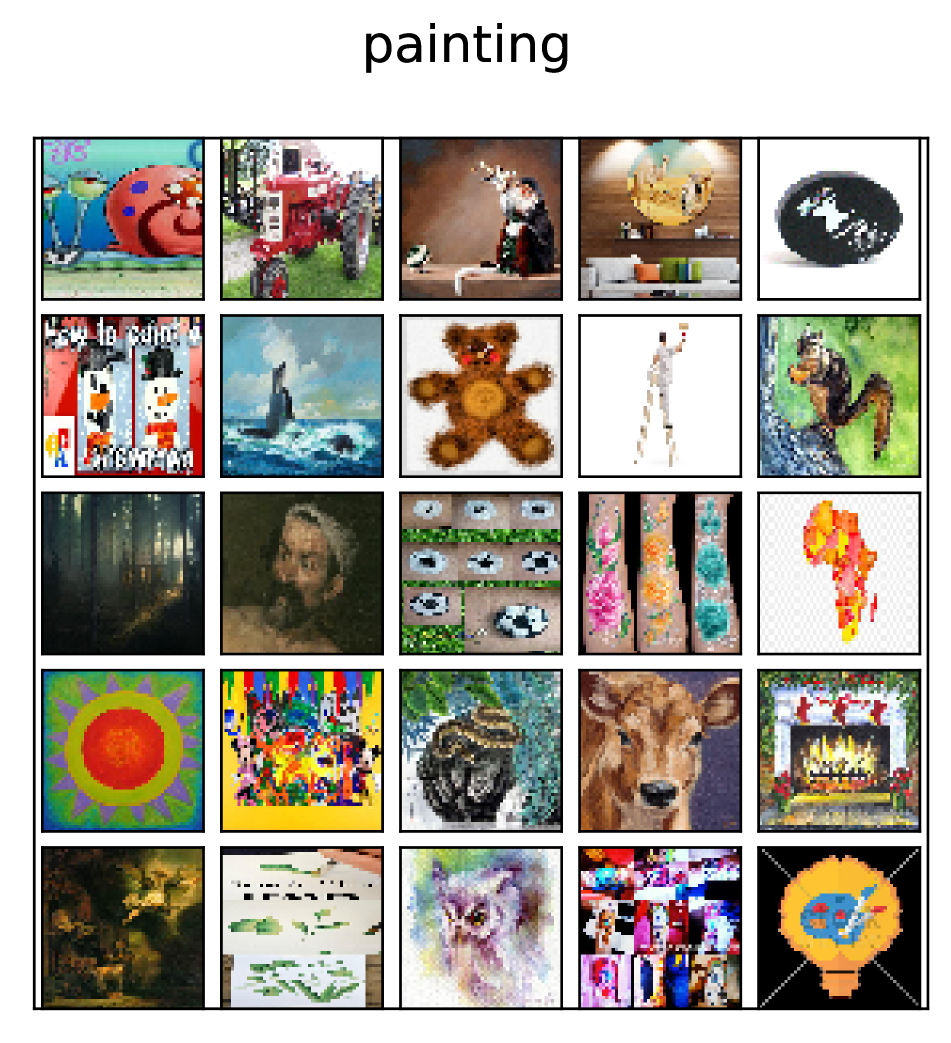
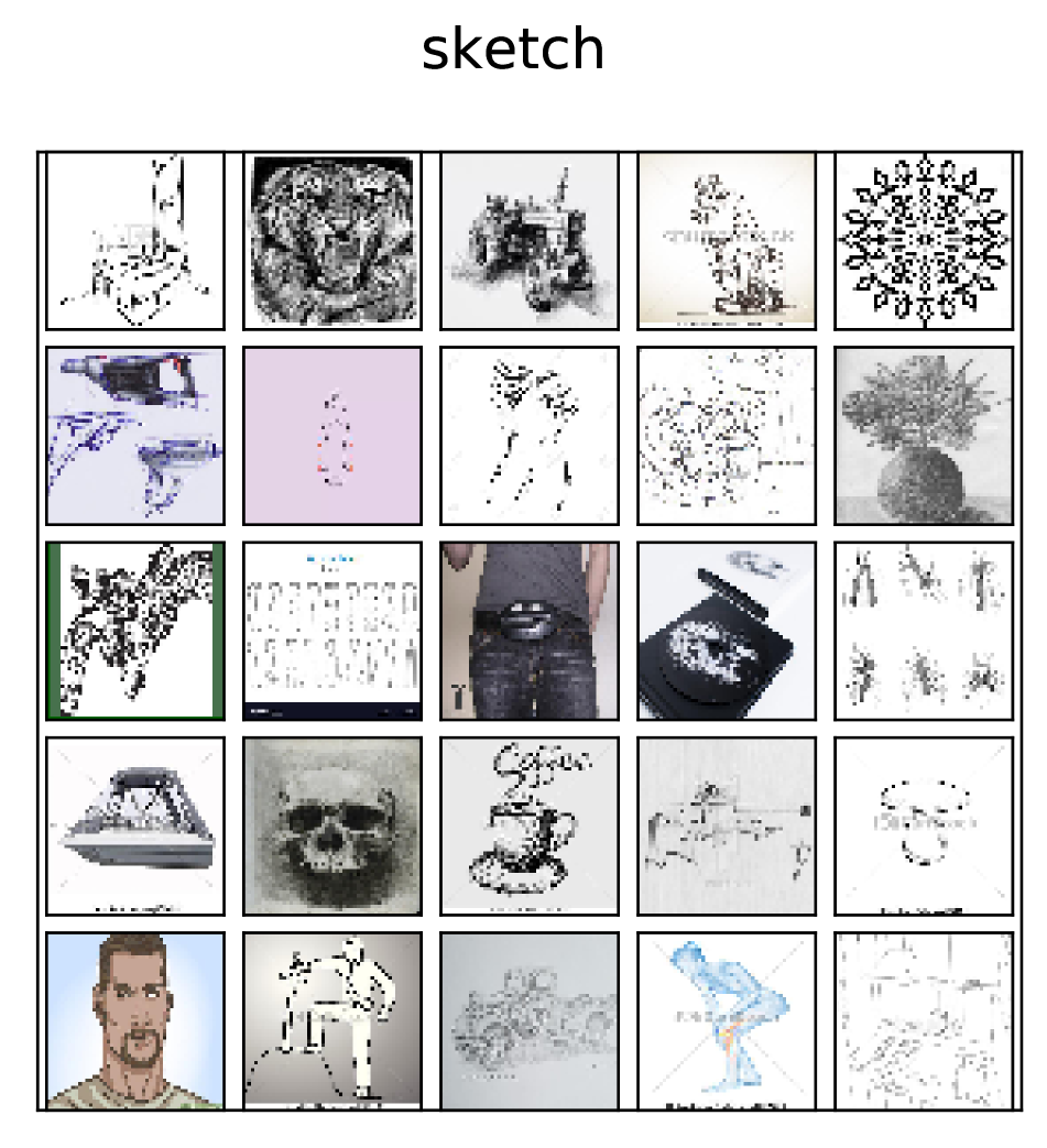
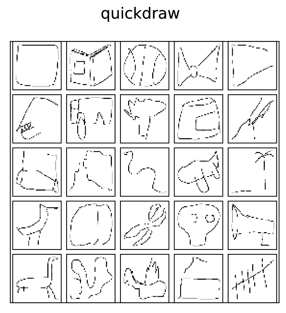
DomainNet. For our primary experiments, we use the DomainNet [34] dataset that consists of 0.6 million images spanning 6 domains, available at http://ai.bu.edu/M3SDA/. For our experiments, we use 4 shifts from 5 domains: Real, Clipart, Sketch, Painting, and Quickdraw. Table 5 summarizes the train/test statistics of each of these domains, while Fig. 8 provides representative examples from each. As models use ImageNet initialization, we avoid using Real as a target domain.
| Real | Clipart | Painting | Sketch | Quickdraw | |
| Train | 120906 | 33525 | 48212 | 50416 | 120750 |
| Test | 52041 | 14604 | 20916 | 21850 | 51750 |
6.5 Code and Implementation Details
We use PyTorch [32] for all our experiments. Most experiments were run on an NVIDIA TitanX GPU.
CLUE. We use the weighted K-Means implementation in scikit-learn [33] to implement CLUE. Cluster centers are initialized via K-means++ [8]. The implementation uses the Elkan algorithm [18] to solve K-Means. For objects, clusters, and iterations ( in our experiments), the time complexity of the Elkan algorithm is roughly [11], while its space complexity is .
DomainNet experiments. We use a ResNet34 [20] CNN architecture. For active DA (round 1 and onwards), we use the Adam [24] optimizer with a learning rate of 10-5, weight decay of 10-5 and train for 20 epochs per round (with an epoch defined as a complete pass over labeled target data) with a batch size of 64. For unsupervised adaptation (round 0), we use Adam with a learning rate of 3x10⁻⁷, weight decay of 10-5, and train for 50 epochs. Across all adaptation methods, we tune loss weights to ensure that the average labeled loss is approximately 10 times as large as the average unsupervised loss. We use random cropping and random horizontal flips for data augmentation. We set loss weights for supervised source training , supervised target training , and min-max entropy (for MME) .
Tuning softmax temperature. In Active DA, it is unrealistic to assume access to a large validation set on the target to tune hyperparameters. To tune softmax temperature T for CLUE that trades off uncertainty and diversity, we thus create a small heldout validation set of just 1% of target data (482 examples) on the ClipartSketch shift, and perform a grid search over temperature values. We select T based on its relatively consistent performance (Fig. 9) across rounds on CS, and use it across shifts on DomainNet. We reiterate that T is an optional hyperparameter that may be tuned for a performance boost if a small validation set is available. As demonstrated in Sec 4.5 of the main paper, CLUE achieves SoTA results even with the default value of . Further, we also find that T generalizes across shifts, suggesting that in practical scenarios it may be sufficient to tune it only on a single validation shift within a benchmark.
DIGITS experiments. We use the modified LeNet architecture proposed in Hoffman et al. [21] and exactly match the experimental setup in AADA [47]. We use the Adam [24] optimizer with a learning rate of 2x10⁻⁴, weight decay of 10-5, batch size of 128, and perform 60 epochs of training per-round. We halve the learning rate every 20 epochs. We set loss weights for supervised source training , for supervised target training , and min-max entropy (for MME) .
6.5.1 Baseline Implementations
BADGE. BADGE “gradient embeddings” are computed by taking the gradient of model loss with respect to classifier weights, where the loss is computed as cross-entropy between the model’s predictive distribution and its most confidently predicted class. Next, K-Means++ [8] is run on these embeddings to yield a batch of samples.
AADA. In AADA, a domain discriminator is learned to distinguish between source and target features obtained from an extractor , in addition to a task classifier . For active sampling, points are scored via the following importance weighting-based acquisition function ( denotes model entropy): , and top instances are selected for labeling. In practice, to generate less redundant batches we randomly sample instances from the top-2% scores, as recommended by the authors. Consistent with the original work, we also add an entropy minimization objective with a loss weight of 0.01.
6.6 CLUE: Qualitative Analysis
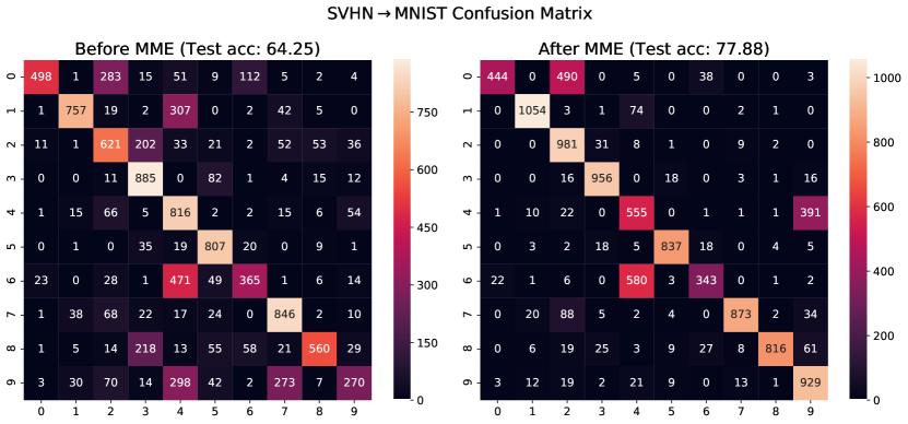
In this section, we attempt to get a sense of the behavior of CLUE versus other methods via visualizations and qualitative examples on the SVHNMNIST shift. Fig. 12 shows confusion matrices of model predictions before (left) and after (right) performing unsupervised adaptation (via MME) at round 0. As seen, MME aligns some classes (eg. 1’s and 9’s) remarkably well even without access to target labels. However, large misalignments remain for some other classes (0, 4, and 6).
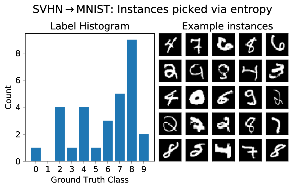
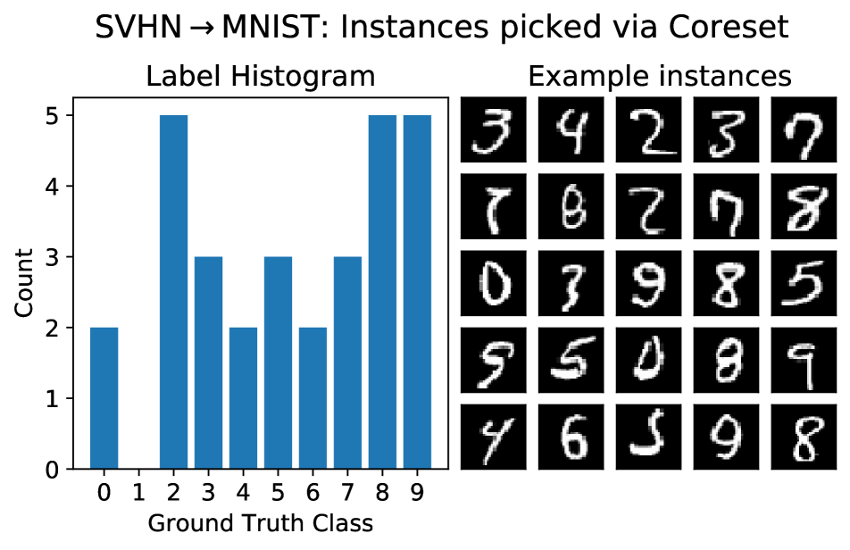
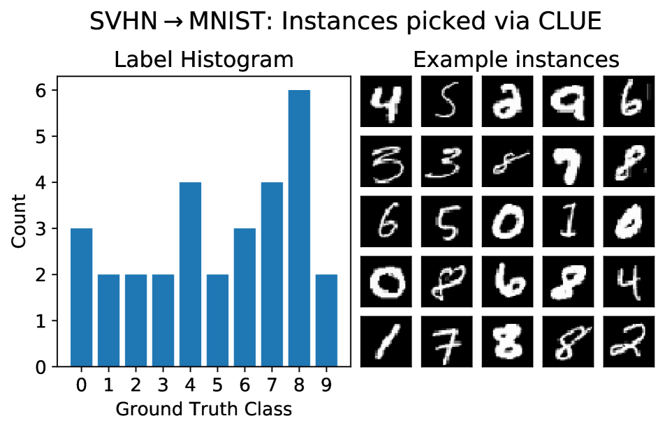
Visualizing selected points. In Fig. 10, we visualize instances selected by three strategies at Round 0 – entropy [52], coreset [42], and CLUE, with . We visualize the ground truth label distribution of the selected instances, as well as qualitative examples. As seen, strategies vary across methods. “Entropy” tends to pick a large number of 8’s, and selects high-entropy examples that (on average) appear challenging even to humans. “Coreset” tends to have a wider spread over classes. CLUE appears to interpolate between the behavior of these two methods, selecting a large number of 8’s (like entropy) but also managing to sample atleast a few instances from every class (like coreset).
t-SNE visualization over rounds. In Fig. 11, we illustrate the sampling behavior of CLUE over rounds via t-SNE [30] visualizations. We follow the same conventions as Fig.3 of the main paper, and visualize the logits of a subset of incorrect (large, opaque circles) and correct (partly transparent circles) model predictions on the target domain, along with instances sampled via CLUE. We oversample incorrect target predictions to emphasize regions of the feature space on which the model currently underperforms. Across all four stages, we find that CLUE samples instances that are uncertain (often present in a cluster of incorrectly classified instances) and diverse in feature space. This behavior is seen even at later rounds when classes appear better separated.
6.7 Extended Description of the CLUE Objective
We describe in more detail the CLUE objective presented (Eq. 4) in the main paper. Recall that we seek to identify target instances that are diverse in model feature space. Considering the L2 distance in the CNN representation space as a dissimilarity measure, we quantify the dissimilarity between instances in a set in terms of its variance given by [55]:
| (6) |
A small indicates that a set contains instances that are similar to one other. Our goal is to identify sets of instances that are representative of the unlabeled target set, by partitioning the unlabeled target data into sets, each with small . Formulating this as a set-partitioning problem with partition function , we seek to find the that minimizes the sum of variance over all sets:
| (7) |
where is defined in Eq. 6.
To ensure that the more informative/uncertain instances play a larger role in identifying representative instances, we employ weighted-variance, where an instance is weighted by its informativeness. Let denote the scalar weight corresponding to the instance . The weighted variance [35] of a set of instances is given by:
| (8) | ||||
Considering the informativeness (weight) of an instance to be its uncertainty under the model, given by (defined in Eq. 1 in main paper), we rewrite the set-partitioning objective in Eq. 7 to minimize sum of weighted variance of a set (from Eq. 8):
| (9) | ||||
This, gives us the overall set-partitioning objective for CLUE.
6.8 Full performance plots
For ease of comparison, we presented performance at 3 intermediate sampling budgets in Tables 1 and 2 in the main paper. In Tables 13, 15, 14, we include the full corresponding performance plots for completeness. Results are presented across 3 learning strategies: finetuning (FT) a source model, semi-supervised DA via MME starting from a source model, and semi-supervised DA via DANN starting from a source model. As is common in active learning, we present results as learning curves, and report performance means and 1 standard deviation over 3 experimental runs via shading.
6.9 Future Work
Our work suggests a few promising directions of future work. First, one could experiment with alternative uncertainty measures in CLUE instead of model entropy, including those (such as uncertainty from deep ensembles) that have been shown to be more reliable under a dataset shift [46]. Further, one could incorporate specialized model architectures from few-shot learning [6, 40] to deal with the label sparsity in the target domain. Finally, while we restrict our task to image classification in this paper, it is important to also study active domain adaptation in the context of related tasks such as object detection and semantic segmentation.