The fate of the false vacuum: Finite temperature, entropy and topological phase in quantum simulations of the early universe

Abstract

Despite being at the heart of the theory of the “Big Bang” and cosmic inflation, the quantum field theory prediction of false vacuum tunneling has not been tested. To address the exponential complexity of the problem, a table-top quantum simulator in the form of an engineered Bose-Einstein condensate (BEC) has been proposed to give dynamical solutions of the quantum field equations. In this paper, we give a numerical feasibility study of the BEC quantum simulator under realistic conditions and temperatures, with an approximate truncated Wigner (tW) phase-space method. We report the observation of false vacuum tunneling in these simulations, and the formation of multiple bubble ’universes’ with distinct topological properties. The tunneling gives a transition of the relative phase of coupled Bose fields from a metastable to a stable ’vacuum’. We include finite temperature effects that would be found in a laboratory experiment and also analyze the cut-off dependence of modulational instabilities in Floquet space. Our numerical phase-space model does not use thin-wall approximations, which are inapplicable to cosmologically interesting models. It is expected to give the correct quantum treatment including superpositions and entanglement during dynamics. By analyzing a nonlocal observable called the topological phase entropy (TPE), our simulations provide information about phase structure in the true vacuum. We observe a cooperative effect in which the true vacua bubbles representing distinct universes each have one or the other of two distinct topologies. The TPE initially increases with time, reaching a peak as the multiple universes are formed, and then decreases with time to the phase-ordered vacuum state. This gives a model for the formation of universes with one of two distinct phases, which is a possible solution to the problem of particle-antiparticle asymmetry.

I Introduction

The evolution of the early universe described by inflation is now a standard model of cosmic evolution. This theory is widely accepted because of the observational evidence including the cosmic microwave background radiation (CMB) detected in all directions. This evidence points to a “Big Bang” origin as the beginning of the Universe. One of the building blocks is a quantum field theory (QFT) model that explains the origin of the early universe and the observed temperature fluctuations in the CMB. These effects originated in Coleman’s theory of quantum tunneling of a scalar quantum field in an initially metastable vacuum (Coleman, 1977; Callan and Coleman, 1977). The validity of the thin-wall approximations used in this theory and later variations are not verified. Quantum field models are exponentially complex and impossible to solve directly.

It is clearly not possible to repeat the start of the universe, so it has been proposed to verify the solutions experimentally. Such experiments would effectively be an analog quantum computer for the scalar field dynamics of the universe. Here we note that the geometry should be multi-mode and have no boundaries, to allow free-space nucleation. The proposal for a suitable quantum analog computer uses a two-species Bose-Einstein condensate (BEC) experiment in a one-dimensional uniform ring configuration, similar to those studied in several laboratories (Guo et al., 2020; Hopkins et al., 2004; Bell et al., 2016). The Bose-Einstein condensate has a modulated coupling between two spin components, which creates a local minimum in the effective phase potential. This allows an experimental study of models of false vacuum quantum tunneling in relativistic scalar field theories, with an engineered scalar field potential.

It is essential to also model the quantum simulator itself. Firstly, this provides insight into the quantum equations themselves, even if only in an approximation. Secondly, it is necessary to understand the performance of the BEC quantum simulator, and its realization in the laboratory as far as possible. In this paper, we employ numerical phase-space methods to simulate the quantum dynamics of the BEC quantum simulator under the conditions of laboratory experiments for up to $1024$ modes. Earlier analyses have verified a false vacuum tunneling, but have not accounted for the effects of finite temperatures and Floquet instabilities in such experiments. Our results show that a momentum cutoff is essential, and that a low initial temperature is required.

A feature of this scalar field model is the existence of a spontaneously broken discrete phase symmetry. This leads to nonlocal topological effects, which are uncovered using phase-unwrapping image processing analysis on the data. There are two distinct types of quantum vacua created with opposite phases. These are locally identical but globally distinct. Similar models have been employed as possible explanations of particle-antiparticle asymmetry (Sakharov, 1991; Zel’dovich et al., 1974; Kibble, 1980). We show that such global topological effects can be quantified using the concept of an observational phase entropy, which can both increase and decrease with time.

Each true vacuum created from the decay of metastable vacua can expand into a separate “universe” with different topological phases, creating domains of vacuum with boundaries. The result of nucleation includes the tunneling rate, the fluctuations in density and temperature, and the collision of domain walls. All play an important role in the physical nature of the resulting universe formed. However, theoretical work so far relies on a number of assumptions which have not been tested in an experiment. False vacuum decay in zero space dimensions has been recently simulated using a quantum computer (Abel and Spannowsky, 2020), but this uses many orders of magnitude fewer qubits than are needed in a spatial model. Here we simulate Coleman’s original model, including multi-mode spatial effects, although without the gravitational effects required in a full cosmological theory.

The present paper describes a numerical simulation, whose purpose is to evaluate the feasibility of an experiment and to predict likely outcomes. We use the most successful dynamical phase-space representation for long times, which is the truncated Wigner (tW) approximation to QFT (Drummond and Hardman, 1993; Steel et al., 1998). This uses a $1/N$ expansion for $N$ bosons, and has had previous success in first-principles predictions of quantum dynamics in bosonic quantum fields. It gives correct predictions of tunneling in small bosonic quantum systems with shallow potentials, by comparison to exact number state and positive-P representation methods (Kinsler and Drummond, 1991). Cosmological models also employ relatively flat potentials (Linde, 1982), so this is not unrealistic.

Previous work analyzed quantum bubble nucleation using a ⁴¹K BEC interferometer (Opanchuk et al., 2013; Fialko et al., 2015, 2017) at zero temperature. This proposed a condensate containing atoms of the same element with two spin components coherently coupled by a microwave field. The coupled BEC is initialized by a Rabi rotation into a metastable state, which decays into a stable state through quantum tunneling. The transition of the BEC from a metastable to a stable state is an ideal experiment for the investigation of Coleman’s original idea. It simulates the relativistic scalar field as a relative phase between the spin components, with the speed of light represented by the speed of sound in the BEC. A related system has been studied using the presence of a seeded vortex within the condensate to initiate false vacuum decay (Billam et al., 2019).

Here we treat a finite-temperature theory, as will occur in a real experiment. We utilize a variation of the Bogoliubov method (Bogolubov, 1947) for treating the quantum initial state, which employs a nonlinear chemical potential to eliminate divergences in the Bogoliubov theory (Ng et al., 2018). We calculate the effects of thermal noise on vacuum tunneling using the truncated Wigner approximation, which has given successful quantum coherence predictions (Drummond and Hardman, 1993; Corney et al., 2006, 2008; Egorov et al., 2011; Drummond and Opanchuk, 2017; Opanchuk et al., 2019). We show that finite temperatures can enhance tunneling, and study how tunneling rates are modified at different initial laboratory temperatures. These results include a momentum cutoff to eliminate Floquet instabilities, and we show that a cutoff is essential by analyzing the effects of changing the cutoff.

We also treat the dynamics and time-evolution of the observable topological phase entropy, which has an intuitive, understandable interpretation. Tunneling events that form the vacuum are disordered, leading to a peak entropy as time evolves. The entropy nearly reaches the maximum possible for an appropriate choice of space and phase bins. As a result, there is a predicted dynamical reduction with time in the topological entropy, as true vacuum domains are formed. The final vacuum state is more ordered, since the false vacuum is unoccupied. Domain-wall formation is minimized at low temperatures, which is important for cosmological interpretations (Zel’dovich et al., 1974), since it is known that high-temperature domain-wall formation can lead to anomalous CMB effects.

II Quantum state representation and Hamiltonian

II.1 Field equations

Bosonic quantum fields with internal degrees of freedom (Guralnik et al., 1964; Higgs, 1964; Englert and Brout, 1964) are used to describe the Higgs sector in the standard particle model. Global symmetries of the Hamiltonian are broken while creating the low-energy ground state or vacuum. The observation of the Higgs particle makes this an important fundamental concept.

The theory of a metastable or ’false’ vacuum was developed by Coleman (Coleman, 1977; Callan and Coleman, 1977). This used a simpler model, treating the fundamental quantum dynamics of a scalar quantum field with non-derivative self-interactions and a Lagrangian density (using a $+---$ metric) of:

$$\mathcal{L}=\frac{1}{2}\partial_{\mu}\phi\partial^{\mu}\phi-U\left(\phi\right).$$ (1)

The local field potential was defined to have two spatially homogeneous, locally stable equilibrium states, $\phi=\phi_{+}$ and $\phi=\phi_{-}$. The first of these has a higher energy, with $U\left(\phi_{+}\right)>U\left(\phi_{-}\right)$. This is unstable to quantum corrections, and is expected to decay to the true vacuum, $\phi_{-}.$ A characteristic predicted to occur in such decays is that a true vacuum is formed by quantum tunneling at a particular space-time point, and subsequently grows at the speed of light.

The dynamics of the evolution of the system is described by Heisenberg field equations of form:

$$\partial_{\mu}\partial^{\mu}\hat{\phi}+U^{\prime}\left(\hat{\phi}\right)=0.$$ (2)

The fact that these are operator equations makes them effectively insoluble, apart from approximations. Even if all the eigenstates were known, as in some one-dimensional theories, there are exponentially many terms (Yurovsky et al., 2017) in an expansion of generic initial states.

Coleman analyzed a scalar quantum field theory of how such a true vacuum would arise, given an initial metastable state. This model also predicted the formation of individual early universe ’bubbles’. Such theories can be extended to include gravitational effects, and have been used as a theory of the early universe (Guth, 1981). In these, the scalar field is renamed the inflaton field, and decay to a true vacuum causes an inflationary expansion (Linde, 1982), creating the ’Big Bang’. More recent cosmological studies often focus on post-inflationary events (Musoke et al., 2020), which are less sensitive to quantum fluctuations.

The observation of the Higgs particle and evidence for CMB density fluctuations, confirms the importance of such quantum field theory models. Yet the original false vacuum energies are thought to be many orders of magnitude greater than any possible experiment, possibly $\sim 10^{15}\mathrm{GeV}$ (Linde, 1982). The original event is also hidden from direct observation. In addition to such experimental problems, the quantum field theory itself is exponentially complex, and cannot be solved exactly. As a result, the theory has mainly been analyzed using classical or perturbative approximations (Mukhanov et al., 1992). The inclusion of general relativistic effects further complicates the analysis.

It is important to have a better understanding of at least the simplest quantum field theory models. A feature of the model we use is that it possesses a spontaneously broken discrete symmetry, which is known to provide a potential solution to the particle-antiparticle asymmetry problem (Zel’dovich et al., 1974). Qualitative analysis of domain-wall formation at high initial temperatures has led to objections to this idea (Kibble, 1980), related to CMB spectral observations. A full quantum dynamical treatment of the location of domain-walls is needed. Our simulations show that at high temperatures domain walls are prevalent. However, at low temperatures, domain walls are restricted to universe boundaries where they appear less likely to cause inhomogeneities in the CMB spectrum. Observing domain walls in an experimental setting would help to verify or refute this analysis.

II.2 Approximations and interpretation

Since digital quantum computers are orders of magnitude too small, we propose to solve the equations using an analog quantum computer: a laboratory BEC quantum simulator. In order to obtain insight into the expected performance of the simulator, the dynamics of the BEC system will be solved numerically, but with approximations. Here, we give an outline of those approximations, explaining where they will be expected to hold, and also discuss the interpretation of the simulations.

An interesting consequence of all quantum models for the universe is that the entire universe is described as a single quantum state: there is no external observer. Quantum measurement theory in the conventional Copenhagen model requires an observer to collapse the wave-function. As a result, there are foundational problems in interpreting the wave-function itself. This leads to the question of what can one identify in the simulation that will correspond to a universe?

The numerical simulations of this paper give predictions of the dynamics of the wave function for a model of the universe according to a Hamiltonian treatment. As such the averages taken over the simulations provide the ensemble predictions for the laboratory experiment if repeated many times. An interesting question is whether or how a particular laboratory realization can relate to a particular dynamical trajectory.

We use a mapping of the wave-function to a Wigner field distribution but with a simpler, approximate time-evolution equation which ensures a positive Wigner distribution throughout the dynamics. In this truncated Wigner (tW) model, stochastic equations are written for complex amplitudes $\alpha_{k}$ that represent modes $k$. These equations are solved numerically, the quantum noise being modeled stochastically. There is a direct correspondence between the observable experimental moments of the field quadratures and the moments of the real and imaginary parts of $\alpha_{k}$. The measured quantity of interest is the particle number which, once operator ordering is taken into account, corresponds to $|\alpha_{k}|^{2}$ up to an error of order $\sim 1$. The values of $|\alpha_{k}|^{2}$ encountered in the simulations are macroscopic, and hence the difference between operator and simulation moments is negligible. In this sense, a probabilistic interpretation is possible, where the individual complex amplitudes trajectories correspond to an individual realization. Vacuum fluctuations may be considered as real events, and no additional collapse mechanism is required, as discussed in greater detail in Section (IV).

The dynamics of the tW distribution is approximate. Even though the local evolution errors when using the tW method are of order $1/N$ where $N$ is the number of particles in each mode, these may grow during time-evolution to create macroscopic errors at later times (Drummond and Kinsler, 1989; Kinsler and Drummond, 1991; Sinatra et al., 2002; Deuar and Drummond, 2007). Such errors can increase during quantum tunneling. The tW method cannot describe the formation of macroscopic superposition states (Yurke and Stoler, 1986; Budroni et al., 2015; Kovachy et al., 2015; Opanchuk et al., 2016; Rosales-Zárate et al., 2018) , or predict certain macroscopic Bell violations (Thenabadu et al., 2020), because such states cannot be described by a positive Wigner function. Quantum squeezing and entanglement can be described however.

As it is a feasibility study, we do not give exact results, because the quantum simulator experiment is intended to do this. Nevertheless, it is important to ask how reliable the tW phase-space method is. The tW distribution has been used to predict both squeezing and entanglement in systems of large particle number. Comparisons have been made of tW and exact positive-P methods for the dynamics of quantum squeezing in solitons (Drummond and Hardman, 1993; Opanchuk and Drummond, 2017; Steel et al., 1998), with excellent agreement between both methods and with experiments (Rosenbluh and Shelby, 1991; Corney et al., 2006, 2008). There is also good experimental agreement for large-scale quantum BEC interferometry, where fringe visibility decoherence times have been accurately predicted. In this regime, quantum entanglement in the form of Schrodinger’s quantum steering has been inferred based on the simulations, for states of up to 40,000 atoms (Opanchuk et al., 2019).

Other studies treated quantum tunneling in driven non-equilibrium systems, which showed agreement between tW and exact methods for shallow tunneling potentials (Drummond and Kinsler, 1989; Kinsler and Drummond, 1991). This agreement disappeared for deeper potential wells, which is more likely to lead to macroscopic superposition states requiring negative Wigner distributions. Another quantum field system with metastable behavior is the quantum solitonic breather (Yurovsky et al., 2017; Opanchuk and Drummond, 2017), for which tW methods have shown good agreement with conservation laws (Drummond and Opanchuk, 2017) and both exact positive-P representation and integrable methods (Ng et al., 2019; Marchukov et al., 2020) during the early stages of breather relaxation.

While Coleman’s original model proposed a deep potential, the models currently favored by many cosmologists do not. Instead, a shallow potential is thought to be more realistic in an inflationary universe (Linde, 1982). As a result, it is reasonable to use a relatively flat quantum field internal potential, with a large particle number. In this regime, the numerical simulation methods used here appear reliable. Nevertheless, owing to the long time-scales involved - and possible error growth (Kupiszewska and Rzazewski, 1990; Kinsler et al., 1993) - the main goal here is an experiment, regarded as an early universe quantum simulation.

II.3 Two-species Hamiltonian

For a BEC system having two occupied hyperfine levels with mass $m$, the Hamiltonian of the coupled field system includes an s-wave scattering potential (Leggett, 2001). It is important in our model that there is a strong mixing between the two spin species, without a phase separation. This requires that the inter-species interaction is minimized, and is assumed to be zero here. There will be losses due to spin-changing inelastic collisions, but these dissipative effects are neglected. The size of such effects is not known for the ⁴¹K Feshbach resonance of interest. This provides a limitation on the accessible tunneling times, since the atoms must tunnel before they are absorbed.

A general two-species Hamiltonian includes both intra and inter-species scattering. The inter-species scattering length is often close to the intra-species one, since differences in nuclear spin orientation do not strongly perturb inter-atomic forces. However, this can change dramatically at a magnetic Feshbach resonance. The required tuning of the s-wave scattering interactions can therefore be achieved with the external magnetic field chosen so that cross-species scattering is suppressed. This is possible in ⁴¹K, as well as in other isotopes like ⁷Li.

In these cases, near the Feshbach resonance, one can write the Hamiltonian as

$$\hat{H}=\stackrel{{\scriptstyle[}}{{j}}=1]{2}{\sum}\hat{H}_{j}+\hat{H}_{c}.$$ (3)

Here, writing $\hat{\Psi}_{j}\equiv\hat{\Psi}_{j}\left(\mathrm{x},t\right)$ for brevity for the $j$-th Bose field, the individual spin-species Hamiltonians are

$$\hat{H}_{j} = \int d\mathrm{x}\left(-\hat{\Psi}_{j}^{\dagger}\frac{\hbar^{2}\nabla^{2}}{2m}\hat{\Psi}_{j}+\frac{g}{2}\hat{\Psi}_{j}^{\dagger 2}\hat{\Psi}_{j}^{2}\right),$$ (4)

and the microwave coupling Hamiltonian, $\hat{H}_{c}$, is

$$\hat{H}_{c} = -\nu\left(t\right)\int d\mathrm{x}\left(\hat{\Psi}_{2}^{\dagger}\hat{\Psi}_{1}+\hat{\Psi}_{1}^{\dagger}\hat{\Psi}_{2}\right).$$ (5)

The components $\hat{\Psi}_{j}$ are the coupled field operators corresponding to different nuclear spin states, and the subscripts $j,k=1,2$ are the spin indices. These operators have commutation relations $\left[\hat{\Psi}_{j}\left(\mathrm{x},t\right),\hat{\Psi}_{k}^{{}^{\prime}}\left(\mathrm{x}^{\prime},t\right)\right]=0$ and $\left[\hat{\Psi}_{j}\left(\mathrm{x},t\right),\hat{\Psi}_{k}^{{}^{\prime}\dagger}\left(\mathrm{x}^{\prime},t\right)\right]=\delta_{jk}\delta_{M}(\mathrm{x}^{\prime}-\mathrm{x})$. Here $\delta_{M}(\mathrm{x}^{\prime}-\mathrm{x})$ is a restricted delta function (Opanchuk and Drummond, 2013) that includes a momentum cutoff, restricting the field to a lattice for numerical simulation.

The coefficient $g$ is the s-wave scattering interacting strength between the atoms, which for a three-dimensional system, $g_{3D}$, is given by:

$$g_{3D}=\frac{4\pi\hbar^{2}a}{m},$$ (6)

where $a$ is the s-wave scattering length.

If the atoms are confined by a transverse harmonic trap with frequency $\omega_{\perp}$, where the transverse trapping energy $\hbar\omega_{\perp}$ is much higher then the thermal energy, the Bose gas reaches a one-dimensional regime (Deuar et al., 2009). In this regime, the atoms are confined tightly within an effective s-wave cross-section $A_{s}=2\pi(l_{\perp})^{2}$, where $l_{\perp}=\sqrt{\hbar/m\omega_{\perp}}$ is the transverse harmonic oscillator length (Olshanii, 1998; Kheruntsyan et al., 2005; Bouchoule et al., 2012). The coefficient $g$ for a one-dimensional system is hence expressed as $g=g_{3D}/A_{s}$, which gives:

$$g=\frac{2\hbar^{2}a}{ml_{\perp}^{2}}=2\hbar a\omega_{\perp}.$$ (7)

We neglect microwave spontaneous emission effects, as these are very weak for such microwave transitions.

II.4 Stephenson-Kapitza pendulum term

The coupling $\nu$ describes a microwave field that rotates the nuclear spin by resonantly coupling two hyperfine levels with a frequency separation of $\Omega_{HF}$ in the external magnetic field. This is modulated in time in order to induce metastability using Stephenson’s concept of a modulated pendulum (Stephenson, 1908; Stoker, 1950; Kapitza, 1965a), later popularized by Kapitza (Kapitza, 1965a). The depth of the field potential in the metastable state is determined by the dimensionless variable $\delta$.

We work in a rotating frame such that this energy separation is removed from the Hamiltonian, using a different reference energy for each spin component. Here $\nu\left(t\right)$, the coupling strength between the spin components, is modulated (Stephenson, 1908; Stoker, 1950; Kapitza, 1965a, b; Ibrahim, 2006) as a sinusoidal time-dependent variable with an additional modulation frequency $\omega$, so that

$$\nu\left(t\right)=\nu+\delta\hbar\omega\cos\omega t.$$ (8)

Provided the modulation is at a high frequency, this Hamiltonian is equivalent to the Coleman model of a relativistic scalar quantum field with an engineered quartic potential. Here the phonon velocity corresponds to the speed of light (Opanchuk et al., 2013; Fialko et al., 2017). Modulation amplitudes are relatively large, so that the excitation is nearly bichromatic (Freedhoff and Chen, 1990; Zhu et al., 1990), or double-sideband.

The result of including this term is an engineered potential $U\left(\phi_{a}\right)$ for an effective scalar field $\phi_{a}$ which physically is the phase difference between the two co-existing Bose-Einstein condensates with phases $\phi_{j}$. We define the atomic phase difference as $\phi_{a}=\phi_{1}-\phi_{2}-\pi$, so that the false vacuum is at $\phi_{a}=0$ and the true vacua are at $\phi_{a}=\pm\pi.$ In the limit of strong particle-particle repulsion, this obeys the relativistic field equation (2), where the speed of light, $c$, is replaced by the phonon velocity, $c=\sqrt{g\rho_{0}/m}$ in the BEC.

The potential equation is given by (Fialko et al., 2017):

$$U\left(\phi_{a}\right)=\omega_{0}^{2}\cos\left(\phi_{a}\right)\left[1-\frac{\lambda^{2}}{2}\sin^{2}\left(\phi_{a}\right)\right],$$ (9)

where $\omega_{0}=2\sqrt{\nu g\rho_{0}}/\hbar$ and $\lambda=\delta\sqrt{2g\rho_{0}/\nu}.$ This potential can be varied by the experimentalist, and is best understood in a dimensionless form described later.

It is known that instabilities can form in this model at too low a modulation frequency. This is due to coupling between effects caused by the modulation frequency and high-frequency phonon modes (Braden et al., 2018, 2019). Such effects therefore require the use of high enough modulation frequencies to move the instability region above any physical cutoff in momentum.

We will assume that there is a physical mechanism to remove high-momentum phonon modes. An example of this would be the use of a spatially modulated potential to introduce a band-gap. A second possibility is the use of a swept modulation frequency to reduce parametric gain by changing the unstable momenta. Ultimately, as pointed out by earlier workers, the inverse scattering length provides an intrinsic cutoff, ultimately at $1/a$.

An experimental mechanism to achieve this is via an optically modulated trap potential. Instabilities were not observed in our previous numerical simulations, due to the use of a finite lattice that includes a momentum cutoff. An analysis of modulational instabilities in experiments with larger numbers of modes and higher phonon momenta is given in the Appendix, where typical parameters are presented.

We conclude that such instabilities are generally present, but can be suppressed in the proposed experiment by using high enough modulation frequencies combined with a momentum cutoff, as shown in Fig (1).

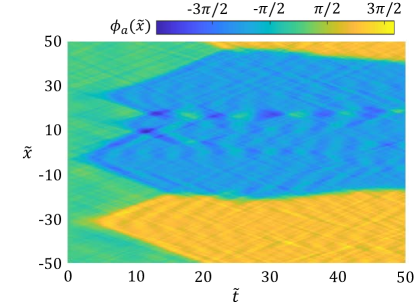
Figure 1: Example of a single trajectory decay to a true vacuum, starting in a $1D$ false vacuum initialized with finite temperature effects. The false vacuum is seen to decay to two distinct topological phases for the true vacuum, indicated by yellow and light-blue regions. The bubbles of true vacuum expand in space until they meet each other. At long time scales, the universes are separated by domain walls of false vacuum, indicated by the color green. Dimensionless parameters are $\tau=10^{-5}$, $\widetilde{\nu}=7\times 10^{-3}$, $\lambda=1.2$, $\widetilde{\omega}=50$ and $\widetilde{\rho}=200$.

III Initial state at finite temperature

Our initial state includes quantum and thermal fluctuations. We combine the Bogoliubov method (Bogolubov, 1947) with the Wigner representation, so that both the initial thermal excitations and vacuum noise are taken into account. In this approximation, the system is assumed to have a macroscopic condensate mean population $N_{c}$ with density $\rho_{c}$ for one of the spin indices, say $j=1$. Experimentally, this is produced using evaporative cooling methods (Cornell and Wieman, 2002; Ketterle and Van Druten, 1996; Bradley et al., 1997).

The ground state field operator $\hat{\Psi}_{1}$ is nearly equal to the square root of the condensate density, $\sqrt{\rho_{c}}$, which is assumed constant over the ring. This is valid for typical ultra-cold BEC experiments below threshold, provided trapping potential noise is small. There are zero momentum divergences in applying the Bogoliubov expansion to finite systems, which are removed here using a nonlinear chemical potential (Ng et al., 2018).

Initially, the microwave coupling $\nu$ is turned off, and the second spin species operator $\hat{\Psi}_{2}$ is in the vacuum state. The BEC is prepared in a single species condensate with one spin component populated at a temperature $T$. While it is possible to achieve temperatures well below the condensate critical temperature, these are still not at zero temperature. The condensate has thermal phonon excitations, which can change the tunneling time. These also induce phase fluctuations and finite temperatures in the effective scalar field.

This is expected to give modified tunneling compared to a metastable quantum field without extra noise. Since the exact quantum state prior to the Big Bang is not known precisely, our goal here is to determine the effect of thermal noise on a laboratory experiment. Even this may not capture the full effects of evaporative cooling, which is a complex dynamical process (Drummond and Corney, 1999).

III.1 Nonlinear chemical potential

To model a finite temperature experiment, we assume that the initial density matrix is in a grand canonical ensemble $\hat{\rho}_{GC}$ at temperature $T$ for $j=1$, and a vacuum state for $j=2$, so that:

$$\hat{\rho}_{GC}=e^{-\beta\hat{K}}\left|0\right\rangle\left\langle 0\right|_{2}.$$ (10)

Here $\hat{K}$ is the ’Kamiltonian’ , which includes a chemical potential to give a finite particle number in the thermal state, so that

$$\hat{K}=\hat{H}-\mu\left(\hat{N}\right),$$ (11)

where $\mu\left(\hat{N}\right)$ is the chemical potential for an initial population $\hat{N}$ in one of the spin configurations. This can be any nonlinear function of $\hat{N}$ (Ng et al., 2018), so that, including terms up to second order

$$\mu\left(\hat{N}\right)=\mu_{1}\hat{N}+\frac{\mu_{2}}{2}:\hat{N}^{2}:.$$ (12)

The chemical potential has no effect on the dynamics if $\nu=0$, since $\left[\hat{H},\mu\left(\hat{N}\right)\right]=0$. Such a nonlinear chemical potential is useful for describing thermal fluctuations in a BEC. The utility of this approach is that on linearizing the total Kamiltonian, $\hat{K}$, the zero frequency divergence of the Bogoliubov expansion (Bogolubov, 1947) is eliminated with an appropriate choice of the quadratic coefficient $\mu_{2}$.

To allow an expansion around a well-defined coherent state phase, we suppose that $\hat{\rho}$ is an ensemble average of condensates $\hat{\rho}\left(\phi_{c}\right)$ with a coherent phase $\phi_{c}$, so that:

$$\hat{\rho}_{GC} =\frac{1}{2\pi}\int d\phi\hat{\rho}\left(\phi_{c}\right)\,.$$ (13)

This ensemble corresponds to a number-averaged ensemble of states with Poissonian number fluctuations around $N_{c}$, which is more realistic than using a fixed particle number. The actual number fluctuations in experiments are often super-Poissonian, and these additional number fluctuations can be included if required.

For number-conserving interferometric measurements of relative phase, the initial coherent phase $\phi_{c}$ is irrelevant. All phase choices give identical observables. It is therefore sufficient to include a single member of the phase ensemble with $\phi_{c}=0$, following standard methods from laser physics (Glauber, 1963; Louisell, 1973; Drummond and Hillery, 2014). There are other techniques for obtaining convergent Bogoliubov expansions (Gardiner, 1997; Boccato et al., 2019). These generally involve operator expansions having non-standard commutators, and do not readily permit Wigner phase-space expansions.

III.2 Regularized Bogoliubov theory

The grand canonical Hamiltonian, $\hat{K}$, is obtained from a Bogoliubov expansion (Bogolubov, 1947; Fetter, 1972; Lewenstein and You, 1996) of the single-species field operator at time $t=0$, assuming a condensate phase of $\phi_{1}=0$. This is given by

$$\hat{\Psi}_{1}(x,0)=\psi_{c}+\delta\hat{\Psi}_{1}.$$ (14)

Here $\psi_{c}=\sqrt{\rho_{c}}$, which is the initial condensate density, and the field fluctuations are expanded as a sum over phonon momenta $k$:

$$\delta\hat{\Psi}_{1} =\frac{1}{\sqrt{L}}\underset{k}{\sum}\left[u_{k}\hat{b}_{k}e^{ikx}-v_{k}\hat{b}_{k}^{\dagger}e^{-ikx}\right].$$ (15)

For a complete unitary transformation, all modes must be included, including the zero-momentum mode. Next, we introduce the condensate quadrature operator $\hat{P}$ as

$$\hat{P}\equiv\int d\bm{x}\left(\delta\hat{\Psi}_{1}+\delta\hat{\Psi}_{1}^{\dagger}\right)/\sqrt{2}\,.$$ (16)

The number operator $\hat{N}$ can be written to second order in the quantum field fluctuations, giving

$$\hat{N}=N_{c}+\hat{P}\sqrt{2\rho_{c}}+\int d\bm{x}\delta\hat{\Psi}^{\dagger}\delta\hat{\Psi}\,.$$ (17)

Expanding the grand canonical Hamiltonian in $\delta\hat{\Psi}_{1}$, the choice of $\mu_{1}=0$ and $\mu_{2}=g/L$ eliminates all first order terms as well as terms in $\hat{P}^{2}$, which would cause phase divergences and unphysical phase diffusion in equilibrium. The resulting convergent Bogoliubov expansion has $u_{0}=1$ and $v_{0}=0$ for the zero-momentum terms with $k=0$, rather than the divergent expression found in the standard expansion.

The mode coefficients of the single-species field for $k\neq 0$ are expressed in terms of the excitation energy $\epsilon_{k}$ and the free-particle energy $E_{k}$, as

$$u_{k} =\frac{\epsilon_{k}+E_{k}}{2\sqrt{\epsilon_{k}E_{k}}},$$

$$v_{k} =\frac{\epsilon_{k}-E_{k}}{2\sqrt{\epsilon_{k}E_{k}}},$$ (18)

where $E_{k}=\hbar^{2}k^{2}/\left(2m\right)$ is the free-particle energy and

$${\color[rgb]{1,0,0}{\normalcolor\epsilon_{k}=\sqrt{E_{k}(E_{k}+2g\rho_{c})}}}$$ (19)

is the excitation energy. Due to periodic boundary conditions on a ring trap, the allowed values of momenta are

$$k_{j}=\frac{2\pi j}{L}\,,$$ (20)

for $j=\left(1-M\right)/2,\ldots\left(M-1\right)/2$ for $M$ momentum modes, assuming an odd mode number. The resulting effective Kamiltonian describing thermal excitations of the BEC is given by

$$\hat{K}^{(2)}=\sum\epsilon_{k}\hat{b}_{k}^{\dagger}\hat{b}_{k}\,.$$ (21)

Here, the phonon operators $\hat{b}_{k}^{\dagger},\hat{b}_{k}$ describe the creation and annihilation of a quasi-particle in an excited state $k$. The resulting excitation in each mode with $k\neq 0$ is a propagating phonon. This expansion is particularly useful for the finite temperature system we are interested in here. Phonon excitations with $k\neq 0$ are populated according to the bosonic thermal distribution,

$$\langle\hat{n}_{k}\rangle =\langle\hat{b}_{k}^{\dagger}\hat{b}_{k}\rangle\equiv n_{k}=\frac{1}{\mathrm{exp}(\beta\epsilon_{k})-1},$$ (22)

where $\beta=1/k_{B}T$.

For $k=0$, we assume a vacuum state with $n_{0}=0$, since this operator cannot be coupled to an energy exchange process, owing to number conservation. This choice gives Poissonian number fluctuations. As discussed above it may be necessary in modeling experiments to include larger number fluctuations due to technical noise occurring in the evaporative cooling process.

After the initial preparation, a microwave pulse is used to rotate the Bose gas occupations so that the two spin species have an equal occupation, which is equivalent to a linear beam-splitter. We denote $\hat{\Psi}_{j}^{\prime}(x,0)$ as the initial quantum fields after the BEC is split into the two states. The two initial spin states after rotation have equal density $\rho_{0}=\rho_{c}/2$ and a relative phase of $\pi$.

This corresponds to a rotation matrix acting on the quantum fields $\hat{\Psi}_{1}$ and $\hat{\Psi}_{2}$:

$$\left(\begin{array}[]{c}\hat{\Psi}_{1}^{\prime}\\ \hat{\Psi}_{2}^{\prime}\end{array}\right) =\left(\begin{array}[]{cc}\mathrm{cos}\frac{\theta}{2}&-ie^{-i\phi}\mathrm{sin}\frac{\theta}{2}\\ -ie^{i\phi}\mathrm{sin}\frac{\theta}{2}&\mathrm{cos}\frac{\theta}{2}\end{array}\right)\left(\begin{array}[]{c}\hat{\Psi}_{1}\\ \hat{\Psi}_{2}\end{array}\right),$$ (29)

where $\theta=\pi/2$ and $\phi=-\pi/2$. The system is then assumed to evolve according to the Hamiltonian (3) with a c.w. microwave coupling field present. This carrier has an appropriate phase relationship with the microwave pulse field so that the quantum system is initially in the metastable high energy state.

III.3 Dimensionless parameters

The equation of motion and quantum operators can be transformed into dimensionless form by introducing dimensionless time, distance, and frequency:

$$\widetilde{t} =t\omega_{0}$$

$$\widetilde{x} =x/x_{0}=x\omega_{0}/c$$

$$\tilde{\omega} =\omega/\omega_{0}.$$ (30)

The speed of sound in a weakly interacting BEC is given by $c=\sqrt{g\rho_{0}/m}$, and the initial temperature of quantum degeneracy is $T_{d}$ (Kheruntsyan et al., 2003). We define a characteristic length, temperature and frequency as:

$$x_{0} =\frac{\hbar}{2\sqrt{m\nu}}$$

$$T_{d} =\frac{\hbar^{2}\rho_{c}^{2}}{2mk_{B}}$$

$$\omega_{0} =2\frac{\sqrt{\nu g\rho_{0}}}{\hbar}.$$ (31)

The field amplitude in dimensionless coordinates is $\widetilde{\Psi}_{j}=\hat{\Psi}_{j}\sqrt{x_{0}}$, and the density in dimensionless form is given by $\widetilde{\rho}_{0}=\rho_{0}x_{0}$. This gives a characteristic energy scale that is the geometric mean of the mean field energy $g\rho_{0}$ and coupling energy $\nu$, as used previously. The six dimensionless parameters that define the physical system are therefore:

$$\widetilde{\rho}_{0} =\rho_{0}x_{0}$$

$$\widetilde{L} =L/x_{0}$$

$$\tau =T/T_{d}$$

$$\lambda =\delta\hbar\omega_{0}/\sqrt{2}\nu$$

$$\widetilde{\omega} =\omega/\omega_{0}$$

$$\tilde{\nu} =\nu/g\rho_{0},$$ (32)

where $\widetilde{L}$ is the dimensionless length of the simulation, $T$ is the temperature of the initial BEC field with density $\rho_{c}=2\rho_{0}$, and $\lambda$ is the effective depth of the modulation. The corresponding dimensionless Hamiltonian, including the chemical potential, is:

$$\tilde{H}_{j}=\int_{-\tilde{L}/2}^{\tilde{L}/2}d\widetilde{x}\left(-\sqrt{\tilde{\nu}}\tilde{\Psi}_{j}^{\dagger}\tilde{\Psi}_{j}+\frac{\tilde{g}}{2}\tilde{\Psi}_{j}^{\dagger 2}\tilde{\Psi}_{j}^{2}\right)-\frac{\tilde{g}}{2\tilde{L}}\hat{N}_{1}^{2}.$$ (33)

Here $\tilde{g}=1/(2\widetilde{\rho}_{0}\sqrt{\widetilde{\nu}})$, the effective nonlinearity, depends on the other parameters. The chemical potential has no effect on dynamics, and is only required to remove singularities in the linearization of the initial state.

IV Phase-space representations and entropy

To investigate vacuum nucleation at finite temperature, we take both quantum and thermal fluctuations into account. This is achieved by performing stochastic numerical simulations in the Wigner representation of the full quantum model of the two-component BEC system. These numerical simulations are not exact, and indeed there is no exact method known. Such large-scale quantum field calculations are exponentially complex. This lack of an exact solution is the motivation for a quantum simulation experiment. However, we can use stochastic methods to investigate realistic conditions and expected results.

The effect of quantum and thermal fluctuations results in a wide range of nucleation times. Numerical methods which are not limited to short simulation time are desirable to simulate the Coleman theory. Here we choose the truncated Wigner (tW) approach (Wigner, 1932; Drummond and Hardman, 1993; Steel et al., 1998). It has a sampling error that remains well-controlled over a long simulation times. This method gives the first quantum corrections in an $M/N$ expansion (Norrie et al., 2006), were $M$ is the number of modes and $N$ is the number of atoms. To give reliable results, it is therefore necessary that $M/N<<1$. This has been confirmed in comparisons with exact positive-P and complex-P simulations that do not use truncations (Ng et al., 2019; Drummond and Hardman, 1993).

There have been successful predictions of measured quantum squeezing in solitons (Rosenbluh and Shelby, 1991; Drummond et al., 1993; Drummond and Hardman, 1993; Corney et al., 2006, 2008), propagation effects in BEC lattices (Ruostekoski and Isella, 2005) and fringe visibility in finite temperature BEC interferometers (Opanchuk et al., 2019; Steel et al., 1998). These also indicate that the technique is reliable. Hence the tW method should be able to simulate these experiments given a large number of atoms. Truncation errors can build up at long times (Sinatra et al., 2002). This means that the numerical simulations are expected to be correct if tunneling is not too slow. The ultimate goal is an experiment.

Tunneling phenomena are a stringent test of numerical quantum field simulations. Earlier comparisons of truncated Wigner quantum tunneling with exact methods have shown that it is correct for relatively shallow potentials (Drummond and Kinsler, 1989; Kinsler and Drummond, 1991). This is also the regime of most interest in many cosmological models. As a result, we expect that this method will give good indications of the effects of thermal and quantum noise in the regimes of most interest.

Using this approach, the quantum state is represented by a stochastic phase space distribution of trajectories following the Gross-Pitaevskii equation. In a thermal state, the Wigner representation of the initial state has a complex Gaussian distribution. We perform our simulations for a one-dimensional system, whose equation of motion are obtained from (4). A typical example is shown in Fig (1).

IV.1 Wigner representation

We require that the dynamics of the system is evolved quantum dynamically, hence quantum fluctuations must be taken into account. To do this, we transform the phonon operators using the Wigner representation correspondence (Drummond and Hardman, 1993; Steel et al., 1998; Opanchuk and Drummond, 2013; Drummond and Opanchuk, 2017). Since the initial state is approximately Gaussian before phase-averaging, the corresponding initial Wigner representation is also Gaussian (Ruostekoski and Isella, 2005; Isella and Ruostekoski, 2006).

Each initial phonon mode is represented as a complex Gaussian variable, i.e. $\hat{b}_{k}\sim\beta_{k}$ and $\hat{b}_{k}^{\dagger}\sim\beta_{k}^{*}$. Thermal fluctuations are included in the modes with $k\neq 0$. A detailed explanation of how this is obtained using the nonlinear chemical potential method is explained elsewhere (Ng et al., 2018). The Wigner representation of the initial quantum density matrix $\hat{\rho}\left(0\right)$, after evaporative cooling, is a complex Gaussian distribution given by:

$$W\left[\bm{\psi}\right]=W_{1}\left[\psi_{1}\right]W_{2}\left[\psi_{2}\right].$$ (34)

Here, $W_{1}\left[\psi_{1}\right]$ is a representation of a thermal state with finite temperature, and $W_{2}\left[\psi_{2}\right]$ is a vacuum state. These are positive distributions that can be sampled probabilistically, with samples given after evaporative cooling by:

$$\psi_{1} =\psi_{c}+\frac{1}{\sqrt{L}}\underset{k}{\sum}\left(u_{k}\beta_{k}e^{ikx}-v_{k}\beta_{k}^{*}e^{-ikx}\right)$$

$$\psi_{2} =\frac{1}{\sqrt{L}}\underset{k}{\sum}\alpha_{k}e^{ikx},$$ (35)

with $\alpha_{k}$ and $\beta_{k}$ defined as independent complex Gaussian random variables in each vacuum mode and phonon mode respectively. These have mean values such that $\langle\alpha_{k}^{2}\rangle=\langle\alpha_{k}\rangle=0$, $\langle\beta_{k}^{2}\rangle=\langle\beta_{k}\rangle=0$. The only non-vanishing moments are

$$\langle\left|\alpha_{k}\right|^{2}\rangle = \frac{1}{2}$$

$$\langle\left|\beta_{k}\right|^{2}\rangle = n_{k}+\frac{1}{2}.$$ (36)

IV.2 Reduction to dimensionless parameters

In dimensionless form, Eq (35) for the condensate after cooling and before rotation, is given by

$$\widetilde{\psi}_{1} =\widetilde{\psi_{c}}+\frac{1}{\sqrt{\widetilde{L}}}\sum\left(u_{\widetilde{k}}\beta_{\widetilde{k}}e^{i\widetilde{k}\widetilde{x}}-v_{\widetilde{k}}^{*}\beta_{\widetilde{k}}^{*}e^{-i\widetilde{k}\widetilde{x}}\right)$$

$$\widetilde{\psi}_{2} =\frac{1}{\sqrt{\widetilde{L}}}\sum\alpha_{\widetilde{k}}e^{i\widetilde{k}\widetilde{x}},$$ (37)

where $|\widetilde{\psi}_{c}|^{2}=\widetilde{\rho}_{c}=2\widetilde{\rho}_{0}$ is the mean field density of the single-species condensate before rotation. The first term is an inverse Fourier transform of the collective excitations in Wigner representation. The resulting values for $u,v$ are

$$u_{\tilde{k}} =\frac{\widetilde{\epsilon}_{\widetilde{k}}+\widetilde{E}_{\widetilde{k}}}{2\sqrt{\widetilde{\epsilon}_{\widetilde{k}}\widetilde{E}_{\widetilde{k}}}},$$

$$v_{\tilde{k}} =\frac{\widetilde{\epsilon}_{\widetilde{k}}-\widetilde{E}_{\widetilde{k}}}{2\sqrt{\widetilde{\epsilon}_{\widetilde{k}}\widetilde{E}_{\widetilde{k}}}},$$ (38)

where $\widetilde{\epsilon}_{\widetilde{k}}=\epsilon_{k}/\hbar\omega_{0}$ is the Bogoliubov excitation energy in dimensionless form, so that, in dimensionless units:

$$\widetilde{E}_{\widetilde{k}} =\tilde{\nu}\tilde{k}^{2}$$

$$\widetilde{\epsilon}_{\widetilde{k}} =\tilde{\nu}\sqrt{\tilde{k}^{2}\left(\tilde{k}^{2}+\frac{2}{\tilde{\nu}^{2}}\right)}.$$

IV.3 Metastable state generation and detection

Assuming that the thermal phonons effectively behave as a canonical ensemble of free bosons, the thermal fluctuations for $\widetilde{k}\neq 0$ are represented by the complex Wigner amplitude

$$\beta_{\widetilde{k}} =\frac{\eta_{1,\widetilde{k}}}{\sqrt{2\mathrm{tanh}(\widetilde{\epsilon}_{\widetilde{k}}/8\widetilde{\nu}\widetilde{\rho}_{0}^{2}\tau)}},$$ (39)

$$\alpha_{\widetilde{k}} =\frac{\eta_{2,\widetilde{k}}}{\sqrt{2}},$$ (40)

where $\eta_{i,\widetilde{k}}$ is a complex Gaussian noise in dimensionless space, with $\langle\eta_{i,\widetilde{k}}\eta_{j,\widetilde{k}^{\prime}}^{*}\rangle=\delta_{ij}\delta_{\widetilde{k}\widetilde{k}^{\prime}}$ . As a result,

$$\langle|\beta_{\widetilde{k}}|^{2}\rangle =n_{\widetilde{k}}+\frac{1}{2}$$

$$\langle|\alpha_{\widetilde{k}}|^{2}\rangle =\frac{1}{2}.$$ (41)

To create the metastable state described in Coleman theory in our proposed experiment, a radio frequency field with shifted phase of $\pi/2$ is applied to the single-species BEC. This prepares a superposition of initial states $|1\rangle$ and $|2\rangle$, where the two-component condensate corresponds to the initial metastable state, together with finite temperature thermal fluctuations.

We denote $\widetilde{\psi}_{1,0}^{{}^{\prime}}$ and $\widetilde{\psi}_{2,0}^{{}^{\prime}}$ as the initial Wigner fields after the BEC is Rabi-rotated into the the two hyper-fine levels. These initial states are required to have equal density $\widetilde{\rho}_{0}$ with a relative phase of $\pi$, which corresponds to a rotation matrix identical to that used for the Heisenberg fields, but now applied to the Wigner fields $\widetilde{\psi}_{1}$ and $\widetilde{\psi}_{2}$:

$$\left(\begin{array}[]{c}\widetilde{\psi}_{1}^{{}^{\prime}}\\ \widetilde{\psi}_{2}^{{}^{\prime}}\end{array}\right) =\left(\begin{array}[]{cc}\mathrm{cos}\frac{\theta}{2}&-ie^{-i\phi}\mathrm{sin}\frac{\theta}{2}\\ -ie^{i\phi}\mathrm{sin}\frac{\theta}{2}&\mathrm{cos}\frac{\theta}{2}\end{array}\right)\left(\begin{array}[]{c}\widetilde{\psi}_{1}\\ \widetilde{\psi}_{2}\end{array}\right),$$ (48)

where $\theta=\pi/2$ and $\phi=-\pi/2$.

A sample dynamical trajectory in the Wigner phase-space representation satisfies the equation:

$$\frac{\partial\psi_{j}}{\partial t} =-\frac{i}{\hbar}\left[-\frac{\hbar^{2}\nabla^{2}\psi_{j}}{2m}+g\psi_{j}|\psi_{j}|^{2}-\nu\left(t\right)\psi_{3-j}\right].$$ (49)

Here we ignore the chemical potential term, which is identical for both components and has no effect on the relative phase dynamics. Transforming (49) into this dimensionless form, the time-evolution of the Wigner field trajectory is given by (Fialko et al., 2017):

$$\frac{d\widetilde{\psi}_{j}}{d\widetilde{t}}= -i\left[-\sqrt{\widetilde{\nu}}\widetilde{\nabla}^{2}\widetilde{\psi}_{j}+\tilde{g}\widetilde{\psi}_{j}|\widetilde{\psi}_{j}|^{2}\right]$$ (50)

$$+i\frac{\sqrt{\widetilde{\nu}}}{2}\left(1+\sqrt{2}\lambda\widetilde{\omega}\mathrm{cos}(\widetilde{\omega}\widetilde{t})\right)\widetilde{\psi}_{3-j}.$$

Increasing the modulation so that $\lambda>1$ gives a local minimum in the corresponding effective potential. The corresponding dimensionless effective potential in the phase-difference $\phi_{a}$ is

$$\tilde{U}\left(\phi_{a}\right)=\frac{4\nu g\rho_{0}}{\hbar^{2}}\cos\left(\phi_{a}\right)\left[1-\frac{\lambda^{2}}{2}\sin^{2}\left(\phi_{a}\right)\right].$$ (51)

Using the fields $\widetilde{\psi}_{1}^{{}^{\prime}}$ and $\widetilde{\psi}_{2}^{{}^{\prime}}$ as initial conditions, one can propagate the Wigner fields in real time, using the equation of motion (50). The atomic relative phase then evolves approximately according to the relativistic field equation (2), so that:

$$\left[\frac{\partial^{2}}{\partial\tilde{t}^{2}}-\widetilde{\nabla}^{2}\right]\phi_{a}+\tilde{U}^{\prime}\left(\phi_{a}\right)=0.$$ (52)

The relative phase of the two spin components is dynamically evolved, which includes quantum tunneling effects. Since we wish to evaluate the laboratory experiment, the full atomic equations are evolved, rather than just the reduced phase equations. We detect vacuum formation at a finite time by rotating to measure the relative phase from the resulting hyperfine populations, and the results are compared at different temperatures. A typical single trajectory is shown in Fig (1). This shows tunneling events occurring at isolated space-time points. As expected, the true vacuum regions grow at the speed of light ($\tilde{c}=1$). Full details are given in Section (V).

IV.4 Topological entropy

Entropy is an important phenomenon in all physical systems. It is one of the foundations of thermodynamics, and can be interpreted as a measure of disorder or randomness of a system. For a quantum system undergoing unitary evolution, such as the entire universe in this model, the von Neumann entropy is invariant. While von Neumann entropy can increase when the contributions for different entangled parts of the universe are summed, the overall von Neumann entropy for the universe is static. Alternative definitions of entropy have emerged that are based on measurement properties (Jaynes, 1965; Wehrl, 1978; Swendsen, 2011; Balibrea, 2016; Goldstein et al., 2019). This leads to the question of which entropy measure can be used to quantify the disorder of an early universe simulator, and how it can be calculated and measured.

Here we investigate the disorder of the simulated universe using an observational macroscopic entropy that can be calculated and measured. This is based on a well-known quantum entropy measure, the Wehrl entropy (Wehrl, 1979),

$$S_{Q}=-\int Q(\bm{{\alpha}})\ln\left(Q(\bm{{\alpha}})\right)d^{2M}\bm{{\alpha}},$$ (53)

where $Q(\bm{\alpha})=\left\langle\bm{\alpha}\right|\hat{\rho}\left|\bm{\alpha}\right\rangle/\pi^{M}$ is the Husimi function (Husimi, 1940). The Q function is a positive, probabilistic representation, defined for all quantum states. It can be used to link the simulations and an interpretation of the quantum universe, based on the Q function (Drummond and Reid, 2020). In this interpretation, the universe simply corresponds to a particular sample of a Q-function probability.

It is nontrivial to simulate the Q-function dynamics, since it does not satisfy a Fokker-Planck equation. Consequently, rather than solving for the Q-function directly - which would be equivalent to quantum field dynamics - we have utilize a closely related method, the truncated Wigner (tW) approximation (Wigner, 1932; Drummond and Hardman, 1993; Steel et al., 1998). This has much simpler dynamical equations.

Measurements that correspond to a Q-function trajectory are anti-normally ordered, so that averages over the symmetrically-ordered tW simulations do not directly correspond to those of a Q-function trajectory. These two distributions corresponding to two different representations, one approximate, the other accurate. In any experiment on a large BEC, the difference between the truncated Wigner and the Q distribution is microscopic, and has a negligible effect on macroscopic observables like the average phase difference. Since the ordering introduces differences of only a microscopic order, either can have the interpretation of macroscopic reality (Reid, 2017). The retrocausal nature of the individual trajectories and their relationship to quantum measurement theory is treated in detail elsewhere (Drummond and Reid, 2020). In this interpretation, no additional collapse mechanism is required.

If we consider a mesoscopic observable, one can approximate the Q-function distribution by the Wigner function used here, since the two are related by a microscopic convolution of order $\hbar$ (Cahill and Glauber, 1969):

$$Q(\bm{{\alpha}})=\frac{1}{\pi^{M}}\int W(\bm{{\alpha^{\prime}}})e^{-2\left|\bm{\alpha^{\prime}}-\bm{\alpha}\right|^{2}}d^{2M}\bm{\alpha^{\prime}}.$$ (54)

However, even the Wehrl entropy measure, though simpler than the von Neumann entropy, is not readily measurable in a multi-mode system, as it requires an exponentially complex set of measurements. To resolve this problem, the idea of an observational entropy has been recently put forward, which uses a finite set of measurements to define entropy (Šafránek et al., 2020).

We use an observational version of the Wehrl entropy, which is a combination of the Wehrl and observational entropies. Each amplitude $\bm{\alpha}$, describing a possible universe in the Wigner or Q-representation, is reduced to a phase, measured and binned into a set $S_{i}$ which classifies phases into $p$ distinct ranges in each of $\ell$ contiguous regions. This is a topological measurement, since the phase can only be established through a nonlocal phase-unwrapping algorithm (Itoh, 1982), which allows one to distinguish topological phases of $-\pi$ and $\pi$ through continuity in space and time.

Given $n_{i}$ as the number of measured universes in the $i^{th}$ bin, from a total of $n=p^{\ell}$, we define a probability $P_{i}=n_{i}/n$, and a corresponding observational Wehrl entropy as

$$S_{T}=-\sum_{i}P_{i}\ln P_{i}\leq\ell\ln p.$$ (55)

An early universe simulation must have a finite number of trajectory samples. Hence, we require an appropriate binning strategy to formulate sample probabilities, in which the total number of bins should be less than the number of samples, to give reliable estimates. The simplest strategy would be to use a binary binning with the relative phase at each point in space in either a false vacuum or in a true vacuum, thus ignoring topological effects.

However, as shown in Fig (1), if we start with a false vacuum at $\phi=0$, we find two topologically distinct true vacuum states with relative phases of $-\pi$ and $\pi$. These are distinguishable using nonlocal phase unwrapping methods in space or time. As a result, we require $3$ phase bins in each spatial region, of $-\pi\pm\pi/2$, $0\pm\pi/2$ and $\pi\pm\pi/2$ to capture the vacuum states in our early universe model. Since phase is measured in finite volume, we define it by averaging over a range of neighboring spatial lattice points. Therefore we identify in each space-time interval three phase bins, two for the true vacua, and one for the false vacuum. Compared to entropy as a microscopic quantity, this entropic measure is uniquely sensitive to macroscopic topological disorder. In fact, it is sensitive to disorder on the scale of the entire universe, or model universes in the case of the proposed laboratory quantum simulations using coupled Bose condensates. This has quite different properties to the microscopic von Neumann entropy.

Our simulations show a cooperative effect, where each vacuum bubble eventually becomes dominated by one or other of the topological phases. This provides a model for multiple universes with fundamentally different properties. An intriguing property of this type of scalar field symmetry breaking is that it is purely topological. There are no local measures that distinguish the different topological phases, although they are distinguishable using phase unwrapping.

It is speculated that discrete symmetry breaking could provide a mechanism for matter-antimatter asymmetry (Zel’dovich et al., 1974; Kibble, 1980). The basis for this is that scalar field behavior involves very high energies, with matter and antimatter being formed at much lower energies. As a result, small asymmetries could have a large influence at the lower energies of matter formation. The validity of this model hinges on the question of whether domain walls form, as these can alter the observed CMB spectrum. Our simulations indicate that domain wall formation is suppressed at low temperatures and confined to universe boundaries. Experimental evidence of domain wall formation and symmetry breaking can be found by measuring the topological entropy.

V Numerical Results

This section will summarize the results of numerical studies of the effect of finite initial temperatures in the proposed BEC experiments. Our simulations use a discrete lattice, corresponding to a physical momentum cutoff at $M=256$ modes. This is necessary to prevent modulational instabilities. The effect of removing the momentum cutoff by using a smaller lattice spacing with more modes is reported in the Appendix. It is experimentally challenging to measure relative phase unambiguously in a BEC, as this requires a simultaneous measurement of two complementary quadratures. Most of the numerical results presented here use the more accessible measure of relative number distribution, $p_{z}\propto\cos\left(\phi_{a}\right)$, while we also present results for the relative phase $\phi_{a}$ in the section on topological phase entropy.

V.1 Experimental parameters

To have a realistic numerical study, we have chosen possible parameters that correspond to a one-dimensional system of ⁴¹K atoms in a ring trap near a Feshbach resonance. There are many choices of atomic species possible, including ⁷Li, so this is only one scenario among many.

For the existence of quasi-particles in a finite temperature condensate, the circumference $L$ of the trap should be shorter than the temperature-dependent phase coherence length $l_{\phi}\approx\frac{\hbar^{2}\rho_{o}}{mk_{B}T}$ (Kheruntsyan et al., 2003). The restriction on the trap circumference $L\ll l_{\phi}$ limits the temperature $T$ of the condensate in the ring trap, i.e. $T\ll T_{c}=\frac{\hbar^{2}\rho_{c}}{mk_{B}L}$ (Fialko et al., 2017). For condensates in a ring trap with a three-dimensional density $\rho_{c,3D}$, assuming the condensate atoms are transversely confined in the effective s-wave scattering cross-section $A_{s}$, the corresponding one-dimensional density is estimated to be $\rho_{c}=N_{c}/L\approx A_{s}\rho_{c,3D}$. Following the suggested parameters in (Fialko et al., 2015, 2017), the parameters of the proposed experiments are listed in Table 1.

Experimental parameters
Trap circumference $L$	$254\mathrm{\mu\mathrm{m}}$
Number of atoms $N_{c}$	$4\times 10^{4}$
Condensate density $\rho_{c}$	$\approx 1.58\times 10^{8}\mathrm{m}^{-1}$
Degeneracy temperature $T_{d}=\frac{\hbar^{2}\rho_{c}^{2}}{2mk_{B}}$	$\approx 147\mathrm{\mu\mathrm{K}}$
Coherence temperature $T_{c}=\frac{\hbar^{2}\rho_{c}}{mk_{B}L}$	$\approx 7.34\mathrm{n\mathrm{K}}$
BEC temperature $T$	$\approx 1.47\sim 14.7\mathrm{n\mathrm{K}}$
Transverse frequency $\omega_{\perp}$	$2\pi\times 1910\mathrm{Hz}$
Oscillator frequency $\omega$	$2\pi\times 9.56\mathrm{kHz}$
Oscillator amplitude $\nu/\hbar$	$2\pi\times 9.56\mathrm{Hz}$
s-wave scattering strength $g$	$8.05\times 10^{-39}\mathrm{J\cdot m}$
Effective s-wave scattering cross-section $A_{s}$	$8.10\times 10^{-13}\mathrm{m}^{-2}$
3-dimensional condensate density $\rho_{c,3D}$	$1.94\times 10^{20}\mathrm{m^{-3}}$
Speed of sound $c$	$3.05\times 10^{-3}\mathrm{ms^{-1}}$
Observation time $t_{f}$	$49.9\mathrm{ms}$
Characteristic length $x_{0}$	$2.54\mathrm{\mu m}$
Characteristic frequency $\omega_{0}$	$2\pi\times 191.26\mathrm{Hz}$

Table 1: Dimensional parameters in the proposed experiments.

The partial differential equations (50) are solved using an interaction picture fourth-order Runge-Kutta (RK4) method with the extensible open source MATLAB package xSPDE (Kiesewetter et al., 2016). From the experimental parameters listed in 1, the corresponding typical dimensionless parameters used in the numerical simulations are listed in Table 2.

Typical parameters
Dimensionless circumference $\widetilde{L}$	$100$
Dimensionless observation time $\widetilde{t}_{f}$	$60$
Number of modes $M$	$256$
Dimensionless lattice spacing $\Delta\widetilde{x}$	$0.3906$
Dimensionless time-step $\Delta\widetilde{t}$	$7.5\times 10^{-4}$
Reduced temperature $\tau$	$10^{-5}\sim 10^{-4}$
Dimensionless atom density $\widetilde{\rho}_{0}$	$200$
Dimensionless coupling $\widetilde{\nu}$	$0.004\sim 0.01$
Dimensionless modulation $\lambda$	$1.2\sim 1.4$
Dimensionless frequency $\widetilde{\omega}$	$50\sim 200$

Table 2: Typical dimensionless parameters in the numerical simulations.

V.2 Observational criteria

In order to convert the relative phase of the two species into number density distribution, a $\pi/2$ radio frequency pulse can experimentally be applied to the coupled fields. Vacuum nucleation can be observed from the relative number density distribution,

$$p_{z}(\widetilde{x}) =\frac{\rho_{2}(\widetilde{x})-\rho_{1}(\widetilde{x})}{\rho_{2}(\widetilde{x})+\rho_{1}(\widetilde{x})},$$ (56)

where $\rho_{1}(\widetilde{x})$ and $\rho_{2}(\widetilde{x})$ are the number density of the two species respectively, after applying the second Rabi rotation.

Figure 2 shows a single trajectory example of one-dimensional false vacuum dynamics. The simulation starts with thermal states of a two-component condensate at a low reduced temperature of $\tau=1\times 10^{-5}$. The coupled field system is in the metastable state initially, with $p_{z}\sim 1$ at time $\widetilde{t}=0$, indicated by the yellow contour. The system starts to decay into a stable true vacuum state with $p_{z}\sim-1$, indicated by the blue contour at times $\widetilde{t}\gtrsim 2$. In this example, five bubbles are formed of true vacua. These bubbles expand until they either meet at continuous domain walls of false vacuum (at $\widetilde{x}\approx-43$ and $\widetilde{x}\approx 25$), which correspond to topologically distinct phases, or else form localized oscillons (at $\widetilde{x}\approx-30$, $6$ and $46$).

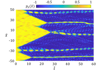
Figure 2: Single-trajectory 1D false vacuum simulation for the time evolution of $p_{z}$ at $\tau=1\times 10^{-5}$. The dimensionless length $\tilde{L}=100$ corresponds to a trap circumference $L=254\mathrm{\mu\mathrm{m}}$. Simulation parameters are: $\lambda=1.2$, $\widetilde{\nu}=7\times 10^{-3}$, $\widetilde{\omega}=50$, $\widetilde{\rho}=200$, number of modes $M=256$. The false vacuum ($p_{z}=1$) indicated by the yellow color decays, forming bubbles in the true vacua ($p_{z}=-1$) indicated by the blue regions.

From the simulations of our model at finite temperature, the thermal energy introduces extra thermal fluctuation into the system. The influence of the thermal fluctuation can result in an increase of tunneling events within the coupled BEC fields.

In addition, as shown in the single trajectory example in Figure 3, increasing the reduced temperature $\tau$ of the system enhances the interactions between the false vacua and the true vacua on long time scales. In the example of the low temperature dynamics shown in Figure 2, domain-wall and oscillon formation is minimized and the bubbles are well defined. This clear structure of the true vacuum is disturbed when the BEC is strongly thermalized as shown in Figure 3.

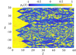
Figure 3: Single-trajectory 1D false vacuum simulation for the time evolution of $p_{z}$ at $\tau=3\times 10^{-4}$, all other parameters are as in Figure 2.

As can be seen in Figure 3, no stable domain walls or periodic oscillons are formed as the temperature increases, and no true vacuum bubbles survive on long time scales. As quantum tunneling is enhanced at higher temperatures, more bubbles are formed in the true vacua, but most of them are short-lived. Tunneling is accelerated at high temperatures, which leads to strong fluctuations between the true vacua and the false vacua, and many relatively unstable domain walls.

To quantify tunneling events, we can examine the average relative phase of the coupled fields along the axial coordinate, where

$$\langle\mathrm{cos}\phi_{a}\rangle =\frac{1}{\widetilde{L}}\intop^{\widetilde{L}}\mathrm{cos}\phi_{a}(\widetilde{x})d\widetilde{x}.$$ (57)

As illustrated in Figure 4, the relative average phase $\langle\mathrm{cos}\phi_{a}\rangle=1$ corresponds to an initial false vacuum. As the tunneling starts and the false vacuum decays to the true vacua, the average relative phase is expected to gradually decrease from $1$ to $-1$ in a complete transition. At very low temperatures, the presence of the true vacuum bubbles is noticeable with $\langle\mathrm{cos}\phi_{a}\rangle<-0.5$. However, at higher temperatures, the presence of the true vacuum bubbles is less noticeable due to the influence of the thermal fluctuations, and $\langle\mathrm{cos}\phi_{a}\rangle$ only goes to just below $0$. We define a threshold value $\langle\mathrm{cos}\phi_{a}\rangle=0.9$ as the initiation of the false vacuum tunneling event.

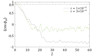
Figure 4: Time evolution of the corresponding average relative phase $\langle\mathrm{cos}\phi_{a}\rangle$ shown in Figure 2 (solid line) and Figure 3 (dash line), the horizontal dash-dot line $\langle\mathrm{cos}\phi_{a}\rangle=0.9$ indicates the threshold of the appearance of a true vacuum bubble.

Recalling that the tW method provides quantum estimation from a set of stochastic trajectories, hence to investigate the thermal effect on the tunneling rate at finite temperature conditions, we repeat the single trajectory simulation and determine the probability of bubble creation ($\langle\mathrm{cos}\phi_{a}\rangle\leq 0.9$) over time $P(\widetilde{t})$.

We then obtain the survival probability of the false vacuum $\mathcal{F}$ given that $\mathcal{F}=1-\int_{0}^{\widetilde{t}}P(\widetilde{t}^{\prime})d\widetilde{t}^{\prime}$. The tunneling rate $\Gamma$ for long time scales is calculated from a linear fit in log scale given that $\mathcal{F}=\mathrm{exp}(-\Gamma\widetilde{t})$ (Takagi, 2002). We performed simulations over a range of coupling strengths $\widetilde{\nu}$ and reduced temperatures $\tau$. Results are presented in Figure 5, 6 and 7. Previous work showed that larger couplings $\widetilde{\nu}$ extend the tunneling time (Fialko et al., 2015, 2017), which confirmed an expected slowing-down of quantum tunneling with dissipation (Caldeira and Leggett, 1981). To illustrate thermal effects, we compare the Bogoliubov thermal state results with the coherent state results which thermal noise is neglected. Although the coherent initial state is not a true Bogoliubov ground state, it has very similar behavior to the low temperature ground state. In the Wigner representation, the coherent initial state is represented by adding the quantum noise in each vacuum mode (37) to the classical false vacuum state. In dimensionless from, the coherent Wigner fields after the BEC is Rabi-rotated are $\widetilde{\psi}_{i=1,2}=\text{$\frac{\widetilde{\psi_{c}}}{\sqrt{2}}$}+\frac{1}{\sqrt{\widetilde{L}}}\sum\alpha_{\widetilde{k}}e^{i\widetilde{k}\widetilde{x}}$, where $\alpha_{\widetilde{k}}$ is an independent Gaussian random variable as already described in (40).

V.3 Thermally induced changes in decay rates

How does the finite initial temperature affect the decay of the false vacuum? From all three figures (Figure 5 to 7), the tunneling rates $\Gamma$ determined from both the coherent state and the thermal states at all tested temperatures $\tau$ show a power law dependence on $\widetilde{\nu}$. The gradients of $\log\Gamma$ for each effective modulation depth $\lambda$ are similar. If we compare the change of the tunneling rate $\Gamma$ at a fixed modulation depth $\lambda$, from each of Figure 5, 6 and 7, one can see that the rate of tunneling is increased as the temperature $\tau$ increases.

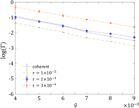
Figure 5: Dependence of the tunneling rate $\Gamma$ on the coupling $\widetilde{\nu}$ for different values of reduced temperature $\tau$ for $\lambda=1.2$. The error-bars show the estimated error of the linear least squares fitting in log scale.

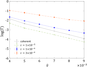
Figure 6: Tunneling rate $\Gamma$ for different values of reduced temperature $\tau$ for $\lambda=1.3$.

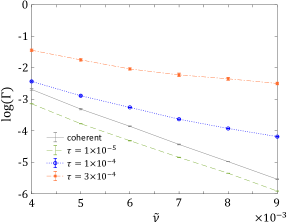
Figure 7: Tunneling rate $\Gamma$ for different values of reduced temperature $\tau$ for $\lambda=1.4$.

For the case of very low temperatures, $\tau=1\times 10^{-5}$, as the modulation depth $\lambda$ increases the tunneling rate is reduced more significantly than at higher temperatures. On the other hand, in the case of the highest reduced temperature studied ($\tau=3\times 10^{-4}$), this reduction of the tunneling rate due to an increase in $\lambda$ is less significant than at lower temperatures. The tunneling of the false vacuum is less restricted by $\lambda$ at higher temperatures.

This result suggests that at high temperatures, the effect of thermal fluctuations dominates the quantum decay of the false vacuum. For a fixed coupling strength $\widetilde{\nu}$, an increase of temperature increases the probability of penetrating the modulation depth barrier $\lambda$, and hence increases the formation rate of the true vacuum. The correlated ground state with $\tau=10^{-5}$ has a slightly lower tunneling rate than a coherent state, as it is stabilized by the Bogoliubov correlations. The qualitative effects of bubble nucleation and growth are similar in both cases.

V.4 Topological entropy results

The topological entropy allows us to quantify the phase disorder caused by the formation of true vacua and domain walls. Results for the topological entropy with $10^{4}$ distinct realizations are shown in Fig (8). Initially the coarse grained observational entropy is nearly zero, since all phase-space coordinates are in the metastable false vacuum. The observational entropy initially increases with time evolution, in contrast to the von Neumann quantum entropy which is constant with time. The entropy reaches a maximum as tunneling occurs, giving a nearly maximally disordered state with entropy $S<8\ln 3=8.79$, using $\ell=8,$ and $p=3.$ The entropy then reduces as the true vacua grow, reducing phase disorder.

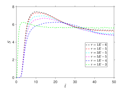
Figure 8: Evolution of the topological phase entropy function $S$ in early universe simulations using $10^{4}$ trajectories with varying order of magnitude, of reduced temperature $\tau$. Here the selected dimensionless parameters are $\widetilde{\nu}=7\times 10^{-3}$, $\lambda=1.2$, $\widetilde{\omega}=50$ and $\widetilde{\rho}=200$ with simulation parameters $\widetilde{L}=100$, space-phase bins $\ell=8$, $p=3$, with $N_{grid}=300$ and $8\times 10^{4}$ time steps.

The entropy function is shown to reach a maximum as a result of tunneling and after $\widetilde{t}\gtrsim 40$, it stabilizes to near $S\sim 8\ln 2$, as the false vacuum is eliminated. Between $\tau=10^{-6}$ and $\tau=10^{-4}$ shown by black and red curves, there is a decrease in the maximal entropy $S_{max}$ and lifetime of the peak. From $\tau=10^{-5}$ to $10^{-4}$, as $S_{max}$ decrease the lifetime of the peak increase. Beyond $\tau=10^{-4},$ the system thermalizes, as shown by the green curve.

At very low temperatures, the final state has almost no false vacuum. As a result, $S\leq 5.55$ as seen in the simulations of Figure 8. At higher temperatures the false vacuum never disappears completely, due to unstable domain wall formation, thus increasing the final state disorder. This is shown by the red and black scattered lines in Figure 8 and leads to the prediction of stable steady-state entropy values $S\sim 5.3$. The remaining disorder arises from the randomness due to the two topological phases of the true vacua and the remaining false vacuum domain wall or oscillating oscillons. The amount of disorder possible is limited by the spatial extent chosen for phase bins, and the number of samples used.

Figure 1 reveals true vacua states after a time $\widetilde{t}\gtrsim 3$, showing two different colors that depict the two different topological phases for the true vacuum. The true vacuum bubbles expand in space until they meet after a time $\widetilde{t}\gtrsim 15$ at $\widetilde{x}\approx-19$ and after a time $\widetilde{t}\gtrsim 24$ at $\widetilde{x}\approx 46$. The neighboring true vacuum regions with distinct topological phases are separated by a domain wall of false vacuum. On long time scales, Figure 1 clearly depicts the formation of an asymmetric structure of the topological phase in the true vacuum.

In Figure 9 we display the evolution of the entropy function $S(\widetilde{t})$ for different values of $\widetilde{\nu}$ using $10^{4}$ tW trajectories, and a comparison plot for the evolution of average relative phase $\langle\mathrm{cos}(\phi_{a})\rangle$ of the corresponding single trajectory examples. For larger couplings $\widetilde{\nu}$, the maximum entropy $S_{max}$ is reduced and the lifetime of the peak is extended. As the coupling $\widetilde{\nu}$ is increased, the tunneling initiation is generally delayed and the tunneling time is extended.

The single trajectory results presented in Figure 9 (b) are consistent with the expectation of a slowing-down of tunneling. We find similar behavior for the modulation depth $\lambda$ in the regime of metastability (for $\lambda>1$). In the case of large $\lambda$, bubble nucleation is delayed, with more results given in the Appendix.

The time evolution of the entropy function $S(\widetilde{t})$ for different numbers of spatial modes $M$ using $10^{4}$ trajectories is shown in Figure 10. The results are compared with the corresponding average relative phase $\langle\mathrm{cos}(\phi_{a})\rangle$ shown in Figure 10 (b). The evolution of $S(\widetilde{t})$ and $\langle\mathrm{cos}(\phi_{a})\rangle$ for higher spatial mode numbers are specified by black and red scattered lines in Figure 10. Systems with higher mode numbers have a more chaotic phase fluctuation, whereas the system with lower mode numbers specified by the blue dashed line show a smooth tunneling to the true vacuum.

The behavior is reflected in the entropy plots in Figure 10, where the narrow peaks of the entropy function for black and red scattered lines indicate a more chaotic phase ordering. On the other hand, the flattened peak of the entropy function for blue scattered line shows a relatively stable phase. In our simulations, the rapid transition to chaotic fluctuations at higher spatial modes can be minimized by increasing the characteristic frequency to $\widetilde{\omega}=200$ to achieve a stable tunneling to true vacuum. This behavior is caused by Floquet mode instabilities, and is an artifact of the microwave modulation frequency, as explained in greater detail in the Appendix.

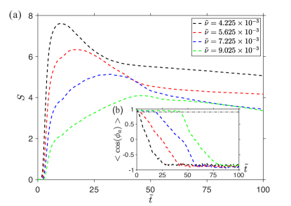
Figure 9: (a) Dependence of the entropy function $S(\widetilde{t})$ on coupling $\widetilde{\nu}$ calculated using $10^{4}$ trajectories with $\lambda=1.3$, $\widetilde{\omega}=50$, $\widetilde{\rho}=200$ and $\tau=10^{-5}$. (b) Average relative phase $\left\langle\cos(\phi_{a})\right\rangle=\frac{1}{\widetilde{L}}\intop_{0}^{\widetilde{L}}\cos\phi_{a}(\widetilde{x})d\widetilde{x}$ for single trajectory simulations for different values of $\widetilde{\nu}$. The horizontal dash-dot line $\left\langle\cos(\phi_{a})\right\rangle=0.9$ indicates the threshold of the appearance of a true vacuum bubble. The tunneling time is longer for larger couplings $\widetilde{\nu}$.

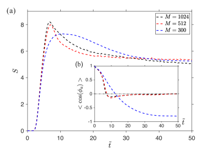
Figure 10: (a) Time evolution of the entropy $S(\widetilde{t})$ using $10^{4}$ trajectories for number of modes $M=300$, $512$ and $1024$. The dimensionless parameters chosen here are $\widetilde{\omega}=50$, $\tau=10^{-5}$, $\widetilde{\nu}=7\times 10^{-3}$, $\lambda=1.2$ and $\widetilde{\rho}=200$. (b) Time evolution of the average relative phase for different numbers of modes $M$. The horizontal dash-dotted line indicates a uniform random phase.

VI Conclusion

Prior to the present paper, the proposed experiment on the decay of a false vacuum had only been studied previously in the zero-temperature limit (Fialko et al., 2017; Opanchuk et al., 2013; Braden et al., 2018). As a result the effects of finite temperature thermal noise on vacuum tunneling and nucleation using BECs with two spin components were not understood. This mixture of two BEC spin components can be used as the relativistic analogous quantum field, where the relative phase of the two species corresponds to the metastable state (phase $\pi$) and stable state (phase zero) respectively. The components can be coupled via a microwave field, which creates an unstable vacuum.

To create a metastable vacuum from this unstable vacuum, one can make use of the classical concept of a modulated pendulum (Stephenson, 1908; Kapitza, 1965a, b; Stoker, 1950), where a modulated amplitude of microwave coupling allows one to engineer the metastable vacuum potential. We consider a symmetric intra-component case in this work for its simplicity. In previous work, we suggested the use of a pair of Zeeman states of ⁴¹K where $|1\rangle=|F=1,m_{F}=1\rangle$ and $|2\rangle=|F=1,m_{F}=0\rangle$ as the two spin states in the proposed BEC experiment. This Zeeman pair has a symmetrical intra-component Feshbach resonance where the inter-state scattering lengths between the two components are zero (Lysebo and Veseth, 2010).

We have shown in this paper that quantum vacuum nucleation is accelerated at finite temperature, although the bubbles formed of true vacua may be short-lived at high temperatures due to thermalization of the BEC. The formation of the true vacuum bubbles at finite temperature generally follows the expected behavior, apart from an accelerated tunneling rate. Clearly, lower temperatures move one further into the true quantum regime.

Our results also show that higher oscillator frequencies $\omega$ can remove short-wavelength instabilities, provided that there is a high-momentum cutoff present. This increases the feasibility of a false vacuum BEC experiment. The proposed table-top experiment using Zeeman states of ⁴¹K may help to test vacuum tunneling theory under real experimental conditions where thermal effects are unavoidable. This provides insight into early universe models with high temperatures, which is present in some early universe models (Zel’dovich et al., 1974).

Such an experiment can detect a unique topological feature of the scalar field vacuum. Unlike the von Neumann quantum entropy, which is time-invariant, the topological phase entropy is predicted to reach a maximum at the time when most tunneling occurs. Intriguingly, phase entropy can decrease with time, because the final vacuum state is more ordered than the state occurring while tunneling. This is a true topological feature of the present model, since the relative phase is only uniquely defined after a nonlocal unwrapping.

Such measurements may be useful in investigating proposals in which a discretely broken symmetry provides a model for particle-antiparticle symmetry. We find that domain wall formation is prevalent at high temperatures, in agreement with qualitative predictions (Zel’dovich et al., 1974; Kibble, 1980). However, at low temperatures domain walls are restricted to universe boundaries where they would be far removed from having a direct influence on CMB inhomogeneities, which was thought to be a possible problem with such theories.

Alternative implementations include a homogeneous, two dimensional simulation. This allows even more complex topological vacuum structures to form. Such experiments are realizable in micro-gravity with a shell geometry (Garraway and Perrin, 2016; Lundblad et al., 2019), for example in the NASA CAL space-station environment. There are many other possible approaches using different quantum technologies including superconducting circuits or discrete Bose-Hubbard lattices, which are not analyzed here.

Appendix: Modulational instabilities

Modulational instabilities can occur if the microwave modulation frequency $\omega$ is too low relative to the momentum cutoff. In such a case, the microwave modulation cannot be adiabatically eliminated, and parametric instabilities occur. The effect of such Floquet modes was studied by Braden et al. (Braden et al., 2018, 2019). In the work above, we have included a momentum cutoff to prevent this, as explained in the main text.

In this Appendix, we analyze the effects of modulational instabilities at finite temperatures with a higher momentum cutoff. The value of $\left\langle\cos\left(\phi_{a}\right)\right\rangle$ of the relative phase of such a system evolves to around $\sim 0$, indicating that the transition from the false vacuum to a true vacuum is inhibited, as the relative phase becomes completely randomized. This is studied numerically by choosing a smaller lattice spacing and lartger $M$, to resolve the high wave-number unstable modes.

The unstable modes occur in a narrow band centered at wave-numbers as derived in (Braden et al., 2018, 2019). The dimensionless critical unstable wavenumber is given by:

$$\widetilde{k}_{c}^{2} \approx \frac{1}{2\widetilde{\nu}}\left(\sqrt{1+\widetilde{\omega}^{2}\widetilde{\nu}}-1\right)-\sigma,$$ (58)

where $\sigma=\mathrm{cos}\phi_{a}=\pm 1$ is the relative phase of the fields.

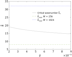
Figure 11: Critical wavenumber $\widetilde{k}_{c}$ and Nyquist wavenumber $\widetilde{k}_{nyq}=\pi/\Delta\widetilde{x}$ in the simulations for $\widetilde{\omega}=50$ at various values of $\widetilde{\nu}$ with fixed length $\widetilde{L}=100$. For $M=256$, $\widetilde{k}_{nyq}$ in the simulations are all below $\widetilde{k}_{c}$, hence the unstable modes are excluded. For $M=1024$, the unstable modes are included, as $\widetilde{k}_{nyq}>\widetilde{k}_{c}$.

Figure 11 shows the cutoff wave-numbers $\widetilde{k}_{nyq}$ in the simulations of previous sections (V.2) and (V.3) in comparison with the corresponding critical wave-numbers $\widetilde{k}_{c}$ at various values of $\widetilde{\nu}$. The Nyquist wavenumber determined by the lattice spacing $\Delta\widetilde{x}$, is $\widetilde{k}_{nyq}=\pi/\Delta\widetilde{x}$. The unstable wavenumber $\widetilde{k}_{c}$ is the wavenumber of the highest gain Floquet mode.

As shown in Figure 11, such effects are excluded in the $M=256$ simulations presented in sections (V.2) and (V.3) at all values of $\widetilde{\nu}$. Therefore, the short-wavelength fluctuations between the true vacua and the false vacua found at higher temperature (Figure 3) are purely due to the thermalization of the condensate. Thermal effects were excluded in earlier work (Braden et al., 2019). The dynamics at finite temperatures presented in Figure 3 shows similarities to the dynamics in the presence of the Floquet modes in (Braden et al., 2019). In the following we will investigate the combined effect of thermal fluctuations and Floquet instabilities on the dynamics, by setting $\widetilde{k}_{nyq}$ above the critical $\widetilde{k}_{c}$.

Figure 12 shows our results when both thermal effects and unstable Floquet modes are included. Here we reduce the lattice spacing $\Delta\widetilde{x}$ in the simulations by increasing the number of simulation modes to $M=1024$. This lattice spacing corresponds to a Nyquist wavenumber of $\widetilde{k}_{nyq}\approx 32.14$, well above the critical wavenumber $\widetilde{k}_{c}\approx 15.39$ for $\widetilde{\nu}=7\times 10^{-3}$.

The most significant effect of the unstable Floquet modes is that true vacua formed at finite temperature are gradually destroyed, and the system is eventually dominated by chaotic fluctuations. At a reduced temperature of $\tau=1\times 10^{-4}$, the presence of Floquet modes causes fluctuations with wavelengths shorter than the dominant thermal fluctuations.

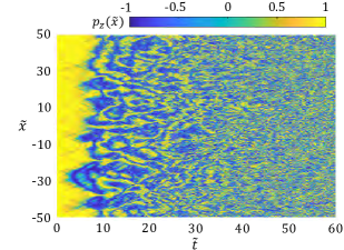
Figure 12: Single-trajectory 1D false vacuum simulation for the time evolution of $p_{z}$ at $\tau=1\times 10^{-4}$ with $M=1024$ to include the effect of Floquet modes. The modulation frequency is $\widetilde{\omega}=50$. Dimensionless parameters are $\tilde{L}=100$, $\lambda=1.2$, $\widetilde{\nu}=7\times 10^{-3}$, $\widetilde{\rho}=200$. Bubbles in the true vacua ($p_{z}=-1$) are short-lived and dominated by fluctuations at later time.

In Figure 2, 3 and 4 we show the effect of thermal fluctuations independently by setting $\widetilde{k}_{nyq}<\widetilde{k}_{c}$ to exclude Floquet modes. The true vacua in the absence of the Floquet modes have a metastable structure with average relative phase $\langle\mathrm{cos}\phi_{a}\rangle$ acquiring a non-zero constant value (Figure 4). However, this behavior is different in the presence of the Floquet modes, where the structure of the true vacua is short-lived.

In the example presented in Figure 12, most of the vacuum bubbles only survive over a time duration $5\apprle\widetilde{t}\lesssim 30$ (which corresponds to a real experimental time duration $\sim 20\mathrm{ms}$). At $\widetilde{t}\apprge 30$, one can expect the average relative phase $\langle\mathrm{cos}\phi_{a}\rangle$ to be around $\sim 0$ as the chaotic fluctuations dominate. This is confirmed by the averaged result using $8000$ trajectories shown in Figure 13.

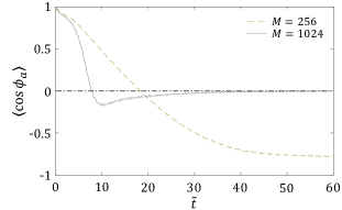
Figure 13: Time evolution of average relative phase $\langle\mathrm{cos}\phi_{a}\rangle$ using $8000$ trajectories for $M=256$ ($\widetilde{k}_{nyq}\approx 8.01<\widetilde{k}_{c}\approx 15.39$, Floquet modes excluded) and $M=1024$ ($\widetilde{k}_{nyq}\approx 32.14>\widetilde{k}_{c}\approx 15.39$, Floquet modes included). All other parameters are as in Figure 12. The errors in $\langle\mathrm{cos}\phi_{a}\rangle$ are less than $1\%$.

The modulation depth $\lambda$ is known to correspond to the strength of the unstable Floquet modes (Braden et al., 2018). In the absence of thermal effects, earlier studies (Braden et al., 2019) showed that increasing the modulation depth $\lambda$ can reduce the time-scale of the Floquet modes, and results in the stabilization of long-wavelength structure in the decay of false vacuum. This effectively delays the nucleation of the true vacuum bubbles. For systems at finite temperature where short-wavelength thermal fluctuations coexist with the true vacua, we found that this delay of bubble nucleation is valid. Figure 14 shows the examples on the effect of increasing $\lambda$ at a fixed reduced temperature $\tau=1\times 10^{-4}$.

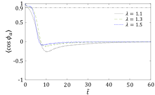
Figure 14: Time evolution of average relative phase $\langle\mathrm{cos}\phi_{a}\rangle$ using $8000$ trajectories for $\lambda=1.1$ (solid line), $\lambda=1.3$ (dash line), and $\lambda=1.5$ (dot line). Floquet modes are included by setting number of modes $M=1024$ ($\widetilde{k}_{nyq}\approx 32.14>\widetilde{k}_{c}\approx 15.39$). Reduced temperature $\tau=1\times 10^{-4}$, other dimensionless parameters $\widetilde{L}=100$, $\widetilde{\omega}=50$, $\widetilde{\nu}=7\times 10^{-3}$, $\widetilde{\rho}=200$. The errors in $\langle\mathrm{cos}\phi_{a}\rangle$ are less than $1\%$.

At time $\widetilde{t}\lesssim 10$, our results show that the systems with larger $\lambda$ ($\lambda=1.3,1.5$) break through the threshold value of the tunneling initiation $\langle\mathrm{cos}\phi_{a}\rangle=0.9$ later than the $\lambda=1.1$ system, indicating a delay of the bubble nucleation. In the presence of Floquet instabilities, increasing $\lambda$ results in a significant reduction of the average relative phase. The peak value of $|\langle\mathrm{cos}\phi_{a}\rangle|$ drops from $\sim 0.35$ to $\sim 0.1$ as $\lambda$ is increased from $1.1$ to $1.5$. For decay at finite temperature, we have shown in the main text Figure 4 that this phase signal is also weakened by the influence of thermal fluctuations in the absence of the Floquet instabilities.

Increasing $\lambda$ in the presence of Floquet modes further reduces the phase signal, which increases the difficulty of measuring true vacua in an experiment. Therefore, it is expected that true vacuum bubbles are destroyed by Floquet instabilities regardless of $\lambda$. At time $\widetilde{t}\gtrsim 10$ in Figure 14, the average relative phase of all three systems reaches $\sim 0$ eventually. The true vacuum bubbles in the system with the lowest $\lambda$ survive longer due to their larger sizes. In the case where Floquet instabilities are not negligible, the tuning of the modulation depth $\lambda$ plays a role in the balance between time duration and strength of true vacua signals.

In order to remove the unstable Floquet modes from the system, one can increase the oscillation frequency $\widetilde{\omega}$ to shift $\widetilde{k}_{c}$ to higher wave-numbers above the increased momentum cutoff used in this Appendix. Figure 15 illustrates the simulated dynamics of the false vacuum at a fixed temperature $\tau=1\times 10^{-4}$ , and increasing $\widetilde{\omega}$.

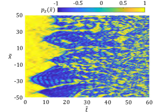
Figure 15: Single-trajectory simulation for $p_{z}$ at $\tau=1\times 10^{-4}$ with $M=1024$. The modulation frequency is $\widetilde{\omega}=150$. Floquet modes are included: $\widetilde{k}_{nyq}\approx 32.1>\widetilde{k}_{c}\approx 28.8$. Dimensionless parameters $\tilde{L}=100$, $\lambda=1.2$, $\widetilde{\nu}=7\times 10^{-3}$, $\widetilde{\rho}=200$. Comparing to Figure 12, the true vacuum ($p_{z}=-1$) is relatively long-lived and stable .

In Figure 15, the results show that the stabilization of true vacua is sensitive to an increase of $\widetilde{\omega}$. Both the lifetime and the phase signal of the true vacua are enhanced. In comparison with Figure 12 ($\widetilde{\omega}=50$ at $\tau=1\times 10^{-4}$), increasing $\widetilde{\omega}$ to $150$ (Figure 15) extends the sizes of the true vacuum bubbles and the chaotic fluctuations are suppressed in the true vacua. The survival time of the true vacuum bubbles before domination by fluctuations is also improved slightly when $\widetilde{\omega}$ is increased, from roughly $\widetilde{t}\lesssim 30$ for $\widetilde{\omega}=50$ to $\widetilde{t}\apprle 40$ for $\widetilde{\omega}=150$.

As mentioned, the simulated system with $\widetilde{\omega}=50$ in Figure 12 includes the Floquet modes by setting $\widetilde{k}_{nyq}\approx 32.14$ well above the critical wavenumber $\widetilde{k}_{c}\approx 15.39$; while for the system with $\widetilde{\omega}=150$, the Floquet modes are partially removed as the critical wavenumber is increased to $\widetilde{k}_{c}\approx 28.79$. This partial removal of the Floquet modes reduces the chaotic fluctuations and results in the partial stabilization of true vacua.

If we further increase the modulation frequency to $\widetilde{\omega}=200$, the critical wavenumber is shifted to $\widetilde{k}_{c}\approx 33.57$ which is slightly higher than $\widetilde{k}_{nyq}$. In this case, the Floquet modes are almost completely excluded. Figure 16 shows that in the dynamics of the false vacuum with $\widetilde{\omega}=200$, one can see that the size of the true vacuum bubbles are extended, and a break-down of the vacuum bubbles is not observed in the simulation.

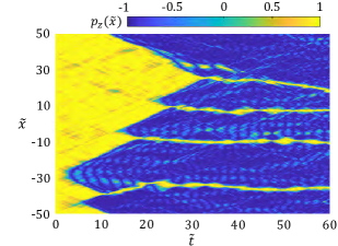
Figure 16: Single-trajectory simulation for the time evolution of $p_{z}$ with an increased frequency $\widetilde{\omega}=200$ to remove the Floquet modes ($\widetilde{k}_{nyq}\approx 32.14<\widetilde{k}_{c}\approx 33.57$). Other parameters are as in Figure 15.

Increasing $\widetilde{\omega}$ to suppress the chaotic fluctuations induced by the presence of the Floquet instabilities has a significant effect on the stabilization of true vacua. Figure 17 shows that the suppression of the chaotic fluctuations enhances the average relative phase $\langle\mathrm{cos}\phi_{a}\rangle$. The relative phase can reach $\langle\mathrm{cos}\phi_{a}\rangle\approx-0.75$ even at the high reduced temperature $\tau=1\times 10^{-4}$, which is comparable to a measurement at a lower temperature $\tau=1\times 10^{-5}$ ($\langle\mathrm{cos}\phi_{a}\rangle\approx-0.8\sim-0.9$, in Figure 4).

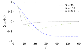
Figure 17: Time evolution of $\langle\mathrm{cos}\phi_{a}\rangle$ using $8000$ trajectories for $\widetilde{\omega}=50$ (solid line), $150$ (dash line) and $200$ (dot line), all other parameters are as in Figure 15. The errors in $\langle\mathrm{cos}\phi_{a}\rangle$ are less than $1\%$.

In summary, bubble nucleation and break-down are delayed by increasing $\widetilde{\omega}$ to remove the Floquet modes. From the averaged results using $8000$ trajectories, true vacua reach their peak size at a time $\widetilde{t}\approx 10$ for $\widetilde{\omega}=50$ and $\widetilde{t}\approx 20$ for $\widetilde{\omega}=150$, and are later destroyed by chaotic fluctuations due to Floquet modes (i.e. $\langle\mathrm{cos}\phi_{a}\rangle\approx 0$). For $\widetilde{\omega}=200$, the time of the peak relative phase is delayed to $\widetilde{t}\approx 35$ and $\langle\mathrm{cos}\phi_{a}\rangle$ remains $\sim-0.8$ over the remaining simulation time duration. The high dimensionless frequency $\widetilde{\omega}=200$ in the simulations corresponds to an oscillation frequency $\omega=2\pi\times 38.24\mathrm{kHz}$, which is achievable in current experiments. We emphasize that this still requires an overall momentum cutoff, although at a higher wavenumber.

References

- Coleman (1977) S. Coleman, Phys. Rev. D 15, 2929 (1977).
- Callan and Coleman (1977) C. G. Callan and S. Coleman, Phys. Rev. D 16, 1762 (1977).
- Guo et al. (2020) Y. Guo, R. Dubessy, M. G. deHerve, A. Kumar, T. Badr, A. Perrin, L. Longchambon, and H. Perrin, Phys. Rev. Lett. 124, 025301 (2020).
- Hopkins et al. (2004) A. Hopkins, B. Lev, and H. Mabuchi, Phys. Rev. A 70, 053616 (2004).
- Bell et al. (2016) T. A. Bell, J. A. P. Glidden, L. Humbert, M. W. J. Bromley, S. A. Haine, M. J. Davis, T. W. Neely, M. A. Baker, and H. Rubinsztein-Dunlop, New Journal of Physics 18, 035003 (2016).
- Sakharov (1991) A. D. Sakharov, Soviet Physics Uspekhi 34, 392 (1991).
- Zel’dovich et al. (1974) Y. B. Zel’dovich, I. Y. Kobzarev, and L. B. Okun, Zh. Eksp. Teor. Fiz. 67, 3 (1974).
- Kibble (1980) T. W. B. Kibble, Physics Reports 67, 183 (1980).
- Abel and Spannowsky (2020) S. Abel and M. Spannowsky, “Observing the fate of the false vacuum with a quantum laboratory,” (2020), arXiv:2006.06003 [hep-th] .
- Drummond and Hardman (1993) P. D. Drummond and A. D. Hardman, EPL (Europhysics Letters) 21, 279 (1993).
- Steel et al. (1998) M. J. Steel, M. K. Olsen, L. I. Plimak, P. D. Drummond, S. M. Tan, M. J. Collett, D. F. Walls, and R. Graham, Phys. Rev. A 58, 4824 (1998).
- Kinsler and Drummond (1991) P. Kinsler and P. D. Drummond, Phys. Rev. A 43, 6194 (1991).
- Linde (1982) A. D. Linde, Phys. Lett. B 108, 389 (1982).
- Opanchuk et al. (2013) B. Opanchuk, R. Polkinghorne, O. Fialko, J. Brand, and P. D. Drummond, Annalen der Physik 525, 866 (2013).
- Fialko et al. (2015) O. Fialko, B. Opanchuk, A. I. Sidorov, P. D. Drummond, and J. Brand, EPL (Europhysics Letters) 110, 56001 (2015).
- Fialko et al. (2017) O. Fialko, B. Opanchuk, A. I. Sidorov, P. D. Drummond, and J. Brand, J. Phys. B: At. Mol. Opt. Phys. 50, 024003 (2017).
- Billam et al. (2019) T. P. Billam, R. Gregory, F. Michel, and I. G. Moss, Phys. Rev. D 100, 065016 (2019).
- Bogolubov (1947) N. Bogolubov, J. Phys.(USSR) 11, 23 (1947), [Izv. Akad. Nauk Ser. Fiz.11,77(1947)].
- Ng et al. (2018) K. L. Ng, R. Polkinghorne, B. Opanchuk, and P. D. Drummond, J. Phys. A: Math. Theor. 52, 035302 (2018).
- Corney et al. (2006) J. F. Corney, P. D. Drummond, J. Heersink, V. Josse, G. Leuchs, and U. L. Andersen, Phys. Rev. Lett. 97, 023606 (2006).
- Corney et al. (2008) J. F. Corney, J. Heersink, R. Dong, V. Josse, P. D. Drummond, G. Leuchs, and U. L. Andersen, Phys. Rev. A 78, 023831 (2008).
- Egorov et al. (2011) M. Egorov, R. P. Anderson, V. Ivannikov, B. Opanchuk, P. D. Drummond, B. V. Hall, and A. I. Sidorov, Phys. Rev. A 84, 021605(R) (2011).
- Drummond and Opanchuk (2017) P. D. Drummond and B. Opanchuk, Phys. Rev. A 96, 043616 (2017).
- Opanchuk et al. (2019) B. Opanchuk, L. Rosales-Zárate, R. Y. Teh, B. J. Dalton, A. Sidorov, P. D. Drummond, and M. D. Reid, Phys. Rev. A 100, 060102(R) (2019).
- Guralnik et al. (1964) G. S. Guralnik, C. R. Hagen, and T. W. B. Kibble, Phys. Rev. Lett. 13, 585 (1964).
- Higgs (1964) P. W. Higgs, Phys. Rev. Lett. 13, 508 (1964).
- Englert and Brout (1964) F. Englert and R. Brout, Phys. Rev. Lett. 13, 321 (1964).
- Yurovsky et al. (2017) V. A. Yurovsky, B. A. Malomed, R. G. Hulet, and M. Olshanii, Phys. Rev. Lett. 119, 220401 (2017).
- Guth (1981) A. H. Guth, Phys. Rev. D 23, 347 (1981).
- Musoke et al. (2020) N. Musoke, S. Hotchkiss, and R. Easther, Phys. Rev. Lett. 124, 061301 (2020).
- Mukhanov et al. (1992) V. Mukhanov, H. Feldman, and R. Brandenberger, Physics Reports 215, 203 (1992).
- Drummond and Kinsler (1989) P. D. Drummond and P. Kinsler, Phys. Rev. A 40, 4813 (1989).
- Sinatra et al. (2002) A. Sinatra, C. Lobo, and Y. Castin, J. Phys. B: At. Mol. Opt. Phys. 35, 3599 (2002).
- Deuar and Drummond (2007) P. Deuar and P. D. Drummond, Phys. Rev. Lett. 98, 120402 (2007).
- Yurke and Stoler (1986) B. Yurke and D. Stoler, Phys. Rev. Lett. 57, 13 (1986).
- Budroni et al. (2015) C. Budroni, G. Vitagliano, G. Colangelo, R. J. Sewell, O. Gühne, G. Tóth, and M. W. Mitchell, Phys. Rev. Lett. 115, 200403 (2015).
- Kovachy et al. (2015) T. Kovachy, P. Asenbaum, C. Overstreet, C. A. Donnelly, S. M. Dickerson, A. Sugarbaker, J. M. Hogan, and M. A. Kasevich, Nature 528, 530 (2015).
- Opanchuk et al. (2016) B. Opanchuk, L. Rosales-Zárate, R. Y. Teh, and M. D. Reid, Phys. Rev. A 94, 062125 (2016).
- Rosales-Zárate et al. (2018) L. Rosales-Zárate, B. Opanchuk, Q. Y. He, and M. D. Reid, Phys. Rev. A 97, 042114 (2018).
- Thenabadu et al. (2020) M. Thenabadu, G.-L. Cheng, T. L. H. Pham, L. V. Drummond, L. Rosales-Zárate, and M. D. Reid, Phys. Rev. A 102, 022202 (2020).
- Opanchuk and Drummond (2017) B. Opanchuk and P. D. Drummond, Phys. Rev. A 96 (2017).
- Rosenbluh and Shelby (1991) M. Rosenbluh and R. M. Shelby, Phys. Rev. Lett. 66, 153 (1991).
- Ng et al. (2019) K. L. Ng, B. Opanchuk, M. D. Reid, and P. D. Drummond, Phys. Rev. Lett. 122, 203604 (2019).
- Marchukov et al. (2020) O. V. Marchukov, B. A. Malomed, V. Dunjko, J. Ruhl, M. Olshanii, R. G. Hulet, and V. A. Yurovsky, Phys. Rev. Lett. 125, 050405 (2020).
- Kupiszewska and Rzazewski (1990) D. Kupiszewska and K. Rzazewski, Phys. Rev. A 42, 6869 (1990).
- Kinsler et al. (1993) P. Kinsler, M. Fernée, and P. D. Drummond, Phys. Rev. A 48, 3310 (1993).
- Leggett (2001) A. J. Leggett, Rev. Mod. Phys. 73, 307 (2001).
- Opanchuk and Drummond (2013) B. Opanchuk and P. D. Drummond, J. Math. Phys. 54, 042107 (2013).
- Deuar et al. (2009) P. Deuar, A. G. Sykes, D. M. Gangardt, M. J. Davis, P. D. Drummond, and K. V. Kheruntsyan, Phys. Rev. A 79, 043619 (2009).
- Olshanii (1998) M. Olshanii, Phys. Rev. Lett. 81, 938 (1998).
- Kheruntsyan et al. (2005) K. V. Kheruntsyan, D. M. Gangardt, P. D. Drummond, and G. V. Shlyapnikov, Phys. Rev. A 71, 053615 (2005).
- Bouchoule et al. (2012) I. Bouchoule, M. Arzamasovs, K. V. Kheruntsyan, and D. M. Gangardt, Phys. Rev. A 86, 033626 (2012).
- Stephenson (1908) A. Stephenson, The London, Edinburgh, and Dublin Philosophical Magazine and Journal of Science 15, 233 (1908).
- Stoker (1950) J. J. Stoker, Nonlinear vibrations in mechanical and electrical systems (Interscience Publishers, New York, 1950).
- Kapitza (1965a) P. L. Kapitza, in Collected Papers of P.L. Kapitza, edited by D. T. HAAR (Pergamon, 1965) pp. 714 – 725.
- Kapitza (1965b) P. L. Kapitza, in Collected Papers of P.L. Kapitza, edited by D. T. HAAR (Pergamon, 1965) pp. 726 – 737.
- Ibrahim (2006) R. A. Ibrahim, Journal of Vibration and Control 12, 1093 (2006).
- Freedhoff and Chen (1990) H. Freedhoff and Z. Chen, Phys. Rev. A 41, 6013 (1990).
- Zhu et al. (1990) Y. Zhu, Q. Wu, A. Lezama, D. J. Gauthier, and T. W. Mossberg, Phys. Rev. A 41, 6574 (1990).
- Braden et al. (2018) J. Braden, M. C. Johnson, H. V. Peiris, and S. Weinfurtner, Journal of High Energy Physics 2018, 14 (2018).
- Braden et al. (2019) J. Braden, M. C. Johnson, H. V. Peiris, A. Pontzen, and S. Weinfurtner, Journal of High Energy Physics 2019, 174 (2019).
- Cornell and Wieman (2002) E. A. Cornell and C. E. Wieman, Rev. Mod. Phys. 74, 875 (2002).
- Ketterle and Van Druten (1996) W. Ketterle and N. J. Van Druten, Advances in Atomic, Molecular, and Optical Physics 37, 181 (1996).
- Bradley et al. (1997) C. C. Bradley, C. A. Sackett, and R. G. Hulet, Phys. Rev. Lett. 78, 985 (1997).
- Drummond and Corney (1999) P. D. Drummond and J. F. Corney, Phys. Rev. A 60, R2661 (1999).
- Glauber (1963) R. J. Glauber, Phys. Rev. 131, 2766 (1963).
- Louisell (1973) W. H. Louisell, Quantum statistical properties of radiation, Wiley series in pure and applied optics (Wiley, New York, 1973).
- Drummond and Hillery (2014) P. D. Drummond and M. Hillery, The Quantum Theory of Nonlinear Optics (Cambridge University Press, 2014).
- Gardiner (1997) C. W. Gardiner, Phys. Rev. A 56, 1414 (1997).
- Boccato et al. (2019) C. Boccato, C. Brennecke, S. Cenatiempo, and B. Schlein, Acta Math. 222, 219 (2019).
- Fetter (1972) A. L. Fetter, Annals of Physics 70, 67 (1972).
- Lewenstein and You (1996) M. Lewenstein and L. You, Phys. Rev. Lett. 77, 3489 (1996).
- Kheruntsyan et al. (2003) K. V. Kheruntsyan, D. M. Gangardt, P. D. Drummond, and G. V. Shlyapnikov, Phys. Rev. Lett. 91, 040403 (2003).
- Wigner (1932) E. P. Wigner, Phys. Rev. 40, 749 (1932).
- Norrie et al. (2006) A. A. Norrie, R. J. Ballagh, and C. W. Gardiner, Phys. Rev. A 73, 043617 (2006).
- Drummond et al. (1993) P. D. Drummond, R. M. Shelby, S. R. Friberg, and Y. Yamamoto, Nature 365, 307 (1993).
- Ruostekoski and Isella (2005) J. Ruostekoski and L. Isella, Phys. Rev. Lett. 95, 110403 (2005).
- Isella and Ruostekoski (2006) L. Isella and J. Ruostekoski, Phys. Rev. A 74, 063625 (2006).
- Jaynes (1965) E. T. Jaynes, Am. J. Phys. 33, 391 (1965).
- Wehrl (1978) A. Wehrl, Rev. Mod. Phys. 50, 221 (1978).
- Swendsen (2011) R. H. Swendsen, Am. J. Phys. 79, 342 (2011).
- Balibrea (2016) F. Balibrea, Journal of Modern Physics 07, 219 (2016).
- Goldstein et al. (2019) S. Goldstein, D. Huse, J. L. Lebowitz, and P. Sartori, in Stochastic Dynamics Out of Equilibrium, Springer Proceedings in Mathematics and Statistics, Vol. 282, edited by G. Giacomin, S. Olla, E. Saada, H. Spohn, and G. Stoltz (Springer International Publishing, Cham, 2019) pp. 581–596.
- Wehrl (1979) A. Wehrl, Rep. Math. Phys. 16, 353 (1979).
- Husimi (1940) K. Husimi, Proc. Phys. Math. Soc. Jpn. 22, 264 (1940).
- Drummond and Reid (2020) P. D. Drummond and M. D. Reid, Phys. Rev. Research 2, 033266 (2020).
- Reid (2017) M. D. Reid, J. Phys. A: Math. Theor. 50, 41LT01 (2017).
- Cahill and Glauber (1969) K. E. Cahill and R. J. Glauber, Phys. Rev. 177 (1969).
- Šafránek et al. (2020) D. Šafránek, A. Aguirre, J. Schindler, and J. M. Deutsch, “A brief introduction to observational entropy,” (2020), arXiv:2008.04409 [quant-ph] .
- Itoh (1982) K. Itoh, Appl. Opt. 21, 2470 (1982).
- Kiesewetter et al. (2016) S. Kiesewetter, R. Polkinghorne, B. Opanchuk, and P. D. Drummond, SoftwareX 5, 12 (2016).
- Takagi (2002) S. Takagi, Macroscopic Quantum Tunneling (Cambridge University Press, 2002).
- Caldeira and Leggett (1981) A. O. Caldeira and A. J. Leggett, Phys. Rev. Lett. 46, 211 (1981).
- Lysebo and Veseth (2010) M. Lysebo and L. Veseth, Phys. Rev. A 81, 032702 (2010).
- Garraway and Perrin (2016) B. M. Garraway and H. Perrin, J. Phys. B: At. Mol. Opt. Phys. 49, 172001 (2016).
- Lundblad et al. (2019) N. Lundblad, R. A. Carollo, C. Lannert, M. J. Gold, X. Jiang, D. Paseltiner, N. Sergay, and D. C. Aveline, npj Microgravity 5, 30 (2019).