iint TXFiint

Sleeping beasts: strong toroidal magnetic field in quiescent magnetars explains their large pulsed fraction

Magnetars are neutron stars (NSs) with extreme magnetic fields¹ of strength $5\times 10^{13}\mathrel{-}10^{15}$ G. They exhibit transient, highly energetic events, such as short X-ray flashes, bursts and giant flares, all of which are powered by their enormous magnetic energy ². Quiescent magnetars have X-ray luminosities between $10^{29}$ and $10^{35}$ erg/s, and are further classified as either persistent or transient magnetars. Their X-ray emission is modulated with the rotational period of the NS, with a typical relative amplitude (so-called pulsed fraction) between 10-58 per cent, implying that the surface temperature is significantly non-uniform despite the high thermal conductivity of the star’s crust. Here, we present the first 3D magneto-thermal MHD simulations of magnetars with strong toroidal magnetic fields. We show that these models, combined with ray propagation in curved space-time, accurately describe the light-curves of most transient magnetars in quiescence and allow us to further constrain their rotational orientation. We find that the presence of a strong toroidal magnetic field explains the observed asymmetry in the surface temperature, and is the main cause of the strong modulation of thermal X-ray emission in quiescence.

Soft X-ray emission from magnetars in quiescence originates from their surface, either at the top of their solid outer crust or their atmosphere. Magnetic fields deeper in the crust control the surface temperature distribution and consequently the X-ray emission. The magnetic field provides heating through its Ohmic decay, and also governs how this heat flows through the crust, by inhibiting diffusion perpendicular to magnetic field lines. Regions of open field lines cool rapidly, while heat remains trapped in regions of closed field lines ³. The field is generated by dynamo action during the proto-NS phase, and is expected to have both poloidal and toroidal components ⁴, ⁵, although the energy of the toroidal component could be ten times larger ⁶. Only the poloidal field can be measured directly, via the neutron star spin-down ⁷, but there is also observational evidence of a strong toroidal field. The toroidal component is responsible for magnetospheric twisting and, therefore, the transient behaviour of magnetars ⁸. The X-ray spectra of many magnetars are best described if a large toroidal magnetic field is assumed ⁹, ¹⁰.

When interpreting X-ray observations, the surface thermal pattern resulting from magneto-thermal evolution is approximated empirically as a collection of circular regions with different temperatures ¹¹. Originally, these regions were placed at the magnetic poles of an assumed dipolar field ¹², but such a configuration cannot produce a large pulsed fraction ¹³. Therefore modern interpretations allow for regions that do not coincide with the magnetic poles, and have varying sizes and temperatures ¹¹. To explain the formation, location and shape of these hot surface regions requires a detailed three-dimensional model of the temperature and magnetic field in the crust.

Here we investigate for the first time the formation and evolution of hotter and colder regions at the surface of a quiescent magnetar, using three-dimensional magnetohydrodynamic (MHD) simulations in a spherical shell performed with a modified version of the PARODY code ¹⁴ (see also Methods Section 1). We simulate the magneto-thermal evolution for two field configurations that have strong toroidal fields containing 90% of the total magnetic energy: in model A the poloidal and toroidal components are aligned, and in model B the toroidal magnetic field is inclined by $45^{\circ}$ with respect to the poloidal dipole. The initial dipole magnetic field is $1.3\times 10^{13}$ G; the maximum values of magnetic field in the crust at the beginning of the simulations are $1.2\times 10^{15}$ G. Figure 1 shows the surface temperature distribution for these models after about 20 Kyr of evolution. The isothermal, purely magnetic properties of these models have previously been studied in detail¹⁵. The filamentary pattern of hot and cold regions visible in Figure 1 reflects the magnetic field structure arising from an instability of the toroidal field ¹⁶. Both models exhibit north-south asymmetry: model A has a hot zone that wraps around the dipole axis, whereas model B has a single hot spot. The size of these hot zones are consistent with observations of quiescent magnetars by X-ray spectroscopy.

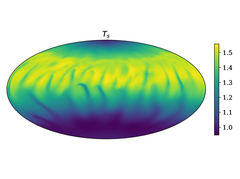
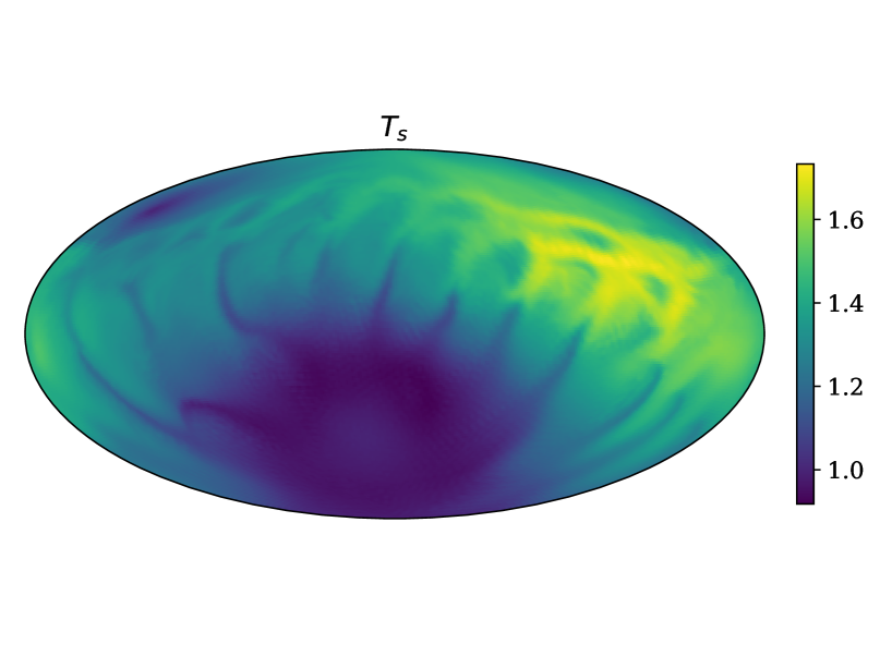
Fig. 1: Thermal maps obtained in 3D magneto-thermal simulations. Left panel: model A for NS with aligned poloidal and toroidal magnetic fields, age 18 Kyr. Right panel: model B for NS with poloidal and toroidal magnetic fields inclined by angle of $45^{\circ}$, age 24 Kyr. The surface temperatures are in units of MK.

We further compute the light-curves produced by each of these models (see Methods Section 2 for details) taking into account relativistic effects. We assume that the NS has radius $R=12$ km and mass $M=1.4~{}M_{\odot}$. Because magnetars rotate relatively slowly, we use approximations for ray propagation in the Schwarzschild metric. We find that models A and B have soft X-ray luminosities of $0.8-2\times 10^{32}$ erg/s and pulsed fraction ranges from 16 to 53 per cent, which is consistent with observations of transient magnetars. By contrast, models that have weak toroidal magnetic fields have a temperature distribution that is very symmetric with respect to the magnetic equator ¹², and typically have a maximum pulsed fraction of $\approx 10$%. For a given surface temperature distribution, the light-curve depends on three angular parameters: $\kappa$ the angle between the dipole axis and the rotation axis, $i$ the angle between the observer’s line of sight and the rotation axis, and $\Delta\Phi$ the phase shift. We fit our light-curves to the folded soft X-ray emission of seven transient magnetars in quiescence with $L_{X}\lesssim 10^{33}$ erg/s. The details of the observational reduction and the fitting procedure can be found in Methods Sections 3 and 4 respectively. Briefly, we analyse old observations of magnetars in quiescence and produce period-folded light-curves in the soft X-ray range 0.3-2 KeV. Our fits are weakly sensitive to the assumed radius and mass of the NS.

Source name	$\kappa$	$i$	$\Delta\Phi$	Age	Model	$\chi^{2}/$d.o.f.	$L^{0.3-2~{}\mathrm{KeV}}_{x}$
	$(^{\circ})$	$(^{\circ})$	$(^{\circ})$	(Kyr)			$10^{32}$ erg/s
SGR 0418+5729	$230\pm 26$	$274\pm 22$	$217\pm 9$	24.0	B	6.0/13	0.0077
1E 1547.0-5408	$106\pm 8$	$27\pm 3$	$175\pm 5$	17.7	A	9.3/13	19
CXOU J164710.0-455216	$206\pm 33$	$69\pm 22$	$32\pm 6$	31.7	B	24.0/13	5.5
XTE J1810–197	$153\pm 3$	$33\pm 6$	$161\pm 5$	18	A	13.8/13	5.8
Swift J1822.3-1606	$193\pm 12$	$284\pm 13$	$217\pm 6$	13.6	B	18.3/13	0.81
SGR 0501+4516	104.3	74.8	174.7	6.5	A	76.3/13	$3.10$
3XMM J185246.6+003317	208.3	69.2	36.7	31.7	B	40.6/13	$\sim 20.00$

Table 1: Best-fit parameters for the folded X-ray light-curves of seven magnetars. Error bars are $95\%$ confidence intervals. In the case of 3XMM J185246.6+003317 the column density $N_{\text{H}}$ is unknown, so the X-ray luminosity is indicative of typical $N_{\text{H}}$.

The parameters that produce the best fit in each case are summarised in Table 1. For the four magnetars SGR 0418+5729, 1E 1547.0-5408, XTE J1810-197 and Swift J1822.3-1606 we obtain perfectly acceptable fits; see examples in Figure 2. In the case of CXOU J164710.0-455216 our fit is marginally acceptable. The temperature distribution produced as a result of magneto-thermal evolution in the crust describes extremely well the soft X-ray emission of these objects in quiescence. The asymmetries previously found in the light-curve are naturally explained by the presence of large toroidal magnetic fields, which causes strong currents to accumulate in one of the hemispheres ¹⁷. We briefly discuss two cases that are described less successfully by our model in Methods Section 5. Our estimate for the angle $\kappa=106^{\circ}$ for 1E 1547.0-5408 is somewhat different from the value inferred from radio observations¹⁸ $\kappa=160^{\circ}$. This difference could be caused by a non-dipolar magnetic field with complicated magnetic structure. Alternatively, fitting against model B at the age $24$ Kyr gives a very different angle, $\kappa\approx 16^{\circ}$ ($\chi^{2}=14$), which is a nearly aligned rotator and agrees better with the radio data.

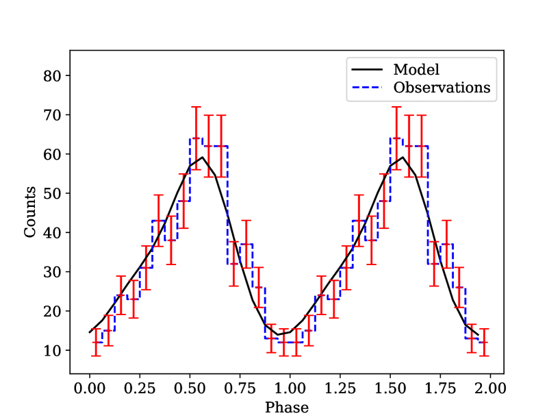
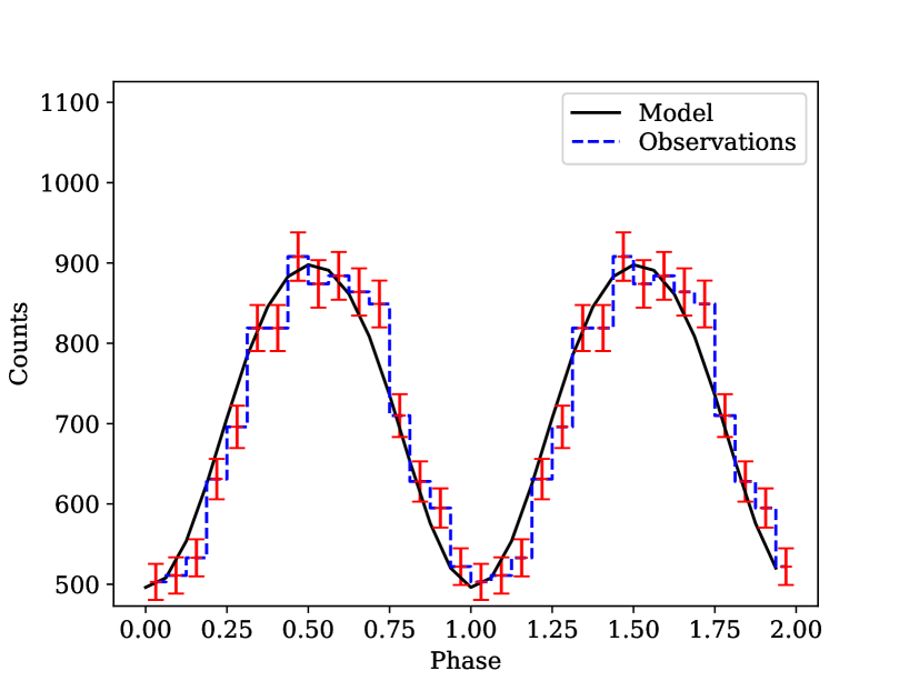
Fig. 2: Folded soft X-ray light-curve (300-2000 eV) for magnetars. Left panel: SGR 0418+5729, right panel: 1E 1547.0-5408. The dashed blue lines and red error bars are observations and $1\sigma$ confidence intervals. The solid black lines are the theoretical light-curve for the most favourable orientation.

Our model only describes the magnetic field evolution in the NS crust. Further work is needed to better understand the magnetic field evolution in the NS core, where ambipolar diffusion might play an important role¹⁹, particularly in very young NSs. Whether field evolution in the core is significant for quiescent magnetars is unknown.

The toroidal magnetic field, which is the main source of the magnetospheric twist, could also cause crust yielding. We have shown that the same toroidal magnetic field can naturally explain the X-ray emission of quiescent magnetars. Therefore, possibly the main difference between a magnetar and a strongly magnetised neutron star which shows no magnetar-like behaviour is the strength of the toroidal magnetic field in the crust. With the revolutionary insight obtained by the NICER telescope for recycled pulsars ²⁰, ²¹, it is becoming increasingly clear that the magnetic field structure of NSs is complicated, so it is extremely important to explore the process of magnetic field evolution and formation for NSs.

In summary, our results provide strong support that an intense crustal toroidal field is an essential ingredient, not only for the magnetospheric behaviour, but also the thermal radiation originating from the crust. As well as providing heat through Ohmic decay, it is also responsible for the formation of thermal spots. Our simulation results not only produce qualitative agreement with the observational data, but also provide constraints on the strength and geometry of magnetar magnetic fields.

Methods

1 MHD and Thermal simulations

We integrate the two coupled equations describing magnetic induction and heat transfer within the NS crust:

$$\frac{\partial\vec{B}}{\partial t} = -c\nabla\times\left\{\frac{1}{4\pi en_{e}}(\nabla\times\vec{B})\times\vec{B}+\frac{c}{4\pi\sigma}\nabla\times\vec{B}-\frac{1}{e}S_{e}\nabla T\right\}\,,$$ (1)

$$C_{V}\frac{\partial T}{\partial t} = \nabla\cdot(k\cdot\nabla T)+\frac{|\nabla\times\vec{B}|^{2}c^{2}}{16\pi^{2}\sigma}+\left(\frac{c}{4\pi e}\right)T\nabla S_{e}\cdot(\nabla\times\vec{B})\,.$$ (2)

Here $\vec{B}$ is the magnetic field, $T$ is the temperature, c is the speed of light, $e$ is the elementary charge, $n_{e}$ is the electron density, $S_{e}$ is the electron entropy, $\sigma$ is the electrical conductivity, $C_{V}$ is the crust heat capacity, and $k$ is the thermal conductivity tensor. We use the equation of state for a degenerate, relativistic Fermi gas, and the Wiedemann–Franz law:

$$S_{e}=\left(\frac{\pi^{4}}{3n_{e}}\right)^{1/3}\frac{k_{B}^{2}T}{c\hslash}\,,\quad\mbox{and}\quad(k^{-1})_{ij}=\frac{3e^{2}}{\pi^{2}k_{B}^{2}T}\left(\frac{1}{\sigma}\delta_{ij}+\frac{\varepsilon_{ijk}B_{k}}{ecn_{e}}\right)$$ (3)

where $k_{B}$ is Boltzmann’s constant, and $\hslash$ is Planck’s constant.

The induction equation (1) describes the evolution of the magnetic field due to the Hall effect, Ohmic decay, and the Biermann battery. Our previous work ¹⁴, ²², ¹⁵ included only this equation, and without the Biermann battery term. The heat equation (2), included here for the first time, describes the evolution of temperature due to anisotropic heat diffusion, Ohmic heating, and electron entropy advection. In both equations the final term is generally small, but is included for completeness. On the timescales of interest the heat capacity of the crust is negligible, but for numerical convenience we include a small heat capacity $C_{V}$ that is proportional to $\sigma T$. We adopt the density and conductivity profiles used in ²².

Equations (1) and (2) are solved within a spherical shell with 9 km $<r<$ 10 km using the pseudo-spectral code PARODY ²³, ²⁴. We use 128 numerical cells in the radial direction and spherical harmonics up to degree $l=120$. The timestepping method is Crank–Nicolson for the Ohmic decay term, backward-Euler for the isotropic part of the heat diffusion, and Adams–Bashforth for the remaining terms. We use vacuum boundary conditions for the magnetic field at the upper boundary, and perfectly conducting boundary conditions at the lower boundary, assuming for simplicity that all magnetic flux is expelled from the core. The upper boundary condition for the temperature is the standard thermal-blanket relation ²⁵

$$-\vec{r}\cdot k\cdot\nabla T|_{b}=\sigma_{S}T_{s}^{4}$$ (4)

where $\sigma_{S}$ is the Stefan–Boltzmann constant. We employ a simple relation between the surface temperature $T_{s}$, and the temperature at the top of the crust $T_{b}$:

$$\left(\frac{T_{b}}{10^{8}~{}\mathrm{K}}\right)=\left(\frac{T_{s}}{10^{6}~{}\mathrm{K}}\right)^{2}$$ (5)

The core is assumed to have a fixed temperature of $10^{8}$ K.

The model physics is simplified in two respects: (1) We neglect any cooling by neutrinos, both in the core and in the crust. Neutrino cooling is important for the long-term temperature evolution, and for bursting behaviour, but is less relevant to quiescent emission in young magnetars. (2) The electrical conductivity is assumed to be independent of temperature. In the outer part of the crust the conductivity is known to depend on temperature, but we note that the magnetic field evolution is primarily determined by the Hall term rather than by the conductivity. These limitations will be addressed in future work.

2 Ray propagation and orientation of NS

To compute the corresponding light-curve from a thermal map we use a numerical method²⁶ with angles $i$ and $\kappa$, where $i$ is the angle between rotational axis and line of sight, and $\kappa$ is the angle between the original magnetic dipole and rotational axis. Coordinates at the NS surface are computed with respect to the magnetic pole as $\theta,\phi$. This is different from ²⁶ where the hot spots are assumed to coincide with magnetic poles. This is not the case in our simulations, where hot regions are extended and located at a significant separation from magnetic poles. In a few cases we tried to optimise the NS radius and mass as well, but due to the low photon counts (maximum $10^{4}$) and slow rotation of magnetars the light-curve only depends weakly on the exact values of NS compactness. We therefore kept these parameters fixed during the optimisation process.

We convert the temperature obtained using the upper boundary condition to intensity of X-ray emission from a particular element at the NS surface using a simple blackbody model. We use a beaming factor proportional to $\cos^{2}\alpha$, where $\alpha$ is the angle between the direction where a photon is emitted and normal to the surface at the emission point. This curve roughly follows the numerical beaming function ²⁷ taking into account vacuum polarisation effects.

To produce the light-curve, we integrate the flux which reaches the observer over the whole visible hemisphere for each rotational phase. We normalise the light-curve by mean luminosity of the source seen for this particular orientation.

3 X-ray data reduction

We provide the observational IDs of dataset for magnetars in quiescence in Table 2; these are old observations ¹¹. To analyse the Chandra observations we use the software package CIAO 4.12 together with the calibration database CALDB 4.9.0. The observations are reprocessed with help of chandra_repro package. During the analysis the McGill magnetar catalogue was used extensively ²⁸. Only events from a region centred at the source (according to the catalogue) with radius of $4^{\prime\prime}$ were extracted. Because we are interested in thermal quiescence emission, we filter out all photons outside of the 300-2000 eV energy interval. All times of arrival for events are transformed to the solar system baricentre using axbary tool together with the DE-405 solar system ephemeris and orbital information provided by the Chandra data archive. We also visually inspected source and background light-curve to verify an absence of flares.

Source name	Instrument/mode	Obs ID
SGR 0418+5729	Chandra/TE	13148, 13235, 13236
SGR 0501+4516	Chandra/TE	14811, 15564
1E 1547.0–5408	XMM Newton/PN	0604880101
CXOU J164710.0–455216	XMM Newton/PN and MOS	0404340101
XTE J1810–197	Chandra/TE	13746, 13747, 15870, 15871
Swift J1822.3–1606	Chandra/TE	14819, 15988, 15989, 15992, 15993
3XMM J185246.6+003317	XMM Newton/MOS	0550671301, 0550671801, 0550671901

Table 2: Data sets analysed

We search for the magnetar period using the fast Fourier transform and period-folding (pfold package) for each individual observation and compared with ephemeris computed based on measurements of period and period derivative collected by different authors. If the rotational period is not seen in a particular observation, we disregard this dataset. If an observational period is hard to determine to four significant digits from individual observation, we use the ephemeris value. After this a folded light-curve with 16 phase-bins is produced.

The first folded light-curve is phase-shifted to place minimum photon count at phase 0. If the magnetar was observed multiple times, the following folded light-curves are produced following exactly the same procedure, but at the last step the phase-shift between different observations is determined using correlation function. The resulting light-curve is produced by summation of total number of photons in bins seen in different observations taking into account the phase-shift.

Working with the XMM-Newton observations we use heasoft 6.26.1 and SAS 18.0.0 packages. We filter time intervals with high background emission using filter RATE<0.4 for energy range 10-12 KeV. We further extract events with energies in the range 300-2000 eV centred at the source position with extraction radius of 20 arcsec. Only single and double photon events PATTERN<=4 for PN and PATTERN<=12 for MOS1 and MOS2 are selected at this stage. All arrival times are transformed to the baricentre of the solar system using barycen task. We prefer to analyse the PN observations, but if a small number of photons is registered, we also added results from both MOS1 and MOS2 cameras. As also noted in ¹¹, in the case of 3XMM J1852, we had to rely only on MOS1 and MOS2 observations. When the light-curve is extracted, we follow the same procedure as in the case of the Chandra data and sum counts in individual phase bins, taking into account possible phase shift between observations.

The thermal X-ray luminosities are estimated in the spectral range $0.3-2$ KeV using srcflux program with the mean photon energy $1.3$ KeV. The unabsorbed luminosities are derived using the $N_{\text{H}}$ values from the McGill catalogue. In the case of XMM-Newton observations we used xspec to analyse the spectra and flux and cflux command to estimate the flux.

4 Statistical analysis

After we obtain an observational folded X-ray light-curve, we perform optimisation of the model searching for the most probable values of three continuous parameters $\kappa$, $i$ and $\Delta\Phi$. To do so, we use the maximum likelihood technique with likelihood in form of C-statistics ²⁹. The optimum value is found using the Nelder-Mead algorithm ³⁰. When the most probable values are found, we try thermal maps produced for alternative model and for later ages and perform optimisation again. We choose the model and age which correspond to the lowest value of the C-statistics. We additionally check the quality of the final fit using the $\chi^{2}$ test. The confidence intervals are computed for each parameter $\kappa,i$ and $\Delta\Phi$ by fixing the other two parameters and searching for a new value of $\chi^{2}$ statistics which differs from original value by 3.84 (95% probability for $\chi^{2}$ with a single variable).

5 Cases not described by our model

In two cases, SGR 0501 and 3XMM J185246.6+003317, our model does not describe at least some essential features of the folded light-curve. Namely, in the case of SGR 0501 the central valley between two peaks is not deep enough, see Figure 3 (left panel). Overall the folded light-curve is skewed while the model is symmetric. It is important to notice that the quiescence X-ray spectrum of SGR 0501 consists of two components: a blackbody and a power-law. The latter component is essential to describe the emission and indicates that the photons are strongly reprocessed in the magnetosphere. This inverse Compton scattering could change the light-curve significantly if the magnetosphere twist is large. Therefore, we predict that the light-curve of SGR 0501 could relax to a much simpler shape after a large outburst when the twist is released ⁹.

In the case of 3XMM J185246.6+003317, the counts are only extracted from MOS images and the number of counts is quite low. The physical properties of this magnetar are not known well. In particular, the $N_{\text{H}}$ value is unknown, therefore this object could be even brighter than $2\times 10^{33}$ erg/s, so it might be a persistent magnetar.

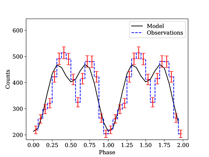
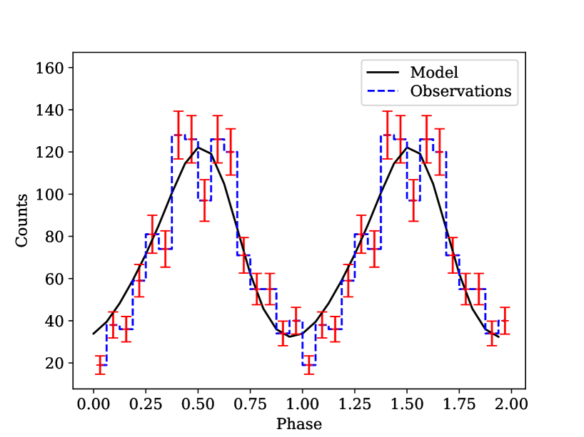
Fig. 3: Folded soft X-ray light-curve (300-2000 eV) for magnetars. Left panel: SGR0501, right panel 3XMM J185246.6+003317. Dashed blue lines show observations, and the theoretical light-curve for the most favourable orientation is shown with black solid lines. Red error bars are $1\sigma$ confidence intervals.

Data Availability Statement

The data that support the plots within the paper and other findings are available from the corresponding authors upon reasonable request.

Code Availability Statement

The codes that were used to prepare our models within the paper are available from the corresponding authors upon reasonable request.

Correspondence

Correspondence should be addressed to Andrei Igoshev and Rainer Hollerbach.

Acknowledgements

This work was supported by STFC grant No. ST/S000275/1. The numerical simulations were carried out on the STFC-funded DiRAC I UKMHD Science Consortia machine, hosted as part of and enabled through the ARC3 HPC resources and support team at the University of Leeds.

Contributions

All authors contributed to the simulation design, interpretation and writing the manuscript. A.P.I. carried out the X-ray data reduction, the MHD simulations and the model fitting. T.S.W. adapted the PARODY code to solve magneto-thermal equations.

Competing financial interests

The authors declare no competing financial interests.

References

- 1 Victoria M. Kaspi and Andrei M. Beloborodov. Magnetars. Ann. Rev. Astron. Astroph. , 55(1):261–301, Aug 2017.
- 2 Christopher Thompson and Robert C. Duncan. The Soft Gamma Repeaters as Very Strongly Magnetized Neutron Stars. II. Quiescent Neutrino, X-Ray, and Alfven Wave Emission. Astrophys. J., 473:322, Dec 1996.
- 3 José A. Pons and Daniele Viganò. Magnetic, thermal and rotational evolution of isolated neutron stars. Living Reviews in Computational Astrophysics, 5(1):3, December 2019.
- 4 Lilia Ferrario, Andrew Melatos, and Jonathan Zrake. Magnetic Field Generation in Stars. SSRv, 191(1-4):77–109, October 2015.
- 5 Jonathan Braithwaite and Hendrik C. Spruit. A fossil origin for the magnetic field in A stars and white dwarfs. Nature, 431(7010):819–821, October 2004.
- 6 J. Braithwaite and Å. Nordlund. Stable magnetic fields in stellar interiors. Astron. Astrophys. , 450(3):1077–1095, May 2006.
- 7 James E. Gunn and Jeremiah P. Ostriker. Magnetic Dipole Radiation from Pulsars. Nature, 221(5179):454–456, February 1969.
- 8 C. Thompson, M. Lyutikov, and S. R. Kulkarni. Electrodynamics of Magnetars: Implications for the Persistent X-Ray Emission and Spin-down of the Soft Gamma Repeaters and Anomalous X-Ray Pulsars. Astrophys. J., 574(1):332–355, July 2002.
- 9 Maxim Lyutikov and Fotis P. Gavriil. Resonant cyclotron scattering and Comptonization in neutron star magnetospheres. Mon. Not. Roy. Astron. Soc. , 368(2):690–706, May 2006.
- 10 N. Rea, S. Zane, R. Turolla, M. Lyutikov, and D. Götz. Resonant Cyclotron Scattering in Magnetars’ Emission. Astrophys. J., 686(2):1245–1260, October 2008.
- 11 Chin-Ping Hu, C. Y. Ng, and Wynn C. G. Ho. A systematic study of soft X-ray pulse profiles of magnetars in quiescence. Mon. Not. Roy. Astron. Soc. , 485(3):4274–4286, May 2019.
- 12 D. Viganò, N. Rea, J. A. Pons, R. Perna, D. N. Aguilera, and J. A. Miralles. Unifying the observational diversity of isolated neutron stars via magneto-thermal evolution models. Mon. Not. Roy. Astron. Soc. , 434(1):123–141, September 2013.
- 13 Feryal Özel, Dimitrios Psaltis, and Victoria M. Kaspi. Constraints on Thermal Emission Models of Anomalous X-Ray Pulsars. Astrophys. J., 563(1):255–266, December 2001.
- 14 T. S. Wood and R. Hollerbach. Three Dimensional Simulation of the Magnetic Stress in a Neutron Star Crust. Phys. Rev. Lett., 114(19):191101, May 2015.
- 15 Konstantinos N. Gourgouliatos and Rainer Hollerbach. Magnetic Axis Drift and Magnetic Spot Formation in Neutron Stars with Toroidal Fields. Astrophys. J., 852(1):21, January 2018.
- 16 K. N. Gourgouliatos and José A. Pons. Nonaxisymmetric Hall instability: A key to understanding magnetars. Physical Review Research, 1(3):032049, December 2019.
- 17 Konstantinos N. Gourgouliatos, Rainer Hollerbach, and Robert F. Archibald. Modelling neutron star magnetic fields. Astronomy and Geophysics, 59:5.37–42, 2018.
- 18 F. Camilo, J. Reynolds, S. Johnston, J. P. Halpern, and S. M. Ransom. The Magnetar 1E 1547.0-5408: Radio Spectrum, Polarimetry, and Timing. Astrophys. J., 679(1):681–686, May 2008.
- 19 Andrea Passamonti, Taner Akgün, José A. Pons, and Juan A. Miralles. On the magnetic field evolution time-scale in superconducting neutron star cores. Mon. Not. Roy. Astron. Soc. , 469(4):4979–4984, August 2017.
- 20 T. E. Riley, A. L. Watts, S. Bogdanov, P. S. Ray, R. M. Ludlam, S. Guillot, Z. Arzoumanian, C. L. Baker, A. V. Bilous, D. Chakrabarty, K. C. Gendreau, A. K. Harding, W. C. G. Ho, J. M. Lattimer, S. M. Morsink, and T. E. Strohmayer. A NICER View of PSR J0030+0451: Millisecond Pulsar Parameter Estimation. Astrophys. J. Lett., 887(1):L21, December 2019.
- 21 A. V. Bilous, A. L. Watts, A. K. Harding, T. E. Riley, Z. Arzoumanian, S. Bogdanov, K. C. Gendreau, P. S. Ray, S. Guillot, W. C. G. Ho, and D. Chakrabarty. A NICER View of PSR J0030+0451: Evidence for a Global-scale Multipolar Magnetic Field. Astrophys. J. Lett., 887(1):L23, December 2019.
- 22 Konstantinos N. Gourgouliatos, Toby S. Wood, and Rainer Hollerbach. Magnetic field evolution in magnetar crusts through three-dimensional simulations. Proceedings of the National Academy of Science, 113(15):3944–3949, April 2016.
- 23 Emmanuel Dormy, Philippe Cardin, and Dominique Jault. MHD flow in a slightly differentially rotating spherical shell, with conducting inner core, in a dipolar magnetic field. Earth and Planetary Science Letters, 160(1-2):15–30, July 1998.
- 24 Julien Aubert, Jonathan Aurnou, and Johannes Wicht. The magnetic structure of convection-driven numerical dynamos. Geophysical Journal International, 172(3):945–956, March 2008.
- 25 E. H. Gudmundsson, C. J. Pethick, and R. I. Epstein. Structure of neutron star envelopes. Astrophys. J., 272:286–300, September 1983.
- 26 Andrei M. Beloborodov. Gravitational Bending of Light Near Compact Objects. Astrophys. J. Lett., 566(2):L85–L88, Feb 2002.
- 27 M. van Adelsberg and D. Lai. Atmosphere models of magnetized neutron stars: QED effects, radiation spectra and polarization signals. Mon. Not. Roy. Astron. Soc. , 373(4):1495–1522, Dec 2006.
- 28 S. A. Olausen and V. M. Kaspi. The McGill Magnetar Catalog. Astrophys. J. Supp. Ser. , 212(1):6, May 2014.
- 29 W. Cash. Parameter estimation in astronomy through application of the likelihood ratio. Astrophys. J., 228:939–947, Mar 1979.
- 30 J. A. Nelder and R. Mead. A Simplex Method for Function Minimization. The Computer Journal, 7(4):308–313, 01 1965.