A residual concept for Krylov subspace evaluation of the $\varphi$ matrix function

Abstract

An efficient Krylov subspace algorithm for computing actions of the $\varphi$ matrix function for large matrices is proposed. This matrix function is widely used in exponential time integration, Markov chains and network analysis and many other applications. Our algorithm is based on a reliable residual based stopping criterion and a new efficient restarting procedure. For matrices with numerical range in the stable complex half plane, we analyze residual convergence and prove that the restarted method is guaranteed to converge for any Krylov subspace dimension. Numerical tests demonstrate efficiency of our approach for solving large scale evolution problems resulting from discretized in space time-dependent PDEs, in particular, diffusion and convection–diffusion problems.

65F60; 65M20; 65L05

1 Introduction

Exponential time integration is an actively developing research field [41], with numerous successful applications in challenging large scale computations, such as elastic wave equations [43], wind farm simulations [30], power delivery network analysis [69], large circuit analysis [70] vector finite element discretizations of Maxwell’s equations [12] and photonic crystal modeling [9, 11].

In this paper we propose a Krylov subspace method for solving initial-value problem (IVP)

(1) $$y^{\prime}(t)=-Ay(t)+g,\quad y(0)=v,\quad t\geqslant 0,$$

where the matrix $A\in\mathbb{R}^{n\times n}$ and vectors $g,v\in\mathbb{R}^{n}$ ($g\neq 0$) are given and the problem size $n$ is supposed to be large, i.e., $n\gg 1$. Using the variation of constants formula (see, e.g., [45, Chapter 2.3])

$$y(t)=\exp(-tA)v+\left[\int_{0}^{t}\exp(-(t-s)A)\,ds\right]g,\quad t\geqslant 0,$$

we can write $y(t)$ in the form

(2) $$y(t)=v+t\varphi(-tA)(g-Av),\quad t\geqslant 0.$$

Here $\varphi(-tA)(g-Av)$ is a matrix-vector product with the matrix function $\varphi(-tA)$ and $\varphi$ is defined as

(3) $$\varphi(z)\equiv\frac{e^{z}-1}{z},\quad z\in\mathbb{C},$$

where we set $\varphi(0)=1$ so that $\varphi$ is an entire function. Thus, the matrix function $\varphi$ provides the exact solution (2) to system (1). In other words, solving IVP (1) is equivalent to evaluating the matrix function $\varphi$ times a vector in (2). The method for solving (1) we propose in this paper is based on an efficient Krylov subspace evaluation of the matrix function $\varphi(-tA)$ in (2).

For homogeneous ODEs (ordinary differential equations), i.e., for $g=0$, the exact solution of (1) takes the well-known form $y(t)=\exp(-tA)v$. Therefore, computing matrix-vector products with the matrix function $\varphi$ and the matrix exponential is an important task in exponential time integration [41], occurring independently as well as within higher-order ODE Krylov subspace methods [42, 32] or splitting schemes [36, 8]. For large problems a direct evaluation of the matrix function based on dense linear algebra techniques [50, 37] is out of question. Therefore, the matrix-vector products with the matrix function are approximately computed, rather than the matrix function itself. Krylov subspace methods have been a successful tool for doing this since the end of the eighties; we list chronologically [54, 65, 23, 46, 57, 24, 39]. This progress in numerical linear algebra has triggered advances in numerical time integration methods (see, e.g., [31, 40, 18]) and a revival of the exponential time integrators [41], which have been developed since the sixties [19, 49, 48].

In this work we are interested in solving large scale problems (1) which result, for instance, within a method of lines, when spatially discretized PDEs (partial differential equations) have to be efficiently solved in time. This means that $A$ does not have to be symmetric and is often far from a normal matrix. Furthermore, fine and nonuniform grids as well as realistic coefficient values in the PDE may lead to a stiffness in the problem, i.e., the eigenvalues of $A$ may significantly vary in magnitude [29]. Taking into account unavoidable space discretization errors, error produced by a time integrator does not have to be extremely small in these problems. Usually absolute time errors in the range $[10^{-7},10^{-3}]$ suffice and this is the range we aim here. As we see in numerical tests, delivering accuracies in this range can be a challenge for existing exponential solvers. The proposed method appears to carry out this task successfully.

Krylov subspace exponential integrators are good candidates for solving large scale problems with sparse nonnormal matrices $A$, such as space-discretized PDEs. Indeed, these solvers have sufficient stability properties and often lead to an efficient compromise between standard implicit time integrators (which may occur too expensive in large scale applications) and explicit stabilized solvers. Moreover, as Krylov subspace methods can significantly profit from eigenvalue clustering [67], their application for solving stiff problems can be successful [33, 20, 16, 15] because stiffness typically means a large discrepancy in eigenvalues. Other approaches, not employing Krylov subspaces, for evaluating matrix exponential and related matrix functions of large sparse matrices include the Chebyshev polynomials, scaling and squaring with Taylor or Padé approximations and contour integrals [64, 21, 59, 17, 4].

Our approach for computing $\varphi$ matrix-vector products is essentially based on two ingredients presented in this paper: (i) a residual notion for $\varphi$ matrix functions and (ii) a restarting, i.e., an algorithm aiming to preserve convergence while keeping the Krylov dimension $k$ bounded, $k\leqslant k_{\max}$ [25]. The residual notion leads to a reliable stopping criterion and facilitates the proposed restarting. Restarting is often indispensable for solving large scale problems because the size $n$ of the matrix $A$ tends to be extremely large in real life applications. Thus, storing $k_{\max}$ Krylov basis vectors of size $n$ can be prohibitively expensive for $n\gg 1$ even if $k_{\max}$ is moderately large. Therefore, in the tests we restrict $k_{\max}$ by $30$. Numerous restarting algorithms for Krylov subspace evaluations of the matrix exponential have been proposed, for instance [2, 18, 26, 52, 10]. Restarting for general matrix functions include [27, 35]. Two restarting techniques have been designed specifically for the $\varphi$ matrix functions, namely [60] and [53]. They both are based on error estimates and choose a time interval length $t$ such that solving (1) by $k_{\max}$ Krylov steps yields a sufficiently small error. In the numerical experiments presented below we show that our method performs favorably compared to the codes based on these techniques.

Furthermore, we provide convergence analysis of the method, obtaining upper bounds for the residual norm with no asymptotic estimates involved, and show that the restarted algorithm is guaranteed to converge for any restart length, i.e., for any Krylov dimension $k_{\max}$.

The structure of this paper is as follows. In Section 2 we describe details of the Krylov subspace approximation and introduce a residual concept for the $\varphi$ matrix function. In Section 3 some observations on the residual behavior are given and the restarting algorithm, based on the observed behavior, is formulated. Section 4 is devoted to residual convergence analysis for both symmetric and nonsymmetric matrices. Based on this analysis, in Section 5 we show convergence of the restarted algorithm. Section 6 presents numerical experiments. Finally, some conclusions are drawn in Section 7.

2 Krylov subspace evaluations of the $\varphi$ matrix function

2.1 Residual notion for the $\varphi$ matrix function

Throughout the paper we assume that

(4) $$\mathrm{Re}(z^{*}Az)\geqslant 0,\quad\forall z\in\mathbb{C}^{n},$$

where the function $\mathrm{Re}(\cdot)$ is the real part of its argument, and, unless reported otherwise, $\|\cdot\|$ denotes the vector or matrix 2-norm.

To keep our presentation simpler, we first assume that the initial value vector in (1) is zero: $v=0$. In this case relation (2) takes a form

(2^′) $$y(t)=t\varphi(-tA)g,\quad t\geqslant 0,$$

and, thus, to solve (1) we have to evaluate the action of the matrix function $\varphi(-tA)$ on the vector $g$. Let upper Hessenberg matrix $\underline{H}_{k}\in\mathbb{R}^{(k+1)\times k}$ and matrix

$$V_{k+1}=\begin{bmatrix}v_{1}&v_{2}&\dots&v_{k}&v_{k+1}\end{bmatrix}\in\mathbb{R}^{n\times(k+1)},\qquad v_{1}=g/\|g\|,$$

with orthonormal columns $v_{j}$, be the matrices which result after carrying out $k$ steps of the Arnoldi process. These matrices satisfy the Arnoldi decomposition [34, 55, 67, 58]

(5) $$AV_{k}=V_{k+1}\underline{H}_{k}=V_{k}H_{k}+h_{k+1,k}v_{k+1}e_{k}^{T}.$$

Here $H_{k}=V_{k}^{T}AV_{k}\in\mathbb{R}^{k\times k}$ consists of the first $k$ rows of $\underline{H}_{k}$ and the columns $v_{1}$, …, $v_{k}$ span the Krylov subspace

$$\mathcal{K}_{k}(A,g)=\mathrm{span}(g,Ag,\dots,A^{k-1}g).$$

A standard way to compute a Krylov subspace approximation $y_{k}(t)$ to $y(t)$ in (2^′) is to set [67, Chapter 11]

(6) $$y_{k}(t):=V_{k}t\varphi(-tH_{k})(\beta e_{1}),$$

with $\beta=\|g\|$ and $e_{1}=[1,0,\dots,0]^{T}\in\mathbb{R}^{k}$. This expression for $y_{k}(t)$ can be derived by projecting the IVP (1) onto the Krylov subspace $\mathcal{K}_{k}(A,g)=\mathrm{colspan}(V_{k})$ in the Galerkin sense. Indeed, let us define a residual $r_{k}(t)$ of $y_{k}(t)$ with respect to (1), i.e., let

(7) $$r_{k}(t)\equiv-Ay_{k}(t)+g-y_{k}^{\prime}(t).$$

Now consider

$$y_{k}(t)\approx y(t),\qquad y_{k}(t)=V_{k}u(t)$$

such that its residual is kept orthogonal to the Krylov subspace: $V_{k}^{T}r_{k}(t)=0$. Since $g=\beta V_{k}e_{1}$, this orthogonality condition leads to a projected IVP in $u(t):\mathbb{R}\rightarrow\mathbb{R}^{k}$

(8) $$u^{\prime}(t)=-H_{k}u(t)+\beta e_{1},\qquad u(0)=0,$$

where $u(0)=0$ follows from the assumption $y(0)=0$. With $u(t)=t\varphi(-tH_{k})(\beta e_{1})$, we see that $V_{k}u(t)$ yields (6).

Now it is easy to observe that the residual (7) is readily computable in the course of the Arnoldi process:

(9) $$r_{k}(t) \stackrel{{\scriptstyle\eqref{yk}}}{{=}}-AV_{k}u(t)+g-V_{k}u^{\prime}(t)\stackrel{{\scriptstyle\eqref{ivp1}}}{{=}}-AV_{k}u(t)+g-V_{k}(-H_{k}y(t)+\beta e_{1})$$

$$=-AV_{k}u(t)+g+V_{k}H_{k}u(t)-g\stackrel{{\scriptstyle\eqref{Arn}}}{{=}}-h_{k+1,k}v_{k+1}e_{k}^{T}u(t),$$

where the bracketed numbers above the equality signs indicate the relations used in the derivation.

In case the initial value vector $v$ in (1) is not zero, we introduce a function $\tilde{y}(t)=y(t)-v$ which satisfies an IVP

$$\tilde{y}^{\prime}(t)=-A\tilde{y}(t)+\tilde{g},\quad\tilde{y}(0)=0,\quad t\geqslant 0,$$

with $\tilde{g}=g-Av$. Using (2) for this transformed problem we see that $\tilde{y}(t)=t\varphi(-tA)\tilde{g}$ and, thus, a Krylov subspace approximation $\tilde{y}_{k}(t)$ to $\tilde{y}(t)$, as well as its residual $\tilde{r}_{k}(t)$ (cf. (7)), can be computed as discussed above. Our Krylov subspace approximation to $y(t)$ is then $y_{k}(t)=\tilde{y}_{k}(t)+v$. For this approximation we introduce the residual $r_{k}(t)$ in the same way as for the case $v=0$: see (7). Then we have

$$r_{k}(t)=-Ay_{k}(t)+g-y_{k}^{\prime}(t)=-A\tilde{y}_{k}(t)-Av+g-y_{k}^{\prime}(t)=-A\tilde{y}_{k}(t)+\tilde{g}-\tilde{y}_{k}^{\prime}(t)=\tilde{r}_{k}(t),$$

i.e., the residual $r_{k}(t)$ coincides with the residual $\tilde{r}_{k}(t)$ for the transformed solution $\tilde{y}_{k}(t)$ and, hence, is also easily computable.

Note that the error $\epsilon_{k}(t)\equiv y(t)-y_{k}(t)$ of the Krylov approximation $y_{k}(t)$ satisfies an IVP

(10) $$\epsilon_{k}^{\prime}(t)=-A\epsilon_{k}(t)+r_{k}(t),\quad\epsilon_{k}(0)=0.$$

This shows that the introduced residual can be seen as the backward error for the approximate solution $y_{k}(t)$. This is similar to the well known property of the linear system residual: if $\tilde{x}$ approximates exact solution $x$ of a linear system $Ax=b$ then for its residual $\tilde{r}=b-A\tilde{x}$ we have $A(x-\tilde{x})=\tilde{r}$. Using (4),(10) we can bound the error norm as [10, Lemma 4.1]

(11) $$\|\epsilon_{k}(t)\|\leqslant t\varphi(-t\omega)\max_{s\in[0,t]}\|r_{k}(s)\|,$$

where $\omega\geqslant 0$ is a constant introduced below in (12). Hence, any residual estimates, including obtained below in Section 4 can be regarded as error estimates as well. This backward error property is also shared by the matrix exponential residual, see e.g. [10].

2.2 $\varphi$ via the matrix exponential, two approaches

If $A$ is nonsingular, a naive approach to compute $y:=\varphi(-A)g$ for a given $g$ would be to solve $v$ from $Av=-g$ and evaluate $y:=\exp(-A)v-v$. This means that we replace (1) by an equivalent IVP with the initial value $v$ and a zero source term. Comparing this approach with Krylov subspace evaluation of $y:=\varphi(-A)g$ shows that both Krylov subspace methods (for $y:=\exp(-A)v-v$ and for $y:=\varphi(-A)g$) require approximately the same number of Krylov steps. However, the additional computational costs for solving $Av=-g$ are not paid off. Hence, unless the systems with $A$ can be solved at a negligible cost, computing actions of $\varphi$ by the matrix exponential actions appears to be inefficient. Of course, this approach can not be used for a general $g$ in case $A$ is singular.

We remark that quite a different and successful approach to compute the $\varphi$ matrix function via a matrix exponential is presented in [57, Proposition 2.1] (see also [4]). For computing $\varphi(-tA)v$, $A\in\mathbb{R}^{n\times n}$, it amounts to evaluating the last column of $\exp(-t\widehat{A})$, where $\widehat{A}\in\mathbb{R}^{(n+1)\times(n+1)}$ is a matrix obtained by augmenting $A$ with $v$ as the last column and zeros as the last row. In the context of large scale problems and Krylov subspace methods this approach has a drawback that eventual (skew) symmetry of $A$ is lost in $\widehat{A}$. We use this approach for the evaluating $u(t)=t\varphi(-tH_{k})(\beta e_{1})$ to solve the small scale projected IVP (8), see Section 6.

3 A restarting procedure for $\varphi$ Krylov subspace evaluation

3.1 The residual norm as a function of time

For real matrices $A$ it is not difficult to see that property (4) is equivalent to

$$x^{T}Ax\geqslant 0,\quad\forall x\in\mathbb{R}^{n},$$

which means that the symmetric part $\frac{1}{2}(A+A^{T})$ of $A$ is nonnegative definite. Denote

(12) $$\omega\equiv\min_{0\neq x\in\mathbb{R}^{n}}\frac{x^{T}Ax}{x^{T}x}\geqslant 0.$$

Then it holds (see, e.g., [45, Section I.2.3])

(13) $$\|\exp(-tA)\|\leqslant e^{-t\omega},\qquad\forall t\geqslant 0.$$

A similar estimate holds for the matrix $H_{k}=V_{k}^{T}AV_{k}$ produced by the Arnoldi process (see (5)). Indeed, let

(14) $$\omega_{k}\equiv\min_{0\neq y\in\mathbb{R}^{k}}\frac{y^{T}H_{k}y}{y^{T}y}.$$

Then

$$\omega_{k}=\min_{0\neq y\in\mathbb{R}^{k}}\frac{(V_{k}y)^{T}A(V_{k}y)}{y^{T}y}\geqslant\omega\geqslant 0,$$

so that, similarly to (13),

(15) $$\|\exp(-tH_{k})\|\leqslant e^{-t\omega_{k}},\qquad\forall t\geqslant 0.$$

Exploiting the estimate [41, Proof of Lemma 2.4]

$$\|\varphi(-tA)\|\leqslant\int_{0}^{1}\|\exp(-t(1-\theta)A)\|\,d\theta,$$

bounding the norm under the integral by $e^{-t(1-\theta)\omega}$ and evaluating the integral, we obtain a useful inequality

(16) $$\|\varphi(-tA)\|\leqslant\varphi(-t\omega).$$

Then a similar relation holds also for $H_{k}$:

(17) $$\|\varphi(-tH_{k})\|\leqslant\varphi(-t\omega_{k}).$$

Proposition 3.1.

Let $t>0$, $g\in\mathbb{R}^{n}$ and let $A\in\mathbb{R}^{n\times n}$ be such that (4) holds. If $y_{k}(t)$ is the Krylov subspace approximation (6) to the vector $y(t)=t\varphi(-tA)g$ then for its residual $r_{k}(t)$, defined by (7), (9), holds

(18) $$\|r_{k}(t)\|\leqslant\beta th_{k+1,k}\varphi(-t\omega_{k})=\begin{cases}\dfrac{\beta}{\omega_{k}}h_{k+1,k}(1-e^{-t\omega_{k}}),\quad&\text{for }\omega_{k}>0,\\ \beta th_{k+1,k},\quad&\text{for }\omega_{k}=0,\end{cases}$$

where $\omega_{k}$ is defined by (14).

Proof 3.2.

From (8) we have $u(t)=t\varphi(-tH_{k})(\beta e_{1})$, so that

$$\|u(t)\|\leqslant\beta t\|\varphi(-tH_{k})\|\leqslant\beta t\varphi(-t\omega_{k})=\begin{cases}\dfrac{\beta}{\omega_{k}}(1-e^{-t\omega_{k}}),\quad&\text{for }\omega_{k}>0,\\ \beta t,\quad&\text{for }\omega_{k}=0,\end{cases}$$

where (17) is used. Relation (9) implies

$$\|r_{k}(t)\|=h_{k+1,k}\,|e_{k}^{T}u(t)|\leqslant h_{k+1,k}\|u(t)\|,$$

where $h_{k+1,k}\geqslant 0$ is guaranteed by the Arnoldi process. The last relation, together with the above estimate on $\|u(t)\|$, gives the required bound (18).

Note that (18) exhibits solely the time behavior of the residual $r_{k}(t)$ as a function of time for a fixed $k$. A more detailed analysis of the residual dependence on $k$ and on $t$ is given below in Section 4.

3.2 Residual-time (RT) restarting procedure

The method for evaluating the $\varphi$ matrix functions we propose in this paper adopts the so-called residual-time (RT) restarting strategy. It is proposed for the matrix exponential evaluations in our recent paper [13]. The RT strategy is essentially based on a notion of the matrix exponential residual defined, for an approximation $w_{k}(t)\approx w(t)=\exp(-tA)v$, as [18, 22, 10]

$$-Aw_{k}(t)-w_{k}^{\prime}(t).$$

The RT restarting is based on the observation that the residual is easily computable and the residual norm tends to be a monotonically increasing function of time, which explains the name “residual-time” restarting. The $\varphi$ residual (7) exhibits the same behavior (see relation (9) and Proposition 3.1 above). Therefore the RT restarting approach can be readily adopted for the $\varphi$ evaluations.

The RT restarting approach is quite simple. We solve (1) by performing $k=1,2,\dots,k_{\max}$ steps of the Arnoldi process (see Section 2.1). We stop as soon as the residual norm $\max_{s\in[0,t]}\|r_{k}(s)\|$ is small enough. If, after $k_{\max}$ carried out steps, this is not the case we find a time moment $\delta$ such that the residual norm $\|r_{k_{\max}}(s)\|$ is sufficiently small for $s\in[0,\delta]$. Then we set in (1) $v:=y_{k}(\delta)$, decrease the time interval $t:=t-\delta$ and start the Arnoldi process for this modified IVP again. This RT restarting for the $\varphi$ matrix function evaluations is outlined in Figure 1.

% Given: $A\in\mathbb{R}^{n\times n}$, $g\neq 0$, $v\in\mathbb{R}^{n}$, $t>0$, $k_{\max}$ and $\mathtt{tol}>0$

$\mathtt{convergence}:=\mathtt{false}$, $\mathtt{tol}:=\mathtt{tol}/t$

while not($\mathtt{convergence}$)

$\beta:=\|g-Av\|$, $v_{1}:=\frac{1}{\beta}(g-Av)$

for $k=1,\dots,k_{\max}$

carry out step $k$ of Arnoldi process:

compute $v_{k+1}$ and $h_{1,k}$, …, $h_{k+1,k}$

if $\max_{s\in[0,t]}\|r_{k}(s)\|\leqslant\mathtt{tol}$ then $(*)$

$\mathtt{convergence}:=\mathtt{true}$

break (leave the for loop)

elseif $k=k_{\max}$

% -------- restart after $k_{\max}$ steps

find largest $\delta$ such that $\max_{s\in[0,\delta]}\|r_{k}(s)\|\leqslant\mathtt{tol}$ $(\circ)$

$u:=\delta\varphi(-\delta H_{k})e_{1}$

$v:=v+V_{k}(\beta u)$

$t:=t-\delta$

break (leave the for loop)

end if

end for

end while

$u:=t\varphi(-tH_{k})e_{1}$, $y_{k}:=v+V_{k}(\beta u)$

Figure 1: Description of the RT (residual–time) restarting algorithm for the $\varphi$ matrix function evaluations. The algorithm computes Krylov subspace approximation $y_{k}(t)\approx v+\varphi(-tA)(g-Av)$ such that for its residual $r_{k}(t)$ holds $\max_{s\in[0,t]}\|r_{k}(s)\|\leqslant\mathtt{tol}$.

To monitor the values of the residual norm in the algorithm (see the algorithm lines marked with $(*)$, $(\circ)$), we compute the exact solution $u(s)$ of the projected IVP (8) at time moments $s=\Delta t$, $2\Delta t$, $3\Delta t$, …. This is done by recursion

(19) $$u(s+\Delta t) =E_{k}u(s)+\Delta td_{k},$$

$$E_{k}=\exp(-\Delta tH_{k}),\quad d_{k}=\beta\varphi(-\Delta tH_{k})e_{1},$$

where the matrix $E_{k}$ and vector $d_{k}$ are computed once. The value of $\Delta t$ is chosen in lines $(*)$ and $(\circ)$ differently:

(20) $$\Delta t:=\begin{cases}t/6,\quad&\text{to estimate }\displaystyle\max_{s\in[0,t]}\|r_{k}(s)\|,\text{ line }(*),\\ \dfrac{t}{2^{p}100},\quad&\text{with smallest }p=0,1,\dots\text{ such}\\ &\text{that }\|r_{k}(\Delta t)\|\leqslant\mathtt{tol},\text{ line }(\circ).\end{cases}$$

For estimating $\max_{s\in[0,t]}\|r_{k}(s)\|$ in line $(*)$ of the algorithm, $\Delta t$ does not have to be very small. This is because $\|r_{k}(s)\|$ usually achieves its maximum at the end point $s=t$ and the value $\|r_{k}(t)\|$ determines the quality of the approximation $y_{k}(t)\approx y(t)$. We emphasize that we compute the values of $u(s)$ exactly, and the computation accuracy does not depend on $\Delta t$ as is the case in a regular time integration scheme.

To determine the restart interval length $\delta$ (line $(\circ)$ in Figure 1), we proceed according to formula (20). More specifically, $\Delta t$ is initially set to $t/100$. If $\|r_{k}(\Delta t)\|\leqslant\mathtt{tol}$, we trace the values $\|r_{k}(\Delta t)\|$, $\|r_{k}(2\Delta t)\|$, …by recursion (19), until they exceed the tolerance value. Then we set $\delta$ to the largest $p\Delta t$ for which $\|r_{k}(p\Delta t)\|\leqslant\mathtt{tol}$. Otherwise, if $\|r_{k}(\Delta t)\|>\mathtt{tol}$ for $\Delta t=t/100$, we keep on halving $\Delta t$ until $\|r_{k}(\Delta t)\|\leqslant\mathtt{tol}$ and then set $\delta:=\Delta t$.

4 Estimates on the residual in terms of the Faber series

For simplification of formulae we assume in this section that $\beta=1$.

Faber series as a means to investigate convergence of Arnoldi’s method were introduced in [46]; see also [6].

4.1 A general estimate

Denote by $W(A)$ be the numerical range of matrix $A$ and let $\Phi_{j}$ be the Faber polynomials [63] for the compact $W(A)$. Since, for a fixed $t$, $\varphi(-tz)$ is an entire function of $z$, we can consider the Faber series decomposition

(21) $$f(z;t)\equiv t\varphi(-tz)=\frac{1-e^{-tz}}{z}=\sum_{j=0}^{+\infty}f_{j}(t)\Phi_{j}(z),\qquad z\in W(A),\quad t\geqslant 0,$$

where $t$ is considered as a parameter.

The following assertion is an analogue of [14, Proposition 1].

Proposition 4.1.

The residual (7) satisfies the inequality

(22) $$\|r_{k}(t)\|\leqslant 2h_{k+1,k}\sum_{j=k-1}^{+\infty}|f_{j}(t)|\leqslant 2\|A\|\sum_{j=k-1}^{+\infty}|f_{j}(t)|.$$

Proof 4.2.

The superexponential convergence in $j$ and the smoothness of $f_{j}(t)$ in $t$ enable one to differentiate series (21) in $t$. Decomposition (21) implies that the approximant (6) can be represented as

(23) $$y_{k}(t)=V_{k}f(H_{k};t)e_{1}=V_{k}\sum_{j=0}^{+\infty}f_{j}(t)\Phi_{j}(H_{k})e_{1}.$$

From (21) we see that

(24) $$e^{-tz}=1-zf(z;t)=1-\sum_{j=0}^{+\infty}f_{j}(t)z\Phi_{j}(z).$$

Therefore, since $\frac{\partial e^{-tz}}{\partial t}=-ze^{-tz}$, we obtain, differentiating (24),

$$-ze^{-tz}=\frac{\partial}{\partial t}\left[1-\sum_{j=0}^{+\infty}f_{j}(t)z\Phi_{j}(z)\right],$$

$$-z\left[1-\sum_{j=0}^{+\infty}f_{j}(t)z\Phi_{j}(z)\right]=-\sum_{j=0}^{+\infty}f_{j}^{\prime}(t)z\Phi_{j}(z),$$

$$1-\sum_{j=0}^{+\infty}f_{j}(t)z\Phi_{j}(z)=\sum_{j=0}^{+\infty}f_{j}^{\prime}(t)\Phi_{j}(z),$$

(25) $$-1+\sum_{j=0}^{+\infty}\left[f_{j}^{\prime}(t)+zf_{j}(t)\right]\Phi_{j}(z)=0.$$

Exploiting equality $\deg\Phi_{j}=j$ and relation (7), (23), (5), (4.2) with $H_{k}$ substituted for $z$, we get

$$r_{k}(t)=-\left(V_{k}H_{k}+h_{k+1,k}v_{k+1}e_{k}^{\mbox{\it\tiny T}}\right)\sum_{j=0}^{+\infty}f_{j}(t)\Phi_{j}(H_{k})e_{1}+g-V_{k}\sum_{j=0}^{+\infty}f_{j}^{\prime}(t)\Phi_{j}(H_{k})e_{1}$$

$$=-V_{k}\sum_{j=0}^{+\infty}\left[f_{j}^{\prime}(t)\mathcal{I}_{k}+H_{k}f_{j}(t)\right]\Phi_{j}(H_{k})e_{1}+V_{k}e_{1}-h_{k+1,k}v_{k+1}e_{k}^{\mbox{\it\tiny T}}\sum_{j=0}^{+\infty}f_{j}(t)\Phi_{j}(H_{k})e_{1}$$

$$=-h_{k+1,k}v_{k+1}e_{k}^{\mbox{\it\tiny T}}\sum_{j=k-1}^{+\infty}f_{j}(t)\Phi_{j}(H_{k})e_{1},$$

where $\mathcal{I}_{k}$ denotes the $k\times k$ identity matrix. The bound $\|\Phi_{j}(H_{k})\|\leqslant 2$ (see [5, Theorem 1]) now implies (22).

Remark 4.3.

Comparing estimate (22) and the estimate on the error

$$\|y(t)-y_{k}(t)\|\leqslant 4\sum_{j=k}^{+\infty}|f_{j}(t)|$$

(see [6, Theorem 3.2]) shows that the two upper bounds mainly differ in coefficients. Thus, we can conjecture that the error and the residual behave similarly to each other.

4.2 The symmetric case

We assume here that $A^{T}=A$ and the spectral interval of $A$ is contained in the segment $[0,2c]$, $c>0$. The change of variable $x=(z-c)/c$ translates $f(z;t)$ into the function

$$g(x;t)\equiv\frac{1-e^{-ct}e^{-ctx}}{c(x+1)},$$

and we wish to estimate its Chebyshev coefficients in $x$, because in this case the Faber series essentially reduces to the Chebyshev series up to a linear variable scaling. Following [56], we denote by $a_{m}[h]$ the $m$th Chebyshev coefficient of a function $h$ defined for $x\in[-1,1]$ as

$$h(x)=\sum_{m=0}^{+\infty}{\!}^{\prime}a_{m}[h]T_{m}(x),$$

where $T_{m}$ is the $m$th first kind Chebyshev polynomial and the prime ${}\prime$ means that the term at $m=0$ is divided by two.

Lemma 4.4.

For $k\geqslant 2$ the inequality

(26) $$\sum_{m=k-1}^{+\infty}\left|a_{m}\left[\frac{1-e^{-ct}e^{-ctx}}{c(x+1)}\right]\right|\leqslant\frac{2e^{-ct}}{c}\sum_{\nu=k}^{+\infty}(\nu-k+2)(\nu-k+1)I_{\nu}(ct).$$

holds with Bessel functions $I_{\nu}$.

Proof 4.5.

With formulae [56, Ch. II, § 11, (10), (54)], we have

$$e^{-ctx}=2\sum_{j=0}^{+\infty}{\!}^{\prime}I_{j}(-ct)T_{j}(x)=2\sum_{j=0}^{+\infty}{\!}^{\prime}(-1)^{j}I_{j}(ct)T_{j}(x).$$

Then, with $\delta_{i,j}$ denoting the Kronecker delta, we obtain

$$a_{m}\left[\frac{1-e^{-ct}e^{-ctx}}{c}\right]=\frac{2\delta_{m,0}-e^{-ct}a_{m}[e^{-ctx}]}{c}=\frac{2\delta_{m,0}-2(-1)^{m}e^{-ct}I_{m}(ct)}{c},$$

which in view of [56, Ch. II, § 9, Theorem 9.4, (42)] gives

$$a_{m}\left[\frac{1-e^{-ct}e^{-ctx}}{c(x+1)}\right]=2\sum_{l=0}^{+\infty}(-1)^{l}{l+1\choose 1}a_{m+l+1}\left[\frac{1-e^{-ct}e^{-ctx}}{c}\right]$$

$$=\frac{4}{c}\sum_{l=0}^{+\infty}(-1)^{l}(l+1)[\delta_{m+l+1,0}-e^{-ct}(-1)^{m+l+1}I_{m+l+1}(ct)]$$

$$=\frac{4}{c}(-1)^{m}\sum_{l=0}^{+\infty}(l+1)e^{-ct}I_{m+l+1}(ct),$$

whence

$$\sum_{m=k-1}^{+\infty}\left|a_{m}\left[\frac{1-e^{-ct}e^{-ctx}}{c(x+1)}\right]\right|\leqslant\frac{4e^{-ct}}{c}\sum_{m=k-1}^{+\infty}\sum_{l=0}^{+\infty}(l+1)I_{m+l+1}(ct)$$

$$=\frac{4e^{-ct}}{c}\sum_{\nu=k}^{+\infty}\left[\sum_{l=0}^{\nu-k}(l+1)\right]I_{\nu}(ct)=\frac{4e^{-ct}}{c}\sum_{\nu=k}^{+\infty}\frac{(\nu-k+2)(\nu-k+1)}{2}I_{\nu}(ct)$$

$$=\frac{2e^{-ct}}{c}\sum_{\nu=k}^{+\infty}(\nu-k+2)(\nu-k+1)I_{\nu}(ct).$$

Proposition 4.6 (A general error bound for the symmetric case).

For $k\geqslant 2$

(27) $$\|r_{k}(t)\|\leqslant 4e^{-ct}\sum_{\nu=k}^{+\infty}(\nu-k+2)(\nu-k+1)I_{\nu}(ct).$$

Proof 4.7.

Gathering (22), the definition of $c$, (26) and the fact that $\Phi_{[-1,1],\nu}=2T_{\nu}$, $\nu\geqslant 1$ (see [63, Ch. II, § 1, (21)]), derive

$$\|r_{k}(t)\|\leqslant 4c\sum_{j=k-1}^{+\infty}|f_{j}(t)|=2c\sum_{j=k-1}^{+\infty}\left|a_{j}\left[\frac{1-e^{-ct}e^{-ctx}}{c(x+1)}\right]\right|$$

$$\leqslant 4e^{-ct}\sum_{\nu=k}^{+\infty}(\nu-k+2)(\nu-k+1)I_{\nu}(ct).$$

A similar use of Bessel functions $I_{k}$ can be found in [23, § 4]. Here we have the term $(\nu-k+2)(\nu-k+1)$ as a complication. Note that the upper bound (27) can be easily computed with a high accuracy by truncating the infinite sum $\sum_{\nu=k}^{+\infty}$ to $\sum_{\nu=k}^{M}$ where $M$ can be estimated as discussed in [23, § 4]. Nevertheless, as Proposition 4.10 below shows, an explicit bound on the residual norm can be obtained from (27).

Lemma 4.8.

Let $\mu\in\mathbb{N}$ and $w\geqslant 0$. Then the Bessel function $I_{\mu}$ obeys the inequality

(28) $$e^{-w}I_{\mu}(w)\leqslant\frac{w^{\mu}}{(2\mu-1)!!}.$$

Proof 4.9.

Using formulae [1, 9.6.18, 6.1.8, 6.1.12], derive

$$e^{-w}I_{\mu}(w)\leqslant\frac{(w/2)^{\mu}}{\sqrt{\pi}\,\Gamma(\mu+1/2)}\left|\int\limits_{0}^{\pi}e^{w\cos\theta}\sin^{2\mu}\theta\,d\theta\right|\leqslant e^{-w}\frac{(w/2)^{\mu}}{\sqrt{\pi}\,\Gamma(\mu+1/2)}\,\pi e^{w}$$

$$=\frac{\sqrt{\pi}w^{\mu}}{2^{\mu}\cdot\frac{(2\mu-1)!!}{2^{\mu}}\cdot\sqrt{\pi}}=\frac{w^{\mu}}{(2\mu-1)!!}.$$

Proposition 4.10 (An error bound for $k$ of order at least $ct$ in the symmetric case).

If

(29) $$k\geqslant\max\{5ct,2\},$$

then

(30) $$\|r_{k}(t)\|\leqslant\frac{16(ct)^{k}}{(2k-1)!!}$$

Proof 4.11.

Exploiting assumption (29) and the inequality (see [51, Proposition 1])

$$I_{\nu+1}(w)<\frac{I_{\nu}(w)}{1+\frac{\nu}{w}},\qquad w>0,\qquad\nu\geqslant-1,$$

obtain for $\nu\geqslant k$

$$\frac{(\nu-k+3)(\nu-k+2)I_{\nu+1}(ct)}{(\nu-k+2)(\nu-k+1)I_{\nu}(ct)}=\left(1+\frac{2}{\nu-k+1}\right)\cdot\frac{I_{\nu+1}(ct)}{I_{\nu}(ct)}$$

$$<\frac{3}{1+\frac{\nu}{ct}}\leqslant\frac{3}{1+\frac{5ct}{ct}}\leqslant\frac{1}{2},$$

so that, in view of (28),

$$e^{-ct}\sum_{\nu=k}^{+\infty}(\nu-k+2)(\nu-k+1)I_{\nu}(ct)\leqslant e^{-ct}\cdot 4I_{k}(ct)\leqslant\frac{4(ct)^{k}}{(2k-1)!!}.$$

It remains to substitute the above bound into (27).

Proposition 4.10 is an analogue of [23, Theorem 5]. Bound (30) would be exponentially worse, if we used the Taylor series instead of the Chebyshev one; this clarifies the role of Faber series.

In Figure 2 we plot the graph of the right-hand side of (27) for the values $c$ and $t$ as occur in the numerical test presented in Section 6.1. Since $\|A\|_{2}^{2}\leqslant\|A\|_{1}\|A\|_{\infty}$ (see, e.g., [44, Chapter 5.6]) and $\|A\|_{1}=\|A\|_{\infty}$ for $A=A^{T}$, we can estimate $c$ by $\|A\|_{1}/2$. This leads to the $c$ values reported in caption of Figure 2. The $t$ values used in the plots (and reported in the caption) are taken to be approximately the average time interval length $\bar{\delta}$ per restart, i.e., $t:=\bar{\delta}$, obtained from data in Table 1 as the total time interval length divided by the number of restarts. In the figure we also plot the actual residual norm values computed with the regular Lanczos process.

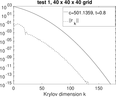
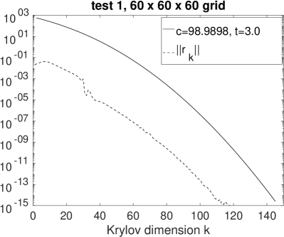
Figure 2: The solid lines are error upper bound (27) for $c=501.1359$, $t=\bar{\delta}=0.8$ (left plot) and $c=98.9898$, $t=\bar{\delta}=3.0$ (right plot). The values correspond to $A$ being discretized anisotropic elliptic operator described in Section 6.1, for $40\times 40\times 40$ (left plot) and $60\times 60\times 60$ (right plot) finite volume grids, respectively. The dashed lines are the actual scaled residual norm values $\|r_{k}\|/\beta$.

From Figure 2 we see that the obtained upper bound is far from being sharp. This is certainly expected. Although (27) is a true upper bound and contains no asymptotic estimates, it does not reflect the sensibility of the Krylov subspace methods with respect to the discrete structure of the spectrum. To confirm this and to show that the upper bound in (27) can be sharp, in Figure 3 we plot the upper bound along with the actual residual norm values for the following tridiagonal $A\in\mathbb{R}^{n\times n}$ and $g\in\mathbb{R}^{n}$:

(31) $$A=\begin{bmatrix}1&1/\sqrt{2}&0&\dots&0\\ 1/\sqrt{2}&1&1/2&\ddots&\vdots\\ 0&1/2&\ddots&\ddots&\\ \vdots&\ddots&\ddots&\ddots&\end{bmatrix},\quad g=\begin{bmatrix}1\\ 0\\ \vdots\\ 0\end{bmatrix}.$$

It can be shown that $\|A\|\approx 2$ for large $n$, hence, we take $n=1000$ and $c=1$. The residual values are computed with the regular Lanczos process. As we see from the plots, the upper bound (27) is sharp.

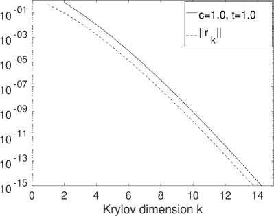
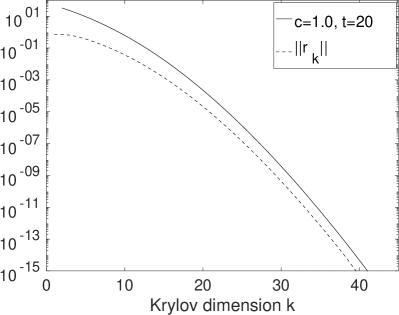
Figure 3: The solid lines are error upper bound (27) for $c=1$, $t=1$ (left plot) and $c=1$, $t=20$ (right plot). The values correspond to $A$ defined in (31). The dashed lines are the actual scaled residual norm values $\|r_{k}\|/\beta$ obtained for $g$ defined in (31).

4.3 A weakly non-symmetric case

Proposition 4.12 (An error bound for an “elliptic” numerical range).

Let the numerical range $W(A)$ be enlcosed by an ellipse $E_{c,\rho}$ with foci $0$ and $2c$ with the sum of semiaxes $\rho c$, $c>0$, $\rho>1$. Then for $k\geqslant 2$

(32) $$\|r_{k}(t)\|\leqslant 4e^{-ct}\sum_{\nu=k}^{+\infty}(\nu-k+2)(\nu-k+1)\rho^{\nu}I_{\nu}(ct).$$

Proof 4.13.

The proof is a slight generalization of that of proposition 4.6; the latter corresponds to the limit case $\rho=1$. One should exploit the relation (see [63, Ch. II, § 1, (25)]) between the Faber polynomials for $E_{c,\rho}$ and the Faber polynomials for the focal segment $[0,2c]$ (actually, the shifted Chebyshev polynomials).

Similarly to (27), upper bound (32) is easily computable by truncating the infinite series in (32).

In Figure 4 we plot the right-hand side of (32) for the matrices of the second and third test problems, see Sections 6.2 and 6.3. In each of these two test problems several grids and corresponding parameter settings are used, and the two matrices for the plots in Figure 4 are built for the grids $202\times 202$ (the second test) and $512\times 512$ (the third test), respectively. The $t$ values are approximate average time interval length $\bar{\delta}$ per restart, computed as the total time interval length divided by the number of restarts. To obtain the ellipse parameters appearing in the bound, we approximate the numerical ranges of the matrices $A$ by the numerical ranges of their Krylov projections $H_{k}=V_{k}^{T}AV_{k}$, see (5). This is done for a sufficiently large $k$ such that the exterior eigenvalues of $A$ are well approximated by the eigenvalues of $H_{k}$. Thus, the plots in Figure 4 are produced for approximate spectral data but do suffice for illustrative purposes. In the figure the actual residual norm is also plotted.

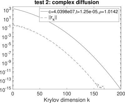
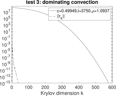
Figure 4: The solid lines are error upper bound (32) for $c={\tt 4.0398e07}$, $t=\bar{\delta}=\texttt{1.25e-05}$, $\rho=1.0142$ (left plot) and $c=0.49949$, $t=\bar{\delta}=3750$, $\rho=1.0937$ (right plot). The values correspond to the matrices $A$ of the second test problem (see Section 6.2, grid $202\times 202$) and the third test problem (see Section 6.3, grid $512\times 512$), respectively. The dashed lines are the actual scaled residual norm values $\|r_{k}\|/\beta$.

5 Convergence of the restarted method

Proposition 5.1.

Let the RT restarted Krylov subspace method be used to compute an approximation to the solution $y(t)$, $t<\infty$, of IVP (1) and let $\mathtt{tol}$ be the residual tolerance used at each restart. Then for any restart length $k_{\max}$ the RT restarted Krylov subspace method stops after a finite number $J$ of restarts and the error of its approximate solution $y_{k}(t)$ is bounded by $t\cdot\mathtt{tol}$,

$$\|y(t)-y_{k}(t)\|\leqslant t\cdot\mathtt{tol},$$

with $t$ being the length of the time interval on which problem (1) is solved.

Proof 5.2.

Based on Propositions 3.1, 4.6, 4.12, we know that at each restart $j$ a $\delta_{j}>0$ can be found such that the residual norm does not exceed any tolerance $\mathtt{tol}$ on the time interval of length $\delta_{j}$. Hence, since the time interval length $t$ is finite and is reduced at each restart by $\delta_{j}$, a finite number $J$ of restarts will suffice. The time interval after $j$ restarts is reduced from $[0,t]$ to $[0,t-(\delta_{1}+\dots+\delta_{j})]$ and $\sum_{j=1}^{J}\delta_{j}=t$.

To simplify the notation in the proof, by $y_{j}(s)$, $s\in[0,\delta_{j}]$ we denote the Krylov subspace solution which is obtained, with $k\leqslant k_{\max}$ steps of the Arnoldi process, at restart $j$ ($k<k_{\max}$ is possible only for $j=J$). We also denote the residual of $y_{j}(s)$ by $r_{j}(s)$. With this notation, $y_{j}(s)$ approximates the exact solution $y(\sum_{i=1}^{j-1}\delta_{i}+s)$ for $s\in[0,\delta_{j}]$ with residual $r_{j}(s)$ such that

$$\max_{s\in[0,\delta_{j}]}\|r_{j}(s)\|\leqslant\mathtt{tol}.$$

Then the approximate solution at the first restart is

$$y_{1}(\delta_{1})=v+\delta_{1}\varphi(-\delta_{1}A)(g-Av)+\epsilon_{1}(\delta_{1}),$$

where $\epsilon_{1}(s)$ is the error of the approximation $y_{1}(s)\approx y(s)$. Using (11) we can bound $\|\epsilon_{1}\|$ as

$$\|\epsilon_{1}(\delta_{1})\|\leqslant\delta_{1}\varphi(-\delta_{1}\omega)\max_{s\in[0,\delta_{1}]}\|r_{1}(s)\|\leqslant\delta_{1}\varphi(-\delta_{1}\omega)\cdot\mathtt{tol}\leqslant\delta_{1}\cdot\mathtt{tol},$$

where $\omega\geqslant 0$ is the constant from (12). To further simplify the notation, let us denote $\epsilon_{j}=\epsilon_{j}(\delta_{j})$ and $y_{j}=y_{j}(\delta_{j})$. Then at restart 2 we have

$$y_{2} =y_{1}+\epsilon_{1}+\delta_{2}\varphi(-\delta_{2}A)(g-A(y_{1}+\epsilon_{1}))+\epsilon_{2}$$

$$=\underbrace{y_{1}+\delta_{2}\varphi(-\delta_{2}A)(g-Ay_{1})}_{\text{exact solution}}+\,\underbrace{\delta_{2}\varphi(-\delta_{2}A)(-A\epsilon_{1})+\epsilon_{1}+\epsilon_{2}}_{\varepsilon_{2}},$$

where we denote all the error terms by $\varepsilon_{2}$. Now note that

$$\delta_{2}\varphi(-\delta_{2}A)(-A\epsilon_{1})+\epsilon_{1}=\exp(-\delta_{2}A)\epsilon_{1},$$

and, hence,

$$\varepsilon_{2}=\exp(-\delta_{2}A)\epsilon_{1}+\epsilon_{2},\quad\|\varepsilon_{2}\|\leqslant\|\epsilon_{1}+\epsilon_{2}\|\leqslant(\delta_{1}+\delta_{2})\cdot\mathtt{tol}.$$

Here we bound $\epsilon_{2}$ in the same way as $\epsilon_{1}$ and use estimate (13). Continuing in the same way, we obtain at the last restart $J$

$$\varepsilon_{J} =\exp(-(t-\delta_{1})A)\epsilon_{1}+\exp(-(t-\delta_{1}-\delta_{2})A)\epsilon_{2}+\dots$$

$$\phantom{=}+\exp\left(-(t-\sum_{j=1}^{J-1}\delta_{j})A\right)\epsilon_{J-1}+\epsilon_{J},$$

$$\|\varepsilon_{J}\| \leqslant\|\epsilon_{1}\|+\dots+\|\epsilon_{J}\|\leqslant(\delta_{1}+\dots+\delta_{J})\cdot\mathtt{tol}=t\cdot\mathtt{tol}.$$

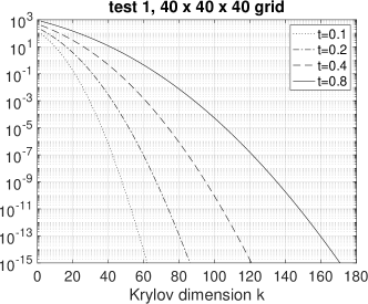
Figure 5: Residual upper bound (27) for $c=501.1359$ (the first test problem, $40\times 40\times 40$ grid) and different time interval lengths $t$.

The number of restarts $J$ appearing in Proposition 5, can be estimated from the residual upper bounds (27),(30),(32). This can be done, for example, using plots as shown in Figure 5. There, for the test problem described in Section 6.1, we plot the bound (27) for different time interval lengths $t$. For instance, if $k_{\max}\approx 30$ and the requested tolerance is in the range $[10^{-5},10^{-3}]$, then the restart interval length $\delta$ should be approximately $0.2$ (see the dotted curve in Figure 5). Hence, for the time interval length $t=1000$ used in the test, $J\approx 1000/0.2=5000$ restarts are expected. Since the bound (27) is not sharp, this should be seen as a safe, pessimistic estimate on $J$. Indeed, as we see from Table 1, the actual number of restarts is roughly four times smaller.

6 Numerical experiments

In the experiments presented here we test our method to compute actions of $\varphi(-tA)$ implemented with the proposed RT restarting. We compare our code phiRT with two other well known Krylov subspace codes for evaluating $\varphi(-tA)$, namely the phiv function of the EXPOKIT package [60] and the phip function presented in [53] and publicly available online. We do not include the recently proposed code phipm [53] in the comparisons because this code uses a variable Krylov dimension up to $100$. Using such a high Krylov dimension in the large scale problems is not always feasible, and in the tests we restrict the Krylov dimension for all the three solvers by $30$.

All the tests are carried out on a Linux laptop with four AMD Ryzen 3 3200U CPUs (clock rate 2.6 GHz) and 8 Gb memory, in Octave (version 4.2.2) with no parallelization. Our implementation of the Arnoldi and Lanczos processes does not include Krylov basis vector reorthogonalization and no serious orthogonality loss has been observed. In the numerical tests the Krylov subspace matrices are computed by the Lanczos process as soon as $A=A^{T}$, otherwise the Arnoldi process is employed.

To calculate matrix-vector products $\varphi(-tH_{k})x$ for the small projected Krylov subspace matrix $H_{k}$ in our algorithm (cf. (19)), we employ relation [57, Proposition 2.1]

$$\exp(\begin{bmatrix}-tH_{k}&x\\ 0&0\end{bmatrix})=\begin{bmatrix}\exp(-tH_{k})&\varphi(-tH_{k})x\\ 0&1\end{bmatrix},$$

computing the matrix exponential at the left hand side and, thus, reducing computations with $\varphi$ to computations with the matrix exponential (see also [4]). To compute the matrix exponentials $\exp(-tH_{k})$ here and in (19) the standard built-in function expm of Octave is used. It is based on Ward’s scaling and squaring method combined with diagonal Padé approximation and is certainly not the best method available, see [50, 38]. For the moderate tolerance range $[10^{-7},10^{-3}]$ we aim in the tests, we have observed no accuracy problems with this Octave implementation. We have chosen to stick to the built-in function expm to have our Octave code fully Matlab portable. Note that Matlab’s implementation of expm [3] is seen as more reliable but is not publicly available. For higher accuracy requirements we could switch, for instance, to the phipade function of the EXPINT package [7].

In all the tests the reported achieved error is measured for each of the three Krylov subspace solvers as

$$\frac{\|y_{k}(t)-y_{\mathrm{ref}}(t)\|}{\|y_{\mathrm{ref}}(t)\|},$$

where $y_{k}(t)$ is the solution of the Krylov subspace solver at final time $t$ and $y_{\mathrm{ref}}(t)$ is a reference solution computed with a high tolerance (reported for each test below) by the phiv function. Since the reference solution $y_{\mathrm{ref}}(t)$ is affected by the same space discretization error as $y_{k}(t)$, $\|y_{k}(t)-y_{\mathrm{ref}}(t)\|$ is a good indicator of the time error.

6.1 High-order discretized anisotropic elliptic operator

In this test we solve IVP (1) with a symmetric matrix $A$. It is a 3D (three-dimensional) anisotropic elliptic operator $10^{4}\partial_{xx}+10^{2}\partial_{yy}+\partial_{zz}$ with periodic boundary conditions defined in the spatial domain $[0,1]\times[0,1]\times[0,1]$ and discretized by a fourth order accurate finite volume discretization described in [68]. The source vector $g$ contains the grid values of either of the functions

$$\sin(2\pi x)\sin(2\pi y)\sin(2\pi z)+x(1-x)y(1-y)z(1-z),$$

$$\mathrm{e}^{-500((x-0.5)^{2}+(y-0.5)^{2}+(z-0.5)^{2}))}+x(1-x)y(1-y)z(1-z).$$

We use two different source vectors $g$ to make sure that Krylov subspace methods do not profit from a particular choice of the source vector. In this test the initial value vector $v$ in (1) is set to zero.

In the test we use uniform $40\times 40\times 40$ and $60\times 60\times 60$ grids, for which the problem size is $n=64\,000$ and $n=216\,000$, respectively. For these grids the matrix $A$ has its norms $\|A\|_{1}=\|A\|_{\infty}$ approximately equal to $1002.27$ and $197.98$, respectively. These values give the estimations $\|A\|_{1}/2$ of $c$ used in Figure 2. The final time is $t=1000$ and the reference solution is computed by function phiv with tolerance $\mathtt{tol}=\texttt{1e-11}$.

The results for this test are presented in Table 1 and in Figure 6, where for each of the solvers the values of achieved accuracy, the number of matrix-vector multiplications (matvecs) and the CPU times are given. These values are reported for the same tolerance 1e-6. Exploring performance of the solvers for different tolerance values leads to plots in Figure 6. As can be seen in the plots, on the coarser grid function phiv fails to produce results with an accuracy less stringent than $\approx 10^{-7}$. Its least accurate result (corresponding to the upper left end of the dashed curve) is obtained for tolerance 5e-2. An attempt to run the code with a less stringent tolerance 1e-1 yields an error message. Furthermore, the phip solver does not produce the results within the required accuracy range $[10^{-7},10^{-3}]$ and appears to be more expensive for this test than our phiRT. For both spatial grids the phip solver exhibits an abrupt change in the delivered accuracy with gradually varying requested tolerance, indicated in the Figure by segments AB and CD. Thus, we see that both phiv and phip solvers have difficulties with delivering results within the desired accuracy range $[10^{-7},10^{-3}]$.

Table 1: Results for the fourth order finite-volume discretized anisotropic heat equation

method(Krylov dim.),	delivered	matvecs /
requested tolerance	error	CPU time, s
$40\times 40\times 40$ grid, sine $g$
phiv($10$), 1e-06	3.05e-12	185472 / 1380
phip($10$), 1e-06	7.75e-14	170420 / 1282
phiRT($10$), 1e-06	1.37e-09	101487 / 824
phiv($30$), 1e-06	6.07e-13	61632 / 482
phip($30$), 1e-06	6.89e-14	79710 / 545
phiRT($30$), 1e-06	7.78e-09	33837 / 238
$40\times 40\times 40$ grid, Gaussian $g$
phiv($30$), 1e-06	1.33e-10	63520 / 565
phip($30$), 1e-06	9.98e-14	80910 / 572
phiRT($30$), 1e-06	8.56e-09	36117 / 324
$60\times 60\times 60$ grid, sine $g$
phiv($30$), 1e-06	2.40e-11	16800 / 692
phip($30$), 1e-06	2.91e-13	17640 / 525
phiRT($30$), 1e-06	1.59e-08	10191 / 258

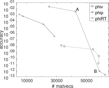
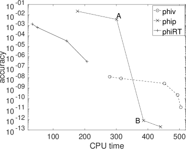
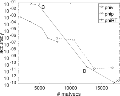
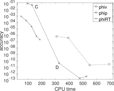
Figure 6: The fourth order finite-volume discretized anisotropic heat equation. Relative error versus number of the matrix-vector products (left) and versus the CPU time (right) for the phiv (dashed line), phip(dash-dotted line) and phiRT (solid line). The restart length is 30 for all the three solvers. The upper left end of the phiv curve at the top plots is obtained for tolerance 5e-02 and running phiv with tolerance 1e-01 fails with an error message. The points A, B, C, and D on the phip curve are obtained for the tolerances 5e-04, 1e-04, 3e-03, and 1e-03, respectively.

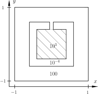
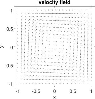
Figure 7: Diffusion coefficients $D_{1,2}(x,y)$ (left) and velocity field $[v_{1}(x,y),v_{2}(x,y)]$ (right). The region where $D_{1,2}=10^{3}$ occupies the square $[-0.4,0.4]\times[-0.4,0.4]$ and is surrounded by the wall where $D_{1,2}=10^{-4}$ which is $0.2$ wide and has a $0.1$ broad slit.

6.2 Convection–diffusion discretized by finite differences, complex diffusion

We now consider a nonsymmetric matrix $A$ resulting from a standard five point central-difference discretization of the following convection–diffusion operator:

$$L[u]=-(D_{1}u_{x})_{x}-(D_{2}u_{y})_{y}+\mathit{P\!e}{}\,\left(\frac{1}{2}(v_{1}u_{x}+v_{2}u_{y})+\frac{1}{2}((v_{1}u)_{x}+(v_{2}u)_{y})\right),$$

where $(x,y)\in[-1,1]\times[-1,1]$ and the homogeneous Dirichlet conditions are imposed on the boundary. Here the first derivatives representing the convective terms are written in a special way. If the velocity field is divergence-free, i.e., if $(v_{1})_{x}+(v_{2})_{y}=0$, then the central-difference discretization of the convective terms yields a skew-symmetric matrix [47]. This physically desirable property [68] guarantees that the first derivatives do not contribute to the symmetric part of the matrix which is the case for diffusive upwind discretizations.

The diffusion coefficients $D_{1,2}(x,y)$ are defined as shown at the left plot in Figure 7. This choice is inspired by [66, test 4]. The velocity field, taken as

$$v_{1}(x,y)=y(1-x^{2}),\qquad v_{2}(x,y)=x(y^{2}-1),$$

is the recirculating wind adopted from the IFISS package [62], see the right plot in Figure 7. The initial value vector $v$, cf. (1), has all its entries set to $0.01$. For $v=0$ the solution may become unstable due to appearance of small negative solution values (recall that central difference discretizations are used for both diffusion and convection terms). The components of the source vector $g$ are the values of function

$$1000\mathrm{e}^{-100(x^{2}+y^{2})}$$

on the finite difference grid. Uniform $202\times 202$, $402\times 402$ and $802\times 802$ grids are used in the experiments, so that the problem size is $n=40\,000$, $n=160\,000$ and $n=640\,000$, respectively. On the first two grids the Peclet number $\mathit{P\!e}$ is set to $10$, whereas $\mathit{P\!e}=20$ on the finest grid. For these Peclet values and all the three grids the ratio of the norms of the skew-symmetric and symmetric parts of the matrices, measured as the maximal row and column norms, is of order $10^{-5}$, i.e., the matrices are weakly nonsymmetric. Solution samples of this test problem can be seen in Figure 8. The reference solution is computed by the phiv function run with tolerance 1e-14.

The results of the comparison runs are presented in Table 2. To see clearly the dependence of the attained accuracy on the computational work and CPU time, we also present plots in Figure 9. We see that phiv tends to deliver a much more accurate solution than is requested by given tolerance. We also see that for the coarsest $202\times 202$ grid our solver is more efficient than phip in terms of matrix–vector multiplications but requires more CPU time. This effect disappears on the finer grids. There, for the moderate tolerance values we are interested in, phiRT clearly outperforms the other solvers in terms of CPU time and matrix–vector multiplications.

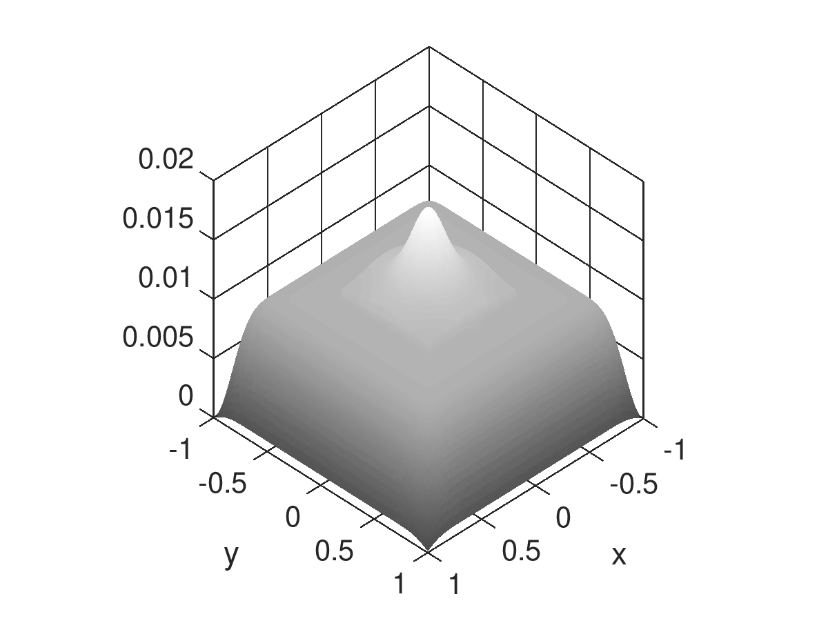
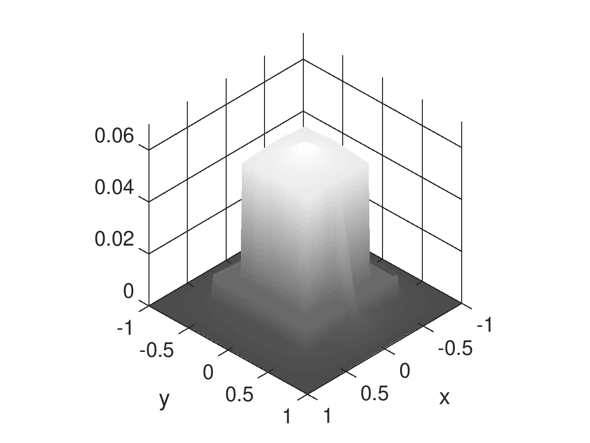
Figure 8: Solution of finite-difference discretized convection–diffusion problem at time $t=5\times 10^{-5}$ (left) and $t=10^{-3}$ (right), $202\times 202$ grid, $\mathit{P\!e}=10$. At the right plot a correspondence to the values of the diffusion coefficients $D_{1,2}$ is clearly visible, with a leakage through the slit, see Figure 7.

Table 2: Results for the finite-difference discretized convection–diffusion test problem.

method(Krylov dim.), delivered matvecs / requested tolerance error CPU time, s $202\times 202$ grid, $\mathit{P\!e}=10$, $t=10^{-3}$ phiv($30$), 5e-1 1.73e-08 6016 / 16.6 phiv($30$), 1e-1 1.66e-09 6528 / 18.2 phip($30$), 5e-1 1.67e-04 2700 / 8.1 phip($30$), 1e-1 8.16e-06 2850 / 8.6 phiRT($30$), 1e-2 1.36e-04 2368 / 9.2 phiRT($30$), 5e-3 3.80e-05 2399 / 9.6 $402\times 402$ grid, $\mathit{P\!e}=10$, $t=10^{-3}$ phiv($30$), 5e-1 8.80e-11 21856 / 328 phiv($30$), 1e-1 1.10e-11 23104 / 340 phip($30$), 5e-1 7.53e-07 9900 / 160 phip($30$), 1e-2 1.49e-06 13980 / 221 phiRT($30$), 1e-2 3.09e-04 6488 / 104 phiRT($30$), 1e-3 4.53e-06 10230 / 165 phiv($20$), 5e-1 1.53e-10 30756 / 342 phip($20$), 5e-1 8.21e-06 14520 / 177 phiRT($20$), 1e-2 4.50e-04 7433 / 95 phiRT($20$), 1e-3 9.78e-06 15012 / 183 $802\times 802$ grid, $\mathit{P\!e}=20$, $t=5\cdot 10^{-5}$ phiv($30$), 5e-1 3.22e-11 6304 / 463 phip($30$), 1e-1 5.03e-05 2310 / 186 phiRT($30$), 1e-2 3.51e-05 2100 / 167 phiv($20$), 1e-1 1.53e-11 8690 / 495 phip($20$), 1e-2 6.01e-06 4200 / 250 phiRT($20$), 1e-3 3.27e-06 3431 / 201

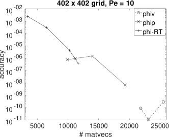
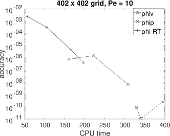
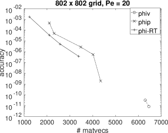
Figure 9: Finite-difference discretized convection–diffusion problem. Relative error versus number of the matrix-vector products (left) and versus the CPU time (right) for phiv (dashed line), phip (dash-dotted line) and phiRT (solid line). Top plots: $402\times 402$ grid, $\mathit{P\!e}=10$, $t=10^{-3}$, bottom plots: $802\times 802$ grid, $\mathit{P\!e}=20$, $t=5\cdot 10^{-5}$. The restart length is 30 for all the three solvers. The loosest tolerance value for phiv and phip solvers is 5e-01. Hence, it is problematic to obtain cheaper, less accurate results with these solvers.

6.3 Convection–diffusion discretized by finite elements, dominating convection

In this test IVP (1) is solved where $A$ and $g$ are produced by the IFISS software package [62, 61, 28]. More precisely, $A$ results from a finite-element discretization of the following two-dimensional convection–diffusion problem:

(33) $$-\nu\nabla^{2}u+\vec{w}\cdot\nabla u=0,\qquad u=u(x,y),\quad(x,y)\in[-1,1]\times[-1,1],$$

where $\nu$ is viscosity parameter and Dirichlet boundary conditions $u=0.5$ are imposed at all boundary points except for $y=1$, where

$$u(x,1)=\frac{1}{2}+\frac{1}{2}(1-x^{2}).$$

The initial value vector $v$ in (1) is set to zero in this test.

Discretization of (33) in IFISS by bilinear quadrilateral ($Q_{1}$) finite elements with the streamline upwind Petrov–Galerkin (SUPG) stabilization leads to a linear system $Au=g$, where $g$ enforces the Dirichlet boundary conditions. Thus, the IVP we solve is a nonstationary version of the stationary discretized convection–diffusion problem. We use uniform $512\times 512$ and $1024\times 1024$ grids with viscosity values $\nu=1/6400$ and $\nu=1/12800$, respectively. In both cases the maximum finite element grid Peclet number, estimated by IFISS as

$$\frac{1}{2\nu}\min\left\{\frac{h_{x}}{\cos\alpha},\frac{h_{y}}{\sin\alpha}\right\}\|\vec{w}\|_{2},\quad\alpha=\arctan\frac{w_{y}}{w_{x}},$$

is $\approx 25$, where $h_{x,y}$ and $w_{x,y}$ are respectively the element sizes and the components of the velocity $\vec{w}$.

For these viscosity values we have $\frac{1}{2}\|A+A^{T}\|_{1}=1$, $\frac{1}{2}\|A-A^{T}\|_{1}\approx 0.0078$ on the $512\times 512$ grid and $\frac{1}{2}\|A+A^{T}\|_{1}=1$, $\frac{1}{2}\|A-A^{T}\|_{1}\approx 0.0039$ on the $1024\times 1024$ grid. The length of the time interval is set to $t=2\cdot 10^{4}$. For this $t$ the solution $y(t)$ of IVP (1) still differs significantly from the stationary solution $A^{-1}g$ to which $y(t)$ converges for growing $t$, see Figure 10. The reference solution is computed by phiv with tolerance 1e-13.

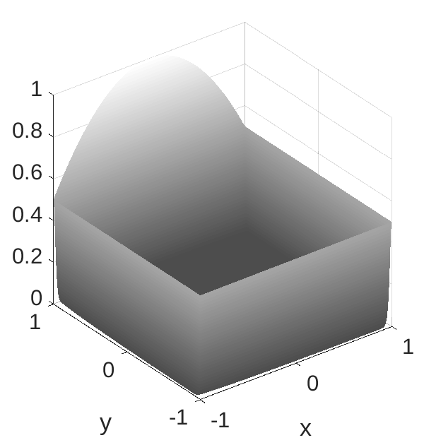
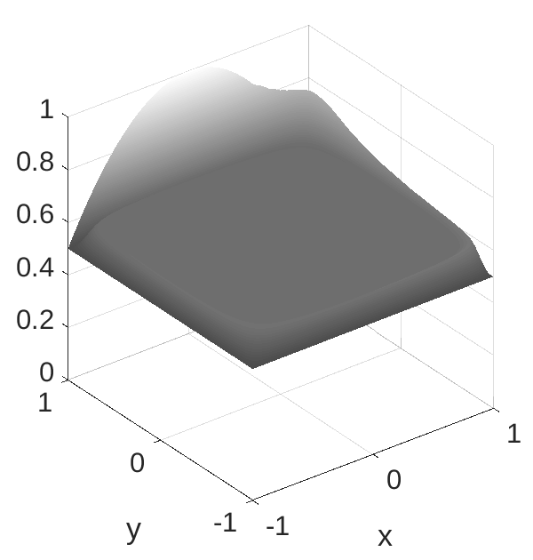
Figure 10: Solution of the IFISS convection-dominated problem $y(t)$ at $t=2\cdot 10^{4}$ (left) and the stationary solution $A^{-1}g$ (right) on the $512\times 512$ grid.

The results are presented in Tables 3 and 4 and in Figure 11. We see that phiRT appears to be more efficient for this test and that obtaining a time error within the desired tolerance range $[10^{-7},10^{-3}]$ can be problematic with phiv and phip. On both grids the phip solver demonstrates a remarkable “all-or-nothing” behavior: on the $1024\times 1024$ grid perturbing the requested tolerance from 7e-05 to 8e-05 yields a drop in the delivered accuracy from 8.15e-07 to 5.36e-01. This last accuracy value is not plotted in Figure 11 as it is too low for a satisfactory PDE solution.

Table 3: Results for the finite-element discretized convection-dominated convection–diffusion test problem, $\nu=1/6400$, $512\times 512$ grid

method(Krylov dim.), delivered matvecs / requested tolerance error CPU time, s phiv($30$), 1e-06 1.36e-04 160 / 5.6 phiv($30$), 1e-08 1.25e-07 224 / 7.7 phip($30$), 1e-04 1.34e-01 31 / 1.2 phip($30$), 1e-05 1.40e-08 210 / 7.7 phip($30$), 1e-06 1.06e-09 180 / 6.7 phiRT($30$), 1e-06 2.60e-04 89 / 3.3 phiRT($30$), 1e-08 9.63e-07 160 / 5.7 phiv($10$), 1e-06 2.69e-06 216 / 4.3 phip($10$), 1e-06 5.65e-11 320 / 7.7 phiRT($10$), 1e-06 3.65e-04 166 / 4.1

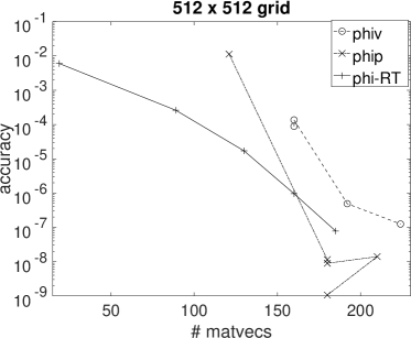
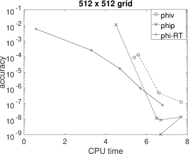
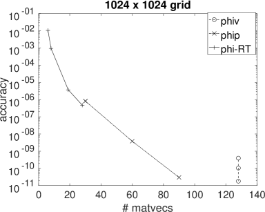
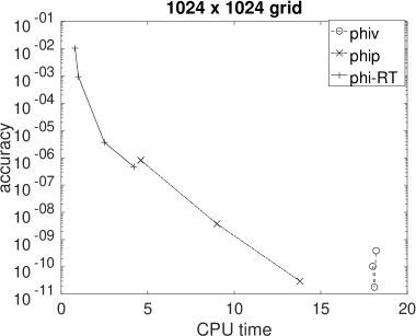
Figure 11: The finite-element discretized convection-dominated convection–diffusion test problem. Relative error versus number of the matrix-vector products (left) and versus the CPU time (right) for phiv (dashed line), phip (dash-dotted line) and phiRT (solid line). The restart length is 30 for all the three solvers. Perturbing requested tolerance from 6e-05 to 7e-05 for phip yields a change in delivered accuracy from 1.15e-08 to 1.13e-02, see the two upper left points of the dash-dotted line in the upper plots, $512\times 512$ grid. A similar effect is observed for $1024\times 1024$ grid.

Table 4: Results for the finite-element discretized convection-dominated convection–diffusion test problem, $\nu=1/12800$, $1024\times 1024$ grid

method(Krylov dim.), delivered matvecs / requested tolerance error CPU time, s phiv($30$), 1e-04 1.81e-11 128 / 18.1 phiv($30$), 1e-06 3.95e-10 128 / 18.2 phip($30$), 1e-04 5.36e-01 1 / 0.4 phip($30$), 1e-05 3.80e-09 60 / 9.0 phip($30$), 1e-06 2.99e-11 90 / 13.8 phiRT($30$), 1e-05 1.06e-02 6 / 0.8 phiRT($30$), 1e-06 9.39e-04 8 / 1.0 phiRT($30$), 1e-08 3.70e-06 19 / 2.5 phiRT($30$), 1e-09 4.72e-07 28 / 4.2 phiv($10$), 1e-05 3.54e-04 60 / 5.2 phiv($10$), 1e-06 8.86e-06 96 / 8.2 phip($10$), 1e-04 5.36e-01 1 / 0.3 phip($10$), 1e-05 1.39e-08 100 / 9.9 phiRT($10$), 1e-05 1.06e-02 6 / 0.7 phiRT($10$), 1e-06 9.39e-04 8 / 0.9 phiRT($10$), 1e-07 3.96e-05 45 / 4.4

7 Conclusions

We have proposed a Krylov subspace method for computing matrix-vector products with the $\varphi$ matrix function. It is based on the residual notion (7), which is essentially used in our algorithm both as a stopping criterion and for efficient restarting. Our analysis provides true upper bounds for the residual, with no asymptotic estimates, and shows convergence of the restarted method for an arbitrary final time interval $[0,t]$, $t<\infty$, and for any restart length (i.e., Krylov subspace dimension).

Since the residual can be seen as the backward error, the residual based stopping criterion and residual-time (RT) restarting provide a reliable error control. This is confirmed by the performance of the method: in all the test runs it either outperforms the phiv and phip solvers or delivers a comparable efficiency. More importantly, in all the test runs our method appears to deliver a monotone dependence of the obtained accuracy on the required tolerance. The phiv and phip solvers have in some cases difficulties with delivering error in the desired moderate PDE tolerance range $[10^{-7},10^{-3}]$; they tend to produce more accurate and more expensive results than requested.

Thus, the presented residual based Krylov subspace method for evaluating matrix-vector products with the $\varphi$ matrix function appears to be a promising approach useful in practical computations.

References

- [1] M. Abramowitz and I. A. Stegun, Handbook of mathematical functions with formulas, graphs, and mathematical tables, vol. 55 of National Bureau of Standards Applied Mathematics Series, For sale by the Superintendent of Documents, U.S. Government Printing Office, Washington, D.C., 1964.
- [2] M. Afanasjew, M. Eiermann, O. G. Ernst, and S. Güttel, Implementation of a restarted Krylov subspace method for the evaluation of matrix functions, Linear Algebra Appl., 429 (2008), pp. 2293–2314.
- [3] A. H. Al-Mohy and N. J. Higham, A new scaling and squaring algorithm for the matrix exponential, SIAM Journal on Matrix Analysis and Applications, 31 (2010), pp. 970–989, https://doi.org/10.1137/09074721X.
- [4] A. H. Al-Mohy and N. J. Higham, Computing the action of the matrix exponential, with an application to exponential integrators, SIAM J. Sci. Comput., 33 (2011), pp. 488–511. http://dx.doi.org/10.1137/100788860.
- [5] B. Beckermann, Image numérique, GMRES et polynômes de Faber, C. R. Acad. Sci. Paris: Ser. I, 340 (2005), pp. 855–860.
- [6] B. Beckermann and L. Reichel, Error estimation and evaluation of matrix functions via the Faber transform, SIAM J. Num. Anal., 47 (2009), pp. 3849–3883.
- [7] H. Berland, B. Skaflestad, and W. M. Wright, EXPINT—a MATLAB package for exponential integrators, ACM Trans. Math. Softw., 33 (2007). http://www.math.ntnu.no/num/expint/.
- [8] M. Botchev, I. Faragó, and R. Horváth, Application of operator splitting to the Maxwell equations including a source term, Applied Numerical Mathematics, 59 (2009), pp. 522–541, https://doi.org/DOI:10.1016/j.apnum.2008.03.031, http://dx.doi.org/10.1016/j.apnum.2008.03.031.
- [9] M. A. Botchev, Krylov subspace exponential time domain solution of Maxwell’s equations in photonic crystal modeling, J. Comput. Appl. Math., 293 (2016), pp. 24–30. http://dx.doi.org/10.1016/j.cam.2015.04.022.
- [10] M. A. Botchev, V. Grimm, and M. Hochbruck, Residual, restarting and Richardson iteration for the matrix exponential, SIAM J. Sci. Comput., 35 (2013), pp. A1376–A1397. http://dx.doi.org/10.1137/110820191.
- [11] M. A. Botchev, A. M. Hanse, and R. Uppu, Exponential Krylov time integration for modeling multi-frequency optical response with monochromatic sources, Journal of Computational and Applied Mathematics, 340 (2018), pp. 474–485. https://doi.org/10.1016/j.cam.2017.12.014.
- [12] M. A. Botchev, D. Harutyunyan, and J. J. W. van der Vegt, The Gautschi time stepping scheme for edge finite element discretizations of the Maxwell equations, J. Comput. Phys., 216 (2006), pp. 654–686. http://dx.doi.org/10.1016/j.jcp.2006.01.014.
- [13] M. A. Botchev and L. A. Knizhnerman, ART: Adaptive residual-time restarting for Krylov subspace matrix exponential evaluations, J. Comput. Appl. Math., 364 (2020), p. 112311. https://doi.org/10.1016/j.cam.2019.06.027.
- [14] M. A. Botchev and L. A. Knizhnerman, ART: Adaptive residual-time restarting for Krylov subspace matrix exponential evaluations, J. Comput. Appl. Math., 364 (2020). https://doi.org/10.1016/j.cam.2019.06.027.
- [15] M. A. Botchev, G. L. G. Sleijpen, and H. A. van der Vorst, Stability control for approximate implicit time stepping schemes with minimum residual iterations, Appl. Numer. Math., 31 (1999), pp. 239–253.
- [16] G. D. Byrne, A. C. Hindmarsh, and P. N. Brown, VODPK, large non-stiff or stiff ordinary differential equation initial-value problem solver. Available at URL www.netlib.org, 1997.
- [17] M. Caliari and A. Ostermann, Implementation of exponential Rosenbrock-type integrators, Appl. Numer. Math., 59 (2009), pp. 568–581, https://doi.org/10.1016/j.apnum.2008.03.021.
- [18] E. Celledoni and I. Moret, A Krylov projection method for systems of ODEs, Appl. Numer. Math., 24 (1997), pp. 365–378, https://doi.org/10.1016/S0168-9274(97)00033-0.
- [19] J. Certaine, The solution of ordinary differential equations with large time constants, in Mathematical Methods for Digital Computers, K. E. A. Ralston, H.S. Wilf, ed., Wiley, New York, 1960, pp. 128–132.
- [20] T. F. Chan and K. R. Jackson, The use of iterative linear-equation solvers in codes for large systems of stiff IVPs for ODEs, SIAM J. Sci. Stat. Comput., 7 (1986), pp. 378–417.
- [21] H. De Raedt, K. Michielsen, J. S. Kole, and M. T. Figge, One-step finite-difference time-domain algorithm to solve the Maxwell equations, Phys. Rev. E, 67 (2003), p. 056706.
- [22] V. L. Druskin, A. Greenbaum, and L. A. Knizhnerman, Using nonorthogonal Lanczos vectors in the computation of matrix functions, SIAM J. Sci. Comput., 19 (1998), pp. 38–54, https://doi.org/10.1137/S1064827596303661.
- [23] V. L. Druskin and L. A. Knizhnerman, Two polynomial methods of calculating functions of symmetric matrices, U.S.S.R. Comput. Maths. Math. Phys., 29 (1989), pp. 112–121.
- [24] V. L. Druskin and L. A. Knizhnerman, Krylov subspace approximations of eigenpairs and matrix functions in exact and computer arithmetic, Numer. Lin. Alg. Appl., 2 (1995), pp. 205–217.
- [25] M. Eiermann and O. G. Ernst, A restarted Krylov subspace method for the evaluation of matrix functions, SIAM Journal on Numerical Analysis, 44 (2006), pp. 2481–2504.
- [26] M. Eiermann, O. G. Ernst, and S. Güttel, Deflated restarting for matrix functions, SIAM J. Matrix Anal. Appl., 32 (2011), pp. 621–641.
- [27] M. Eiermann, O. G. Ernst, and S. Güttel, Deflated restarting for matrix functions, SIAM J. Matrix Anal. Appl., 32 (2011), pp. 621–641.
- [28] H. C. Elman, A. Ramage, and D. J. Silvester, IFISS: A computational laboratory for investigating incompressible flow problems, SIAM Review, 56 (2014), pp. 261–273.
- [29] R. P. Fedorenko, Stiff systems of ordinary differential equations, in Numerical methods and applications, CRC, Boca Raton, FL, 1994, pp. 117–154.
- [30] X. Fu, C. Wang, P. Li, and L. Wang, Exponential integration algorithm for large-scale wind farm simulation with Krylov subspace acceleration, Applied Energy, 254 (2019), p. 113692. https://doi.org/10.1016/j.apenergy.2019.113692.
- [31] E. Gallopoulos and Y. Saad, Efficient solution of parabolic equations by Krylov approximation methods, SIAM J. Sci. Statist. Comput., 13 (1992), pp. 1236–1264. http://dx.doi.org/10.1137/0913071.
- [32] S. Gaudreault, G. Rainwater, and M. Tokman, KIOPS: A fast adaptive Krylov subspace solver for exponential integrators, Journal of Computational Physics, 372 (2018), pp. 236–255. https://doi.org/10.1016/j.jcp.2018.06.026.
- [33] C. W. Gear and Y. Saad, Iterative solution of linear equations in ODE codes, SIAM J. Sci. Stat. Comput., 4 (1983), pp. 583–601.
- [34] G. H. Golub and C. F. Van Loan, Matrix Computations, The Johns Hopkins University Press, Baltimore and London, third ed., 1996.
- [35] S. Güttel, A. Frommer, and M. Schweitzer., Efficient and stable Arnoldi restarts for matrix functions based on quadrature, SIAM J. Matrix Anal. Appl, 35 (2014), pp. 661–683.
- [36] E. Hansen and A. Ostermann, High-order splitting schemes for semilinear evolution equations, BIT Numerical Mathematics, 56 (2016), pp. 1303–1316.
- [37] N. J. Higham, Functions of Matrices: Theory and Computation, Society for Industrial and Applied Mathematics, Philadelphia, PA, USA, 2008.
- [38] N. J. Higham and A. H. Al-Mohy, Computing matrix functions, Acta Numer., 19 (2010), pp. 159–208, https://doi.org/10.1017/S0962492910000036.
- [39] M. Hochbruck and C. Lubich, On Krylov subspace approximations to the matrix exponential operator, SIAM J. Numer. Anal., 34 (1997), pp. 1911–1925.
- [40] M. Hochbruck, C. Lubich, and H. Selhofer, Exponential integrators for large systems of differential equations, SIAM J. Sci. Comput., 19 (1998), pp. 1552–1574.
- [41] M. Hochbruck and A. Ostermann, Exponential integrators, Acta Numer., 19 (2010), pp. 209–286, https://doi.org/10.1017/S0962492910000048.
- [42] M. Hochbruck, A. Ostermann, and J. Schweitzer, Exponential Rosenbrock-type methods, SIAM J. Numer. Anal., 47 (2008/09), pp. 786–803, https://doi.org/10.1137/080717717. http://dx.doi.org/10.1137/080717717.
- [43] M. Hochbruck, T. Pažur, A. Schulz, E. Thawinan, and C. Wieners, Efficient time integration for discontinuous Galerkin approximations of linear wave equations, ZAMM, 95 (2015), pp. 237–259, http://dx.doi.org/10.1002/zamm.201300306.
- [44] R. A. Horn and C. R. Johnson, Matrix Analysis, Cambridge University Press, 1986.
- [45] W. Hundsdorfer and J. G. Verwer, Numerical Solution of Time-Dependent Advection-Diffusion-Reaction Equations, Springer Verlag, 2003.
- [46] L. A. Knizhnerman, Calculation of functions of unsymmetric matrices using Arnoldi’s method, U.S.S.R. Comput. Maths. Math. Phys., 31 (1991), pp. 1–9.
- [47] L. A. Krukier, Implicit difference schemes and an iterative method for solving them for a certain class of systems of quasi-linear equations, Sov. Math., 23 (1979), pp. 43–55. Translation from Izv. Vyssh. Uchebn. Zaved., Mat. 1979, No. 7(206), 41–52 (1979).
- [48] J. D. Lawson, Generalized Runge-Kutta processes for stable systems with large Lipschitz constants, SIAM J. Numer. Anal., 4 (1967), pp. 372–380.
- [49] J. Legras, Résolution numérique des grands systèmes différentiels linéaires, Numer. Math., 8 (1966), pp. 14–28.
- [50] C. B. Moler and C. F. Van Loan, Nineteen dubious ways to compute the exponential of a matrix, twenty-five years later, SIAM Rev., 45 (2003), pp. 3–49.
- [51] I. Nȧsell, Inequalities for modified Bessel functions, Math. Comp., 28 (1974), pp. 253–256. https://doi.org/10.2307/2005831.
- [52] J. Niehoff, Projektionsverfahren zur Approximation von Matrixfunktionen mit Anwendungen auf die Implementierung exponentieller Integratoren, PhD thesis, Mathematisch-Naturwissenschaftlichen Fakultät der Heinrich-Heine-Universität Düsseldorf, December 2006.
- [53] J. Niesen and W. M. Wright, Algorithm 919: A Krylov subspace algorithm for evaluating the -functions appearing in exponential integrators, ACM Trans. Math. Softw., 38 (2012), pp. 22:1–22:19, https://doi.org/10.1145/2168773.2168781.
- [54] T. J. Park and J. C. Light, Unitary quantum time evolution by iterative Lanczos reduction, J. Chem. Phys., 85 (1986), pp. 5870–5876.
- [55] B. N. Parlett, The Symmetric Eigenvalue Problem, SIAM, 1998.
- [56] S. Paszkowski, Computational Applications of Chebyshev Polynomials and Series, Nauka, 1983. Russian, translated from Polish.
- [57] Y. Saad, Analysis of some Krylov subspace approximations to the matrix exponential operator, SIAM J. Numer. Anal., 29 (1992), pp. 209–228.
- [58] Y. Saad, Iterative Methods for Sparse Linear Systems, SIAM, 2d ed., 2003. Available from http://www-users.cs.umn.edu/~saad/books.html.
- [59] T. Schmelzer and L. N. Trefethen, Evaluating matrix functions for exponential integrators via Carathéodory-Fejér approximation and contour integrals, Electron. Trans. Numer. Anal., 29 (2007/08), pp. 1–18.
- [60] R. B. Sidje, Expokit. A software package for computing matrix exponentials, ACM Trans. Math. Softw., 24 (1998), pp. 130–156. www.maths.uq.edu.au/expokit/.
- [61] D. J. Silvester, H. C. Elman, and A. Ramage, Algorithm 886: IFISS, a Matlab toolbox for modelling incompressible flow, ACM Transactions on Mathematical Software, 33 (2007).
- [62] D. J. Silvester, H. C. Elman, and A. Ramage, Incompressible flow & iterative solver software. http://www.manchester.ac.uk/ifiss/, 2019.
- [63] P. K. Suetin, Series of Faber Polynomials, CRC Press, 1998.
- [64] H. Tal-Ezer, Spectral methods in time for parabolic problems, SIAM J. Numer. Anal., 26 (1989), pp. 1–11.
- [65] H. A. van der Vorst, An iterative solution method for solving , using Krylov subspace information obtained for the symmetric positive definite matrix , J. Comput. Appl. Math., 18 (1987), pp. 249–263.
- [66] H. A. van der Vorst, BiCGSTAB: a fast and smoothly converging variant of BiCG for the solution of nonsymmetric linear systems, SIAM J. Sci. Stat. Comput., 13 (1992), pp. 631–644.
- [67] H. A. van der Vorst, Iterative Krylov methods for large linear systems, Cambridge University Press, 2003.
- [68] R. W. C. P. Verstappen and A. E. P. Veldman, Symmetry-preserving discretization of turbulent flow, J. Comput. Phys., 187 (2003), pp. 343–368. http://dx.doi.org/10.1016/S0021-9991(03)00126-8.
- [69] X. Wang, P. Chen, and C. Cheng, Stability and convergency exploration of matrix exponential integration on power delivery network transient simulation, IEEE Transactions on Computer-Aided Design of Integrated Circuits and Systems, (2019), pp. 1–1. https://doi.org/10.1109/TCAD.2019.2954473.
- [70] H. Zhuang, X. Wang, Q. Chen, P. Chen, and C. Cheng, From circuit theory, simulation to SPICEDiego: A matrix exponential approach for time-domain analysis of large-scale circuits, IEEE Circuits and Systems Magazine, 16 (2016), pp. 16–34.