Bound entanglement from randomized measurements

Abstract

If only limited control over a multiparticle quantum system is available, a viable method to characterize correlations is to perform random measurements and consider the moments of the resulting probability distribution. We present systematic methods to analyze the different forms of entanglement with these moments in an optimized manner. First, we find the optimal criteria for different forms of multiparticle entanglement in three-qubit systems using the second moments of randomized measurements. Second, we present the optimal inequalities if entanglement in a bipartition of a multi-qubit system shall be analyzed in terms of these moments. Finally, for higher-dimensional two-particle systems and higher moments, we provide criteria that are able to characterize various examples of bound entangled states, showing that detection of such states is possible in this framework.

Introduction.— With the current development of experimental quantum technologies, larger quantum systems with more and more particles become available, but controlling and analyzing these systems is complicated. In fact, due to the exponentially increasing dimension of the underlying Hilbert space, a complete characterization of the quantum states or quantum dynamics is quickly out of reach. A key idea for analyzing large quantum systems is therefore to perform random measurements or operations, and to characterize the global quantum system with the help of the observed statistics. Examples are procedures like randomized benchmarking for the analysis of quantum gates [1, 2], certain methods for estimating the fidelity of quantum states [3], or various proposals to perform variants of state tomography using random measurements [4, 5, 6, 7].

It was noted early that randomized measurements could also be used to study quantum correlations [8, 9, 10]. The original motivation came from the situation where two parties, typically called Alice and Bob, share a quantum state, but no common reference frame. This situation has been discussed in a variety of settings in quantum information processing [11, 12, 13, 14]. Although the determination of the entire quantum state is impossible in this setting, it may still be analyzed along the following lines. Alice and Bob perform separate measurements, denoted by $M_{A}$ and $M_{B}$, and rotate them arbitrarily. That is, they evaluate an expression of the form

$$\langle{M_{A}\otimes M_{B}}\rangle_{U_{A}\otimes U_{B}}=\mathrm{tr}[\varrho_{AB}(U_{A}M_{A}U_{A}^{\dagger})\otimes(U_{B}M_{B}U_{B}^{\dagger})],$$ (1)

which, of course, depends on the chosen unitary ${U_{A}\otimes U_{B}}$. The prime idea is to sample random unitaries and consider the resulting probability distribution of $\langle{M_{A}\otimes M_{B}}\rangle_{U_{A}\otimes U_{B}}$. This probability distribution contains valuable information about the state, and the distribution may be characterized by its moments

$$\mathcal{R}^{(r)}_{AB}=\int dU_{A}\int dU_{B}[\langle{M_{A}\otimes M_{B}}\rangle_{U_{A}\otimes U_{B}}]^{r},$$ (2)

where the unitaries are typically chosen according to the Haar distribution. Clearly, similar moments can be defined for multiparticle systems.

In recent years, several works proceeded in this direction. One research line has been started from the estimation of the state’s purity [15], and then protocols for measuring entanglement via Rényi entropies have been presented [16] and experimentally implemented [17]. Very recently, ideas to estimate the entanglement criterion of the positivity of the partial transpose (PPT) [18, 19] have been introduced [20, 21]. Another research line characterized the relation of the second moments [22, 23] $\mathcal{R}^{(2)}_{AB}$ and those of the marginals [24] to entanglement. Recently, higher moments have been used to characterize multiparticle entanglement [25, 26], and quantum designs have been shown to allow for a simplified implementation, as the integral in Eq. (2) can be replaced by finite sums [25, 27, 28].

Still, the present results along the above research lines are incomplete in several respects. First, while many entanglement criteria have been presented, their optimality is not clear. It would be desirable to use the information obtained by randomized measurements most efficiently. Second, the known results from randomized measurements allow one to detect highly entangled states only, e.g., states which are close to pure states. For a long-range impact of the research program, however, it is vital that also weakly entangled states, e.g., the ones that cannot be detected by the PPT criterion, can be analyzed.

The goal of this paper is to generalize the existing approaches in two directions: First, we will systematically consider the moments of the measurement results when only some of the parties measure. That is, we evaluate the expressions in Eqs. (1, 2) for the special case of $M_{A}=\mathbbm{1}$ or $M_{B}=\mathbbm{1}$, and call these quantities the reduced moments $\mathcal{R}^{(r)}_{B}$ and $\mathcal{R}^{(r)}_{A}$. Note that this case effectively corresponds to discarding the measurements of Alice for $\mathcal{R}^{(r)}_{B}$ (resp., Bob for $\mathcal{R}^{(r)}_{A}$), such that the reduced moments can directly be evaluated from the data taken for measuring $\mathcal{R}^{(r)}_{AB}$. As we will show, in terms of these reduced moments, improved entanglement criteria can be designed, which are optimal in the sense that if a quantum state is not detected by them, then there is also a separable state compatible with the data.

Second, we present a systematic approach to characterize high-dimensional systems with higher moments $\mathcal{R}^{(r)}_{AB}$. We show how previously known entanglement criteria [29, 30, 31] can be formulated in terms of moments. With this, we demonstrate that bound entanglement, a weak form of entanglement that cannot be used for entanglement distillation and is not detectable by the PPT criterion, can be also characterized in a reference-frame independent manner. This shows that the approach of randomized measurements is powerful enough to characterize the rich plethora of entanglement phenomena.

Multiparticle correlations for three qubits.— For three qubits, the measurements $M_{A},M_{B}$, and $M_{C}$ may, without loss of generality, be taken as the Pauli-$Z$ matrix $\sigma_{3}$. If we consider the full or reduced second moments $\mathcal{R}^{(2)}$, the analysis is simplified by the fact that each integral over $U(2)$ in Eq. (2) can be replaced by sums over the four Pauli matrices $\sigma_{0},\sigma_{1},\sigma_{2},$ and $\sigma_{3}$. This is because the Pauli matrices form a unitary two-design, meaning that averages of polynomials of degree two or less yield identical results [32, 25].

Accordingly, the moments are directly related to the Bloch decomposition of the three-qubit state $\varrho_{ABC}$. Recall that any three-qubit state can be written as

$$\varrho_{ABC}=\frac{1}{8}\sum_{i,j,k=0}^{3}\alpha_{ijk}\sigma_{i}\otimes\sigma_{j}\otimes\sigma_{k},$$ (3)

where $\sigma_{0}=\mathbbm{1}$ denotes the identity matrix. The full and reduced second moments can simply be expressed in terms of the coefficients $\alpha_{ijk}$, and they read

$$\mathcal{R}^{(2)}_{ABC}=\frac{1}{27}\!\!\!\!\sum_{i,j,k=1}^{3}\!\!\!\!\alpha_{ijk}^{2},\;\mathcal{R}^{(2)}_{AB}=\frac{1}{9}\!\!\sum_{i,j=1}^{3}\!\!\alpha_{ij0}^{2},\;\mathcal{R}^{(2)}_{A}=\frac{1}{3}\!\!\sum_{i=1}^{3}\!\!\alpha_{i00}^{2},$$ (4)

and similarly for the reduced moments on other parts of the three-particle system.

Sums of this form have already been considered under the concept of sector lengths [33, 34, 35, 37, 36] and multiparticle concurrences [38, 39]. More precisely, the notion of sector lengths captures the magnitude of the one-, two-, and three-body correlations in the state $\varrho_{ABC}$, where the one- and two-body correlations are averaged over all one- and two-particle reduced states. That is, the sector lengths $A_{k}$ are given by $A_{1}=3(\mathcal{R}^{(2)}_{A}+\mathcal{R}^{(2)}_{B}+\mathcal{R}^{(2)}_{C})$, $A_{2}=9(\mathcal{R}^{(2)}_{AB}+\mathcal{R}^{(2)}_{AC}+\mathcal{R}^{(2)}_{BC})$, and $A_{3}=27\mathcal{R}^{(2)}_{ABC}$. Most importantly, the set of all three-qubit states forms a polytope in the space of the sector lengths, which has recently been fully characterized [36], see also Fig. 1.

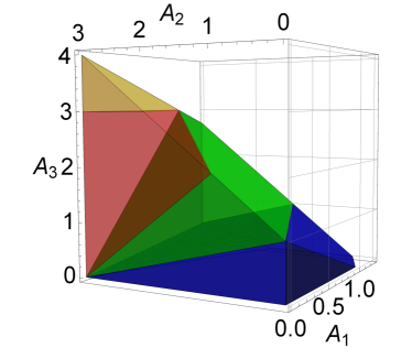
Figure 1: Geometry of the three-qubit state space in terms of the second moments of random measurements or sector lengths. The total polytope is the set of all states, characterized by the inequalities $A_{k}\geq 0$, $A_{1}-A_{2}+A_{3}\leq 1$, $A_{2}\leq 3$, and $A_{1}+A_{2}\leq 3(1+A_{3})$ [36]. The fully separable states are contained in the blue polytope, obeying the additional constraint in Eq. (6) in Observation 1. States that are biseparable for some partitions are contained in the union of the green and blue polytopes, characterized by the additional constraint in Eq. (7) from Observation 2. In fact, for any point in the green and blue areas, there is a biseparable state with the corresponding second moments. The yellow area corresponds to the states violating the best previously known criterion for biseparable states, $A_{3}\leq 3$ [33, 34, 35, 36]. Thus, the red area marks the improvement of the criterion in Observation 2 compared with previous results.

To proceed, recall that a state is fully separable if it can be written as

$$\varrho_{\text{fs}}=\sum_{k}p_{k}\varrho^{A}_{k}\otimes\varrho^{B}_{k}\otimes\varrho^{C}_{k},$$ (5)

where the $p_{k}$ form a probability distribution. Now, we can formulate the first main result of this paper.

Observation 1. Any fully separable three-qubit state obeys

$$A_{2}+3A_{3}\leq 3+A_{1}$$ (6)

or, equivalently, $3(\mathcal{R}^{(2)}_{AB}+\mathcal{R}^{(2)}_{AC}+\mathcal{R}^{(2)}_{BC})+27\mathcal{R}^{(2)}_{ABC}\leq 1+\mathcal{R}^{(2)}_{A}+\mathcal{R}^{(2)}_{B}+\mathcal{R}^{(2)}_{C}$. This is the optimal linear criterion in the sense that any other linear criterion for the $A_{i}$ detects strictly fewer states.

The proof of this Observation, including possible generalizations to higher-dimensional systems, is given in Appendix A in the Supplemental Material (SM) [40], and the geometrical interpretation is displayed in Fig. 1.

Violation of Eq. (6) implies that the state contains some entanglement, but it does not mean that all three particles are entangled. Indeed, an entangled state may still be separable with respect to some bipartition. For instance, if we consider the bipartition $A|BC$, a state separable with respect to this bipartition can be written as $\varrho_{{A|BC}}=\sum_{k}q^{A}_{k}\varrho^{A}_{k}\otimes\varrho^{BC}_{k},$ where the $q^{A}_{k}$ form a probability distribution and $\varrho^{BC}_{k}$ may be entangled. Similarly, one can define biseparable states with respect to the two other bipartitions as $\varrho_{{B|AC}}$ and $\varrho_{{C|AB}}$. For these states, we can formulate:

Observation 2. Any three-qubit state which is separable with respect to some bipartition obeys

$$A_{2}+A_{3}\leq 3(1+A_{1})$$ (7)

or, equivalently, $3(\mathcal{R}^{(2)}_{AB}+\mathcal{R}^{(2)}_{AC}+\mathcal{R}^{(2)}_{BC})+9\mathcal{R}^{(2)}_{ABC}\leq 1+3(\mathcal{R}^{(2)}_{A}+\mathcal{R}^{(2)}_{B}+\mathcal{R}^{(2)}_{C})$. This is the optimal criterion in the sense that if the three $A_{i}$ obey the inequality, then for any bipartition there is a separable state compatible with them.

Again, the proof and the generalizations to higher dimensions are given in Appendix A [40], and the geometry is displayed in Fig. 1. We add that we have strong numerical evidence that Eq. (7) also holds for mixtures of biseparable states with respect to different partitions, i.e., states of the form $\varrho_{\text{bs}}=p_{A}\varrho_{A|BC}+p_{B}\varrho_{B|AC}+p_{C}\varrho_{C|AB},$ where the $p_{A}$, $p_{B}$, and $p_{C}$ form convex weights. Nevertheless, we leave this as a conjecture for further study. More detailed information on the numerical methods used can be found in Appendix D [40].

Our two observations show that not only the three-body second moment $\mathcal{R}^{(2)}_{ABC}$, but also the one- and two-body reduced moments such as $\mathcal{R}^{(2)}_{AB}$ and $\mathcal{R}^{(2)}_{A}$ can be useful for entanglement detection. In fact, their linear combinations allow to detect entangled states more efficiently than existing criteria [33, 34, 35, 36], see also Appendix A [40].

In particular, as shown in the Appendix, Eq. (7) can detect multipartite entanglement for mixtures of Greenberger-Horne-Zeilinger (GHZ) states and W states (i.e., $\ket{\text{GHZ}}=\frac{1}{\sqrt{2}}(\ket{000}+\ket{111})$, $\ket{\text{W}}=\frac{1}{\sqrt{3}}(\ket{001}+\ket{010}+\ket{100})$, even if two other important entanglement measures, namely the three-tangle and bipartite entanglement in the reduced subsystems vanish simultaneously [62].

Optimal criteria for general bipartitions.— In many realistic scenarios, it is sufficient to detect entanglement across some fixed bipartition $I|\bar{I}$ of the multiparticle system. For this task, second moments of randomized measurements can be used as well: Performing random measurements at each qubit and considering the second moments allows one to generalize the moments in Eq. (4) for the given number of qubits. In turn, these moments allow one to determine the quantities ${\mathrm{tr}}(\varrho_{I}^{2})$, ${\mathrm{tr}}(\varrho_{\bar{I}}^{2})$, and ${\mathrm{tr}}(\varrho^{2})$ for the reduced states of the bipartition and the global state. This approach has recently been used in an experiment [17], where entanglement criteria with the second-order Rényi entropy $S_{2}(\varrho_{X})=-\log_{2}{{\mathrm{tr}}(\varrho_{X}^{2})}$ were employed. The entropic criteria for separable states read $S_{2}(\varrho_{X})\leq S_{2}(\varrho)$ for $X=I,\bar{I}$; if this is violated, then $\varrho$ is entangled [63, 64, 16].

Using our methods, we can show that this approach is optimal. To formulate the result, we assume that both sides of the bipartition have the same number of qubits. Then, recall that any bipartite state can be written as

$$\varrho_{AB}=\frac{1}{d^{2}}\sum_{i,j=0}^{d^{2}-1}t_{ij}\lambda_{i}\otimes\lambda_{j},$$ (8)

where $\lambda_{0}=\mathbbm{1}$ denotes the identity matrix and $\lambda_{i}$ are the Gell-Mann matrices [65, 66]. This is the decomposition of $\varrho_{AB}$ using the basis of Hermitian, orthogonal, and traceless matrices, i.e., $\lambda_{i}=\lambda_{i}^{\dagger}$, $\mathrm{tr}\left[\lambda_{i}\lambda_{j}\right]=d\delta_{ij}$, and $\mathrm{tr}\left[\lambda_{i}\right]=0$ for $i>0$. These properties are the natural extensions of Pauli matrices for $SU(2)$ to $SU(d)$, which are used in particle physics [67]. The quantities of interest are

$$A_{2} =\sum_{i,j=1}^{d^{2}-1}t_{ij}^{2},\;\;A_{1}^{A}=\sum_{i=1}^{d^{2}-1}t_{i0}^{2},\;\;A_{1}^{B}=\sum_{i=1}^{d^{2}-1}t_{0i}^{2}.$$ (9)

We also define $A_{1}=A_{1}^{A}+A_{1}^{B}$, which allows to recover the purities via ${\mathrm{tr}}(\varrho_{AB}^{2})=(1+A_{1}+A_{2})/d^{2}$ and ${\mathrm{tr}}({\varrho_{A}^{2}})=(1+A_{1}^{A})/d.$ It is interesting that, although the $\lambda_{i}$ are not directly linked to a quantum design, the quantities $A_{1}^{A},A_{1}^{B}$ and $A_{2}$ are also second moments of a measurement of the observables $\lambda_{i}$ in random bases. The proof follows from a slight extension of the arguments given in Ref. [23], see Appendix B [40]. This opens another possibility for an experimental implementation besides making randomized Pauli measurements on all the qubits individually. Now, we can formulate:

Observation 3. Any two-qudit separable state obeys the relation

$$A_{2}\leq d-1+{(d-1)}A_{1}^{A}-A_{1}^{B},$$ (10)

as well as the analogous one with parties $A$ and $B$ exchanged. This is equivalent to the criterion $S_{2}(\varrho_{X})\leq S_{2}(\varrho_{AB})$ for $X\in\{A,B\}$. This criterion is optimal, in the sense that if the inequality holds for $A_{1}^{A},A_{1}^{B}$ and $A_{2}$, then there is a separable state compatible with these values.

The criterion itself was established before, so we only have to prove the optimality statement. This is done in Appendix A [40], where we explicitly construct the polytope of all admissible values of $A_{1}^{A},A_{1}^{B}$ and $A_{2}$ for general and separable states in any dimension. The unfortunate consequence of the optimality statement is that any PPT entanglement cannot be detected by the quantities $A_{1}^{A},A_{1}^{B}$ and $A_{2}$ as the entropic criterion is strictly weaker than the PPT criterion [68]. In the following, we will overcome this obstacle by developing a general criterion for entanglement using higher moments of randomized measurements.

Higher-dimensional systems.— In higher-dimensional systems, different forms of entanglement exist e.g., entanglement of different dimensionality [69, 70] or bound entanglement [71, 72, 73, 74]. The previously known criteria for randomized measurements face serious problems in this scenario. First, criteria using purities, such as Observation 3, can only characterize states that violate the PPT criterion and hence miss the bound entanglement. Second, while the notion of randomized measurements as defined in Eqs. (1, 2) is independent of the dimension, many results for qubits employ the concept of a Bloch sphere, which is not available for higher dimensions, where not all observables are equivalent under randomized unitaries. Ref. [23] showed that some results for qubits are also valid for higher dimensions as long as only second moments are considered, but these connections are definitely not valid for higher moments.

To overcome these problems, we first note that a general observable is characterized by its eigenvectors, determining the probabilities of the outcomes, and the eigenvalues, corresponding to the observed values. For computing the moments as in Eq. (2), the eigenvectors do not matter due to the averaging over all unitaries. The eigenvalues are relevant, but they may be altered in classical postprocessing: Once the frequencies of the outcomes are recorded, one can calculate the moments in Eq. (2) for different assignments of values to the outcomes.

So the question arises, whether one can choose the eigenvalues of an observable in a way, such that the moments in Eq. (2) are easily tractable. For instance, it would be desirable to write them as averages over a high-dimensional sphere (the so-called pseudo-Bloch sphere). The reason is that several entanglement criteria, such as the computable cross norm or realignment criterion [29, 30] and the de Vicente (dV) criterion [31], make also use of a pseudo Bloch sphere [75]. Surprisingly, the desired eigenvalues can always be found:

Observation 4. Consider an arbitrary observable in a higher-dimensional system. Then, one can change its eigenvalues such that for the resulting observable $M_{d}$ the second and fourth moments $\mathcal{R}^{(r)}_{AB}$ in the sense of Eq. (2) equal, up to a factor, a moment $\mathcal{S}^{(r)}_{AB}$ which is taken by an integral over a generalized pseudo Bloch sphere. That is, $\mathcal{S}^{(r)}_{AB}$ is given by

$$\mathcal{S}^{(r)}_{AB}=N\int d\bm{\alpha}_{1}\int d\bm{\alpha}_{2}[\mathrm{tr}(\varrho_{AB}\bm{\alpha}_{1}\cdot\bm{\lambda}\otimes\bm{\alpha}_{2}\cdot\bm{\lambda})]^{r},$$ (11)

where $\bm{\alpha}_{i}$ denote $(d^{2}-1)$-dimensional unit real vectors uniformly distributed from the pseudo Bloch sphere, and $\bm{\lambda}=(\lambda_{1},\lambda_{2},\ldots,\lambda_{d^{2}-1})$ is the vector of Gell-Mann matrices. Furthermore, $N$ is a normalization factor.

The proof and the detailed form of $M_{d}$ are given in Appendix B [40]. To give a simple example, for $d=3$ one may measure the standard spin measurement $J_{z}$ and assign the values $\alpha_{+}/\gamma$, $\alpha_{-}/\gamma$ and $2\beta/\gamma$ instead of the standard values $\pm 1$ and $0$ to the three possible outcomes, where $\alpha_{\pm}=\pm 3-\beta$, $\beta=-\sqrt{7+2\sqrt{15}}$, and $\gamma={2\sqrt{5+\sqrt{15}}}.$ Note that the resulting observable is also traceless.

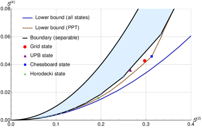
Figure 2: Entanglement criterion based on second and fourth moments of randomized measurements for $3\otimes 3$ systems. Separable states are contained in the light-blue area, according to the discussion in the main text. Several bound entangled states (denoted by colored symbols) are outside, meaning that their entanglement can be detected with the methods developed in this paper. For comparison, we also indicate a lower bound on the fourth moment for PPT states, obtained by numerical optimization, as well as a bound for general states. Further details, such as the form of the states, are given in Appendix C. Information on the numerical methods is found in Appendix D [40].

It remains to formulate separability criteria in terms of the second and fourth moments $\mathcal{S}^{(r)}_{AB}$. For that, we employ the dV criterion [31], details of the calculations are given in Appendix B [40]. From these results, it also follows that the dV criterion can be evaluated via randomized measurements for all dimensions. First, it turns out that $\mathcal{S}^{(2)}_{AB}$ and $\mathcal{S}^{(4)}_{AB}$ can, for any dimension, be simply expressed as polynomial functions of the subset of the two-body correlation coefficients $t_{ij}$ with $1\leq i,j\leq d^{2}-1$ in Eq. (8), where we also call this submatrix $T_{\mathrm{s}}$. Second, the moments $\mathcal{S}^{(r)}_{AB}$ are by definition invariant under orthogonal transformations of the matrix $T_{\mathrm{s}}$. On the other hand, the dV criterion reads that two-qudit separable states obey $\|T_{\mathrm{s}}\|_{\text{tr}}\leq d-1$, and this is also invariant under the named orthogonal transformations. Third, for a fixed value of the second moment $\mathcal{S}^{(2)}_{AB}$, we can maximize and minimize the fourth moment $\mathcal{S}^{(4)}_{AB}$ under the constraint $\|T_{\mathrm{s}}\|_{\text{tr}}\leq d-1$. This task is greatly simplified by orthogonal invariance; in fact, we can assume $T_{\mathrm{s}}$ to be diagonal. This leads to simple, piece-wise algebraic separability conditions for arbitrary dimensions $d$.

The results for $d=3$ are shown in Fig. 2. The outlined procedure gives an area that contains all values of $\mathcal{S}^{(2)}_{AB}$ and $\mathcal{S}^{(4)}_{AB}$ for separable states. Most importantly, various bound entangled states can be detected [76, 77, 78, 79]. Also for $d=4$ bound entanglement can be detected, details are given in Appendix C [40].

Conclusion.— We have developed methods for characterizing quantum correlations using randomized measurements. On the one hand, our approach led to optimal criteria for different forms of entanglement using the second moments of the randomized measurements. On the other hand, we have shown that using fourth moments of randomized measurement detection of bound entanglement as a weak form of entanglement is possible. This opens a new perspective for developing the approach further, as all previous entanglement criteria were only suited for highly entangled states.

There are several directions for further research. First, on a more technical level, the employed separability criterion [31] can be derived from an approach towards entanglement using covariance matrices [80]. Connecting randomized measurements to this approach will automatically lead to further results, e.g., on the quantification of entanglement [81]. Second, for experimental studies of the criteria presented in this article, a scheme for the statistical analysis of finite data, e.g., using the Hoeffding inequality or other large deviation bounds, is needed. Finally, our results encourage to develop the characterization of other quantum properties using randomized measurements, such as spin squeezing or the quantum Fisher information in metrology.

Appendix A: Separability criteria with sector lengths

In Appendix A, we first explain the notion of sector lengths and known simple entanglement criteria. Second, we present a criterion of full separability and prove thereby Observation 1. Third, we propose a criterion of biseparability for fixed bipartitions and prove Observation 2. Fourth, we discuss whether Observation 2 is also valid for mixtures of biseparable states with respect to different bipartitions. We discuss numerical evidence for this conjecture and also present a proof for a special case. Fifth, we discuss the improvements of our three-qubit separability criteria, in comparison with existing criteria. Sixth, we give a detailed discussion of Observation 3 and provide a proof. Finally, we characterize two-qudit states with sector lengths and discuss the strength of the separability criterion.

A1. Sector lengths

Let $\varrho$ be a $n$-particle and $d$-dimensional quantum ($n$-qudit) state. The state $\varrho$ can be written in the generalized Bloch representation

$$\varrho=\frac{1}{d^{n}}\sum_{i_{1},\cdots,i_{n}=0}^{d^{2}-1}\alpha_{i_{1}\cdots i_{n}}\lambda_{i_{1}}\otimes\cdots\otimes\lambda_{i_{n}},$$ (S.1)

where $\lambda_{0}$ is the identity, and $\lambda_{i}$ are the Gell-Mann matrices, normalized such that $\lambda_{i}=\lambda_{i}^{\dagger}$, $\mathrm{tr}\left[\lambda_{i}\lambda_{j}\right]=d\delta_{ij}$, and $\mathrm{tr}\left[\lambda_{i}\right]=0$ for $i>0$. The real coefficients $\alpha_{i_{1}\cdots i_{n}}$ are given by $\alpha_{i_{1}\cdots i_{n}}=\mathrm{tr}\left[\varrho\lambda_{i_{1}}\otimes\cdots\otimes\lambda_{i_{n}}\right]=\Braket{\lambda_{i_{1}}\otimes\cdots\otimes\lambda_{i_{n}}}$. The state $\varrho$ can be represented by

$$\varrho=\frac{1}{d^{n}}\left(\mathbbm{1}^{\otimes n}+P_{1}+P_{2}+\cdots+P_{n}\right),$$ (S.2)

where the Hermitian operators $P_{k}$ for $k=1,2,\ldots,n$ denote the sum of all terms coming from the basis elements with weight $k$

$$P_{k}(\varrho)=\sum_{\begin{subarray}{c}i_{1},\cdots,i_{n}=0,\\ \mathrm{wt}(\lambda_{i_{1}}\otimes\cdots\otimes\lambda_{i_{n}})=k\end{subarray}}^{d^{2}-1}\alpha_{i_{1}\cdots i_{n}}\lambda_{i_{1}}\otimes\cdots\otimes\lambda_{i_{n}},$$ (S.3)

where the weight $\mathrm{wt}(\lambda_{i_{1}}\otimes\cdots\otimes\lambda_{i_{n}})$ is the number of non-identity Gell-Mann matrices. Now, we can define sector lengths as

$$A_{k}(\varrho)=\frac{1}{d^{n}}\mathrm{tr}\left[P_{k}(\varrho)^{2}\right]=\sum_{\begin{subarray}{c}i_{1},\cdots,i_{n}=0,\\ \mathrm{wt}(\lambda_{i_{1}}\otimes\cdots\otimes\lambda_{i_{n}})=k\end{subarray}}^{d^{2}-1}\alpha_{i_{1}\cdots i_{n}}^{2}.$$ (S.4)

Physically, the sector lengths $A_{k}$ quantify the amount of $k$-body quantum correlations. Note that $A_{0}=\alpha_{0\cdots 0}=1$ due to $\text{tr}(\varrho)=1$. The sector lengths $A_{k}$ can be associated with the purity of $\varrho$:

$$\mathrm{tr}(\varrho^{2})=\frac{1}{d^{n}}\sum_{i_{1},\cdots,i_{n}=0}^{d^{2}-1}\alpha_{i_{1}\cdots i_{n}}^{2}=\frac{1}{d^{n}}\sum_{k=0}^{n}A_{k}(\varrho).$$ (S.5)

As the simplest case, if we consider a single-qubit state ($n=1$ and $d=2$), it holds that $\mathrm{tr}(\varrho^{2})=(1+A_{1})/2\leq 1$, which leads to $A_{1}\leq 1$.

There are three useful properties of sector lengths. The first one is local-unitary invariance, $A_{k}(\varrho)=A_{k}\big{(}U_{1}\otimes\cdots\otimes U_{n}\varrho U_{1}^{\dagger}\otimes\cdots\otimes U_{n}^{\dagger}\big{)}$. The second one is convexity, $A_{k}\left(\sum_{i}p_{i}\ket{\psi_{i}}\!\bra{\psi_{i}}\right)\leq\sum_{i}p_{i}A_{k}(\ket{\psi_{i}})$. The third one is a convolution property: for a $n$-particle state $\varrho_{P}\otimes\varrho_{Q}$, $A_{k}(\varrho_{P}\otimes\varrho_{Q})=\sum_{i=0}^{k}A_{i}(\varrho_{P})A_{k-i}(\varrho_{Q})$, where $\varrho_{P}$ and $\varrho_{Q}$ are respectively $j$-particle and $(n-j)$-particle states. Due to these properties, the sector lengths can be useful for entanglement detection [33, 34, 35, 36].

For example, for all two-qubit separable states ($n=d=2$), it holds that

$$A_{2}\big{(}\sum_{i}p_{i}\ket{\psi_{i}^{A}}\!\bra{\psi_{i}^{A}}\otimes\ket{\psi_{i}^{B}}\!\bra{\psi_{i}^{B}}\big{)}\leq\sum_{i}p_{i}A_{2}\left(\ket{\psi_{i}^{A}}\!\bra{\psi_{i}^{A}}\otimes\ket{\psi_{i}^{B}}\!\bra{\psi_{i}^{B}}\right)=\sum_{i}p_{i}A_{1}(\ket{\psi_{i}^{A}})A_{1}(\ket{\psi_{i}^{B}})\leq\sum_{i}p_{i}=1.$$ (S.6)

Conversely, if $A_{2}>1$, then the two-qubit state is entangled. In fact, since the Bell state $\ket{{\Phi^{+}}}=(\ket{00}+\ket{11})/\sqrt{2}$ can be written as $\ket{{\Phi^{+}}}\!\bra{{\Phi^{+}}}=\left(\mathbb{I}\otimes\mathbb{I}+X\otimes X-Y\otimes Y+Z\otimes Z\right)/4$, its sector lengths are given by $(A_{1},A_{2})=(0,3)$, violating the separability criterion $A_{2}\leq 1$.

A2. Criterion of full separability and proof of Observation 1

Now we present the three-qudit generalization of the fully separability criterion (6) in Observation 1 in the main text.

Observation 5. Any fully separable three-qudit state obeys

$$A_{3}\leq d-1+\frac{2d-3}{3}A_{1}+\frac{d-3}{3}A_{2}.$$ (S.7)

Remark.

In $d=2$, one obtains Eq. (6): $A_{2}+3A_{3}\leq 3+A_{1}$, also shown in Fig. 1 in the main text. Since one can easily construct fully separable states on two of the three sides of the resulting triangle (i.e., the surface where equality holds), this criterion is optimal in the sense that any other linear criterion for the $A_{k}$ detects strictly fewer states. Extensive numerical search suggests, however, that there are points on the triangle surface plane which cannot originate from a separable state. This may indicate that there exist stronger, non-linear criteria for full separability using sector lengths. For more details on the numerical optimization, see Appendix D.

Proof.

First, recall that a three-particle state is fully separable if it can be written as

$$\varrho_{\text{fs}}=\sum_{k}p_{k}\varrho^{A}_{k}\otimes\varrho^{B}_{k}\otimes\varrho^{C}_{k}.$$ (12)

Let us consider the reduced density matrix on the subsystem $AB$: $\varrho_{AB}={\mathrm{tr}}_{C}(\varrho_{\text{fs}})=\sum_{k}p_{k}\varrho^{A}_{k}\otimes\varrho^{B}_{k}$. Then we have

$${\mathrm{tr}}(\varrho_{\text{fs}}^{2})=\sum_{k,l}p_{k}p_{l}\,\mathrm{tr}(\varrho^{A}_{k}\varrho^{A}_{l})\ \mathrm{tr}(\varrho^{B}_{k}\varrho^{B}_{l})\ \mathrm{tr}(\varrho^{C}_{k}\varrho^{C}_{l})\leq\sum_{k,l}p_{k}p_{l}\,\mathrm{tr}(\varrho^{A}_{k}\varrho^{A}_{l})\ \mathrm{tr}(\varrho^{B}_{k}\varrho^{B}_{l})={\mathrm{tr}}(\varrho_{AB}^{2}),$$ (S.9)

where $\mathrm{tr}(\varrho^{C}_{k}\varrho^{C}_{l})\leq\sqrt{\mathrm{tr}(\varrho^{C}_{k})^{2}}\sqrt{\mathrm{tr}(\varrho^{C}_{l})^{2}}\leq 1$. Similarly, we obtain ${\mathrm{tr}}(\varrho_{\text{fs}}^{2})\leq{\mathrm{tr}}(\varrho_{AC}^{2})$ and ${\mathrm{tr}}(\varrho_{\text{fs}}^{2})\leq{\mathrm{tr}}(\varrho_{BC}^{2})$. Summarizing these three purity inequalities gives

$$3{\mathrm{tr}}(\varrho_{\text{fs}}^{2})\leq{\mathrm{tr}}(\varrho_{AB}^{2})+{\mathrm{tr}}(\varrho_{AC}^{2})+{\mathrm{tr}}(\varrho_{BC}^{2}).$$ (S.10)

Then, with the help of the relation (S.5), translating this inequality to the form with sector lengths yields Eq. (S.7). ∎

A3. Criterion of biseparability and proof of Observation 2

Now we discuss the three-qudit generalization of the biseparability criterion (7) in Observation 2 in the main text.

Observation 6. Any three-qudit state which is separable with respect to some bipartition obeys

$$A_{2}+A_{3}\leq\frac{d^{3}-2}{2}(1+A_{1}).$$ (S.11)

Remark.

In $d=2$, one obtains Eq. (7): $A_{2}+A_{3}\leq 3(1+A_{1})$, as shown in Fig. 1 in the main text. This is the optimal criterion in the sense that if the three $A_{k}$ obey the inequality, then for any bipartition there is a separable state compatible with them. This can be seen as follows: Eq. (7) is saturated by a family of biseparable three-qubit states

$$\sigma=p\ket{0}\!\bra{0}\otimes\ket{\psi}\!\bra{\psi}+(1-p)\ket{1}\!\bra{1}\otimes\ket{\phi}\!\bra{\phi},$$ (S.12)

where

$$\ket{\psi}=a\ket{00}+b\ket{11},\ \ \ \ket{\phi}=c\ket{00}+d\ket{11},\ \ \ a^{2}+b^{2}=c^{2}+d^{2}=1,\ \ \ \frac{1}{2}\leq p\leq 1,$$

$$\sqrt{1-\frac{1}{2p}}\leq a\leq\sqrt{\frac{1}{2p}},\ \ \ a^{2}\leq b^{2},\ \ \ c=\sqrt{\frac{2pa^{2}-1}{2(p-1)}},\ \ \ d=\pm\sqrt{1-c^{2}}.$$ (S.13)

Since the state $\sigma$ has the sector lengths

$$A_{1} =(2p-1)^{2},$$ (S.14)

$$A_{2} =1+2[2pab+2(1-p)cd]^{2}+2[p(a^{2}-b^{2})-(1-p)(c^{2}-d^{2})]^{2},$$ (S.15)

$$A_{3} =(2p-1)^{2}+2[2pab-2(1-p)cd]^{2},$$ (S.16)

it satisfies the equality $A_{2}+A_{3}=3(1+A_{1})$ and lies on the plane displayed as the boundary between the red and green areas in the polytope in Fig. 1. In order to see that this family indeed fills the entired plane, we display the plane and states from the family in Fig. (3).

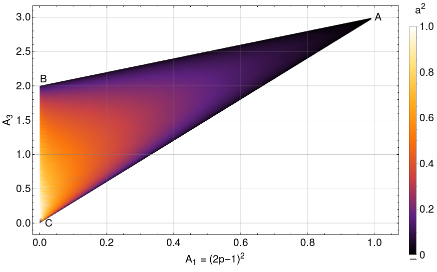
Figure 3: Location of states from the family defined in Eq. (S.12) covering the plane given by Eq. (7) in a $(A_{1}$,$A_{3}$)-plot. While the parameter $p$ fixes the $A_{1}$-coordinate via $A_{1}=(2p-1)^{2}$, the parameter $a$ together with a choice of sign for $d$ defines the $A_{3}$-coordinate. The labelled vertices correspond to the states $|0\rangle\langle 0|\otimes|\Phi^{+}\rangle\langle\Phi^{+}|$ (A), $\frac{1}{2}|0\rangle\langle 0|\otimes|\Phi^{+}\rangle\langle\Phi^{+}|+\frac{1}{2}|1\rangle\langle 1|\otimes|\Phi^{-}\rangle\langle\Phi^{-}|$ (B) and $\frac{1}{2}|0\rangle\langle 0|\otimes|\Phi^{+}\rangle\langle\Phi^{+}|+\frac{1}{2}|1\rangle\langle 1|\otimes|\Phi^{+}\rangle\langle\Phi^{+}|$ (C).

Proof.

Let $\varrho_{\text{bs}}$ be a separable three-qudit state with respect to a bipartition, and let $\varrho_{X}$ be its reduced density matrices on the subsystems $X$ for $X\in\{A,B,C\}$. With the help of the relation (S.5), we notice that Eq. (S.11) is equivalent to

$$1+\mathrm{tr}(\varrho_{\text{bs}}^{2})\leq\frac{d}{2}\left[\mathrm{tr}(\varrho_{A}^{2})+\mathrm{tr}(\varrho_{B}^{2})+\mathrm{tr}(\varrho_{C}^{2})\right].$$ (S.17)

In the following, without loss of generality, we consider a separable state with respect to a fixed bipartition $A|BC$:

$$\varrho_{{A|BC}}=\sum_{k}q_{k}\varrho^{A}_{k}\otimes\varrho^{BC}_{k}.$$ (13)

Since its reduced density matrix on the subsystem $A$ is given by $\varrho_{{A}}=\sum_{k}q_{k}\varrho^{A}_{k}$, we have

$${\mathrm{tr}}(\varrho_{{A|BC}}^{2})=\sum_{k,l}q_{k}q_{l}\,\mathrm{tr}(\varrho^{A}_{k}\varrho^{A}_{l})\ \mathrm{tr}(\varrho^{BC}_{k}\varrho^{BC}_{l})\leq\sum_{k,l}q_{k}q_{l}\,\mathrm{tr}(\varrho^{A}_{k}\varrho^{A}_{l})={\mathrm{tr}}(\varrho_{{A}}^{2}),$$ (S.19)

where $\mathrm{tr}(\varrho^{BC}_{k}\varrho^{BC}_{l})\leq 1$. In addition, it follows from the relation (S.5) for single particles

$$\mathrm{tr}(\varrho_{B}^{2})+\mathrm{tr}(\varrho_{C}^{2})=\frac{1}{d}(2+A_{1}^{B}+A_{1}^{C}),$$ (S.20)

where we split $A_{1}=A_{1}^{A}+A_{1}^{B}+A_{1}^{C}$ corresponding to the contributions from the three particles. Then we have

$$1+{\mathrm{tr}}(\varrho_{{A|BC}}^{2})-\frac{d}{2}\left[\mathrm{tr}(\varrho_{A}^{2})+\mathrm{tr}(\varrho_{B}^{2})+\mathrm{tr}(\varrho_{C}^{2})\right] \leq 1+\mathrm{tr}(\varrho_{A}^{2})-\frac{d}{2}\left[\mathrm{tr}(\varrho_{A}^{2})+\mathrm{tr}(\varrho_{B}^{2})+\mathrm{tr}(\varrho_{C}^{2})\right]$$

$$=1+\left(1-\frac{d}{2}\right){\mathrm{tr}}(\varrho_{{A}}^{2})-\frac{1}{2}(2+A_{1}^{B}+A_{1}^{C})$$

$$=\left(1-\frac{d}{2}\right){\mathrm{tr}}(\varrho_{{A}}^{2})-\frac{1}{2}(A_{1}^{B}+A_{1}^{C})\leq 0.$$

∎

A4. Evidence for the validity of Observation 2 for mixtures of different bipartitions

While Observation 6 holds true for mixed states of fixed bipartitions, we collected evidence for the conjecture that for $d=2$, the bound is also true for mixtures of different bipartitions. To that end, we numerically maximized the expression $A_{2}+A_{3}-3(1+A_{1})$ for mixtures of up to eight biseparable three-qubit states with different bipartitions and found no violation (see Appendix D for details). Furthermore, we can analytically show that mixtures of two product states for different bipartitions obey the bound as well:

Observation 7. For three-qubit systems, a rank-$2$ mixture of two pure biseparable states with respect to different partitions obeys the biseparability criterion (7) in the main text.

Proof.

Let $\varrho$ be a rank-$2$ mixture of two pure biseparable states with respect to different partitions, without loss of generality, $A|BC$ and $AB|C$:

$$\varrho=p\ket{\Psi}\!\bra{\Psi}+(1-p)\ket{\Phi}\!\bra{\Phi},$$ (S.21)

where $0\leq p\leq 1$, and without loss of generality, we can write

$$\ket{\Psi} =\ket{0}\otimes\left(\lambda_{0}\ket{00}+\lambda_{1}\ket{11}\right),\ \ \ \ \ \ 0\leq\lambda_{0},\,\lambda_{1}\leq 1,\ \ \ \ \ \ \lambda_{0}^{2}+\lambda_{1}^{2}=1,$$

$$\ket{\Phi} =\sum_{i,j=0}^{1}\kappa_{ij}\ket{ij}\otimes\left(c_{0}\ket{0}+c_{1}\ket{1}\right),\ \ \ \ \ \ \kappa_{ij},\,c_{1},\,c_{2}\in\mathbb{C},\ \ \ \ \ \ \sum_{i,j=0}^{1}|\kappa_{ij}|^{2}=|c_{0}|^{2}+|c_{1}|^{2}=1.$$ (S.22)

Now, we define a function

$$f(\varrho_{1},\varrho_{2})\equiv 1+\mathrm{tr}(\varrho_{1}\varrho_{2})-\mathrm{tr}(\varrho_{A_{1}}\varrho_{A_{2}})-\mathrm{tr}(\varrho_{B_{1}}\varrho_{B_{2}})-\mathrm{tr}(\varrho_{C_{1}}\varrho_{C_{2}}),$$ (S.23)

where $\varrho_{i}$ $(i=1,2)$ are three-particle quantum states and $\varrho_{X_{i}}$ for $X\in\{A,B,C\}$ are their reduced density matrices on the subsystems $X$. Our aim is to prove that the biseparable state $\varrho$ obeys

$$1+\mathrm{tr}(\varrho^{2})\leq\mathrm{tr}(\varrho_{A}^{2})+\mathrm{tr}(\varrho_{B}^{2})+\mathrm{tr}(\varrho_{C}^{2}).$$ (S.24)

This is equivalent to proving that the following function $F(\varrho)$ is non-positive:

$$F(\varrho) =1+\mathrm{tr}(\varrho^{2})-\mathrm{tr}(\varrho_{A}^{2})-\mathrm{tr}(\varrho_{B}^{2})-\mathrm{tr}(\varrho_{C}^{2})$$

$$=p^{2}f(\Psi,\Psi)+(1-p)^{2}f(\Phi,\Phi)+2p(1-p)f(\Psi,\Phi).$$ (S.25)

A straightforward calculations yields

$$f(\Psi,\Psi) =1-2(\lambda_{0}^{4}+\lambda_{1}^{4}),$$ (S.26)

$$f(\Phi,\Phi) =1-2\mathrm{tr}(\kappa\kappa^{\dagger}\kappa\kappa^{\dagger}),$$ (S.27)

$$f(\Psi,\Phi) =1+|\lambda_{0}\kappa_{00}c_{0}+\lambda_{1}\kappa_{01}c_{1}|^{2}-(\kappa_{00}^{2}+\kappa_{01}^{2})-\left[\lambda_{0}^{2}(\kappa_{00}^{2}+\kappa_{10}^{2})+\lambda_{1}^{2}(\kappa_{01}^{2}+\kappa_{11}^{2})\right]-\left(\lambda_{0}^{2}|c_{0}|^{2}+\lambda_{1}^{2}|c_{1}|^{2}\right),$$ (S.28)

where $\kappa=(\kappa_{ij})$. Here, since $\kappa_{ij}$ and $c_{i}$ can be taken as real, we obtain $|\lambda_{0}\kappa_{00}c_{0}+\lambda_{1}\kappa_{01}c_{1}|^{2}\leq 2\left(\lambda_{0}^{2}\kappa_{00}^{2}c_{0}^{2}+\lambda_{1}^{2}\kappa_{01}^{2}c_{1}^{2}\right)$. Also, for the $2\times 2$ matrix $\kappa$ we know that $1-2\mathrm{tr}(\kappa\kappa^{\dagger}\kappa\kappa^{\dagger})=4(\det\kappa)^{2}-1$. Thus we have

$$F(\varrho) \leq p^{2}\left[1-2(\lambda_{0}^{4}+\lambda_{1}^{4})\right]+(1-p)^{2}\left[4(\det\kappa)^{2}-1\right]$$

$$\quad+2p(1-p)\left[1+\lambda_{0}^{2}c_{0}^{2}(2\kappa_{00}^{2}-1)+\lambda_{1}^{2}c_{1}^{2}(2\kappa_{01}^{2}-1)-(\kappa_{00}^{2}+\kappa_{01}^{2})-\lambda_{0}^{2}(\kappa_{00}^{2}+\kappa_{10}^{2})-\lambda_{1}^{2}(\kappa_{01}^{2}+\kappa_{11}^{2})\right].$$ (S.29)

Now, it is sufficient to show that the maximization of the right-hand side is non-positive. In fact, the best choice is to set

$$c_{0}^{2} =1,\ \ \ \ c_{1}^{2}=0,\ \ \ \ \ \mathrm{if}\ \ (2\kappa_{01}^{2}-1)\lambda_{1}^{2}\leq(2\kappa_{00}^{2}-1)\lambda_{0}^{2},$$ (S.30)

$$c_{1}^{2} =1,\ \ \ \ c_{0}^{2}=0,\ \ \ \ \ \mathrm{if}\ \ (2\kappa_{00}^{2}-1)\lambda_{0}^{2}\leq(2\kappa_{01}^{2}-1)\lambda_{1}^{2}.$$ (S.31)

Let us consider the former case: $c_{0}^{2}=1$ and $c_{1}^{2}=0$. Due to that $\sum_{i,j}\,\kappa_{ij}^{2}=\lambda_{0}^{2}+\lambda_{1}^{2}=1$, we find

$$F(\varrho)\leq p^{2}\left\{1-2\left[\lambda_{0}^{4}+(1-\lambda_{0}^{2})^{2}\right]\right\}+(1-p)^{2}\left[4(\det\kappa)^{2}-1\right]+2p(1-p)\left(\kappa_{10}^{2}-\kappa_{01}^{2}-2\lambda_{0}^{2}\kappa_{10}^{2}\right).$$ (S.32)

Maximization of the right-hand side with respect to $\lambda_{0}^{2}$ can be achieved by three cases: (1) $\lambda_{0}^{2}=0$, (2) $\lambda_{0}^{2}=1$, (3) $\lambda_{0}^{2}=[1-(1-p)\kappa_{10}^{2}/2p]/2$ if $\kappa_{10}<{p}/({1-p})$. In all cases, we can immediately show that $F(\varrho)\leq 0$. ∎

A5. Discussion of the three-qubit separability criteria

Here, we focus on the case of qubit systems. The existing criteria are as follows. (i) any fully separable three-qubit state obeys $A_{3}\leq 1$ [34, 23]. If this inequality is violated, the state is entangled but it may be still separable for some bipartition. (ii) any biseparable three-qubit state obeys $A_{3}\leq 3$ [34, 36]. If this is violated, the state is genuinely tripartite entangled. Note that these existing criteria can straightforwardly be derived from the convexity and convolution of sector lengths. In the following, we will show that our criteria (6, 7) significantly improve the existing criteria, introducing some examples.

A good example for three-qubit states are the noisy GHZ-W mixed states [45, 46]:

$$\varrho=g\ket{\mathrm{GHZ}}\bra{\mathrm{GHZ}}+w\ket{\mathrm{W}}\bra{\mathrm{W}}+\frac{1-g-w}{8}\mathbbm{1}^{\otimes 3},$$ (14)

where $0\leq g,w\leq 1$, and the GHZ state and the W state are given by

$$\ket{\mathrm{GHZ}}=\frac{1}{\sqrt{2}}\left(\ket{000}+\ket{111}\right),\ \ \ \ \ket{\mathrm{W}}=\frac{1}{\sqrt{3}}\left(\ket{001}+\ket{010}+\ket{100}\right),$$ (15)

where $\Braket{\mathrm{GHZ}}{\mathrm{W}}=0$. The noisy GHZ-W mixed state has $(A_{1},A_{2},A_{3})=\left(w^{2}/3,3g^{2}+3w^{2}-2gw,4g^{2}+11w^{2}/3\right)$. To analyze this state, we consider three cases: (i) the noisy GHZ state, i.e., $w=0$ (ii) the noisy W state, i.e., $g=0$ (iii) the GHZ-W mixed state, i.e., $g+w=1$. Tables 1 and 2 list the results of our criteria, comparing them to the existing criteria and the optimal values. Also, the criteria for the state (14) are illustrated on the $g-w$ plane in Fig. 4.

Criteria for full separability
Three-qubit states	$A_{3}\leq 1$	Eq. (6)	Optimal values
$w=0$: noisy GHZ mixture	$g\leq 0.5$	$g\leq\frac{1}{\sqrt{5}}\approx 0.447$	$g\leq 0.2$ [48]
$g=0$: noisy W mixture	$w\leq\sqrt{\frac{3}{11}}\approx 0.522$	$w\leq\frac{3}{\sqrt{41}}\approx 0.469$	$w\leq 0.177$ [49]
$g+w=1$: GHZ-W mixture	all states detected	all states detected

Table 1: Results for the fully separable criterion in Eq. (6) in the main text, compared with the existing criterion $A_{3}\leq 1$ and the optimal values. For $w=0$ or $g=0$, the noisy mixed GHZ and W state are known to be fully separable iff $g\leq 0.2$ [48] and $w\leq 0.177$ [49]. Clearly, the bound (6) improves the existing bound $A_{3}\leq 1$.

Criteria for biseparability
Three-qubit states	$A_{3}\leq 3$	Eq. (7)	Optimal values
$w=0$: noisy GHZ mixture	$g\leq\frac{\sqrt{3}}{2}\approx 0.866$	$g\leq\sqrt{\frac{3}{7}}\approx 0.655$	$g\leq\frac{3}{7}\approx 0.429$ [50]
$g=0$: noisy W mixture	$w\leq\frac{3}{\sqrt{11}}\approx 0.905$	$w\leq\frac{3}{\sqrt{17}}\approx 0.728$	$w\leq 0.479$ [51]
$g+w=1$: GHZ-W mixture	$0.102\leq g\leq 0.855$	$0.297\leq g\leq 0.612$

Table 2: Results for the biseparable criterion Eq. (7) in the main text, compared with the existing criterion $A_{3}\leq 3$ and the optimal values. For $w=0$ or $g=0$, the noisy mixed GHZ and W state are known to be biseparable iff $g\leq 0.429$ [50] and $w\leq 0.479$ [51]. For $g+w=1$ ($w=1-g$), the existing criterion and our criterion (7), respectively, imply that the GHZ-W mixed state can be biseparable only in some interval for $g$. Interestingly, Ref. [45] has analyzed the GHZ-W mixed states using the three-tangle $\tau$ and the squared concurrences $C_{XY}^{2}$ measuring bipartite entanglement in the reduced states (note that all reduced states are equivalent). It has been shown that for a region $0.292\leq g\leq 0.627$, the state has zero three-tangle and zero concurrence in the reduced states . This region is larger than the region which is not detected by Eq. (7). Thus, Observation 2 can detect multiparticle entanglement even when the three-tangle as well as bipartite entanglement in reduced states vanishes.

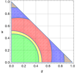
Figure 4: Entanglement criteria for the noisy GHZ-W state (14) in the $g-w$ plane. Previously, several works [47, 46] have discussed entanglement criteria in this two-parameter space. The fully separable states are contained in the green area, obeying our criterion (6). The outside of the green and yellow areas corresponds to the biseparable or genuine entangled states that violate a previously known criterion for fully separable states, $A_{3}\leq 1$. Thus, the yellow area marks the improvement of Observation 1 compared with previous results. Also, states that are biseparable for some partitions are contained in the union of the green, yellow, and red areas, characterized by our criterion (7). The brown area corresponds to the genuine entangled states violating a previously known criterion for biseparable states, $A_{3}\leq 3$. Thus, the blue area marks the improvement of Observation 2 compared with previous results.

A6. Criterion of separability and proof of Observation 3

Let us present the more general description of the separability criterion (10) in Observation 3 in the main text.

Observation 8. Any two-qudit separable state obeys the relation

$$A_{2} \leq d-1+\min\{(d-1)A_{1}^{A}-A_{1}^{B},(d-1)A_{1}^{B}-A_{1}^{A}\}.$$ (S.35)

For $A_{1}^{A}\leq A_{1}^{B}$, this relation becomes

$$A_{2}\leq d-1+{(d-1)}A_{1}^{A}-A_{1}^{B},$$ (S.36)

as well as the analogous one with parties $A$ and $B$ exchanged. This is equivalent to the criterion $S_{2}(\varrho_{X})\leq S_{2}(\varrho_{AB})$ for $X\in\{A,B\}$, where $S_{2}$ denotes the second-order Rényi entropy and $\varrho_{X}$ denote the reduced density matrices. This criterion is optimal, in the sense that if the inequality holds for $A_{1}^{A},A_{1}^{B}$ and $A_{2}$, then there is a separable state compatible with these values.

Proof.

Let $\varrho_{\text{sep}}$ be a two-qudit separable state. Here, the entropic criterion [63, 16] states that any bipartite separable state obeys that $S_{2}(\varrho_{A})\leq S_{2}(\varrho_{\text{sep}})$ and $S_{2}(\varrho_{B})\leq S_{2}(\varrho_{\text{sep}})$, where $\varrho_{X}$ denote the reduced density matrices of $\varrho_{\text{sep}}$. The entropic inequalities can be written as

$$\mathrm{tr}(\varrho_{\text{sep}}^{2})\leq\mathrm{tr}(\varrho_{A}^{2}),\ \ \ \ \ \mathrm{tr}(\varrho_{\text{sep}}^{2})\leq\mathrm{tr}(\varrho_{B}^{2}).$$ (S.37)

Using the relation (S.5), we can respectively translate these inequalities to

$$A_{2}\leq d-1+(d-1)A_{1}^{A}-A_{1}^{B},\ \ \ \ \ A_{2}\leq d-1+(d-1)A_{1}^{B}-A_{1}^{A}.$$ (S.38)

Thus we have Eq. (S.35).

The novel point is proving the optimality. In the following, we show that for $A_{1}^{A}\leq A_{1}^{B}$, Eq. (S.36) is saturated by a family of separable states

$$\varrho(p,\theta)=p\ket{00}\!\bra{00}+q\sum_{j=1}^{d-1}\ket{j}\!\bra{j}\otimes\ket{\theta_{0j}}\!\bra{\theta_{0j}},$$ (S.39)

where $\ket{\theta_{ij}}=\cos{\theta}\ket{i}+\sin{\theta}\ket{j}$, $q={(1-p)}/({d-1})$, $p\in[1/d,1]$, and $\theta\in[0,{\pi}/2]$. Note that a family for the other case ($A_{1}^{B}\leq A_{1}^{A}$) can be found if the two parties of $\varrho(p,\theta)$ are interchanged. In fact, from Eqs. (S.37, S.38), we immediately notice that Eq. (S.36) is saturated iff $\mathrm{tr}(\varrho_{\text{sep}}^{2})=\mathrm{tr}(\varrho_{A}^{2})$. For the state (S.39), we find

$$\mathrm{tr}(\varrho_{A}^{2}) =p^{2}+(d-1)q^{2}=\mathrm{tr}\left(\varrho(p,\theta)^{2}\right),$$ (S.40)

$$\mathrm{tr}(\varrho_{B}^{2}) =\mathrm{tr}(\varrho_{A}^{2})+2(d-1)pq\cos^{2}(\theta)+2\binom{d-1}{2}q^{2}\cos^{4}(\theta),$$ (S.41)

which results in

$$A_{1}^{A} =dp^{2}+d(d-1)q^{2}-1,$$ (S.42)

$$A_{1}^{B} =A_{1}^{A}+2d(d-1)pq\cos^{2}(\theta)+2d\binom{d-1}{2}q^{2}\cos^{4}(\theta).$$ (S.43)

We notice that for $p\in[1/d,1]$, $A_{1}^{A}$ varies between $0$ and $d-1$. In fact, for fixed $p$ and $\theta\in[0,\pi/2]$, $A_{1}^{B}$ ranges from $d-1$ to $A_{1}^{A}$. This covers the whole region of allowed values with $A_{1}^{A}\leq A_{1}^{B}$, as displayed in Fig. 5. For the other half, one can swap the parties of $\varrho(p,\theta)$. ∎

Remark.

The geometrical expression of Eq. (S.35) is displayed by Figs. 5 and 6. Also, for $\theta={\pi}/2$, i.e., $A_{1}^{A}=A_{1}^{B}$, one obtains the relation

$$A_{2}\leq d-1+\frac{d-2}{2}A_{1},$$ (S.44)

which is also expressed geometrically in Fig. 7. In the next subsection, we will discuss how to construct the polytope of all admissible values of $A_{1}^{A},A_{1}^{B}$, and $A_{2}$, as shown in Figs. 6 and 7.

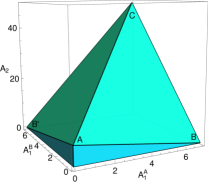
Figure 5: The polytope of bipartite separable states of $d\otimes d$-dimensional systems in terms of the quantities $A_{1}^{A},A_{1}^{B},$ and $A_{2}$, where $d=8$. The two triangular surfaces on the top originate from the constraints in Eq. (S.38) and are covered by states $\varrho(p,\theta)$ from the family in Eq. (S.39). The vertices of the triangle correspond to parameters $p=1/d$, $\theta={\pi}/2$ (A), $p=1/d$, $\theta=0$ (B’) and $p=1$ (C). Point (B) is obtained by exchanging the role of A and B in $\varrho(1/d,0)$. Note that the construction of the surface also requires the knowledge of the entire polytope, this is derived in Section A7.

A7. Characterization of two-qudit states and discussion of the separability criterion

First, let us characterize two-qudit states using sector lengths. This characterization can be useful for understanding the two-qudit separability criterion geometrically. The previous work [36] has illustrated the set of admissible $(A_{1},A_{2})$ pairs in two-qubit systems, we will generalize it to two-qudit systems. We begin by recalling that any two-qudit state can be written as

$$\varrho_{AB}=\frac{1}{d^{2}}\sum_{i,j=0}^{d^{2}-1}t_{ij}\lambda_{i}\otimes\lambda_{j}=\frac{1}{d^{2}}\left(\mathbbm{1}^{\otimes 2}+P_{1}+P_{2}\right),$$ (16)

where the Hermitian operators $P_{k}$ for $k=1,2$ denote the sum of all terms in the basis element weight $k$. The relation (S.5) allows us to translate the purity bound $\mathrm{tr}(\varrho_{AB}^{2})\leq 1$ to

$$1+A_{1}+A_{2}\leq d^{2}.$$ (S.46)

Remember that $A_{1}=A_{1}^{A}+A_{1}^{B}$. As examples of pure states, consider product states $\ket{{\mathrm{prod}}_{j}}=\ket{jj}$ with the computational basis for $j=0,1,\ldots,(d-1)$. The pure product states have $A_{1}^{A}=A_{1}^{B}=d-1$, $A_{1}=2(d-1)$, and $A_{2}=(d-1)^{2}$. Also, the maximally entangled state $\ket{\Phi^{+}_{d}}=(1/{\sqrt{d}})\sum_{i=0}^{d-1}\ket{ii}$ has $A_{1}^{A}=A_{1}^{B}=A_{1}=0$ and $A_{2}=d^{2}-1$. It is important to note that the pure product states and the maximally entangled state can, respectively, maximize the admissible values of $A_{1}$ and $A_{2}$ for all two-qudit states (see Ref. [37]). That is, both values of sector lengths give tight upper bounds for all two-qudit states: $A_{1}\leq 2(d-1)$ and $A_{2}\leq d^{2}-1$. Due to the purity condition (S.46), any pure two-qudit state must satisfy $A_{1}\in[0,2(d-1)]$ and $A_{2}=d^{2}-1-A_{1}$.

To see another constraint on sector lengths, let us introduce the state inversion [52, 53] expressed as

$$\tilde{\varrho}_{AB}=\frac{1}{d^{2}}\left\{(d-1)^{2}\mathbbm{1}^{\otimes 2}-(d-1)P_{1}+P_{2}\right\}.$$ (S.47)

Since $\tilde{\varrho}_{AB}$ is positive, we have

$$0\leq\mathrm{tr}(\varrho_{AB}\tilde{\varrho}_{AB}).$$ (S.48)

From the relation (S.5) and the expression (16), the condition (S.48) leads to the state inversion bound:

$$0\leq(d-1)^{2}-(d-1)A_{1}+A_{2}.$$ (S.49)

Here, if $A_{2}=0$, then $A_{1}\leq d-1$, where equality holds if a state is given by, for example, $\ket{0}\!\bra{0}\otimes{\mathbbm{1}}/{d}$.

In conclusion, we obtained the tight four bounds: $A_{1}\leq 2(d-1)$, $A_{2}\leq d^{2}-1$, and Eqs. (S.46, S.49). These linear constraints on $A_{1}$ and $A_{2}$ allow us to ensure the positivity of two-qudit states and to find the total set of their admissible values. The geometrical expressions are displayed in Figs. 6 and 7.

Next, let us consider entanglement detection of two-qudit states. One existing criterion states that any two-qudit separable state obeys $A_{2}\leq(d-1)^{2}$ [23], where an example of states obeying $A_{2}=(d-1)^{2}$ is $\ket{{\mathrm{prod}}_{j}}$. In particular, the maximally entangled state $\ket{\Phi^{+}_{d}}$ maximally violates this inequality. Now, we look at the gap between the maximally entangled state and the pure product state

$$\frac{A_{2}(\Phi^{+}_{d})}{A_{2}({\mathrm{prod}}_{j})}=\frac{d^{2}-1}{(d-1)^{2}}\to 1$$ (S.50)

for large $d$. This scaling tells us that the simple criterion cannot be useful in very high-dimensional systems. On the other hand, the criteria (S.35, S.44) allow us to detect entanglement much more powerfully than the existing criterion, since they are expressed as the tilted bounds geometrically in Figs. 6 and 7. To see that, we consider the two-qudit isotropic state:

$$\varrho_{\mathrm{iso}}=p\ket{\Phi^{+}_{d}}\!\bra{\Phi^{+}_{d}}+\frac{1-p}{d^{2}}\mathbbm{1}^{\otimes 2},$$ (S.51)

which has $(A_{1},A_{2})=(0,p^{2}(d^{2}-1))$. The existing criterion $A_{2}\leq(d-1)^{2}$ detects this state as entangled for $p>\sqrt{d-1}/\sqrt{d+1}$, while Eq. (S.44) detects it already for $p>1/\sqrt{d+1}$, and the state is known to be entangled iff $p>1/(d+1)$.

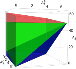
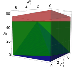
Figure 6: Geometry of the state space of $d\otimes d$-dimensional systems in terms of the quantities $A_{1}^{A},A_{1}^{B},$ and $A_{2}$, where $d=8$. The total polytope is the set of all states, characterized by the inequalities $0\leq A_{1}^{A},A_{1}^{B}\leq d-1$, $0\leq A_{2}\leq d^{2}-1$, $A_{1}^{A}+A_{1}^{B}+A_{2}\leq d^{2}-1$, and $0\leq(d-1)^{2}-(d-1)(A_{1}^{A}+A_{1}^{B})+A_{2}$. The separable states are contained in the blue polytope, obeying the additional constraint in Eq. (S.35). The red area corresponds to the states violating a previously known criterion for separable states, $A_{2}\leq(d-1)^{2}$ [23]. Thus, the green area marks the improvement coming from Observation 3 compared with the previous result.

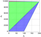
Figure 7: Geometry of the state space of $d\otimes d$-dimensional systems in terms of the second moments $A_{1}$ and $A_{2}$, where $d=100$. The total figure is the set of all states, characterized by the same inequalities with Fig. 6 in the case $A_{1}^{A}=A_{1}^{B}$. The separable states are contained in the blue area, obeying the additional bound (S.44). The red are corresponds to the state violating a previously known criterion for separable states, $A_{2}\leq(d-1)^{2}$ [23]. Thus, the green area marks the improvement of the criterion in Observation 3 compared with the previous result.

Appendix B: Moments of random correlations in higher-dimensional systems

In Appendix B, we first evaluate the expressions of $\mathcal{S}_{AB}^{(r)}$ for $r=2$ and $r=4$, originating from the orthogonal average, in terms of the correlation matrix. The calculations are stated rather explicitly here to highlight the methods used. Second, we show that a certain choice of observables yields the same results when performing random unitary measurements instead, i.e., evaluating $\mathcal{R}_{AB}^{(2)}$ and $\mathcal{R}_{AB}^{(4)}$, where we skip the detailed calculations, as they follow similar lines as the detailed orthogonal ones.

B1. Evaluation of $\mathcal{S}_{AB}^{(2)}$ and $\mathcal{S}_{AB}^{(4)}$ for a given state

In the following, we will show that the moments defined in Eq. (11) in the main text are given by

$$\mathcal{S}^{(2)}_{AB} =V\sum_{i,j}t_{ij}^{2},$$ (S.52)

$$\mathcal{S}^{(4)}_{AB} =W\left\{3\sum_{i,j}t_{ij}^{4}+3\sum_{i,j,k,i\neq j}t_{ik}^{2}t_{jk}^{2}+3\sum_{i,j,k,i\neq j}t_{ki}^{2}t_{kj}^{2}+\sum_{i,j,k,l,i\neq k,j\neq l}\left(t_{ij}^{2}t_{kl}^{2}+2t_{ij}t_{il}t_{kj}t_{kl}\right)\right\},$$ (S.53)

where the $t_{ij}$ are the coefficients from Eq. (8) in the main text and

$$V=\frac{1}{(d-1)^{2}},\ \ \ \ W=\frac{1}{3\left(d-1\right)^{4}}.$$ (S.54)

Let us substitute the two-qudit state (8) in the main text into the moments $\mathcal{S}^{(r)}_{AB}$. In the following, we always add a normalization $N=N(r,d)$, which is later chosen such that $\mathcal{S}^{(r)}_{AB}=1$ for pure product states, see also Eq. (S.84) below. Then we have

$$\mathcal{S}^{(r)}_{AB} =N\int d\bm{\alpha}_{1}\int d\bm{\alpha}_{2}\,\left\{\mathrm{tr}\left[\left(\frac{1}{d^{2}}\sum_{i,j=0}^{d^{2}-1}t_{ij}\lambda_{i}\otimes\lambda_{j}\right)\bm{\alpha}_{1}\cdot\bm{\lambda}\otimes\bm{\alpha}_{2}\cdot\bm{\lambda}\right]\right\}^{r}$$

$$=\frac{N}{d^{2r}}\int d\bm{\alpha}_{1}\int d\bm{\alpha}_{2}\,\left\{\sum_{i,j=1}^{d^{2}-1}t_{ij}\mathrm{tr}\left[\lambda_{i}\bm{\alpha}_{1}\cdot\bm{\lambda}\right]\cdot\mathrm{tr}\left[\lambda_{j}\bm{\alpha}_{2}\cdot\bm{\lambda}\right]\right\}^{r}$$

$$=N\int d\bm{\alpha}_{1}\int d\bm{\alpha}_{2}\,\left[\sum_{i,j=1}^{d^{2}-1}t_{ij}{\alpha}_{1}^{(i)}{\alpha}_{2}^{(j)}\right]^{r}$$

$$=N\int d\bm{\alpha}_{1}\int d\bm{\alpha}_{2}\,\sum_{r_{i,j}}\frac{r!}{r_{1,1}!\cdots r_{d^{2}-1,\,d^{2}-1}!}\prod_{i,j=1}^{d^{2}-1}\left[t_{ij}{\alpha}_{1}^{(i)}{\alpha}_{2}^{(j)}\right]^{r_{i,j}}$$

$$=N\sum_{r_{i,j}}\frac{r!}{r_{1,1}!\cdots r_{d^{2}-1,\,d^{2}-1}!}\prod_{i,j=1}^{d^{2}-1}t_{ij}^{r_{i,j}}\int d\bm{\alpha}_{1}\,\prod_{i=1}^{d^{2}-1}\left[{\alpha}_{1}^{(i)}\right]^{\sum_{j=1}^{d^{2}-1}r_{i,j}}\int d\bm{\alpha}_{2}\,\prod_{j=1}^{d^{2}-1}\left[{\alpha}_{2}^{(j)}\right]^{\sum_{i=1}^{d^{2}-1}r_{i,j}}$$

$$=N\sum_{r_{i,j}}\frac{r!}{r_{1,1}!\cdots r_{d^{2}-1,\,d^{2}-1}!}\prod_{i,j=1}^{d^{2}-1}t_{ij}^{r_{i,j}}\int d\bm{\alpha}_{1}\,\prod_{i=1}^{d^{2}-1}\left[{\alpha}_{1}^{(i)}\right]^{a_{i}}\int d\bm{\alpha}_{2}\,\prod_{j=1}^{d^{2}-1}\left[{\alpha}_{2}^{(j)}\right]^{a^{\prime}_{j}}$$

$$=4N\sum_{r_{i,j}}\frac{r!}{r_{1,1}!\cdots r_{d^{2}-1,\,d^{2}-1}!}\prod_{i,j=1}^{d^{2}-1}t_{ij}^{r_{i,j}}B(b_{1},b_{2},\ldots,b_{d^{2}-1})B(b^{\prime}_{1},b^{\prime}_{2},\ldots,b^{\prime}_{d^{2}-1}),$$ (S.55)

where we use $\mathrm{tr}(\bm{\alpha}_{i}\cdot\bm{\lambda})=0$ and the multinomial theorem

$$\left(\sum_{i=1}^{n}x_{i}\right)^{r}=\sum_{r_{1}+r_{2}+\cdots+r_{n}=r}\frac{r!}{r_{1}!r_{2}!\cdots r_{n}!}\prod_{i=1}^{n}x_{i}^{r_{i}}.$$ (S.56)

The sum $\sum_{r_{i,j}}$ means $\sum_{r_{1,1}+\cdots+r_{1,\,d^{2}-1}+r_{2,1}+\cdots+r_{d^{2}-1,\,d^{2}-1}=r}$. We define that $a_{i}=\sum_{j=1}^{d^{2}-1}r_{i,j}$, $a^{\prime}_{j}=\sum_{i=1}^{d^{2}-1}r_{i,j}$, $b_{i}=(a_{i}+1)/2$, and $b^{\prime}_{j}=(a^{\prime}_{j}+1)/2$. Note that in general, the integral over the $n$-dimensional unit sphere is written as $2B(\beta_{1},\beta_{2},\ldots,\beta_{n})$ (see Ref. [54]), where $B(\beta_{1},\beta_{2},\ldots,\beta_{n})$ denotes the multi-variable beta function, for $\beta_{i}=(\alpha_{i}+1)/2$ and the gamma function $\Gamma(\beta_{i})$, given by

$$B(\beta_{1},\beta_{2},\ldots,\beta_{n})=\frac{\Gamma(\beta_{1})\Gamma(\beta_{2})\cdots\Gamma(\beta_{n})}{\Gamma(\beta_{1}+\beta_{2}+\ldots+\beta_{n})}.$$ (S.57)

This integral vanishes if any of $\alpha_{i}$ is odd.

Case of $r=2$

Let us evaluate the moment at $r=2$. The condition $r=2$ means $r_{1,1}+\cdots+r_{d^{2}-1,\,d^{2}-1}=2$. To make this more explicit, we introduce the square matrix $\bm{R}$

$$\bm{R}=\begin{pmatrix}r_{1,1}&r_{1,2}&\cdots&r_{1,\,d^{2}-1}\\ r_{2,1}&r_{2,2}&\cdots&r_{2,\,d^{2}-1}\\ \vdots&\vdots&\ddots&\vdots\\ r_{d^{2}-1,1}&r_{d^{2}-1,2}&\cdots&r_{d^{2}-1,\,d^{2}-1}\end{pmatrix}.$$ (S.58)

Recall here that $a_{i}=\sum_{j=1}^{d^{2}-1}r_{i,j}$ and $a^{\prime}_{j}=\sum_{i=1}^{d^{2}-1}r_{i,j}$. Thus, $a_{i}$ and $a^{\prime}_{j}$ respectively correspond to the $i$-th row vector and the $j$-th column vector of the matrix $\bm{R}$.

There are two candidates that satisfy the condition $r_{1,1}+\cdots+r_{d^{2}-1,\,d^{2}-1}=2$:

• one of elements is equal to $2$ and all other elements are zero, that is, fixed $r_{\alpha,\beta}=2$ and $r_{k,l\neq\alpha,\beta}=0$. An example is given by

  $$\bm{R}=\begin{pmatrix}2&0&\cdots&0\\ 0&0&\cdots&0\\ \vdots&\vdots&\ddots&\vdots\\ 0&0&\cdots&0\end{pmatrix}.$$ (S.59)

• two of elements are equal to $1$ and all other elements are zero, that is, fixed $r_{\alpha,\beta}=r_{\gamma,\delta}=1$ and all other $r_{k,l}=0$. Examples are

  $$\bm{R}=\begin{pmatrix}0&1&\cdots&0\\ 0&1&\cdots&0\\ \vdots&\vdots&\ddots&\vdots\\ 0&0&\cdots&0\end{pmatrix},\ \ \begin{pmatrix}1&1&\cdots&0\\ 0&0&\cdots&0\\ \vdots&\vdots&\ddots&\vdots\\ 0&0&\cdots&0\end{pmatrix},\ \ \begin{pmatrix}1&0&\cdots&0\\ 0&1&\cdots&0\\ \vdots&\vdots&\ddots&\vdots\\ 0&0&\cdots&0\end{pmatrix}.$$ (S.60)

In any case of the candidate (2), either or both of $a_{i}$ and $a^{\prime}_{j}$ are always $1$, that is, odd. This results in the vanishing of the integral over the sphere. Accordingly, it is sufficient to focus only on the candidate (1) in Eq. (S.59). Concerning the expression of moments (S.55), we have

$$\frac{2!}{0!\cdots 2!\cdots 0!}=1,\ \ \prod_{i,j=1}^{d^{2}-1}t_{ij}^{r_{i,j}}=t_{\alpha\beta}^{2},$$

$$a_{\alpha}=\sum_{j}r_{\alpha,j}=2,\ a_{i\neq\alpha}=0,\ \ a^{\prime}_{\beta}=\sum_{i}r_{i,\beta}=2,\ a^{\prime}_{i\neq\beta}=0,$$

$$b_{\alpha}=\frac{3}{2},\ b_{i\neq\alpha}=\frac{1}{2},\ \ b^{\prime}_{\beta}=\frac{3}{2},\ b^{\prime}_{i\neq\beta}=\frac{1}{2},$$

$$B(b_{1},\ldots,b_{\alpha},\ldots,b_{d^{2}-1})=B(b^{\prime}_{1},\ldots,b^{\prime}_{\beta},\ldots,b^{\prime}_{d^{2}-1})=B\left(\frac{1}{2},\ldots,\frac{3}{2},\ldots,\frac{1}{2}\right)=\frac{(\sqrt{\pi})^{d^{2}-1}}{2\Gamma\left(\frac{d^{2}+1}{2}\right)}.$$ (S.61)

Then we have

$$\mathcal{S}^{(2)}_{AB}=V\sum_{i,j}t_{ij}^{2},$$ (S.62)

where

$$V=4N\frac{\pi^{d^{2}-1}}{4\left[\Gamma\left(\frac{d^{2}+1}{2}\right)\right]^{2}}=\frac{1}{(d-1)^{2}}.$$ (S.63)

Case of $r=4$

Let us evaluate the moment at $r=4$. The condition $r=4$ means $r_{1,1}+\cdots+r_{d^{2}-1,\,d^{2}-1}=4$. There are several candidates that satisfy the condition $r_{1,1}+\cdots+r_{d^{2}-1,\,d^{2}-1}=4$. In the following, we will only describe the three candidates with nonzero values of the integral over the sphere.

• one of the elements is equal to $4$ and all other elements are zero, that is, fixed $r_{\alpha,\beta}=4$ and $r_{k,l\neq\alpha,\beta}=0$. An example is

  $$\bm{R}=\begin{pmatrix}4&0&\cdots&0\\ 0&0&\cdots&0\\ \vdots&\vdots&\ddots&\vdots\\ 0&0&\cdots&0\end{pmatrix}.$$ (S.64)

• two of elements are equal to $2$ and all other elements are zero, that is, fixed $r_{\alpha,\beta}=r_{\gamma,\delta}=2$ and others $r_{k,l}=0$. Examples are divided into three types.

  $$\bm{R}=\begin{pmatrix}0&2&\cdots&0\\ 0&2&\cdots&0\\ \vdots&\vdots&\ddots&\vdots\\ 0&0&\cdots&0\end{pmatrix},\ \ \begin{pmatrix}2&2&\cdots&0\\ 0&0&\cdots&0\\ \vdots&\vdots&\ddots&\vdots\\ 0&0&\cdots&0\end{pmatrix},\ \ \begin{pmatrix}2&0&\cdots&0\\ 0&2&\cdots&0\\ \vdots&\vdots&\ddots&\vdots\\ 0&0&\cdots&0\end{pmatrix}.$$ (S.65)

  We call these (a), (b), and (c) cases, respectively.

• four of elements are equal to $1$ and all other elements are zero, that is, fixed $r_{\alpha,\beta}=r_{\gamma,\delta}=r_{\epsilon,\zeta}=r_{\eta,\theta}=1$ and others are zero. An example is

  $$\bm{R}=\begin{pmatrix}1&1&\cdots&0\\ 1&1&\cdots&0\\ \vdots&\vdots&\ddots&\vdots\\ 0&0&\cdots&0\end{pmatrix}.$$ (S.66)

Candidate (1). Let us consider the candidate (1). For fixed $r_{\alpha,\beta}=4$ and $r_{k,l\neq\alpha,\beta}=0$, we have

$$a_{\alpha}=4,\ a^{\prime}_{\beta}=4,\ \ b_{\alpha}=\frac{5}{2},\ b^{\prime}_{\beta}=\frac{5}{2},$$

$$B(b_{1},\ldots,b_{\alpha},\ldots,b_{d^{2}-1})=B(b^{\prime}_{1},\ldots,b^{\prime}_{\beta},\ldots,b^{\prime}_{d^{2}-1})=B\left(\frac{1}{2},\ldots,\frac{5}{2},\ldots,\frac{1}{2}\right)=\frac{3(\sqrt{\pi})^{d^{2}-1}}{4\Gamma\left(\frac{d^{2}+3}{2}\right)}.$$ (S.67)

Therefore, the corresponding term is given by

$$4N\frac{9\pi^{d^{2}-1}}{16\left[\Gamma\left(\frac{d^{2}+3}{2}\right)\right]^{2}}\sum_{i,j}t_{ij}^{4}.$$ (S.68)

Candidate (2). Let us consider the candidate (2). For fixed $r_{\alpha,\beta}=r_{\gamma,\delta}=2$, we have the three types (a), (b), and (c), as the three examples described in (S.65):

• $\alpha\neq\gamma$ and $\beta=\delta$.

• $\alpha=\gamma$ and $\beta\neq\delta$.

• $\alpha\neq\gamma$ and $\beta\neq\delta$.

For the type (a), we have

$$a_{n}=2,\ \mathrm{for}\,n=\alpha,\gamma,\ a^{\prime}_{\beta}=4,\ \ b_{n}=\frac{3}{2},\ b^{\prime}_{\beta}=\frac{5}{2},$$

$$B(b_{1},\ldots,b_{\alpha},\ldots,b_{\gamma},\ldots,b_{d^{2}-1})=B\left(\frac{1}{2},\ldots,\frac{3}{2},\ldots,\frac{3}{2},\ldots,\frac{1}{2}\right)=\frac{(\sqrt{\pi})^{d^{2}-1}}{4\Gamma\left(\frac{d^{2}+3}{2}\right)},$$

$$B(b^{\prime}_{1},\ldots,b^{\prime}_{\beta},\ldots,b^{\prime}_{d^{2}-1})=B\left(\frac{1}{2},\ldots,\frac{5}{2},\ldots,\frac{1}{2}\right)=\frac{3(\sqrt{\pi})^{d^{2}-1}}{4\Gamma\left(\frac{d^{2}+3}{2}\right)}.$$ (S.69)

Moreover, to avoid the over-counting of summation, we multiply it by $1/2$ in order to be able to write the contribution as the following sum:

$$4N\times 6\times\frac{1}{2}\times\frac{3\pi^{d^{2}-1}}{16\left[\Gamma\left(\frac{d^{2}+3}{2}\right)\right]^{2}}\sum_{i,j,k,i\neq j}t_{ik}^{2}t_{jk}^{2}.$$ (S.70)

For the type (b), we have the similar result with (a):

$$4N\times 6\times\frac{1}{2}\times\frac{3\pi^{d^{2}-1}}{16\left[\Gamma\left(\frac{d^{2}+3}{2}\right)\right]^{2}}\sum_{i,j,k,i\neq j}t_{ki}^{2}t_{kj}^{2}.$$ (S.71)

For the type (c), we have

$$a_{n}=2,\ a^{\prime}_{m}=2,\ \mathrm{for}\,n=\alpha,\gamma,\ m=\beta,\delta,\ \ b_{n}=\frac{3}{2},\ b^{\prime}_{m}=\frac{3}{2},$$

$$B(b_{1},\ldots,b_{\alpha},\ldots,b_{\gamma},\ldots,b_{d^{2}-1})=B(b^{\prime}_{1},\ldots,b^{\prime}_{\beta},\ldots,b^{\prime}_{\delta},\ldots,b^{\prime}_{d^{2}-1})=B\left(\frac{1}{2},\ldots,\frac{3}{2},\ldots,\frac{3}{2},\ldots,\frac{1}{2}\right)=\frac{(\sqrt{\pi})^{d^{2}-1}}{4\Gamma\left(\frac{d^{2}+3}{2}\right)}.$$ (S.72)

Therefore, the corresponding term is given by

$$4N\times 6\times\frac{1}{2}\times\frac{\pi^{d^{2}-1}}{16\left[\Gamma\left(\frac{d^{2}+3}{2}\right)\right]^{2}}\sum_{i,j,k,l,i\neq k,j\neq l}t_{ij}^{2}t_{kl}^{2}.$$ (S.73)

Candidate (3). Let us consider the candidate (3). For fixed $r_{\alpha,\beta}=r_{\gamma,\delta}=r_{\epsilon,\zeta}=r_{\eta,\theta}=1$, only one case yields finite values of the integral: $\alpha=\gamma$, $\beta=\zeta$, $\epsilon=\eta$, and $\delta=\theta$. Here, rewriting the condition as $r_{\alpha,\beta}=r_{\alpha,\delta}=r_{\epsilon,\beta}=r_{\epsilon,\delta}=1$, we have

$$a_{n}=2,\ a^{\prime}_{m}=2,\ \mathrm{for}\,n=\alpha,\epsilon,\ m=\beta,\delta,\ \ b_{n}=\frac{3}{2},\ b^{\prime}_{m}=\frac{3}{2},$$

$$B(b_{1},\ldots,b_{\alpha},\ldots,b_{\epsilon},\ldots,b_{d^{2}-1})=B(b^{\prime}_{1},\ldots,b^{\prime}_{\beta},\ldots,b^{\prime}_{\delta},\ldots,b^{\prime}_{d^{2}-1})=B\left(\frac{1}{2},\ldots,\frac{3}{2},\ldots,\frac{3}{2},\ldots,\frac{1}{2}\right)=\frac{(\sqrt{\pi})^{d^{2}-1}}{4\Gamma\left(\frac{d^{2}+3}{2}\right)}.$$ (S.74)

Moreover, to avoid the over-counting of summation, we multiply it by $1/4$. Therefore, the corresponding term is given by

$$4N\times 24\times\frac{1}{4}\times\frac{\pi^{d^{2}-1}}{16\left[\Gamma\left(\frac{d^{2}+3}{2}\right)\right]^{2}}\sum_{i,j,k,l,i\neq k,j\neq l}t_{ij}t_{il}t_{kj}t_{kl}.$$ (S.75)

According to the candidates (1), (2), and (3), we finally arrive at

$$\mathcal{S}^{(4)}_{AB}=W\left\{3\sum_{i,j}t_{ij}^{4}+3\sum_{i,j,k,i\neq j}t_{ik}^{2}t_{jk}^{2}+3\sum_{i,j,k,i\neq j}t_{ki}^{2}t_{kj}^{2}+\sum_{i,j,k,l,i\neq k,j\neq l}\left(t_{ij}^{2}t_{kl}^{2}+2t_{ij}t_{il}t_{kj}t_{kl}\right)\right\},$$ (S.76)

where

$$W=4N\frac{3\pi^{d^{2}-1}}{16\left[\Gamma\left(\frac{d^{2}+3}{2}\right)\right]^{2}}=\frac{1}{3\left(d-1\right)^{4}}.$$ (S.77)

B2. Suitable observables in higher dimensions

Let us discuss the relation between the moments $\mathcal{R}^{(r)}_{AB}$ and $\mathcal{S}^{(r)}_{AB}$. In order to explain the difficulties for higher dimensions, let us focus on qubits first. Suppose that Alice and Bob locally perform the measurements $M_{A}$ and $M_{B}$ in random bases parametrized by the unitary transformations $U_{A},U_{B}\in\mathcal{U}(d)$, such that

$$\left\{\ket{u_{0}}_{A}=U_{A}\ket{0}_{A},\ket{u_{1}}_{A}=U_{A}\ket{1}_{A},\ldots,\ket{u_{d-1}}_{A}=U_{A}\ket{d-1}_{A}\right\},$$ (S.78)

$$\left\{\ket{u_{0}}_{B}=U_{B}\ket{0}_{B},\ket{u_{1}}_{B}=U_{B}\ket{1}_{B},\ldots,\ket{u_{d-1}}_{B}=U_{B}\ket{d-1}_{B}\right\}.$$ (S.79)

In the case of qubits ($d=2$), Alice’s (Bob’s) measurement direction corresponds to a random three-dimensional unit vector $\bm{u}_{A}$ ($\bm{u}_{B}$) chosen uniformly on the Bloch sphere $\mathcal{S}^{2}$. Then, the expectation value is given by $\mathrm{tr}\left[\varrho_{AB}\sigma_{\bm{u}_{A}}\otimes\sigma_{\bm{u}_{B}}\right]$, where $\sigma_{\bm{u}}=\bm{u}\cdot\bm{\sigma}$ is the rotated Pauli matrix with the vector of the usual Pauli matrices ${\bm{\sigma}}=(\sigma_{x},\sigma_{y},\sigma_{z})^{\top}$. Without loss of generality, one can take the Pauli-$Z$ matrix $\sigma_{z}$ as the observables $M_{A}$ and $M_{B}$. Then we can characterize the obtained distribution via its moments $\mathcal{R}^{(r)}_{AB}$

$$\mathcal{R}^{(r)}_{AB}=\int dU_{A}\int dU_{B}\left\{\mathrm{tr}[\varrho_{AB}(U_{A}\sigma_{z}U_{A}^{\dagger})\otimes(U_{B}\sigma_{z}U_{B}^{\dagger})]\right\}^{r}=\frac{1}{(4\pi)^{2}}\int_{\mathcal{S}^{2}}d\bm{u}_{A}\int_{\mathcal{S}^{2}}d\bm{u}_{B}\left[\mathrm{tr}\left(\varrho_{AB}\sigma_{\bm{u}_{A}}\otimes\sigma_{\bm{u}_{B}}\right)\right]^{r},$$ (S.80)

where the unitaries are typically chosen according to the Haar distribution. For all odd $r$, the moments $\mathcal{R}^{(r)}_{AB}$ vanish, so the quantities of interest are the moments of even $r$. Indeed, the second moment $\mathcal{R}^{(2)}_{AB}$ can be evaluated by a unitary two-design [32]:

$$\mathcal{R}^{(2)}_{AB}=\frac{1}{9}\sum_{\bm{e}_{A},\bm{e}_{B}=\bm{e}_{1},\bm{e}_{2},\bm{e}_{3}}\mathrm{tr}\left[\varrho_{AB}\sigma_{\bm{e}_{A}}\otimes\sigma_{\bm{e}_{B}}\right]^{2}=\frac{1}{9}\sum_{i,j=1}^{3}t_{ij}^{2},$$ (S.81)

where $\{\pm\bm{e}_{k}\mid k=1,2,3\}$ are the orthogonal local directions and the $t_{ij}$ are two-body correlation coeffients with $1\leq i,j\leq 3$ of $\varrho_{AB}$, where we call this submatix $T_{s}$. It is important that the moments $\mathcal{R}^{(r)}_{AB}$ are by definition invariant under local unitary transformations $U_{A}\otimes U_{B}$. This property allows us to find a local unitary such that the matrix $T_{s}$ can be diagonalized by a orthogonal transformation, due to the isomorphism between $SO(3)$ and $SU(2)$.

On the other hand, in the case of higher dimensions ($d>2$), there are several problems. First, the notion of a Bloch sphere is not available. Due to this fact, not all possible observables are equivalent under randomized unitaries. Second, for a odd $r$, the moments $\mathcal{R}^{(r)}_{AB}$ in Eq. (2) in the main text do not vanish, see Ref. [55]. Third, for $r=2$, the second moments are independent of the choice of observables as long as the observables are traceless (see Theorem 9 in Ref. [23]), while higher moments depend on the choice. To approach these problems, we make use of the quantities from the previous section, i.e.,

$$\mathcal{S}^{(r)}_{AB} =N(r,d)\int_{\mathcal{V}^{d^{2}-2}}d\bm{\alpha}_{1}\int_{\mathcal{V}^{d^{2}-2}}d\bm{\alpha}_{2}[\mathrm{tr}(\varrho_{AB}\bm{\alpha}_{1}\cdot\bm{\lambda}\otimes\bm{\alpha}_{2}\cdot\bm{\lambda})]^{r}$$ (S.82)

$$\propto\int dO_{A}\int dO_{B}\left\{\mathrm{tr}\left[\sum_{i,j}\left((O_{A}T_{s}O_{B})_{ij}(\lambda_{i}\otimes\lambda_{j})\right)(\lambda_{1}\otimes\lambda_{1})\right]\right\}^{r},$$ (S.83)

where $O_{A},O_{B}\in SO(d^{2}-1)$ are non-physical orthogonal matrices and the elements of the correlation matrix $T_{s}$ are given by $(T_{s})_{ij}=\mathrm{tr}(\varrho_{AB}\lambda_{i}\otimes\lambda_{j})$. In addition, the $\bm{\alpha}_{i}$ denote the $(d^{2}-1)$-dimensional unit real vectors uniformly chosen from on the pseudo Bloch sphere $\mathcal{V}^{d^{2}-2}$, and $\bm{\lambda}=(\lambda_{1},\lambda_{2},\ldots,\lambda_{d^{2}-1})$ is the vector of Gell-Mann matrices. Here, $N(r,d)$ is a normalization factor such that ${\mathcal{S}}^{(r)}_{AB}=1$ at pure product states:

$$N(r,d)=\frac{[(d^{2}+r-3)!!]^{2}}{(d-1)^{r}[(r-1)!!]^{2}[(d^{2}-3)!!]^{2}}\left(\frac{\Gamma(\frac{d^{2}-1}{2})}{2\sqrt{\pi}^{d^{2}-1}}\right)^{2},$$ (S.84)

where, for a positive number $n$, $n!!$ is the double factorial and $\Gamma(n)$ is the gamma function. The moments $\mathcal{S}^{(r)}_{AB}$ are analytically calculable, so we take $\mathcal{S}^{(r)}_{AB}$ as the starting point for our discussion.

The question here is whether it is possible to find observables such that $\mathcal{R}^{(r)}_{AB}$ coincides with $\mathcal{S}^{(r)}_{AB}$, up to a constant. While the observables $M_{A}$ and $M_{B}$ do not have to be diagonal, they can be assumed to be diagonal in the unitary group averaging. Now let us consider a diagonal observable such that $M_{A}=M_{B}=M_{d}$. Then, we are in a position to present the suitable choice of $M_{d}$ for the coincidence between $\mathcal{S}^{(r)}_{AB}$ and $\mathcal{R}^{(r)}_{AB}$.

Observation 9. In $d$-dimensional quantum systems where $d$ is odd, let the diagonal observable $M_{d}$ be given by

$$M_{d}=\operatorname{diag}(\underbrace{\alpha_{+},\ldots,\alpha_{+}}_{(d-1)/2},\beta_{y},\underbrace{\alpha_{-},\ldots,\alpha_{-}}_{(d-1)/2}),$$ (S.85)

where

$$\alpha_{\pm} =\frac{\pm d-2y+1}{\sqrt{(d-1)[(2y-1)^{2}+d)]}},$$ (S.86)

$$\beta_{y} =-\sqrt{\frac{(d-1)(2y-1)^{2}}{(2y-1)^{2}+d}},$$ (S.87)

$$y =\frac{1}{2}\left[1-\sqrt{1+\frac{d+3+\sqrt{d^{3}+3d^{2}+d+3}}{d-2}}\right],$$ (S.88)

and $\mathrm{tr}(M_{d})=0$ and $\mathrm{tr}(M_{d}^{2})=d$. Then, measuring the observable $M_{d}$ yields

$$\mathcal{S}^{(2)}_{AB}=(d+1)^{2}\mathcal{R}^{(2)}_{AB},\ \ \ \ \ \ \ \ \mathcal{S}^{(4)}_{AB}=\frac{(d+1)^{2}(d^{2}+1)^{2}}{9(d-1)^{2}}\mathcal{R}^{(4)}_{AB}.$$ (S.89)

Proof.

Analogous to the calculation in the case of $\mathcal{S}^{(r)}_{AB}$ shown in Eq. (S.55), after some lengthy calculation and using the fact that $M_{d}$ is traceless, we obtain

$$\mathcal{R}^{(r)}_{AB}=\sum_{r_{i,j}}\frac{r!}{r_{1,1}!\cdots r_{d^{2}-1,\,d^{2}-1}!}\prod_{i,j=1}^{d^{2}-1}t_{ij}^{r_{i,j}}\int dU_{A}\prod_{i=1}^{d^{2}-1}\mathrm{tr}[U_{A}M_{d}U_{A}^{\dagger}\lambda_{i}]^{a_{i}}\int dU_{B}\prod_{j=1}^{d^{2}-1}\mathrm{tr}[U_{B}M_{d}U_{B}^{\dagger}\lambda_{j}]^{a^{\prime}_{j}},$$ (S.90)

where the sum spans over all non-negative integer assignments to the $r_{i,j}$ such that $\sum_{i,j=1}^{d^{2}-1}r_{i,j}=r$, and $a_{i}=\sum_{j=1}^{d^{2}-1}r_{i,j}$, $a_{j}^{\prime}=\sum_{i=1}^{d^{2}-1}r_{i,j}$.

We start with the discussion of the case $r=4$, where we focus on one of the integrals and evaluate it for all possible exponent vectors $\vec{a}=(a_{1},\ldots,a_{d^{2}-1})$. As all the entries are positive integers that sum to $4$, there are five families of vectors to be considered:

• $a_{k}=4$, $a_{l\neq k}=0$,

• $a_{k}=3$, $a_{l}=1$, $a_{m\neq k,l}=0$,

• $a_{k}=2$, $a_{l}=2$, $a_{m\neq k,l}=0$,

• $a_{k}=2$, $a_{l}=1$, $a_{m}=1$, $a_{n\neq k,l,m}=0$,

• $a_{k}=1$, $a_{l}=1$, $a_{m}=1$, $a_{n}=1$, $a_{o\neq k,l,m,n}=0$.

We aim to prove that the whole integral coincides with the one obtained from integration over the orthogonal group. To that end, we compare the integrals occurring in Eq. (S.90) with those in Eq. (S.55). In particular, we try to tweak the observable such that for all vectors $\vec{a}$ with $\sum a_{i}=4$,

$$\int dU_{A}\prod_{i=1}^{d^{2}-1}\mathrm{tr}[U_{A}M_{d}U_{A}^{\dagger}\lambda_{i}]^{a_{i}}=MB(b_{1},b_{2},\ldots,b_{d^{2}-1}),$$ (S.91)

where $B$ is defined in Eq. (S.57) and $b_{i}=(a_{i}+1)/2$. The prefactor $M$ can be absorbed into the observable, as long as it is independent from $\vec{a}$. To certify equality, we will show

1. that the cases (b), (d) and (e) vanish for all choices of $k,l,m,n$, as they contain odd numbers,

2. that the results of all integrals in the family (a) coincide, as well as those in family (c), as the function $B$ is symmetric w.r.t. its parameters,

3. that the relative factor between the results in family (a) and those in family (c) is given by $3$. This comes from the fact that $B(\frac{5}{2},\frac{1}{2},\ldots,\frac{1}{2})=3B(\frac{3}{2},\frac{3}{2},\frac{1}{2},\ldots,\frac{1}{2})$.

With the help of the reference [56], we analytically evaluate the five families case by case, treating the eigenvalue of $y$ as a free variable and starting with case (a).

Case (a). Depending on the value of $k$, s.t. $a_{k}=4$, we obtain as a result of the integral either one of the polynomials

$$P_{1} =C\left(\frac{(d+2)^{2}(d+3)}{32}-\frac{(d+1)(d+3)}{4}y+\frac{d^{2}+8d+3}{4}y^{2}-2dy^{3}+dy^{4}\right),$$ (S.92)

$$P_{2} =C\left(\frac{(d+2)^{2}(d+2)}{32}-\frac{(d+1)(d+2)}{4}y+\frac{d^{2}+9d-6}{4}y^{2}-(3d-4)y^{3}+\frac{3d-4}{2}y^{4}\right)$$

$$+\frac{C}{d-1}\left(\frac{d+1}{4}-2y+3y^{2}-2y^{3}+y^{4}\right),$$ (S.93)

or linear combinations of them with prefactors adding to one. Setting $P_{1}=P_{2}$, we obtain the two real solutions for $y$ given by Eq. (S.88).

Case (b). Depending on $k$ and $l$, there are two types of integrals: One vanishes directly, the other yields a multiple of $P_{1}-P_{2}$, which vanishes for our choice of $y$.

Case (c). This case yields a couple of different results, all of them given by linear combinations of $P_{1}$ and $P_{2}$ with prefactors adding to $1/3$. Substituting the solution for $y$, we obtain in every case the same result, given by $1/3$ of the result obtained in case (a).

Cases (d) and (e). These cases are analogous to case (b), yielding zero in each case for the obtained solution of $y$.

All together, we have shown that for the observable $M_{d}$ in odd dimensions with $y$ given by Eq. (S.88), the fourth moment of random unitary measurements coincides with that of random orthogonal ones.

Finally, we consider the second moments. First, it has been shown in Ref. [23] that the second moments do not depend on the eigenvalues, as long as the observable is traceless. Then, note that the result given in Theorem 2 of Ref. [23] also holds for mixed states, the proof given there directly applies to the mixed state case. This theorem states that the second moments $\mathcal{R}^{(2)}$ have the same expression as the one we derived for the second moments $\mathcal{S}^{(2)}$ in Eq. (S.52). So the claim follows. ∎

A similar result can be obtained for even dimensions. However, the solution for $y$ is in this case less aesthetic.

Observation 10. In $d$-dimensional quantum systems where $d$ is even, let the diagonal observable $M_{d}$ be given by

$$M_{d}=\operatorname{diag}(\underbrace{\alpha^{\prime}_{+},\ldots,\alpha^{\prime}_{+}}_{(d-2)/2},\beta^{\prime}_{y},\underbrace{\alpha^{\prime}_{-},\ldots,\alpha^{\prime}_{-}}_{d/2}),$$ (S.94)

where

$$\alpha^{\prime}_{\pm} =\frac{\pm 2d-4(y-1)}{\sqrt{d^{3}+4d^{2}(y-1)y-4d(y-1)^{2}}},$$ (S.95)

$$\beta^{\prime}_{y} =\frac{2d(2y-1)-4(y-1)}{\sqrt{d^{3}+4d^{2}(y-1)y-4d(y-1)^{2}}},$$ (S.96)

and $y$ is obtained by the real solutions to $P^{\prime}_{1}=P^{\prime}_{2}$ of

$$P^{\prime}_{1} =C^{\prime}\left(\frac{d(d+2)^{2}}{32}-\frac{(d+2)^{2}}{4}y+\frac{(d+1)(d+6)}{4}y^{2}-2dy^{3}+(d-1)y^{4}\right),$$ (S.97)

$$P^{\prime}_{2} =C^{\prime}\left(\frac{(d^{2}+3d+3)d}{32}-\frac{d^{2}+3d+3}{4}y+\frac{d^{2}+8d+2}{4}y^{2}-(3d-4)y^{3}+\frac{3d-7}{2}y^{4}\right)$$

$$+\frac{C^{\prime}}{d-1}\left(\frac{3d}{32}-\frac{3}{4}y+\frac{1}{2}y^{2}-2y^{3}+3\frac{d-1}{d}y^{4}\right),$$ (S.98)

Then, measuring the observable $M_{d}$ also yields the coincidence between $\mathcal{R}^{(r)}_{AB}$ and $\mathcal{S}^{(r)}_{AB}$, for $r=2,4$.

Proof.

The proof follows exactly the same lines as those of Observation 9. ∎

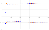
Figure 8: Values of $y$ such that the unitary integral yields the same value as the orthogonal one.

Remark.

For reference, the solutions for $y$ for odd and even dimensions are plotted in Fig. (8).

B3. Maximization and minimization of the fourth moment $\mathcal{S}_{AB}^{(4)}$

Let us discuss the maximization and minimization of the fourth moment $\mathcal{S}_{AB}^{(4)}$ for separable states, which leads to the area plotted in Fig. 2. As we described in the main text, the moments $\mathcal{S}^{(r)}_{AB}$ are, by definition, invariant under orthogonal transformations of the submatrix $T_{\mathrm{s}}$, where $T_{\mathrm{s}}=(t_{ij})$ with $1\leq i,j\leq d^{2}-1$ in Eq. (8). This orthogonal invariance allows us to consider the diagonalization of the submatrix $T_{\mathrm{s}}$

$$T_{\mathrm{s}}^{\prime}=O_{A}T_{\mathrm{s}}O_{B}^{\top}=\mathrm{diag}(\tau_{1},\tau_{2},\ldots,\tau_{d^{2}-1}),$$ (S.99)

where $O_{A},O_{B}\in SO(d^{2}-1)$ are non-physical orthogonal matrices and $\tau_{i}\geq 0$ are singular values of $T_{\mathrm{s}}$. With this, we are able to reduce the number of parameters for the moments $\mathcal{S}^{(r)}_{AB}$. In fact, the evaluated second and fourth moments (S.52, S.53) can be simply expressed as

$$\mathcal{S}^{(2)}_{AB} =V\sum_{i=1}^{d^{2}-1}\tau_{i}^{2},$$ (S.100)

$$\mathcal{S}^{(4)}_{AB} =W\left[2\sum_{i=1}^{d^{2}-1}\tau_{i}^{4}+\left(\sum_{i=1}^{d^{2}-1}\tau_{i}^{2}\right)^{2}\right]=W\left[2\sum_{i=1}^{d^{2}-1}\tau_{i}^{4}+\frac{1}{V^{2}}\left(\mathcal{S}^{(2)}_{AB}\right)^{2}\right],$$ (S.101)

where $V=1/(d-1)^{2}$ and $W=1/3(d-1)^{4}$. To maximize and minimize the fourth moment $\mathcal{S}^{(4)}_{AB}$, we fix the second moment $\mathcal{S}^{(2)}_{AB}$ and employ the dV criterion as the constraint:

$$\|T_{\mathrm{s}}\|_{\text{tr}}=\|T_{\mathrm{s}}^{\prime}\|_{\text{tr}}=\sum_{i=1}^{d^{2}-1}\tau_{i}\leq d-1.$$ (S.102)

Then the task reads

$$\max_{\tau_{i}}/\min_{\tau_{i}}\ \ \ \ \ \ \ \ \ \ \ \ \ \ \ \mathcal{S}^{(4)}_{AB} =W\left[2\sum_{i=1}^{d^{2}-1}\tau_{i}^{4}+\frac{1}{V^{2}}\left(\mathcal{S}^{(2)}_{AB}\right)^{2}\right],$$ (S.103)

$$\mathrm{s.t.}\ \ \ \ \ \ \ \ \ \ \ \ \ \ \ \ \,\ \ \ \ \ \ \ \mathcal{S}^{(2)}_{AB} =V\sum_{i=1}^{d^{2}-1}\tau_{i}^{2},$$ (S.104)

$$\sum_{i=1}^{d^{2}-1}\tau_{i} \leq d-1,$$ (S.105)

$$0 \leq\tau_{i}\leq d-1,$$ (S.106)

where $\tau_{i}$ is maximal and equal to $d-1$ for a pure product state, due to the positivity of states. Consequently, we can characterize the set of admissible values $\left(\mathcal{S}^{(2)}_{AB},\,\mathcal{S}^{(4)}_{AB}\right)$ for separable states by maximizing and minimizing the fourth moment. If a state lies outside this set, then it must be entangled.

The lower bound for PPT states can be obtained by numerical optimization. Also, the lower bound for general states can be obtained by imposing the constraint $\sum_{i=1}^{d^{2}-1}\tau_{i}\leq d^{2}-1$, and the isotropic state $\varrho_{\mathrm{iso}}$ in Eq. (S.51) satisfies the bound, which proves it is optimal.

In the main text, we showed the zoom-in plot in Fig. 2. Here, we also give the zoom-out plot in Fig. 9. Moreover, for reference, the results for $d=4$ are shown in Fig. 10. Importantly, the $4\otimes 4$ bound entangled Piani state from the Refs. [57] is outside of the region of separable states, meaning that it can be detected by the method of moments with random correlations developed in this paper.

Let us discuss which states are good candidates for violating our criterion. It is known that in $d\otimes d$-dimensional systems, if the states have maximally mixed subsystems, then the dV criterion is equivalent to the CCNR criterion. If not, the dV criterion is weaker than the CCNR criterion (see Ref. [58]). On the other hand, if an entangled state is very closed to a state with maximally mixed subsystems and largely violates the CCNR criterion, then we may detect the entangled state based on the dV criterion. For instance, the so-called cross-hatch $3\times 3$ grid state, one of the bound entangled states detected by our methods, does not have maximally mixed subsystems. Nevertheless, its reduced states is close to maximally mixed, $\rho_{A}=\rho_{B}=\text{diag}(0.375,0.25,0.375)$, and moreover, it violates the CCNR criterion by a large amount.

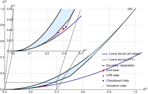
Figure 9: Entanglement criterion based on second and fourth moments of randomized measurements for $3\otimes 3$ systems.

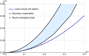
Figure 10: Entanglement criterion based on second and fourth moments of randomized measurements for $4\otimes 4$ systems. The bound entangled state is outside, meaning that it can be detected with the methods developed in this paper.

Appendix C: Bound entangled states

In Appendix C, we give explicit forms of the bound entangled states that can be detected by the methods with randomized measurements: (1) quantum grid states (2) chessboard states (3) states forming unextendible product bases (4) $3\otimes 3$ Horodecki state (5) the $4\otimes 4$ bound entangled Piani state. We remark that Yu-Oh bound entangled states [59] and steering bound entangled states [74] cannot be detected by our methods.

C1. Quantum grid states

A quantum grid state is a toy model that can describe the mixture of entangled states. Its entanglement properties have been characterized using entanglement criteria [76]. For $d\otimes d$-dimensional systems, consider a pure entangled state forming

$$\ket{i,j;k,l}=\frac{1}{\sqrt{2}}\left(\ket{ij}-\ket{kl}\right),$$ (S.107)

with $0\leq i,j,k,l<d$. A quantum $d\times d$ grid state is defined as the uniform mixture of pure states $\ket{i,j;k,l}$. That is, for a given set $E=\{\ket{i,j;k,l}\}$, it can be defined as

$$\varrho(E)=\frac{1}{|E|}\sum_{\ket{e}\in E}\ket{e}\!\bra{e}.$$ (S.108)

Note that not all quantum grid states are separable, and moreover, there are some grid states that can have bound entanglement. In particular, a $3\times 3$ bound entangled grid state is called the cross-hatch state with the set $E_{\mathrm{ch}}=\{\ket{1,1;2,3},\ket{2,1;3,3},\ket{1,2;3,1},\ket{1,3;3,2}\}$, see also Fig. 2 (a) in [76]. It is known that the cross-hatch state is detected by the CCNR criterion.

C2. Chessboard states

For $3\otimes 3$-dimensional systems, consider a family of quantum states

$$\varrho_{\mathrm{cb}}=N\sum_{i=1}^{4}\ket{V_{i}}\!\bra{V_{i}},$$ (S.109)

where $N=1/\sum_{i}\Braket{V_{i}}{V_{i}}$ is a normalization factor and

$$\ket{V_{1}} =(m,0,s;0,n,0;0,0,0),$$ (S.110)

$$\ket{V_{2}} =(0,a,0;b,0,c;0,0,0),$$ (S.111)

$$\ket{V_{3}} =(n,0,0;0,-m,0;t,0,0),$$ (S.112)

$$\ket{V_{4}} =(0,b,0;-a,0,0;0,d,0).$$ (S.113)

with free real parameters $a,b,c,d,m,n$ and $s=\frac{ac}{n},t=\frac{ad}{m}$. The matrix form of this state can then be expressed as

$$\varrho_{\mathrm{cb}}=\begin{pmatrix}m^{2}+n^{2}&0&ms&0&0&0&nt&0&0\\ 0&a^{2}+b^{2}&0&0&0&ac&0&bd&0\\ sm&0&s^{2}&0&sn&0&0&0&0\\ 0&0&0&a^{2}+b^{2}&0&bc&0&-ad&0\\ 0&0&ns&0&m^{2}+n^{2}&0&-mt&0&0\\ 0&ac&0&cb&0&c^{2}&0&0&0\\ tn&0&0&0&-tm&0&t^{2}&0&0\\ 0&bd&0&-da&0&0&0&d^{2}&0\\ 0&0&0&0&0&0&0&0&0\\ \end{pmatrix}.$$ (S.114)

The states $\varrho_{\mathrm{cb}}$ are called the chessboard states because their $8\times 8$ matrix form looks like a chessboard, originally introduced by Dagmar Bruß and Asher Peres [77]. The state $\varrho_{\mathrm{cb}}$ is invariant under the partial transposition: $\varrho_{\mathrm{cb}}=\varrho_{\mathrm{cb}}^{T_{B}}\geq 0$. On the other hand, according to the range criterion [60], $\varrho_{\mathrm{cb}}$ is entangled. Thus, the chessboard states are bound entangled. The extremal PPT entangled state shown in Fig. 2 in the main text and Fig. 9 is a state from this family with $m=n=b=-3/5$, $a=3/5$, $c=-d=6/5$.

C3. Unextendible product bases

For $3\otimes 3$-dimensional systems, consider five product states

$$\ket{\psi_{0}} =\frac{1}{\sqrt{2}}\ket{0}(\ket{0}-\ket{1}),\ \ \ \ \ \ket{\psi_{1}}=\frac{1}{\sqrt{2}}(\ket{0}-\ket{1})\ket{2},\ \ \ \ \ \ket{\psi_{2}}=\frac{1}{\sqrt{2}}\ket{2}(\ket{1}-\ket{2}),$$ (S.115)

$$\ket{\psi_{3}} =\frac{1}{\sqrt{2}}(\ket{1}-\ket{2})\ket{0},\ \ \ \ \ \ket{\psi_{4}}=\frac{1}{3}(\ket{0}+\ket{1}+\ket{2})(\ket{0}+\ket{1}+\ket{2}).$$ (S.116)

Notice that all of these five product states are orthogonal to all pairs, and another product state cannot be orthogonal to all pairs. These product states are said to form an unextendible product basis (UPB) [78]. From these states, one can construct the mixed state

$$\varrho_{\mathrm{UPB}}=\frac{1}{4}\left(\mathbbm{1}-\sum_{i=0}^{4}\ket{\psi_{i}}\!\bra{\psi_{i}}\right).$$ (S.117)

Here, $\varrho_{\mathrm{UPB}}$ is the state on the space that is orthogonal to the space spanned by the UPB. Then, $\varrho_{\mathrm{UPB}}$ has no product states in the range. According to the range criterion [60], $\varrho_{\mathrm{UPB}}$ should be entangled. On the other hand, one can notice that $\varrho_{\mathrm{UPB}}$ is invariant under the partial transposition: $\varrho_{\mathrm{UPB}}^{T_{B}}=\varrho_{\mathrm{UPB}}\geq 0$. Hence, $\varrho_{\mathrm{UPB}}$ is a bound entangled state.

C4. $3\otimes 3$ Horodecki state

For $3\otimes 3$-dimensional systems, consider the mixed state

$$\sigma(p)=\frac{2}{7}\ket{\psi^{+}}\!\bra{\psi^{+}}+\frac{p}{7}\sigma_{+}+\frac{5-p}{7}\sigma_{-},\ \ \ \ \ \ \ 2\leq p\leq 5,$$ (S.118)

where

$$\ket{\psi^{+}} =\frac{1}{\sqrt{3}}(\ket{00}+\ket{11}+\ket{22}),$$ (S.119)

$$\sigma_{+} =\frac{1}{3}(\ket{01}\!\bra{01}+\ket{12}\!\bra{12}+\ket{20}\!\bra{20}),$$ (S.120)

$$\sigma_{-} =\frac{1}{3}(\ket{10}\!\bra{10}+\ket{21}\!\bra{21}+\ket{02}\!\bra{02}).$$ (S.121)

It turns out that the state $\sigma(p)$ is PPT in the range $2\leq p\leq 4$. To characterize this state further, one can employ a non-decomposable positive map $\Lambda$ such that $(\mathbbm{1}\otimes\Lambda)\sigma\ngeq 0$. An example is

$$\Lambda\begin{pmatrix}a_{11}&a_{12}&a_{13}\\ a_{21}&a_{22}&a_{23}\\ a_{31}&a_{32}&a_{33}\\ \end{pmatrix}=\begin{pmatrix}a_{11}&-a_{12}&-a_{13}\\ -a_{21}&a_{22}&-a_{23}\\ -a_{31}&-a_{32}&a_{33}\\ \end{pmatrix}+\begin{pmatrix}a_{22}&0&0\\ 0&a_{33}&0\\ 0&0&a_{11}\\ \end{pmatrix}.$$ (S.122)

This non-decomposable map allows us to classify this state as follows [79]: the state $\sigma(p)$ is not detected as entangled for $2\leq p\leq 3$, PPT (bound) entangled for $3<p\leq 4$, and NPT entangled for $4<p\leq 5$.

C5. $4\otimes 4$ bound entangled Piani state

For $4\otimes 4$-dimensional systems, consider the orthogonal projections

$$P_{ij}=\ket{{\Psi_{ij}}}\!\bra{{\Psi_{ij}}},$$ (S.123)

where $\ket{{\Psi_{ij}}}=(\mathbbm{1}\otimes\sigma_{ij})\ket{\Psi_{+}^{4}}$, $\ket{\Psi_{+}^{4}}=\frac{1}{2}\sum_{k=0}^{3}\ket{kk}$, and $\sigma_{ij}=\sigma_{i}\otimes\sigma_{j}$ with Pauli matrices. With these projections, one can construct the state

$$\varrho_{\mathrm{BE}} =\frac{1}{6}\left(P_{02}+P_{11}+P_{23}+P_{31}+P_{32}+P_{33}\right)$$ (S.124)

$$=\frac{1}{6}\left(\Phi^{+}_{AB}\Psi^{-}_{A^{\prime}B^{\prime}}+\Psi^{+}_{AB}\Psi^{+}_{A^{\prime}B^{\prime}}+\Psi^{-}_{AB}\Phi^{-}_{A^{\prime}B^{\prime}}+\Phi^{-}_{AB}\Psi^{+}_{A^{\prime}B^{\prime}}+\Phi^{-}_{AB}\Psi^{-}_{A^{\prime}B^{\prime}}+\Phi^{-}_{AB}\Phi^{-}_{A^{\prime}B^{\prime}}\right),$$ (S.125)

where $\Phi^{+},\Phi^{-},\Psi^{+},\Psi^{-}$ are also projectors on the Bell states. It has been shown that the state $\varrho_{\mathrm{BE}}$ is the $4\otimes 4$ bound entangled under the bipartition of $AA^{\prime}|BB^{\prime}$ [57].

Appendix D: Numerical methods

In Appendix D, we provide numerical methods to check the results presented in the main text. Indeed, our conjecture that Observation 2 holds for mixtures of product states with different bipartitions, as well as the PPT boundary in Fig. 2 are obtained by extensive numerical searches. These are performed using Python and the optimization functions of the package SciPy [61].

In particular, when optimizing over mixed separable states to check Observation 2, we parametrize these states for a fixed rank $r$ by constructing $r$ unnormalized pure product states w.r.t. different bipartitions. We mix these states and rescale the result to form a proper quantum state. The actual optimization is then performed using the BFGS algorithm [41, 42, 43, 44], implemented in SciPy. We ran the optimization for different values of $r$ up to $r=8$, and all possible choices of the bipartitions. In order to minimize the risk of getting stuck in local minima, we repeated each of the optimizations $50$ times with random initial parameters.

In order to obtain the PPT bound in Fig. 2, we parametrize the random density matrices by rearranging the variables into a hermitian matrix, then form the normalized square of it to obtain a proper quantum state. We then minimize its fourth moment for different constant values of the second moment with the constraint that its partial transpose is positive. These constraints are implemented via penalty terms in the target function. We then sampled the range of the second moment and ran the optimization $10$ times for each value, to reduce the risk of being stuck in a local minimum.

The source code for these optimizations is available upon reasonable request.

References

[1]
J. Emerson, R. Alicki, and K. Życzkowski,
J. Opt. B: Quantum Semiclassical Opt. 7, S347 (2005).
[2]
E. Knill, D. Leibfried, R. Reichle, J. Britton, R. B. Blakestad, J. D. Jost,
C. Langer, R. Ozeri, S. Seidelin, and D. J. Wineland,
Phys. Rev. A 77, 012307 (2008).
[3]
S. T. Flammia and Y.-K. Liu,
Phys. Rev. Lett. 106, 230501 (2011).
[4]
S. Aaronson,
Proc. Roy. Soc. London A 463,
3089 (2007).
[5]
H.-Y. Huang, R. Kueng, and J. Preskill,
Nature Phys. 16, 1050 (2020).
[6]
J. Morris and B. Dakić,
arXiv:1909.05880.
[7]
F.G.S.L. Brandão, R. Kueng, and D. Stilck França,
arXiv:2009.08216.
[8]
Y.-C. Liang, N. Harrigan, S. D. Bartlett, and T. Rudolph,
Phys. Rev. Lett. 104, 050401 (2010).
[9]
J. J. Wallman and S. D. Bartlett,
Phys. Rev. A 85, 024101 (2012).
[10]
P. Shadbolt, T. Vertesi, Y.-C. Liang, C. Branciard, N. Brunner, J. L. OB́rien,
Scientific Reports 2, 470 (2012).
[11]
S. D. Bartlett, T. Rudolph, and R. W. Spekkens,
Phys. Rev. Lett. 91, 027901 (2003).
[12]
S. D. Bartlett, T. Rudolph, and R. W. Spekkens,
Rev. Mod. Phys. 79, 555 (2007).
[13]
A. Laing, V. Scarani, J. G. Rarity, and J. L. OB́rien,
Phys. Rev. A 82, 012304 (2010).
[14]
P. Hayden, S. Nezami, S. Popescu, and G. Salton,
PRX Quantum 2, 010326 (2021).
[15]
S. J. van Enk and C. W. J. Beenakker,
Phys. Rev. Lett. 108, 110503 (2012).
[16]
A. Elben, B. Vermersch, M. Dalmonte, J. I. Cirac, and P. Zoller,
Phys. Rev. Lett. 120, 050406 (2018).
[17]
T. Brydges, A. Elben, P. Jurcevic, B. Vermersch, C. Maier, B. P. Lanyon, P. Zoller, R. Blatt, and C. F. Roos,
Science 364, 260 (2019).
[18]
A. Peres,
Phys. Rev. Lett. 77, 1413 (1996).
[19]
M. Horodecki, P. Horodecki, and R. Horodecki,
Phys. Lett. A 223, 1 (1996).
[20]
Y. Zhou, P. Zeng, and Z. Liu,
Phys. Rev. Lett. 125, 200502 (2020).
[21]
A. Elben, R. Kueng, H.-Y. Huang, R. van Bijnen, C. Kokail, M. Dalmonte, P. Calabrese, B. Kraus, J. Preskill, P. Zoller, and B. Vermersch,
Phys. Rev. Lett. 125, 200501 (2020).
[22]
M. C. Tran, B. Dakić, F. Arnault, W. Laskowski, and T. Paterek,
Phys. Rev. A 92, 050301 (2015).
[23]
M. C. Tran, B. Dakić, W. Laskowski, and T. Paterek,
Phys. Rev. A 94, 042302 (2016).
[24]
L. Knips, J. Dziewior, W. Kłobus, W. Laskowski, T. Paterek, P. J. Shadbolt, H. Weinfurter, J. D. A. Meinecke,
npj Quantum Inf. 6, 51 (2020).
[25]
A. Ketterer, N. Wyderka, and O. Gühne,
Phys. Rev. Lett. 122, 120505 (2019).
[26]
A. Ketterer, S. Imai, N. Wyderka, and O. Gühne,
arXiv:2012.12176.
[27]
A. Ketterer, N. Wyderka, and O. Gühne,
Quantum 4, 325 (2020).
[28]
L. Knips,
Quantum Views 4, 47 (2020).
[29]
O. Rudolph,
Quantum Inf. Proc. 4, 219 (2005);
see also e-print quant-ph/0202121.
[30]
K. Chen and L.-A. Wu,
Quant. Inf. Comp. 3, 193 (2003).
[31]
J. I. de Vicente,
Quantum Inf. Comput. 7, 624 (2007).
[32]
C. Dankert,
M.Math. thesis, University of Waterloo (2005);
also available as e-print quant-ph/0512217.
[33]
H. Aschauer, J. Calsamiglia, M. Hein, and H. J. Briegel,
Quant. Inf. Comp. 4, 383 (2004).
[34]
J. I. de Vicente and M. Huber,
Phys. Rev. A 84, 062306 (2011).
[35]
C. Klöckl and M. Huber,
Phys. Rev. A 91, 042339 (2015).
[36]
N. Wyderka and O. Gühne,
J. Phys. A: Math. Theor. 53, 345302 (2020).
[37]
C. Eltschka and J. Siewert,
Quantum 4, 229 (2020).
[38]
F. Mintert, M. Kuś, and A. Buchleitner,
Phys. Rev. Lett. 95, 260502 (2005).
[39]
L. Aolita, A. Buchleitner, and F. Mintert,
Phys. Rev. A 78, 022308 (2008).
[40]
See Supplemental Material for the appendices
which include Refs. [41-61].
[41]
C. G. Broyden, IMA J. Appl. Math. 6,
222 (1970).
[42]
R. Fletcher,
Comput. J. 13,
317 (1970).
[43]
D. Goldfarb,
Math. Comput.
24,
23 (1970).
[44]
D. F. Shanno,
Math. Comput. 24,
647 (1970).
[45]
R. Lohmayer, A. Osterloh, J. Siewert, and A. Uhlmann,
Phys. Rev. Lett. 97, 260502 (2006).
[46]
S. Szalay,
Phys. Rev. A 83, 062337 (2011).
[47]
M. Huber, F. Mintert, A. Gabriel, and B. C. Hiesmayr,
Phys. Rev. Lett. 104, 210501 (2010).
[48]
W. Dür, J. I. Cirac, and R. Tarrach,
Phys. Rev. Lett. 83, 3562 (1999).
[49]
Z. -H. Chen, Z. -H. Ma, O. Gühne, and S. Severini,
Phys. Rev. Lett. 109, 200503 (2012).
[50]
O. Gühne, M. Seevinck,
New J. Phys. 12, 053002 (2010).
[51]
B. Jungnitsch, T. Moroder, and O. Gühne,
Phys. Rev. Lett. 106, 190502 (2011).
[52]
P. Rungta, V. Bužek, C. M. Caves, M. Hillery, and G. J. Milburn,
Phys. Rev. A 64, 042315 (2001).
[53]
C. Eltschka and J. Siewert,
Quantum 2, 64 (2018).
[54]
G. B. Folland,
Am. Math. Mon 108, 446 (2001).