Multi-fidelity data fusion for the approximation of scalar functions with low intrinsic dimensionality through active subspaces

Abstract

Gaussian processes are employed for non-parametric regression in a Bayesian setting. They generalize linear regression embedding the inputs in a latent manifold inside an infinite-dimensional reproducing kernel Hilbert space. We can augment the inputs with the observations of low-fidelity models in order to learn a more expressive latent manifold and thus increment the model’s accuracy. This can be realized recursively with a chain of Gaussian processes with incrementally higher fidelity. We would like to extend these multi-fidelity model realizations to case studies affected by a high-dimensional input space but with low intrinsic dimensionality. In these cases physical supported or purely numerical low-order models are still affected by the curse of dimensionality when queried for responses. When the model’s gradient information is provided, the presence of an active subspace can be exploited to design low-fidelity response surfaces and thus enable Gaussian process multi-fidelity regression, without the need to perform new simulations. This is particularly useful in the case of data scarcity. In this work we present a multi-fidelity approach involving active subspaces and we test it on two different high-dimensional benchmarks.

lox

1 Introduction

Every day more and more complex simulations are made possible thanks to the high-performance computing facilities spread and to the advancements in computational methods. Still the study and the approximation of high-dimensional functions of interest represent a problem due to the curse of dimensionality and the data scarcity because of limited computation budgets.

Gaussian processes (GP) [42] have been proved as a versatile and powerful technique for regression (GPR), classification, inverse problem resolution, and optimization, among others. In the last years several studies and extensions have been proposed in the context of non-parametric and interpretable Bayesian models. For a review on Gaussian processes and kernel methods we suggest [14], while for approximation methods in the framework of GP see [27]. Progress has also been made to deal with big data and address some memory limitations of GPR, as for example by sparsifying the spectral representation of the GP [18] or introducing stochastic variational inference for GP models [21].

Multi-fidelity modelling has been proven effective in a heterogeneous set of applications [15, 11, 28, 2, 3, 16], where expensive but accurate high-fidelity measurements are coupled with cheaper to compute and less accurate low-fidelity data. Recent advancements have been made for nonlinear autoregressive multi-fidelity Gaussian process regression (NARGP) as proposed in [26], and with physics informed neural networks (PINNs) [29] in the context of multi-fidelity approximation in [23].

The increased expressiveness of these models is achieved thanks to some kind of nonlinear approach that extend GP models to non-GP processes with the disadvantage of an additional computational cost. In this direction are focused the following works which aim to obtain computationally efficient heteroscedastic GP models with a variational inference approach [19] or employing a nonlinear transformation [35]. This approach is extended to multi-fidelity models departing from the linear formulation of Kennedy and O’Hagan [15] towards deep Gaussian processes [6] and NARPG.

When the models depend on a high-dimensional input space even the low-fidelity approximations supported by a physical interpretation or a purely numerical model order reduction suffer from the curse of dimensionality especially for the design of high-dimensional GP models. Active subspaces (AS) [4, 43] can be used to build a surrogate low-fidelity model with reduced input space taking advantage of the correlations of the model’s gradients when available. Reduction in parameter space through AS has been proven successful in a diverse range of applications such as: shape optimization [22, 9], hydrologic models [13], naval and nautical engineering [41, 7, 24, 37, 39], coupled with intrusive reduced order methods in cardiovascular studies [36], in CFD problems in a data-driven setting [8, 40]. A kernel-based extension of AS for both scalar and vectorial functions can be found in [30].

The aim of the present contribution is to propose a multi-fidelity regression model which exploits the intrinsic dimensionality of high-dimensional functions of interest and the presence of an active subspace to reduce the approximation error of high-fidelity response surfaces. Our approach employs the design of a NARGP using an AS response surface as low-fidelity model. In the literature the multi-fidelity approximation paradigm has been adopted in a different way to search for an active subspace from given high- and low-fidelity models [17].

The outline of this work is the following: in Section 2 we present the general framework of Gaussian process regression and in particular the NARGP multi-fidelity approach; in Section 3 we briefly present the Active subspaces property we are going to exploit as low-fidelity model, together with some error estimates for the construction of response surfaces; Section 4 is devoted to present how data fusion with Active subspaces is performed with the aid of algorithms; in Section 5 we apply the proposed approach to the piston and Ebola benchmark models showing the better performance achieved by the multi-fidelity regression; finally in Section 6 we present our conclusions and we draw some future perspectives.

2 Multi-fidelity Gaussian process regression

In the next subsections we are going to present the Gaussian process regression (GPR) [42] technique which is the building block of multi-fidelity GPR, and the nonlinear autoregressive multi-fidelity Gaussian process regression (NARGP) [26] we are going to use in this work. The numerical methods are presented for the general case of several levels of fidelity.

2.1 Gaussian process regression

Gaussian process regression [42] is a supervised technique to approximate unknown functions given a finite set of input/output pairs $\mathcal{S}=\{x_{i},y_{i}\}_{i=1}^{N}$. Let $f:\mathcal{X}\subset\mathbb{R}^{D}\to\mathbb{R}$ be the scalar function of interest. The set $\mathcal{S}$ is generated through $f$ with the following relation: $y_{i}=f(x_{i})$, which are the noise-free observations. To $f$ is assigned a prior with mean $m(\mathbf{x})$ and covariance function $k(\mathbf{x},\mathbf{x}^{\prime};\theta)$, that is $f(\mathbf{x})\sim\mathcal{GP}(m(\mathbf{x}),k(\mathbf{x},\mathbf{x}^{\prime};\theta))$. The prior expresses our beliefs about the function before looking at the observed values. From now on we consider zero mean $\mathcal{GP}$, $m(\mathbf{x})=\mathbf{0}$, and we define the covariance matrix $\mathbf{K}_{i,j}=k(x_{i},x_{j};\theta)$, with $\mathbf{K}\in\mathbb{R}^{N\times N}$. To use the Gaussian process to make prediction we still need to find the optimal values of the elements of the hyper-parameters vector $\theta$. We achieve this by maximizing the log marginal likelihood:

$$\log p(\mathbf{y}|\mathbf{x},\theta)=-\frac{1}{2}\mathbf{y}^{T}\mathbf{K}^{-1}\mathbf{y}-\frac{1}{2}\log|\mathbf{K}|-\frac{N}{2}\log 2\pi.$$ (1)

Let $\mathbf{x}_{*}$ be the test samples, and $\mathbf{K}_{N*}=k(\mathbf{x},\mathbf{x}_{*};\theta)$ be the matrix of the covariances evaluated at all pairs of training and test samples, and in a similar fashion $\mathbf{K}_{*N}=k(\mathbf{x}_{*},\mathbf{x};\theta)$, and $\mathbf{K}_{**}=k(\mathbf{x}_{*},\mathbf{x}_{*};\theta)$. By conditioning the joint Gaussian distribution on the observed values we obtain the predictions $f_{*}$ by sampling the posterior

$$f_{*}|\mathbf{x}_{*},\mathbf{x},\mathbf{y}\sim\mathcal{N}(\mathbf{K}_{*N}\mathbf{K}^{-1}\mathbf{y},\mathbf{K}_{**}-\mathbf{K}_{*N}\mathbf{K}^{-1}\mathbf{K}_{N*}).$$ (2)

2.2 Nonlinear multi-fidelity Gaussian process regression

We adopt the nonlinear autoregressive multi-fidelity Gaussian process regression (NARGP) scheme proposed in [26]. It extends the concepts present in [15, 20] to nonlinear correlations between the different fidelities available.

We introduce $p$ levels of increasing fidelities and the corresponding sets of input/output pairs $\mathcal{S}_{q}=\{x_{i}^{q},y_{i}^{q}\}_{i=1}^{N_{q}}\subset\mathcal{X}\times\mathbb{R}\subset\mathbb{R}^{n}\times\mathbb{R}$ for $q\in\{1,\dots,p\}$, where $y_{i}^{q}=f_{q}(x_{i}^{q})$. With $p$ we indicate the highest fidelity. We also assume the design sets to have a nested structure: $\mathcal{S}_{p}\subset\mathcal{S}_{p-1}\subset\cdots\subset\mathcal{S}_{1}$.

The NARGP formulation considers the following autoregressive multi-fidelity scheme:

$$f_{q}(\mathbf{x})=g_{q}(\mathbf{x},f_{*q-1}(\mathbf{x})),$$ (3)

where $f_{*q-1}(\mathbf{x})$ is the GP posterior from the previous inference level $q-1$, and to $g_{q}$ is assigned the following prior:

$$g_{q} \sim\mathcal{GP}(f_{q}|\mathbf{0},k_{q};\theta_{q})$$ (4)

$$k_{q} =k_{q}^{\rho}(\mathbf{x},\mathbf{x}^{\prime};\theta_{q}^{\rho})\cdot k_{q}^{f}(f_{*q-1}(\mathbf{x}),f_{*q-1}(\mathbf{x}^{\prime});\theta_{q}^{f})+k_{q}^{\delta}(\mathbf{x},\mathbf{x}^{\prime};\theta_{q}^{\delta}),$$ (5)

with $k_{q}^{\rho}$, $k_{q}^{f}$, and $k_{q}^{\delta}$ squared exponential kernel functions. With this scheme, through $g_{q}$ we can infer the high-fidelity response by projecting the lower fidelity posterior to a latent manifold of dimension $D+1$. This structure allows for nonlinear and more general cross-correlations between subsequent fidelities.

A part from the first level of fidelity $q=1$ the posterior probability distribution given the previous fidelity models is no longer Gaussian since the inputs are couples $((\mathbf{x},\mathbf{x}_{*}),(y_{q-1}(\mathbf{x}),f_{*q-1}(\mathbf{x}_{*}))$ where $f_{q-1}$ is a Gaussian process $g_{q}\sim\mathcal{GP}(f_{q}|\mathbf{0},k_{q};\theta_{q})$, the training set is $(\mathbf{x},f_{q-1}(\mathbf{x}))$ and $\mathbf{x}_{*}$ is the new input. So in order to evaluate the predictive mean and variance for a new input $\mathbf{x}_{*}$ we have to integrate the usual Gaussian posterior $p(f_{*q}(\mathbf{x}_{*},f_{*q-1}(\mathbf{x}_{\star}))|f_{*q-1},\mathbf{x}_{*},\mathbf{x}_{q},\mathbf{y}_{q})$ explicited as

$$f_{*q}(\mathbf{x}_{*},f_{*q-1}(\mathbf{x}_{\star}))|f_{*q-1},\mathbf{x}_{*},\mathbf{x}_{q},\mathbf{y}_{q}\sim\mathcal{N}(\mathbf{K}^{q}_{*N}(\mathbf{K}^{q})^{-1}y_{q},\mathbf{K}^{q}_{**}-\mathbf{K}^{q}_{*N}(\mathbf{K}^{q})^{-1}\mathbf{K}^{q}_{N*}),$$ (6)

$$K_{*N}^{q}=k_{q}((\mathbf{x}_{*},f_{*q-1}(\mathbf{x}_{*}),(\mathbf{x}_{q-1},y_{q-1});\theta),$$ (7)

$$K_{N*}^{q}=k_{q}((\mathbf{x}_{q-1},y_{q-1}),(\mathbf{x}_{*},f_{*q-1}(\mathbf{x}_{*});\theta),$$ (8)

$$K^{q}=k_{q}((\mathbf{x}_{q-1},y_{q-1}),(\mathbf{x}_{q-1},y_{q-1});\theta),$$ (9)

over the Gaussian distribution of the prediction at the previous level $f_{*q-1}(\mathbf{x}_{*})\sim\mathcal{N}(\mu_{x_{*}},\sigma_{\mathbf{x}_{*}})$. In practice the following integral is approximated with recursive Monte Carlo in each fidelity level

$$p(f_{*q}(\mathbf{x}_{*},f_{*q-1}(\mathbf{x}_{*})))=\int_{\mathcal{X}}p(f_{*q}(\mathbf{x}_{*},f_{*q-1}(\mathbf{x}_{*}))|f_{*q-1},\mathbf{x}_{*},\mathbf{x}_{q},\mathbf{y}_{q})p(f_{*q-1}(\mathbf{x}_{*}))d\mathbf{x}_{*}.$$ (10)

3 Active subspaces property

In this section we follow the work of P.G. Constantine [4]. Our aim is testing multi-fidelity Gaussian process regression models to approximate objective functions which depend on inputs sampled from a high-dimensional space. Low-fidelity models relying on a physical supported or numerical model reduction (for example a coarse discretization or a more specific numerical model order reduction) still suffer from the high dimensionality of the input space.

In our approach we try to tackle these problematics by searching for a surrogate (low-fidelity) model accounting for the complex correlations among the input parameters that concur to the output of interest. With this purpose in mind we query the model for an active subspace and employing the found active subspace we design a response surface with Gaussian process regression.

3.1 Response surface design with active subspaces

Let us suppose the inputs are represented by an absolutely continuous random variable $\mathbf{X}$ with probability density $\rho$ such that $\text{supp}(\rho)=\mathcal{X}\subset\mathbb{R}^{m}$ where $m$ is the dimension of the input space. If our numerical simulations provide also the gradients of the samples for which the model is inquired for, we can approximate the correlation matrix of the gradient with simple Monte Carlo as

$$\mathbb{E}_{\rho}[\nabla_{\mathbf{x}}f(\nabla_{\mathbf{x}}f)^{T}]\approx\frac{1}{N}\sum_{i=1}^{N}\nabla_{\mathbf{x}}f(\mathbf{X}_{i})(\nabla_{\mathbf{x}}f(\mathbf{X}_{i}))^{T},$$ (11)

where $N$ is the number of sampled inputs. We then search for the highest spectral gap $\lambda_{r}-\lambda_{r+1}$ in the sequence of ordered eigenvalues of the approximated correlation matrix

$$\lambda_{1}\geq\dots\geq\lambda_{r}\geq\lambda_{r+1}\geq\dots\geq\lambda_{m}.$$ (12)

The active subspace is the eigenspace corresponding to the eigenvalues $\lambda_{1},\dots,\lambda_{r}$ and we represent it with the matrix $\hat{W}_{1}\in\mathcal{M}(m\times r)$ which columns are the first $r$ active eigenvectors. Then the response surface $\mathcal{R}$ is built with a Gaussian process regression over the training set composed by $N_{\text{train}}$ input-output pairs $\{W_{1}^{T}\mathbf{x}_{i},y_{i}\}_{i=1}^{N_{\text{train}}}$.

An a priori bound on the error can be proved [4], but the whole approximation procedure considers additional steps for the evaluation of the optimal profile $\mathbb{E}_{\rho}[f|\hat{W}_{1}^{T}\mathbf{X}]$ and its approximation with Monte Carlo $\overline{\mathbb{E}_{\rho}[f|\hat{W}_{1}^{T}\mathbf{X}]}$,

$$f(\mathbf{X})\approx\mathbb{E}_{\rho}[f|\hat{W}_{1}^{T}\mathbf{X}]\approx\overline{\mathbb{E}_{\rho}[f|\hat{W}_{1}^{T}\mathbf{X}]}\approx\mathcal{R}(\hat{W}_{1}\mathbf{X}).$$ (13)

The mean square regression error is bounded a-priori by,

$$\mathbb{E}_{\rho} \left[(f(\mathbf{X})-\mathcal{R}(\hat{W}_{1}^{T}\mathbf{X}))^{2}\right]$$

$$\leq\ C_{1}(1+N^{-1/2})^{2}\left(\epsilon(\lambda_{1}+\dots+\lambda_{r})^{1/2}+(\lambda_{r+1}+\dots+\lambda_{m})^{1/2}\right)^{2}+C_{2}\delta,$$

where $C_{1}$ and $C_{2}$ are constants, $\epsilon$ quantifies the error in the approximation of the true active subspace $W_{1}$ with $\hat{W}_{1}$ obtained from the Monte Carlo approximation and $C_{2}\delta$ is a uniform bound on

$$\mathbb{E}_{\rho}[\overline{(\mathbb{E}_{\rho}[f|\hat{W}_{1}^{T}\mathbf{X}]}-\mathcal{R}(\hat{W}_{1}^{T}\mathbf{X})^{2}|W_{2}^{T}\mathbf{X}]\leq C_{2}\delta.$$ (14)

4 Multi-fidelity data fusion with active subspaces

Our study is based on the design of a nonlinear autoregressive multi-fidelity Gaussian process regression (NARGP) [26] whose low-fidelity level is learnt from a response surface built through the active subspaces methodology. In fact we suppose that the model in consideration has indeed a high dimensional input space but its intrinsic dimensionality is sufficiently lower. This is often the case as shown by the numerous industrial applications [13, 36, 41, 22].

The whole procedure requires the knowledge of an input/output high-fidelity training set $\{(\mathbf{x}^{H}_{i},y^{H}_{i})\}_{i=1}^{N_{H}}\subset\mathbb{R}^{m}\times\mathbb{R}$, completed by the gradients $\{dy^{H}_{i}\}_{i=1}^{N_{H}}\subset\mathbb{R}^{m}$ needed for the active subspace’s presence inquiry and a low-fidelity input set $\{\mathbf{x}^{L}_{i}\}_{i=1}^{N_{L}}\subset\mathbb{R}^{m}$. We represent with $N_{H},N_{L}$ the number of high-fidelity and low-fidelity training set samples, respectively. Differently from the usual procedure the low-fidelity outputs $\{y^{L}_{i}\}_{i=1}^{N_{L}}$ are predicted with the response surface built thanks to the knowledge of the active subspace through the dataset $\{(\hat{W}_{1}\mathbf{x}^{H}_{i},y^{H}_{i})\}_{i=1}^{N_{H}}$. At the same time the response surface is also queried for the predictions $\{y^{H,\text{train}}_{i}\}_{i=1}^{N_{H}}$ at the high-fidelity inputs $\{\mathbf{x}^{H}_{i}\}_{i=1}^{N_{H}}$ that will be used for the training of the multi-fidelity model. Now all the ingredients for the same procedure described in [26] are ready: the multi-fidelity model is trained at the low-fidelity level with $\{(x^{L}_{i},y^{L}_{i})\}_{i=1}^{N_{L}}$ and at the high-fidelity level with $\{((x^{H}_{i},y^{H,\text{train}}_{i}),y^{H}_{i})\}_{i=1}^{N_{H}}$.

We remark that in this case the same high-fidelity outputs $\{y^{H}_{i}\}_{i=1}^{N_{H}}\subset\mathbb{R}$ are used for the response surface training and the high-fidelity training of the multi-fidelity model. In fact the outputs $\{y^{H,\text{train}}_{i}\}_{i=1}^{N_{H}}$ predicted with the response surface are equal to $\{y^{H}_{i}\}_{i=1}^{N_{H}}\subset\mathbb{R}$ since the response surface is a Gaussian process with no noise trained on the dataset $\{(\hat{W}_{1}\mathbf{x}^{H}_{i},y^{H}_{i})\}_{i=1}^{N_{H}}$ and queried for the same inputs $\{\hat{W}_{1}\mathbf{x}^{H}_{i}\}_{i=1}^{N_{H}}$ for the predictions, that is $\{y^{H,\text{train}}_{i}\}_{i=1}^{N_{H}}$. This results in the training of the high-fidelity level of the multi-fidelity model with the dataset $\{((x^{H}_{i},y^{H,\text{train}}_{i}),y^{H}_{i})\}_{i=1}^{N_{H}}=\{((x^{H}_{i},y^{H}_{i}),y^{H}_{i})\}_{i=1}^{N_{H}}$.

A second procedure is developed where part of the high-fidelity inputs is used only to train the response surface such that in general $\{y^{H}_{i}\}_{i=1}^{N_{H}}\neq\{y^{H,\text{train}}_{i}\}_{i=1}^{N_{H}}$. The main difference is that the surrogate low-fidelity model is built independently from the high-fidelity level of the multi-fidelity model.

We expect that with the multi-fidelity approach, thanks to the nonlinear fidelity fusion realized by the method, not only the lower accuracy of the low-fidelity model will be safeguarded against, but also a hint towards the presence of an active subspace will be transferred from the low-fidelity to the high-fidelity level. In fact the low-fidelity GP regression model is built from the predictions obtained with the $r$-dimensional response surface which expressiveness is guaranteed by the additional assumption that the model under investigation has a $r$-dimensional active subspace. So a part from the lower computational budget and the reduced accuracy, our low-fidelity model should transfer to the high-fidelity level the knowledge of the presence of an active subspace when learning correlations among the inputs $\{x^{H}_{i}\}_{i=1}^{N_{H}}$, the response surfaces predictions $\{y^{H,\text{train}}_{i}\}_{i=1}^{N_{H}}$ and the high-fidelity targets $\{y^{H}_{i}\}_{i=1}^{N_{H}}$. The overhead with respect to the original procedure [26] is the evaluation of the active subspace from the high-fidelity inputs.

The procedure is synthetically reviewed through Algorithm 1 for the use of the same high-fidelity samples in the training of the response surface and of the second fidelity level of the multi-fidelity model, and Algorithm 2 for the use of independent samples. The main difference in the two procedures is the set of samples with which the active subspace is computed.

1

2

input : high-fidelity inputs, outputs, gradients triplets $\{(\mathbf{x}^{H}_{i},y^{H}_{i},dy^{H}_{i})\}_{i=1}^{N_{H}}\subset\mathbb{R}^{m}\times\mathbb{R}\times\mathbb{R}^{m}$,

low-fidelity inputs $\{\mathbf{x}^{L}_{i}\}_{i=1}^{N_{L}}\subset\mathbb{R}^{m}$,

training dataset $\{(\mathbf{x}_{i}^{\text{test}},y_{i}^{\text{test}})\}_{i=1}^{N_{\text{test}}}$,

output : multi-fidelity model, $g_{M}=((f_{H}|x^{H}_{i},y^{H,\text{train}}_{i}),\ (f_{L}|x^{L}_{i}))\sim(\mathcal{GP}(f_{H}|m_{H},\sigma_{H}),\mathcal{GP}(f_{L}|m_{L},\sigma_{L}))$

3

4Compute the active subspace $\hat{W}_{1}$ with the high-fidelity gradients $\{dy_{i}^{H}\}_{i=1}^{N_{H}}$,

5 Build the one-dimensional response surface $\mathcal{R}(\hat{W}_{1}\mathbf{X})$ with a GP regression from $\{(\hat{W}_{1}\mathbf{x}^{H}_{i},y^{H}_{i})\}_{i=1}^{N_{H}}$,

6 Predict the low-fidelity outputs $\{y^{L}_{i}\}_{i=1}^{N_{L}}$ at $\{\mathbf{x}^{L}_{i}\}_{i=1}^{N_{L}}$ and the training high-fidelity inputs $\{y^{H,\text{train}}_{i}\}_{i=1}^{N_{H}}$ at $\{\mathbf{x}^{H}_{i}\}_{i=1}^{N_{H}}$ with the response surface,

7 Train the multi-fidelity model at the low-fidelity level $g_{L}$ with the training dataset $\{(x^{L}_{i},y^{L}_{i})\}_{i=1}^{N_{L}}$,

8 Train the multi-fidelity model at the high-fidelity level $g_{H}$ with the training dataset $\{((x^{H}_{i},y^{H,\text{train}}_{i}),y^{H}_{i})\}_{i=1}^{N_{H}}$

Algorithm 1 NARGP with the same high-fidelity samples for AS response surface design

1

2

input : high-fidelity inputs, outputs, gradients triplets $\{(\mathbf{x}^{H}_{i},y^{H}_{i},dy^{H}_{i})\}_{i=1}^{N_{H}}\subset\mathbb{R}^{m}\times\mathbb{R}\times\mathbb{R}^{m}$,

low-fidelity inputs $\{\mathbf{x}^{L}_{i}\}_{i=1}^{N_{L}}\subset\mathbb{R}^{m}$,

training dataset $\{(\mathbf{x}_{i}^{\text{test}},y_{i}^{\text{test}})\}_{i=1}^{N_{\text{test}}}$,

AS procedure’s inputs, outputs, gradients triplets $\{(\mathbf{x}^{\text{AS}}_{i},y^{\text{AS}}_{i},dy^{\text{AS}}_{i})\}_{i=1}^{N_{\text{AS}}}\subset\mathbb{R}^{m}\times\mathbb{R}\times\mathbb{R}^{m}$,

output : multi-fidelity model, $g_{M}=((f_{H}|x^{H}_{i},y^{H,\text{train}}_{i}),\ (f_{L}|x^{L}_{i}))\sim(\mathcal{GP}(f_{H}|m_{H},\sigma_{H}),\mathcal{GP}(f_{L}|m_{L},\sigma_{L}))$

3

4Compute the active subspace $\hat{W}_{1}$ with the active subspaces dataset’s gradients $\{dy_{i}^{\text{AS}}\}_{i=1}^{N_{H}}$,

5 Build the one-dimensional response surface $\mathcal{R}(\hat{W}_{1}\mathbf{X})$ with a GP regression from $\{(\hat{W}_{1}\mathbf{x}^{\text{AS}}_{i},y^{\text{AS}}_{i})\}_{i=1}^{N_{\text{AS}}}$,

6 Predict the low-fidelity outputs $\{y^{L}_{i}\}_{i=1}^{N_{L}}$ at $\{\mathbf{x}^{L}_{i}\}_{i=1}^{N_{L}}$ and the training high-fidelity inputs $\{y^{H,\text{train}}_{i}\}_{i=1}^{N_{H}}$ at $\{\mathbf{x}^{H}_{i}\}_{i=1}^{N_{H}}$ with the response surface,

7 Train the multi-fidelity model at the low-fidelity level $g_{L}$ with the training dataset $\{(x^{L}_{i},y^{L}_{i})\}_{i=1}^{N_{L}}$,

8 Train the multi-fidelity model at the high-fidelity level $g_{H}$ with the training dataset $\{((x^{H}_{i},y^{H,\text{train}}_{i}),y^{H}_{i})\}_{i=1}^{N_{H}}$

Algorithm 2 NARGP with additional independent high-fidelity samples for AS response surface design

Some final remarks are due. As in [26] we assume that the observations $\{y^{q}_{i}\}$ are noiseless for each level of fidelity $q$. We employ Radial Basis Function kernels (RBF) with Automatic Relevance Determination (ARD). The hyperparameters tuning is achieved maximizing the log-likelihood with the gradient descent optimizer L-BFGD.

5 Numerical results

We consider two different benchmark test problems for which a multi-fidelity model will be built. The first is a $8$-dimensional model for the spread of Ebola and the second is a $7$-dimensional model to compute the time it takes a cylindrical piston to complete a cycle. The library employed to implement the NARGP model is Emukit [25] while for the active subspace’s response surface design we have chosen ATHENA [31] for the active subspaces presence study and GPy [12] for the GP regression.

These tests have already been analyzed for the presence of an active subspace and they indeed present a low intrinsic dimensionality. For each model we show the sufficient summary plot along the one-dimensional active subspace found, and the correlation among the low-fidelity level and the high-fidelity level of the multi-fidelity model. We also present a comparison of the prediction error with respect to a low-fidelity model (LF) represented by a GP regression on the low-fidelity input/output dataset, a high-fidelity model (HF) represented by a GP regression on the high-fidelity input/output dataset, and the proposed multi-fidelity model (MF). In each test case the number of low-fidelity samples is $200$ and an error study over the number of high-fidelity samples used is undergone. We apply both the algorithms presented in the previous section. In particular for Algorithm 1, the number of samples used to find the active subspace is one third of the total number of high-fidelity samples rounded down.

The piston model

The algebraic cylindrical piston model appeared as a test for statistical screening in [1], while applications of AS to this model can be found in [5]. The scalar target function of interest is the time it takes the piston to complete a cycle, and its computation involves a chain of nonlinear functions. This quantity depends on $7$ input parameters uniformly distributed. The corresponding variation ranges are taken from [5]. The 10000 test points are samples with Latin-Hypercube sampling.

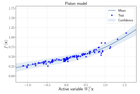
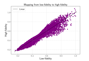
Figure 1: Left: sufficient summary plot of the surrogate model built with active subspaces. Right: correlation among the low-fidelity level and the high-fidelity level of the multi-fidelity model.

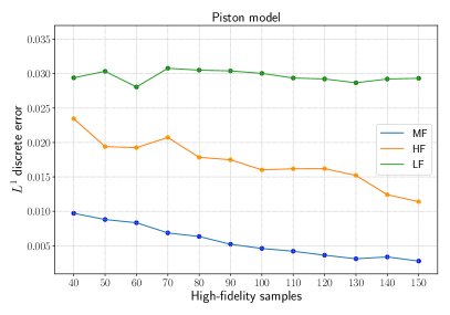
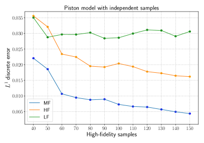
Figure 2: $L^{1}$ discrete error of the posterior of the multi-fidelity (MF), high-fidelity (HF) and low-fidelity (LF) models against the number of high-fidelity samples used to find the active subspace and build the Gaussian process regressions of the MF, HF, LF models. The 10000 test samples are distributed with Latin-Hypercube sampling. Left: identical high-fidelity samples for AS and NARGP. Right: independent high-fidelity samples for AS and NARGP.

It is qualitatively evident from the sufficient summary plot in the left panel of Figure 1 that a one-dimensional active subspace is enough to explain with a fairy good accuracy the dependence of the output from the $7$-dimensional inputs. This statement could be supported looking at the ordered eigenvalues of the correlation matrix of the gradients, which would show a spectral gap between the first and the second eigenvalues. We can also see in the right panel of Figure 1 the correlations scatter plot among the two different fidelity levels of the NARGP model. The low-fidelity GP regression built on the dataset $\{(x^{L}_{i},y^{L}_{i})\}_{i=1}^{N_{L}}$ performs already a good regression without many outliers in the predictions evaluated at the test samples.

Figure 2 shows the errors of the MF models built with different procedures, as described in Section 4. It can be seen that using independent samples for the active subspace evaluation does not improve the predictions obtained. Since in the right panel one third of the high-fidelity samples are used to identify the active subspace, to evaluate the differences between the two algorithms we have to compare the $150$ samples on the right with the $100$ samples on the left, for example. We can clearly notice that the two approches perform almost the same.

SEIR model for Ebola

The SEIR model for the spread of Ebola depends on $8$ parameters and the output of interest is the basic reproduction number $R_{0}$. A complete AS analysis was made in [10], while a kernel-based active subspaces comparison can be found in [30]. The formulation is the following:

$$R_{0}=\frac{\beta_{1}+\frac{\beta_{2}\rho_{1}\gamma_{1}}{\omega}+\frac{\beta_{3}}{\gamma_{2}}\psi}{\gamma_{1}+\psi},$$ (15)

where the parameters range are taken from [10].

Differently from the previous test case, the one-dimensional response function in the left panel of Figure 3 does not explain well the model: in this case kernel-based active subspaces could be employed to reach a better expressiveness of the surrogate model [30]. Even the scatter plot in the right panel of Figure 3, which shows the correlations between the low-fidelity and high-fidelity levels of the NARGP model, exhibits a worse accuracy in the low-fidelity level with respect to the previous test case. These results are quantified in Figure 4 with the $L^{1}$ discrete error for the different fidelities models which are one order of magnitude higher than the piston model, see Figure 2.

From a comparison between the HF and MF models in Figure 4 and the respective models in Figure 2 it can be seen that the nonlinear autoregressive fidelity fusion approach learns relatively worse correlations of the low-/high-fidelity levels of the NARGP Ebola model with respect to the piston model.

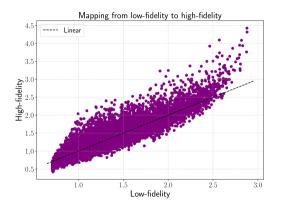
Figure 3: Left: sufficient summary plot of the Ebola model, 150 samples were used to build the AS surrogate model shown. Right: correlation among the low-fidelity level and the high-fidelity level of the multi-fidelity model.

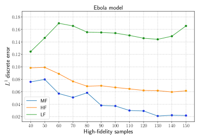
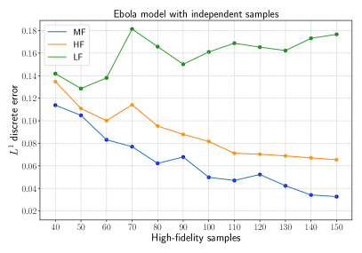
Figure 4: $L^{1}$ discrete error of the posterior of the multi-fidelity (MF), high-fidelity (HF) and low-fidelity (LF) models against the number of high-fidelity samples used to find the active subspace and build the Gaussian process regressions of the MF, HF, LF models. The 10000 test samples are distributed with Latin-Hypercube sampling. Left: identical high-fidelity samples for AS and NARGP. Right: independent high-fidelity samples for AS and NARGP.

For both the test cases the multi-fidelity regression approach with active subspaces results in better performance with a consistent reduction of the $L^{1}$ discrete error over a test dataset of $10000$ points.

6 Conclusions

In this work we propose a nonlinear multi-fidelity approach for the approximation of scalar function with low intrinsic dimensionality. Such dimension is identified by searching for the existence of an active subspace for the function of interest. With a regression along the active variable we build a low-fidelity model over the full parameter space which is fast to evaluate and does not need any new simulations. We just extract new information from the high-fidelity data we already have. This multi-fidelity approach results in a decreased regression error and improved approximation capabilities over all the parameter space.

We apply the multi-fidelity with AS method to two different benchmark problems involving high dimensional scalar functions with an active subspace. We achieve promising results with a reduction of the $L^{1}$ discrete error around $60$–$70\%$ with respect to the high-fidelity regression in one case (piston) and around $20$–$66\%$ in the other one (Ebola), depending on the number of high-fidelity samples used.

Further investigation will involve the use of more active subspaces based fidelities, such as the kernel active subspaces [30]. This could also greatly improve data-driven non-intrusive reduced order methods [32, 33, 34, 38] through modal coefficients reconstruction and prediction for parametric problems. We also mention the possible application to shape optimization problems for the evaluation of both the target function and the constraints.

References

- [1] E. N. Ben-Ari and D. M. Steinberg. Modeling data from computer experiments: an empirical comparison of kriging with MARS and projection pursuit regression. Quality Engineering, 19(4):327–338, 2007.
- [2] L. Bonfiglio, P. Perdikaris, S. Brizzolara, and G. Karniadakis. Multi-fidelity optimization of super-cavitating hydrofoils. Computer Methods in Applied Mechanics and Engineering, 332:63–85, 2018.
- [3] L. Bonfiglio, P. Perdikaris, G. Vernengo, J. S. de Medeiros, and G. Karniadakis. Improving swath seakeeping performance using multi-fidelity Gaussian process and Bayesian optimization. Journal of Ship Research, 62(4):223–240, 2018.
- [4] P. G. Constantine. Active subspaces: Emerging ideas for dimension reduction in parameter studies. SIAM, 2015.
- [5] P. G. Constantine and P. Diaz. Global sensitivity metrics from active subspaces. Reliability Engineering & System Safety, 162:1–13, 2017.
- [6] A. Damianou and N. Lawrence. Deep Gaussian processes. In Artificial Intelligence and Statistics, pages 207–215, 2013.
- [7] N. Demo, M. Tezzele, A. Mola, and G. Rozza. An efficient shape parametrisation by free-form deformation enhanced by active subspace for hull hydrodynamic ship design problems in open source environment. In Proceedings of ISOPE 2018: The 28th International Ocean and Polar Engineering Conference, pages 565–572, 2018.
- [8] N. Demo, M. Tezzele, and G. Rozza. A non-intrusive approach for reconstruction of POD modal coefficients through active subspaces. Comptes Rendus Mécanique de l’Académie des Sciences, DataBEST 2019 Special Issue, 347(11):873–881, November 2019.
- [9] N. Demo, M. Tezzele, and G. Rozza. A supervised learning approach involving active subspaces for an efficient genetic algorithm in high-dimensional optimization problems. arXiv preprint arXiv:2006.07282, Submitted, 2020.
- [10] P. Diaz, P. Constantine, K. Kalmbach, E. Jones, and S. Pankavich. A modified seir model for the spread of ebola in western africa and metrics for resource allocation. Applied Mathematics and Computation, 324:141–155, 2018.
- [11] A. I. Forrester, A. Sóbester, and A. J. Keane. Multi-fidelity optimization via surrogate modelling. Proceedings of the Royal Society A: Mathematical, Physical and Engineering Sciences, 463(2088):3251–3269, 2007.
- [12] GPy. GPy: A gaussian process framework in python. http://github.com/SheffieldML/GPy, since 2012.
- [13] J. L. Jefferson, J. M. Gilbert, P. G. Constantine, and R. M. Maxwell. Active subspaces for sensitivity analysis and dimension reduction of an integrated hydrologic model. Computers & Geosciences, 83:127–138, 2015.
- [14] M. Kanagawa, P. Hennig, D. Sejdinovic, and B. K. Sriperumbudur. Gaussian processes and kernel methods: A review on connections and equivalences. arXiv preprint arXiv:1807.02582, 2018.
- [15] M. C. Kennedy and A. O’Hagan. Predicting the output from a complex computer code when fast approximations are available. Biometrika, 87(1):1–13, 2000.
- [16] B. Kramer, A. N. Marques, B. Peherstorfer, U. Villa, and K. Willcox. Multifidelity probability estimation via fusion of estimators. Journal of Computational Physics, 392:385–402, 2019.
- [17] R. R. Lam, O. Zahm, Y. M. Marzouk, and K. E. Willcox. Multifidelity dimension reduction via active subspaces. SIAM Journal on Scientific Computing, 42(2):A929–A956, 2020.
- [18] M. Lázaro-Gredilla, J. Quiñonero-Candela, C. E. Rasmussen, and A. R. Figueiras-Vidal. Sparse spectrum Gaussian process regression. The Journal of Machine Learning Research, 11:1865–1881, 2010.
- [19] M. Lázaro-Gredilla and M. K. Titsias. Variational heteroscedastic Gaussian process regression. In ICML, 2011.
- [20] L. Le Gratiet and J. Garnier. Recursive co-kriging model for design of computer experiments with multiple levels of fidelity. International Journal for Uncertainty Quantification, 4(5), 2014.
- [21] H. Liu, Y.-S. Ong, X. Shen, and J. Cai. When Gaussian process meets big data: A review of scalable GPs. IEEE Transactions on Neural Networks and Learning Systems, 2020.
- [22] T. W. Lukaczyk, P. Constantine, F. Palacios, and J. J. Alonso. Active subspaces for shape optimization. In 10th AIAA multidisciplinary design optimization conference, page 1171, 2014.
- [23] X. Meng and G. E. Karniadakis. A composite neural network that learns from multi-fidelity data: Application to function approximation and inverse pde problems. Journal of Computational Physics, 401:109020, 2020.
- [24] A. Mola, M. Tezzele, M. Gadalla, F. Valdenazzi, D. Grassi, R. Padovan, and G. Rozza. Efficient reduction in shape parameter space dimension for ship propeller blade design. In R. Bensow and J. Ringsberg, editors, Proceedings of MARINE 2019: VIII International Conference on Computational Methods in Marine Engineering, pages 201–212, 2019.
- [25] A. Paleyes, M. Pullin, M. Mahsereci, N. Lawrence, and J. González. Emulation of physical processes with Emukit. In Second Workshop on Machine Learning and the Physical Sciences, NeurIPS, 2019.
- [26] P. Perdikaris, M. Raissi, A. Damianou, N. D. Lawrence, and G. E. Karniadakis. Nonlinear information fusion algorithms for data-efficient multi-fidelity modelling. Proceedings of the Royal Society A: Mathematical, Physical and Engineering Sciences, 473(2198):20160751, 2017.
- [27] J. Quinonero-Candela, C. E. Rasmussen, and C. K. Williams. Approximation methods for Gaussian process regression. In Large-scale kernel machines, pages 203–223. MIT Press, 2007.
- [28] M. Raissi, P. Perdikaris, and G. E. Karniadakis. Inferring solutions of differential equations using noisy multi-fidelity data. Journal of Computational Physics, 335:736–746, 2017.
- [29] M. Raissi, P. Perdikaris, and G. E. Karniadakis. Physics-informed neural networks: A deep learning framework for solving forward and inverse problems involving nonlinear partial differential equations. Journal of Computational Physics, 378:686–707, 2019.
- [30] F. Romor, M. Tezzele, A. Lario, and G. Rozza. Kernel-based Active Subspaces with application to CFD parametric problems using Discontinuous Galerkin method. arXiv preprint arXiv:2008.12083, Submitted, 2020.
- [31] F. Romor, M. Tezzele, and G. Rozza. ATHENA: Advanced Techniques for High dimensional parameter spaces to Enhance Numerical Analysis. Submitted, 2020.
- [32] G. Rozza, M. W. Hess, G. Stabile, M. Tezzele, and F. Ballarin. Basic Ideas and Tools for Projection-Based Model Reduction of Parametric Partial Differential Equations. In P. Benner, S. Grivet-Talocia, A. Quarteroni, G. Rozza, W. H. A. Schilders, and L. M. Silveira, editors, Handbook on Model Order Reduction, Vol. 2, chapter 1. De Gruyter, In Press, 2020.
- [33] G. Rozza, M. H. Malik, N. Demo, M. Tezzele, M. Girfoglio, G. Stabile, and A. Mola. Advances in Reduced Order Methods for Parametric Industrial Problems in Computational Fluid Dynamics. In R. Owen, R. de Borst, J. Reese, and P. Chris, editors, ECCOMAS ECFD 7 - Proceedings of 6th European Conference on Computational Mechanics (ECCM 6) and 7th European Conference on Computational Fluid Dynamics (ECFD 7), pages 59–76, Glasgow, UK, 2018.
- [34] F. Salmoiraghi, F. Ballarin, G. Corsi, A. Mola, M. Tezzele, and G. Rozza. Advances in geometrical parametrization and reduced order models and methods for computational fluid dynamics problems in applied sciences and engineering: Overview and perspectives. ECCOMAS Congress 2016 - Proceedings of the 7th European Congress on Computational Methods in Applied Sciences and Engineering, 1:1013–1031, 2016.
- [35] E. Snelson, Z. Ghahramani, and C. E. Rasmussen. Warped Gaussian processes. In Advances in neural information processing systems, pages 337–344, 2004.
- [36] M. Tezzele, F. Ballarin, and G. Rozza. Combined parameter and model reduction of cardiovascular problems by means of active subspaces and POD-Galerkin methods. In D. Boffi, L. F. Pavarino, G. Rozza, S. Scacchi, and C. Vergara, editors, Mathematical and Numerical Modeling of the Cardiovascular System and Applications, volume 16 of SEMA-SIMAI Series, pages 185–207. Springer International Publishing, 2018.
- [37] M. Tezzele, N. Demo, M. Gadalla, A. Mola, and G. Rozza. Model order reduction by means of active subspaces and dynamic mode decomposition for parametric hull shape design hydrodynamics. In Technology and Science for the Ships of the Future: Proceedings of NAV 2018: 19th International Conference on Ship & Maritime Research, pages 569–576. IOS Press, 2018.
- [38] M. Tezzele, N. Demo, A. Mola, and G. Rozza. An integrated data-driven computational pipeline with model order reduction for industrial and applied mathematics. Special Volume ECMI, In Press, 2020.
- [39] M. Tezzele, N. Demo, and G. Rozza. Shape optimization through proper orthogonal decomposition with interpolation and dynamic mode decomposition enhanced by active subspaces. In R. Bensow and J. Ringsberg, editors, Proceedings of MARINE 2019: VIII International Conference on Computational Methods in Marine Engineering, pages 122–133, 2019.
- [40] M. Tezzele, N. Demo, G. Stabile, A. Mola, and G. Rozza. Enhancing CFD predictions in shape design problems by model and parameter space reduction. Advanced Modeling and Simulation in Engineering Sciences, 7(40), 2020.
- [41] M. Tezzele, F. Salmoiraghi, A. Mola, and G. Rozza. Dimension reduction in heterogeneous parametric spaces with application to naval engineering shape design problems. Advanced Modeling and Simulation in Engineering Sciences, 5(1):25, Sep 2018.
- [42] C. K. Williams and C. E. Rasmussen. Gaussian processes for machine learning. MIT press Cambridge, MA, 2006.
- [43] O. Zahm, P. G. Constantine, C. Prieur, and Y. M. Marzouk. Gradient-based dimension reduction of multivariate vector-valued functions. SIAM Journal on Scientific Computing, 42(1):A534–A558, 2020.