Learning Monocular Dense Depth from Events

Abstract

Event cameras are novel sensors that output brightness changes in the form of a stream of asynchronous ”events” instead of intensity frames. Compared to conventional image sensors, they offer significant advantages: high temporal resolution, high dynamic range, no motion blur, and much lower bandwidth. Recently, learning-based approaches have been applied to event-based data, thus unlocking their potential and making significant progress in a variety of tasks, such as monocular depth prediction. Most existing approaches use standard feed-forward architectures to generate network predictions, which do not leverage the temporal consistency presents in the event stream. We propose a recurrent architecture to solve this task and show significant improvement over standard feed-forward methods. In particular, our method generates dense depth predictions using a monocular setup, which has not been shown previously. We pretrain our model using a new dataset containing events and depth maps recorded in the CARLA simulator. We test our method on the Multi Vehicle Stereo Event Camera Dataset (MVSEC). Quantitative experiments show up to 50% improvement in average depth error with respect to previous event-based methods.

Code and dataset are available at:
http://rpg.ifi.uzh.ch/e2depth

1 Introduction

Event cameras, such as the Dynamic Vision Sensor (DVS) [Lichtsteiner08ssc] or the ATIS [Posch10isscc], are bio-inspired vision sensors with radically different working principles compared to conventional cameras. While standard cameras capture intensity images at a fixed rate, event cameras only report changes of intensity at the pixel level and do this asynchronously at the time they occur. The resulting stream of events encodes the time, location, and sign of the change in brightness. Event cameras possess outstanding properties when compared to standard cameras. They have a very high dynamic range (140 dB versus 60 dB), no motion blur, and high temporal resolution (in the order of microseconds). Event cameras are thus sensors that can provide high-quality visual information even in challenging high-speed scenarios and high dynamic range environments, enabling new application domains for vision-based algorithms. Recently, these sensors have received great interest in various computer vision fields, ranging from computational photography [Rebecq19pami, Rebecq19cvpr, Scheerlinck18accv, Scheerlinck20wacv] to visual odometry [Rosinol18ral, Rebecq17ral, Rebecq17bmvc, Zhu17cvpr, Zhu19cvpr, Kim14bmvc] and depth prediction [Kim16eccv, Rebecq17ral, Rebecq16bmvc, Zhou18eccv, Zhu18eccv, Tulyakov19iccv, Zhu19cvpr]. The survey in [Gallego20pami] gives a good overview of the applications for event cameras.

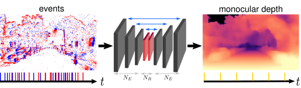
Figure 1: Method overview, the network receives asynchronous events inputs and predicts normalized log depth $\mathcal{\hat{D}}_{k}$. Our method uses $N_{R}$ recurrent blocks to leverage the temporal consistency in the events input.

Monocular depth prediction has focused primarily on on standard cameras, which work synchronously, i.e., at a fixed frame rate. State-of-the-art approaches are usually trained and evaluated in common datasets such as KITTI [Geiger13ijrr], Make3D [Saxena09pami] and NYUv2 [Silberman12eccv].

Depth prediction using event cameras has experienced a surge in popularity in recent years [Rosinol18ral, Rebecq16bmvc, Zhou18eccv, Rebecq17ral, Rebecq17bmvc, Kim16eccv, Zhu19cvpr, Zhou18eccv, Zhu18eccv, Tulyakov19iccv], due to its potential in robotics and the automotive industry. Event-based depth prediction is the task of predicting the depth of the scene at each pixel in the image plane, and is important for a wide range of applications, such as robotic grasping [Lenz15ijrr] and autonomous driving, with low-latency obstacle avoidance and high-speed path planning.

Method	Density	Monocular	Metric	Learning
			depth	based
[Rebecq17bmvc]	sparse	yes	yes	no
[Zhu17cvpr]	sparse	yes	yes	no
[Kim16eccv]	semi-dense	yes	no	no
[Rebecq17ral]	semi-dense	yes	yes	no
[Zhou18eccv]	semi-dense	no	yes	no
[Zhu18eccv]	semi-dense	no	yes	no
[Zhu19cvpr]	semi-dense	yes	yes	yes
[Tulyakov19iccv]	dense	no	yes	yes
Ours	dense	yes	yes	yes

Table 1: A literature review on event-based depth: model-based methods are listed top, learning-based methods are listed bottom. The type of output density is denoted with ”sparse” (depth at pixels when only events occurred), ”semi-dense” (depth at the reconstructed edges on the image), and ”dense” (depth prediction at all pixels). Note than only [Tulyakov19iccv] addresses dense per-pixel depth, but their work uses a stereo setup.

However, while event-cameras have appealing properties they also present unique challenges. Due to the working principles of the event camera, they respond predominantly to edges in the scene, making event-based data inherently sparse and asynchronous. This makes dense depth estimation with an event camera challenging, especially in low contrast regions, which do not trigger events and, thus, need to be filled in. Prior work in event-based depth estimation has made significant progress in this direction, especially since the advent of deep learning. However, most existing works are limited: they can reliably only predict sparse or semi-dense depth maps [Rosinol18ral, Rebecq16bmvc, Zhou18eccv, Rebecq17ral, Rebecq17bmvc, Kim16eccv, Zhu19cvpr, Zhou18eccv, Zhu18eccv] or rely on a stereo setup to generate dense depth predictions [Tulyakov19iccv].

In this work, we focus on dense, monocular, and metric depth estimation using an event camera, which addresses the aforementioned limitations. To the best of our knowledge, this is the first time that dense monocular depth is predicted using only events (see Fig. 1). We show that our approach reliably generates dense depth maps overcoming the sparsity in a stream of events. Our methodology is based on learning methods and gives reliable results, setting a baseline for dense depth estimation using events. We release DENSE, a dataset recorded in CARLA, which comprises events, intensity frames, semantic labels, and depth maps. Our contributions are the following:

• A recurrent network that predicts dense per-pixel depth from a monocular event camera.

• The implementation of an event camera plugin in the CARLA [Dosovitskiy17corl] simulator.

• DENSE - Depth Estimation oN Synthetic Events: a new dataset with synthetic events and perfect ground truth.

• Evaluation of our method on the popular Multi-Vehicle Stereo Event-Camera (MVSEC) Dataset [Zhu18ral] where we show improved performance with respect to the state of the art.

2 Related Work

2.1 Classical Monocular Depth Estimation

Early work on depth prediction used probabilistic methods and feature-based approaches. The K-means clustering approach was used by Achanta et al [Acharta12pami] to generate superpixel methods to improve segmentation and depth. Another work proposed multi-scale features with Markov Random Field (MRF) [Saxena06nips]. These methods tend to suffer in uncontrolled settings, especially when the horizontal alignment condition does not hold.

Deep Learning significantly improved the estimate driven by convolutional neural networks (CNN) with a variety of methods. The standard approach is to collect RGB images with ground truth labels and train a network to predict depth on a logarithmic scale. The network is trained in standard datasets that are captured with a depth sensor such as laser scanning. Eigen et al [eigen2015predicting] presented the first work training a multi-scale CNN to estimate depth in a supervised fashion. More specifically, the architecture consists of two parts, a first estimation based on Alexnet and a second refinement prediction. Their work led to successively major advances in depth prediction [Godard17cvpr, godard2019digging, wang2018learning, Li18cvpr, fu2018deep]. Better losses such as ordinal regression, multi-scale gradient, and reverse Huber (Berhu) loss were proposed in those works. Another set of approaches is to jointly estimate poses and depth in a self-supervised manner. This is the case of Zhou et al [zhou2017unsupervised]. Their work proposes to simultaneously predict both pose and depth with an alignment loss computed from the warped consecutive images. Most of the previous works, except for of [Li18cvpr], are specific for the scenario where they have been trained and, thus, they are not domain independent.

2.2 Event-based Depth Estimation

Early works on event-based depth estimation used multi-view stereo [Rebecq16bmvc] and later Simultaneous Localization and Mapping (SLAM) [Rebecq17ral, Rosinol18ral, Zhu17cvpr, Kim16eccv] to build a representation of the environment (i.e.: map) and therefore derivate metric depth. These approaches are model-based methods that jointly calculate pose and map by solving a non-linear optimization problem. Model-based methods can be divided into feature-based methods that produce sparse point clouds and direct methods that generate semi-dense depth maps. Both methods either use the scale given by available camera poses or rely on auxiliary sensors such as inertial measurement units (IMU) to recover metric depth.

Purely vision-based methods have investigated the use of stereo event cameras for depth estimation [Zhou18eccv, Zhu18eccv] in which they rely on maximizing a temporal (as opposed to photometric) consistency between the pair of event camera streams to perform disparity and depth estimation. Recently, several learning-based approaches have emerged that have led to significant improvements in depth estimation [Zhu19cvpr, Tulyakov19iccv]. These methods have demonstrated more robust performance since they can integrate several cues from the event stream. Among these, [Zhu19cvpr] presents a feed-forward neural network that jointly predicts relative camera pose and per-pixel disparities. Training is performed using stereo event camera data, similar to [Godard17cvpr], and testing is done using a single input. However, this method still generates semi-dense depth maps, since a mask is applied to generate event frame depths at pixels where an event occurred. The work in [Tulyakov19iccv] overcomes these limitations by fusing data from stereo setup to produce dense metric depth but still relies on a stereo setup and a standard feed-forward architecture. Our work compares to the learning-based approaches but goes one step further by predicting dense metric depth for a single monocular camera. We achieve this by exploiting the temporal consistency of the event stream with a recurrent convolution network architecture and training on synthetic and real data. Table 1 provides a comparison of among state of the art methods, model-based and learning-based, where our proposed approach exceeds by grouping all the listed features.

3 Depth Estimation Approach

Events cameras output events at independent pixels and do this asynchronously. Specifically, their pixels respond to changes in the spatio-temporal log irradiance $L(\mathbf{u},t)$ that produces a stream of asynchronous events. For an ideal sensor, an event $e_{i}=(\mathbf{u}_{i},t_{i},p_{i})$ is triggered at time $t_{i}$ if the brightness change at the pixel $\mathbf{u}_{i}=(x_{i},y_{i})^{\intercal}$ exceeds a threshold of $\pm C$. The event polarity $p_{i}$ denotes the sign of this change.

Our goal is to predict dense monocular depth from a continuous stream of events. The method works by processing subsequent non-overlapping windows of events $\epsilon_{k}=\{e_{i}\}_{i=0}^{N-1}$ each spanning a fixed interval $\Delta T=t^{k}_{N-1}-t^{k}_{0}$. For each window, we predict log depth maps $\{\mathcal{\hat{D}}_{k}\}$, with $\mathcal{\hat{D}}_{k}\in[0,1]^{W\times H}$. We implement log depth prediction as a recurrent convolutional neural network with an internal state $\mathbf{s}_{k}$. We train our network in a supervised manner, using ground truth depth maps. The network is first trained in simulation using perfect ground truth and synthetic events and finetuned in a real sequence.

3.1 Event Representation

Due to the sparse and asynchronous nature of event data, batches of events $\epsilon_{k}$ need to be converted to tensor-like representations $\textbf{E}_{k}$. One way to encode these events is by representing them as a spatio-temporal voxel grid [Zhu19cvpr, Gehrig19iccv] with dimensions $B\times H\times W$. Events within the time window $\Delta T$ are collected into $B$ temporal bins according to

$$\textbf{E}_{k}(\mathbf{u}_{k},t_{n})=\sum_{e_{i}}p_{i}\delta(\mathbf{u}_{i}-\mathbf{u}_{k})\max(0,1-|t_{n}-t^{*}_{i}|)$$ (1)

where $t_{i}^{*}=\frac{B-1}{\Delta T}(t_{i}-t_{0})$ is the normalized event timestamp. In our experiments, we used $\Delta T=50ms$ of events and $B=5$ temporal bins. To facilitate learning, we further normalize the non-zero values in the voxel grid to have zero mean and unit variance.

3.2 Network Architecture

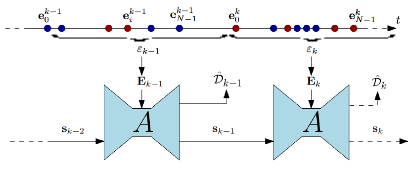
Figure 2: Our network architecture, image adapted from [Rebecq19pami]. The event stream is grouped into non-overlapping windows of events and converted to tensor-like voxel grids [Zhu19cvpr]. These voxel grids are passed to our recurrent fully convolutional neural network to produce normalized log depth predictions.

It consists of a recurrent, fully convolutional neural network, based on the UNet architecture [Ronneberger15icmicci]. The network input is first processed by a head layer $\mathcal{H}$ and then $N_{E}$ recurrent encoder layers ($\mathcal{E}^{i})$ followed by $N_{R}$ residual blocks ($\mathcal{R}^{j}$) and $N_{E}$ decoder layers $\mathcal{D}^{l}$. A final depth prediction layer $\mathcal{P}$ produces the output of our network. The head layer produces an output with $N_{b}$ channels, which is doubled at each encoder layer, resulting in a feature map with $N_{b}\times 2^{N_{E}}$ output channels. $\mathcal{P}$ performs a depth-wise convolution with one output channel and kernel size 1. We use skip connections between symmetric encoder and decoder layers (see Fig. 2). At the final layer, the activations are squashed by a sigmoid activation function. Each encoder layer is composed of a downsampling convolution with kernel size 5 and stride 2 and a ConvLSTM [Shi15nips] module with kernel size 3. The encoding layers maintain a state $c_{k}^{i}$ which is at 0 for $k=0$. The residual blocks use a kernel size of 3 and apply summation over the skip connection. Finally, each decoder layer is composed of a bilinear upsampling operation followed by convolution with kernel size 5. We use ReLU except for the prediction layer, and batch normalization [Ioffe15icml]. In this work we use $N_{E}=3$, $N_{R}=2$ and $N_{b}=32$ and we unroll the network for $L=40$ steps.

3.3 Depth Map Post-processing

As usual, in recent work on depth prediction, we train our network to predict a normalized log depth map. Log depth maps have the advantage of representing large depth variations in a compact range, facilitating learning. If $\mathcal{\hat{D}}_{k}$ is the depth predicted by our model, the metric depth can be recovered by performing the following operations:

$$\mathcal{\hat{D}}_{m,k}=\mathcal{D}_{\text{max}}\exp(-\alpha(1-\mathcal{\hat{D}}_{k}))$$ (2)

Where $\mathcal{D}_{\text{max}}$ is the maximum expected depth and $\alpha$ is a parameter chosen, such that a depth value of 0 maps to minimum observed depth. In our case, $\mathcal{D}_{\text{max}}=80$ meters and $\alpha=3.7$ corresponding to a minimum depth of $~{}2$ meters.

3.4 Training Details

We train our network in a supervised fashion, by minimizing the scale-invariant and multi-scale scale-invariant gradient matching losses at each time step. Given a sequence of ground truth depth maps $\{\mathcal{D}_{k}\}$, denote the residual $\mathcal{R}_{k}=\mathcal{\hat{D}}_{k}-\mathcal{D}_{k}$. Then the scale-invariant loss is defined as

$$\mathcal{L}_{k,\text{si}}=\frac{1}{n}\sum_{\textbf{u}}(\mathcal{R}_{k}(\textbf{u}))^{2}-\frac{1}{n^{2}}\left(\sum_{\textbf{u}}\mathcal{R}_{k}(\textbf{u})\right)^{2},$$ (3)

where $n$ is the number of valid ground truth pixels u. The multi-scale scale-invariant gradient matching loss encourages smooth depth changes and enforces sharp depth discontinuities in the depth map prediction. It is computed as follows:

$$\mathcal{L}_{k,\text{grad}}=\frac{1}{n}\sum_{s}\sum_{\textbf{u}}|\nabla_{x}\mathcal{R}^{s}_{k}(\textbf{u})|+|\nabla_{y}\mathcal{R}^{s}_{k}(\textbf{u})|.$$ (4)

Here $\mathcal{R}^{s}_{k}(\textbf{x})$ refers to the residual at scale $s$ and the $L_{1}$ norm is used to enforce sharp depth discontinuities in the prediction. In this work, we consider four scales, similar to [Li18cvpr]. The resulting loss for a sequence of $L$ depth maps is thus

$$\mathcal{L}_{\text{tot}}=\sum_{k=0}^{L-1}\mathcal{L}_{k,\text{si}}+\lambda\mathcal{L}_{k,\text{grad}}.$$ (5)

The hyper-parameter $\lambda=0.5$ was chosen by cross-validation. We train with a batch size of 20 and a learning rate of $10^{-4}$ and use the Adam [Kingma15iclr] optimizer.

Our network requires training data in the form of events sequences with corresponding depth maps. However, it is difficult to get perfect dense ground truth depth maps in real datasets. For this reason, we propose to first train the network using synthetic data and get the final metric scale by finetuning the network using real events from the MVSEC dataset.

We implement an event camera sensor in CARLA [Dosovitskiy17corl] based on the previous event simulator ESIM [Rebecq18corl]. The event camera sensor takes the rendered images from the simulator environment and computes per-pixel brightness change to simulate an event camera. The computation is done at a configurable but fixed high framerate (we use $20$ times higher than the images frame rate) to approximate the continuous signal of a real event camera. The simulator allows us to capture a variety of scenes with different weather conditions and illumination properties. The camera parameters are set to mimic the event camera at MVSEC with a sensor size of $346\times 260$ pixels (resolution of the DAVIS346B) and a focal length of $83^{\circ}$ horizontal field of view.

We split DENSE, our new dataset with synthetic events, into five sequences for training, two sequences for validation, and one sequence for testing (a total of eight sequences). Each sequence consists of 1000 samples at $30$ FPS (corresponding to $33$ seconds), each sample is a tuple of one RGB image, the stream of events between two consecutive images, ground truth depth, and segmentation labels. Note that only the events and the depth, maps are used by the network for training. RGB images are provided for visualization and segmentation labels complete the dataset with richer information. CARLA Towns 01 to 05 are the scenes for training, Town 06 and 07 for validation, and the test sequence is acquired using Town 10. This split results in an overall of $5000$ samples for training, $2000$ samples for validation, and $1000$ samples for testing.

4 Experiments

In this section, we present qualitative and quantitative results and compare them with previous methods [Zhu19cvpr] on the MVSEC dataset. We focus our evaluation on real event data while the evaluation on synthetic data is detailed in Appendix A.

Training set	Dataset	Abs Rel$\downarrow$	Sq Rel $\downarrow$	RMSE$\downarrow$	RMSE log$\downarrow$	SI log$\downarrow$	$\bm{\delta<1.25\uparrow}$	$\bm{\delta<1.25^{2}\uparrow}$	$\bm{\delta<1.25^{3}\uparrow}$
S		0.698	3.602	12.677	0.568	0.277	0.493	0.708	0.808
R	outdoor day1	0.450	0.627	9.321	0.514	0.251	0.472	0.711	0.823
S* $\rightarrow$ R		0.381	0.464	9.621	0.473	0.190	0.392	0.719	0.844
S* $\rightarrow$ (S+R)		0.346	0.516	8.564	0.421	0.172	0.567	0.772	0.876
S		1.933	24.64	19.93	0.912	0.429	0.293	0.472	0.600
R	outdoor night1	0.770	3.133	10.548	0.638	0.346	0.327	0.582	0.732
S* $\rightarrow$ R		0.554	1.798	10.738	0.622	0.343	0.390	0.598	0.737
S* $\rightarrow$ (S+R)		0.591	2.121	11.210	0.646	0.374	0.408	0.615	0.754
S		0.739	3.190	13.361	0.630	0.301	0.361	0.587	0.737
R	outdoor night2	0.400	0.554	8.106	0.448	0.176	0.411	0.720	0.866
S* $\rightarrow$ R		0.367	0.369	9.870	0.621	0.279	0.422	0.627	0.745
S* $\rightarrow$ (S+R)		0.325	0.452	9.155	0.515	0.240	0.510	0.723	0.840
S		0.683	1.956	13.536	0.623	0.299	0.381	0.593	0.736
R	outdoor night3	0.343	0.291	7.668	0.410	0.157	0.451	0.753	0.890
S* $\rightarrow$ R		0.339	0.230	9.537	0.606	0.258	0.429	0.644	0.760
S* $\rightarrow$ (S+R)		0.277	0.226	8.056	0.424	0.162	0.541	0.761	0.890

Table 2: Ablation study and evaluation of MVSEC. All rows are the same network with the change in the training set. The Training set is denoted with $S$ (synthetic data from the DENSE training split), $R$ (real data from the training split in outdoor day2 sequence), $S^{*}$ (first 1000 samples of the DENSE training split), $S^{*}\rightarrow R$ (pretrained on $S^{*}$ and retrained on $R$), $S^{*}\rightarrow(S+R)$ (pretrained on $S^{*}$ and retrained on both datasets). $\downarrow$ indicates lower is better and $\uparrow$ higher is better. The results are the driving sequences of MVSEC (except for outdoor day2). Best values are shown in bold.

$\begin{array}{c}\end{array}$

(a) Events

(b) DepthtrainedonlyonSdata

(c) Depthtrainedonl