Lubricated gravity currents of power-law fluids

Abstract

The motion of glaciers over their bedrock or drops of fluid along a solid surface can vary dramatically when these substrates are lubricated. We investigate the coupled flow of a gravity current (GC) of strain-rate softening fluid that is lubricated by a denser, lower-viscosity Newtonian fluid. We present a set of experiments in which such GCs are discharged axisymmetrically and at constant flux over a flat surface. Using imaging techniques we follow the front evolution of each fluid and their thickness field. We find that the two fronts of our lubricated GCs evolve faster than non-lubricated GCs, though with similar time exponents. In addition, the thickness of the non-Newtonian fluid is nearly uniform while that of the lubricating fluid is nonmonotonic with localised spikes. Nevertheless, lubricated GCs remain axisymmetric as long as the flux of the lubricating fluid is sufficiently smaller than the non-Newtonian fluid flux.

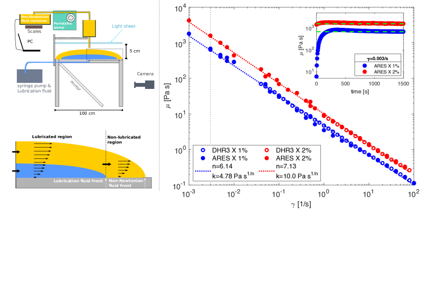
Figure 1: ($a$) Our experimental apparatus for lubricated GCs. ($b$) Close-up of the flow region (dash-line rectangular in $(a)$). (c) Viscosity measurements of Xanthan solutions as a function of strain rate ($\bullet$, $\circ$) and the regression to power-law function ($\bullet$$\bullet$$\bullet$$\bullet$). Inset shows the evolution of the viscosity measurement at strain rate 0.003/s.

I Introduction

Gravity-driven flows of one fluid over another can involve complex interactions between the two fluids, which can lead to a rich dynamical behavior. Such flows occur in a wide range of natural and human-made systems, as in lava flow over less viscous lava (Griffiths, 2000; Balmforth et al., 2000), spreading of the lithosphere over the mid-mantle boundary (Lister and Kerr, 1989; Dauck et al., 2019), ice flow over an ocean (DeConto and Pollard, 2016; Kivelson et al., 2000) and over bedrock covered with sediments and water (Stokes et al., 2007; Fowler, 1987), flows in porous media (Woods and Mason, 2000), and droplets motion on liquid-infused surfaces (Keiser et al., 2017).

The flow of GCs in circular geometry has been studied with a range of boundary conditions. At the absence of a lubricating layer, a common boundary condition along the base of the sole GC is no slip. Such GCs of Newtonian fluids that are discharged at constant flux follow a similarity solution, in which the front position at time $t$ is proportional to $t^{1/2}$ (Huppert, 1982). Similar GCs of power-law (PL) fluids having exponent $n$, where $n=1$ represents a Newtonian fluid and $n>1$ represents a strain-rate softening fluid, also have similarity solutions in which the front propagation is proportional to $t^{(2n+2)/(5n+3)}$ (Sayag and Worster, 2013).

On the other extreme, the presence of a lower fluid layer can significantly reduce friction at the base of the top fluid, resulting in extensionally dominated GCs. This is the case, for example, for ice shelves, which deform over the relatively inviscid oceans with weak friction along their interface. The late-time front evolution of such axisymmetric GCs of Newtonian fluids is proportional to $t$ (Pegler and Worster, 2012). However, when the top fluid is strain-rate softening, an initially axisymmetric front can destabilise and develop fingering patterns that consist of tongues separated by rifts (Sayag and Worster, 2019).

In the more general case the conditions along the boundaries of the GCs can vary spatiotemporally, as their stress field evolves. For example, the interface of an ice sheet with its underlying bed rock can include distributed melt water and sediments, which impose nonuniform and time-dependent friction along the ice base, and evolves spatiotemporally under the stresses imposed by the ice layer. Consequently, the coupled ice-lubricant system may evolve different flow patterns (Stokes et al., 2007; Fowler, 1987). Such systems were modelled as two coupled GC of Newtonian fluids spreading one on top of the other (Kowal and Worster, 2015). The early stage of these flows follows a self similar evolution, in which the fronts of the two fluids evolve like $t^{1/2}$, as in non-lubricated (no-slip) GCs, and they can have radially non-monotonic thickness. However, experiments showed that at a later stage these coupled flows became unstable and developed fingering patterns and non-axisymmetric flow (Kowal and Worster, 2015).

In this study we investigate a similar system as in Kowal and Worster (2015), only with a non-Newtonian (strain-rate softening) GC as the top layer. We explore experimentally the case where the flux and viscosity of the lubricating fluid is much smaller than the non-Newtonian fluid. We trace the evolution of the two front, and the spatiotemporal evolution of the light transmission through the two fluids, from which we resolve the thickness distribution of the top-layer, non-Newtonian fluid. We then contrast our findings with the present theories of non-lubricated and lubricated GCs.

II Experimental setup

The experimental apparatus (Figure 1a,b) included a flat, optically-transparent square glass sheet of 1x1 m² and 10 mm thickness, supported by an aluminum frame parallel to the ground with a 50 micron/m alignment accuracy. A rectangular plane mirror was placed underneath the glass sheet at an angle 45^∘ to the horizontal for imaging. The center of the glass sheet had a 5 mm diameter nozzle that was connected to a syringe pump (NE4000) that delivered the lubricating fluid. The non-Newtonian fluid was driven by gravity from a beaker that was supported by an xyz-translation stage through an 8 mm diameter aluminium tube, whose outlet was 15 mm over the glass surface (Figure 1a,b). We kept the flux constant by keeping a constant fluid level in the beaker using a peristaltic pump that supplied fluid from a reservoir. A 1x1 m² white light-sheet and a diffuser were positioned parallel to the glass surface and about 50 mm over it to illuminate the flow uniformly. Time-lapsed image sequence was captured throughout each experiment using Nikon D5500 camera that was facing the 45^∘ mirror.

Experiment	c	$Q$
Non-lubricated GC	%/w	g/s
GLSns1  $\bullet$	1	1.673
GLSns2  $\blacksquare$	1	1.669
GLSs $\bigstar$	2	0.909
GLSns3 $\blacktriangleleft$	2	0.917
ACRns1 ✶	2	0.812
ACRns2 $\bullet$	2	0.811

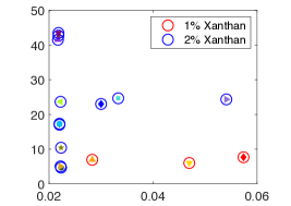
Experiment	$\mathscr{Q}$	$\mathscr{M}$	c	$Q$	$t_{L}$	$r_{N}(t_{L})$
Lubricated GC	-	-	%/w	g/s	s	cm
1  $\blacklozenge$	0.0574	7661	1	1.167	798	20
2  $\blacktriangle$	0.0283	6936	1	1.767	752	20
3 $\blacktriangledown$	0.04697	6006	1	1.767	594	20
4a $\bullet$	0.0223	4671	2	4.716	78	10
5  $\blacksquare$	0.0218	42717	2	0.643	1550	20
6  $\blacktriangleright$	0.0222	5023	2	3.643	82	10
7a $\blacktriangleleft$	0.0222	23639	2	1.5	754	20
8  $\bigstar$	0.0223	10412	2	1.525	208	10
9  ✶	0.022	17036	2	1.5	450	15
10 $\bullet$	0.022	17323	2	1.5	462	15
11 $\blacksquare$	0.0333	24661	2	1.5	806	20
12 $\blacklozenge$	0.03	23017	2	1.664	742	20
13a$\blacktriangle$	0.0217	41528	2	0.692	1510	20
14 $\blacktriangledown$	0.0218	43483	2	0.643	1594	20
15 $\blacktriangleright$	0.0541	24343	2	1.533	794	20

Figure 2: (Table a) The non-lubricated GC experiments were performed on Glass (GLS) or Acrylic (ACR) substrates with a pre-coat of soap solution (s) or without one (ns). (b) The lubricated GC experiments in the $\mathscr{M}-\mathscr{Q}$ state space. (Table c) The lubricated GC experiments. All experiments were performed at 22^∘C.

II.1 Preparation & Properties of the experimental fluids

The non-Newtonian fluid we used was an aqueous solution of food-grade Xanthan gum (Jungbunzlauer) of 1% and 2% concentration (per weight). To prepare a uniformly dissolved, and air-bubble-free solutions we followed the following procedure: First, we generated a smooth vortex (Eurostat-200) in a beaker containing deionized water. Then, we poured the Xanthan-gum powder into the center of the vortex within less than 60s, to ensure uniform dispersion of the powder and prevent aggregates before the viscosity of the solution soars. After 90 min of mixing we added 0.3 g of lemon-yellow color per 5000 g of solution, and stirred for additional 30 minutes. Finally, we stored the solution in a 4^∘C refrigerator for 24h to remove air bubbles. The densities of the solutions were 1.0035 and 1.007 gm/cm³ for the 1% and 2% concentrations, respectively.

The rheology of xanthan gum solutions of such concentrations has been studied extensively in various flow configurations, and we describe it in detail in Sayag and Worster (2019). In general, such xanthan solutions are viscoelastic. However, in flows such as the one we consider here the role of elastic deformation is significantly smaller compared with viscous deformation (e.g., Sayag and Worster, 2013, 2019). We support this by estimating the Deborah number for our flow in §IV. Therefore, here we focus on the viscous deformation of our xanthan solutions, which is known to be consistent with a PL fluid of both shear and extensional thinning for a wide range of strain rates, with an approximately similar exponent (Martín-Alfonso et al., 2018).

We used TA DHR-3 and ARES rheometers to measure the dependence of the shear viscosity $\mu$ of our xanthan solutions on the shear rate $\gamma$. The setup consisted of steady shear flow within a 2^∘-cone-and-plate geometry (40 mm (DHR-3), and 50 mm (ARES)) and a solvent trap to minimize dehydration. The rate of shear was varied monotonically in steps, and the measurement of the viscosity at each step continued until a steady value was reached (within $\pm 1\%$ STD). A weak-gel behaviour of the solution at low shear rates resulted in increasingly longer viscosity measurements with the decline in shear rate (Figure 1c, inset). Fitting our measured viscosity to the power-law relation

$$\mu=k\gamma^{{1/n}-1},$$

with the consistency $k$ and the exponent $n$ as free parameters, we find that $n=6.14,~{}7.14$ and $k=4.78,~{}10.05$ Pa s^1/n for the 1% and 2% solutions, respectively (Figure 1c).

For a lubricating fluid of larger density and lower viscosity, we used glucose solutions of density $\rho_{\ell}=1.164$ g/cm³ and dynamic viscosity of $\mu_{\ell}=9$ mPa s. We dyed the fluid in blue to get high contrast of the evolving fluid-fluid interface, and to measure the evolution of the non-Newtonian fluid thickness (§III)

II.2 Experimental procedure & preliminary experiments

Two preparation procedures had a major impact on the reproducibility of our experiments. The first was the accuracy of concentric alignment of the two outlet nozzles of the discharged fluids, which we did to an accuracy of $\pm 100$ $\mu$m using the xyz stage and an adapter that could fit simultaneously to both nozzles. The second procedure concerns the impact of the wetting conditions over the glass surface on the shape of the lubricating-fluid front. At the absence of the non-Newtonian fluid, the axisymmetry of that front was sensitive to the wetting conditions of the glass surface. We avoided this sensitivity by forming uniform wetting conditions over the glass surface using a coat of soap solution (3.3% liquid dish soap in deionized water) that was allowed to dehydrate prior to the initiation of our experiments. To verify that the soap coating had no impact on the non-Newtonian GC, we compared the front evolution of a non-lubricated GCs with and without a soap coating, and found no measurable difference for Xanthan concentrations of either 1% or 2% (Figure 2a).

We conducted 15 lubricated GC experiments (Figure 2c) in the following procedure. Initially, we released the non-Newtonian fluid axisymmetrically in constant flux. When the evolving GC reached a radius of 10-20 cm ($t=t_{L}$), we initiated the axisymmetric discharge of the lubricating fluid underneath the non-Newtonian fluid (Figure 3a, Movies 1-4).

III Experimental analysis

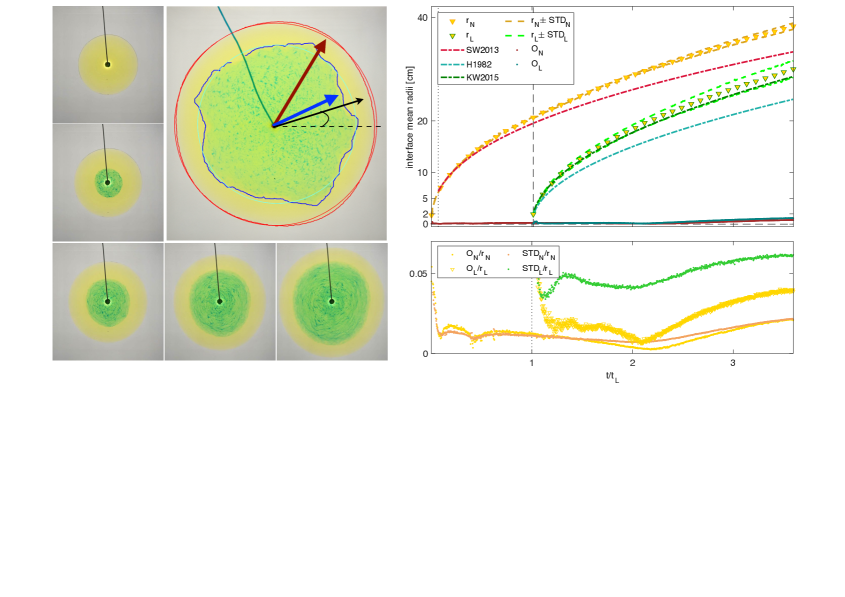
Figure 3: (a) Time series of snapshots from experiment #7, showing the Xanthan-solution (yellow) lubricated by a sugar solution (green). $(b)$ Snapshot from experiment #3 showing the resolved front of the lubricating (—) and the non-Newtonian fluids (—), and the fitted circles in (—) and (—), respectively. $(c)$ Evolution of the average front radii $r_{N},r_{L}$, centers $O_{N},O_{L}$, and STDs compared with theoretical predictions of lubricated and non-lubricated GCs. (d) STDs and centers $O_{N},O_{L}$ normalised by instantaneous $r_{N},r_{L}$.

We classify the lubricated GC experiments using the four dimensionless numbers

$$\displaystyle{\mathscr{Q}\equiv\frac{Q_{\ell}}{Q},} \displaystyle{\mathscr{D}\equiv\frac{\rho_{\ell}-\rho}{\rho},} n,$$

$$\mathscr{M}\equiv\frac{\mu}{\mu_{\ell}}= \,\displaystyle{\frac{\rho g}{\mu_{\ell}}\left(\frac{k}{\rho g}\right)^{\frac{8n}{5n+3}}\left(Qt_{L}^{-4}\right)^{\frac{1-n}{5n+3}},}$$ (1)

representing, respectively, the sources flux ratio, the reduced density ratio, the PL fluid exponent, and the viscosity ratio, in which we evaluate the scale of $\mu$ using the characteristic scales of a non-lubricated GC (Sayag and Worster, 2013). In the experiments we present, the lubrication flux was much smaller than the flux of the PL fluid ($\mathscr{Q}\lesssim 0.06$), the viscosity ratio varied over nearly one order of magnitude ($4700\lesssim\mathscr{M}\lesssim 43000$), and the 1% and 2% polymer concentrations led to a small variation of $n$ (Figure  1c) and to similar density ratios $\mathscr{D}_{2\%}=0.152$ and $\mathscr{D}_{1\%}=0.156$, respectively.

To explore the significance of the interaction between the two fluids, we analyse the image sequence of each experiment to trace the evolution of the two fluid fronts and fluid thicknesses, and we compare the resulted measurements to existing theories of lubricated and non-lubricated flows.

III.1 The front evolution of the lubricating and non-Newtonian fluids.

Tracing the position of the fronts of the non-Newtonian fluid $r_{N}(t,\theta)$ and of the lubricating fluid $r_{L}(t,\theta)$, where $\theta$ is the angular coordinate, we calculate the average radius of each instantaneous front by fitting a circle (Figure 3b). We find that the regression standard deviation (STD) can be reduced significantly when using the centers of the fitted circles $O_{N}$ and $O_{L}$ as additional free parameters (Figure 3c,d). This means that the deviation of the front from an axisymmetric shape has two contributions: the centers $O_{N},O_{L}$ that represent translation of the geometric center of the circular front, and the STD that represents the non-axisymmetric displacement of the front with respect to the translated circle. We find that STD${}_{L},O_{L}\lesssim 5$ cm, whereas STD${}_{N},O_{N}\lesssim 2$ cm, implying larger variations of the geometric center and non-axisymmetric component of the lubricating fluid compared with those of the non-Newtonian fluid. However, the ratio of the centers and STDs with the front radii remain confined and even decay (Figure 3d). Therefore, throughout the flow, the evolution of the fluid fronts remains axisymmetric to leading order.

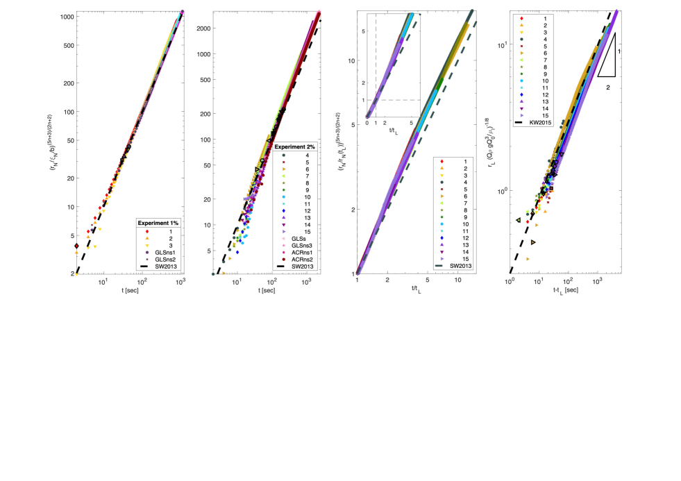
Figure 4: Evolution of the fluid fronts. (a, b) The front $r_{N}(t)$ during the non-lubricated interval ($t<t_{L}$), for the 1% (a) and 2% (b) concentrations. (c) The front $r_{N}(t)$ during the lubricated interval ($t>t_{L}$). Inset zooms to the earlier stage that includes the non-lubricated interval. The corresponding front $r_{N}^{SW13}$ of the non-lubricated GC (${\color[rgb]{.5,.5,.5}\hdashrule[0.5ex]{0.9cm}{1mm}{1.5mm}}$) has no fitting parameters (a,b,c). (d) The front $r_{L}(t)$ compared with $r_{L}^{KW15}$ (${\color[rgb]{0,0,0}\hdashrule[0.5ex]{0.9cm}{1mm}{1.5mm}}$). The markers when the thin-film criterion is first satisfied have black edges.

The resulted evolution of the fronts can be appreciated through contrasting with existing theories of non-lubricated GC of PL (Sayag and Worster, 2013) and Newtonian (Huppert, 1982) fluids, and lubricated GC of Newtonian fluids (Kowal and Worster, 2015), in which the solutions for the fronts are respectively

$$r_{N}^{\textrm{SW13}} =\xi_{N}b_{N}t^{{2n+2}\over{5n+3}}, b_{N} =\left[{{2^{1-n}}\over{n+2}}Q^{2n+1}\left({\rho g}\over{k}\right)^{n}\right]^{1/(5n+3)},$$ (2a)

$$r_{L}^{\textrm{H82}} =\xi_{L}b_{L}t^{1/2}, b_{L} =\left(Q_{\ell}^{3}({\rho_{\ell}-\rho})g\over{3\mu_{\ell}}\right)^{1/8},$$ (2b)

$$r_{L}^{\textrm{KW15}} =\xi_{L}^{*}b_{L}^{*}t^{1/2}, b_{L}^{*} =\left(\mathscr{MQ}Q^{3}{\rho g}\over{\mu}\right)^{1/8}=\left(\mathscr{Q}Q^{3}{\rho g}\over{\mu_{\ell}}\right)^{1/8},$$ (2c)

where for constant flux $\xi_{N}=\xi_{L}\approx 0.71$ and $\xi_{L}^{*}\approx 0.27\pm 0.02$. These similarity solutions are valid when the thin-film approximation is satisfied, i.e., when $r_{N}/h\gtrsim 10$, where $h$ is the characteristic thickness. We estimate this ratio by assuming that the instantaneous fluid volume $Qt$ is distributed as a disc of radius $r_{N}$ and thickness $h$. Therefore, the condition is $r_{N}/h=\pi r_{N}^{3}/Qt\gtrsim 10$ for the top fluid, and similarly, $r_{L}/h_{\ell}=\pi r_{L}^{3}/Q_{\ell}(t-t_{L})\gtrsim 10$ for the lubricating fluid.

We consider the evolution of the front $r_{N}$ of the non-Newtonian fluid separately during the non-lubricated interval ($t<t_{L}$, Figure 4a,b), and the lubricated interval (Figure 4c). In the first interval we expect the front to evolve consistently with (2a) as soon as the lubrication-approximation condition is satisfied. We find that our measurements for the 1% solutions indeed collapse to the theoretical predictions (Figure 4a). For the 2% solutions our measured front propagates faster than the theoretical prediction (Figure 4b). Our preliminary experiments (Figures 2a, 4a,b) indicate that this discrepancy is independent of the substrate wetting conditions or the substrate material (glass or acrylic). Therefore, we believe that wall slip may arise at high polymer concentrations, as we elaborate in §IV. In the lubricated interval ($t\geq t_{L}$), we measure faster propagation of $r_{N}$ than a non-lubricated GC (Figure 4c), which implies a significant impact of lubrication. The response of $r_{N}$ to the lubrication fluid initialises with a transient acceleration ($1.5\lesssim t/t_{L}\lesssim 5$) with respect to the non-lubricated solution, then ($5\lesssim t/t_{L}$) the front evolves with a similar exponent as the non-lubricated solution (eq. 2a), but faster.

The flow of the lubricating fluid is affected by both the normal and shear stresses applied by the surrounding non-Newtonian fluid. Nevertheless, we find that the evolution of $r_{L}$ is power law in time with an exponent 1/2 (Figure 4d), similar to the exponent predicted for Newtonian Ks (Huppert, 1982; Kowal and Worster, 2015). However, our measured intercept deviates from the theoretical prediction (Figure 4d), implying that it may have dependence on the properties of the non-Newtonian fluid, which is absent in the intercept $b_{L}^{*}$ of the Newtonian theory (2c). We also note that for all the experiments

$$b_{L}/b_{L}^{*}=\left(\tfrac{1}{3}\mathscr{D}\mathscr{Q}^{2}\right)^{1/8}<1,$$ (3)

implying that the interaction with the top fluid layer has a significant impact on the propagation of the lower-layer front $r_{L}$, as can be appreciated in Figure 3c.

III.2 The thickness evolution of the lubricated power-law fluid

Figure 5: Tracing the fluid color intensity. (a) Time series of snapshots along one radius (red line, inset). (b) The normalised blue channel of the image in (a). (c) The normalised red channel of the image in (a). (d) The instantaneous red, green and blue intensities along one radius before lubrication ($t<t_{L}$, bottom), and after ($t>t_{L}$, top).

Mass conservation implies that the thickness of lubricated GCs should be smaller than that of non-lubricated GCs to account for the difference with their faster front propagation. To investigate this we measure the fluid thickness field from the projected images of the GC. When a monochromatic light of intensity $I_{0}$ propagates through a fluid layer, the intensity of the transmitted light $I$ drops exponentially with the fluid thickness $h$ according to the Beer-Lambert-Bouguer law (e.g., Bouguer, 1729)

$$h=-\frac{1}{a_{c}}\ln(I/I_{0}),$$ (4)

where $a_{c}$ is the attenuation coefficient, which we consider as depth independent. We calculate $a_{c}$ using the normalised intensity $I/I_{0}$ of a non-lubricated GC together with the known solution for the thickness of a non-lubricated GC of PL fluid

$$h=c_{0}(Q,\rho,n)t^{(n-1)/(5n+3)}\psi(r/r_{N}),$$ (5)

where $c_{0}$ is a known constant and $\psi$ is the dimensionless solution to a nonlinear differential equation that we solve numerically (Sayag and Worster, 2013). Specifically, we trace the transmitted light intensity along a radius during the non-lubricated part of the flow, when only the PL fluid is present (Figure 5a) to get $I(r,t)/I_{0}$ (Figure 5b,c). The yellow dye of the PL fluid absorbs the blue and hardly attenuates the red and green wavelengths. Therefore, we expect a growing attenuation of the blue component with the non-Newtonian fluid thickness (Figure 5d). Consequently, fitting the blue light normalised transmission $I(r,t<t_{L})/I_{0}$ to (4), where eq. (5) is substituted for the thickness (Figure 6a), we obtain the blue light attenuation coefficient $a_{c=\mbox{blue}}\approx 0.05~{}$mm^-1.

Having $a_{c=\mbox{blue}}$ allows us to trace the thickness of the PL fluid also where it is over a layer of lubrication fluid. This can be done even though the light is transmitted through two layers of different fluids because the lubrication fluid is dyed in blue, implying that the blue wavelength is transmitted through it with negligible attenuation and that nearly all of the blue light attenuation occurs in the yellow top layer. Consequently, we can infer the thickness of the PL fluid throughout the flow using (4) with the same coefficient $a_{c=\mbox{blue}}$ (Figure 6b). We find that once the lubricating fluid is discharged (Figure 6b_(ii-iv)) the thickness of the top layer drops over time with respect to that of the non-Newtonian GC, as we expect, and becomes nearly uniform along the entire lubricated part.

The thickness of the lubricating layer can, in principle, be calculated using the same technique, but using the red component of the transmitted light, which is absorbed mostly by the blue-dyed lubricating fluid (Figure 5c,d). However, at the absence of a theory for lubricated GC of PL fluids, we cannot apply with confidence the above technique to convert red light intensity to lubricating-layer thickness. Alternatively, such calibration can be achieved by measuring light transmission through a fluid layer of known thickness (Vernay et al., 2015). Here we estimate the thickness of the lubricating film to get a sense of scale. Assuming the lubricating fluid has a uniform thickness $h_{\ell}$, conservation of mass implies that $h_{\ell}=Q_{\ell}(t-t_{L})/\rho_{\ell}\pi r_{L}^{2}$. Using the parameters of experiment #1 (Figure 2) and the measured $r_{L}(t)$ we find that at $t/t_{L}=1.2$ ($r_{L}=8.05$ cm) $h_{\ell}\approx 0.437$ mm (Figure 6b_ii), and at $t/t_{L}=3.71$ ($r_{L}=30.21$ cm) $h_{\ell}\approx 0.434$ mm (Figure 6b_iv). This implies that the thickness of the lubricating-fluid layer in that experiment is approximately 25 times thinner than that of the PL fluid layer. Therefore, the thickness profiles of the non-Newtonian fluid in Figure 6b represent quite accurately the free surface of the GC.

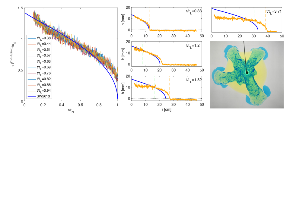
Figure 6: (a) regression of the blue-channel intensity during the non-lubricated interval ($t<t_{L}$) to the thickness solution of a non-lubricated GC (—) to get $a_{c=\mbox{blue}}$. (b) Thickness evolution of a lubricated GC (experiment #1, —) and of the corresponding non-lubricated GC (—). Grid lines mark the measured $r_{N}$ (- - -) and $r_{L}$ (- - -). (c) High lubrication experiment ($\mathscr{Q}\approx 0.2,\mathscr{M}\approx 7500$) leads to emergence of radial streams.

IV Discussion

We assumed that in the flow experiments the dominant deformation mechanism of our xanthan solutions is viscous. To confirm this we estimate the Debora number $De=\lambda/T$, where $\lambda\approx 0.1\,$s is the elastic relaxation time for 1% solutions (Stokes et al., 2011) and $T=\pi r^{2}h\rho/Q$ is the characteristic timescale of the flow. Having $h\approx 1$ cm, $Q/\rho\approx 0.5-5$ cm³/s, and using $r_{N}(t_{L})\approx 10-20$ cm for the radius (Figure 2), the smallest timescale we obtain is $T\approx 60$ s, implying $De\approx 0.0017$ and negligible elastic deformation. The radius where elasticity may become important ($De\approx 1$) is $r\approx 4$ mm, which is the radius of the nozzle. The relaxation time of 2% solutions is larger than $\lambda$, but even if it is tenfold larger, $De$ would still be low.

During the non-lubricated interval we measure faster evolution of the front of the 2% Xanthan solution than the prediction of Sayag and Worster (2013). This inconsistency may arise due to a more intense polymer entanglement in the 2% solution than in the 1% solution (the storage modulus of the former is $\sim 3$ times larger than of the latter, Martín-Alfonso et al., 2018). Consequently, one process that could lead to a faster propagation and be more substantial in the 2% solutions is wall slip at the fluid-solid interface, potentially through adhesive failure of the polymer chains at the solid surface or through cohesive failure due to disantanglement of chains in the bulk from chains adsorbed at the wall (Brochard and Gennes, 1992). Such mechanisms would turn the theoretically assumed no-slip condition invalid.

Although we did not calculate the thickness of the lubricating fluid, the true-color images and the transmitted red-light intensity imply that it has a complex spatiotemporal structure. In particular, the thickness is non-monotonic, containing spikes of 50% reduction in the transmission that appear to move downstream with the flow (Figure 5). This structure may arise due to roughness of the non-Newtonian fluid free surface, which may imply the presence of a yield stress. Alternatively, an instability of the fluid-fluid interface may lead to the growth of finite-amplitude thickness spikes.

The transition to the lubricated interval coincides with the growth of a non-axisymmetric component of the fronts and translation of the GCs geometric center. However, as the GC evolves these quantities appear to become confined and attenuated (Figure 3d), implying that the flow remains axisymmetric to leading order. This apparent stability may be associated with the substantially lower lubrication flux compared with the flux of the top non-Newtonian fluid. Our hypothesis is reinforced by preliminary experiments with larger $\mathscr{Q}$, which indicate breakdown of axisymmetry and the development of finger-like patterns in both the lubricating and non-lubricating flows (Figure 6c).

V Conclusions

Lubricated GCs are controlled by complex interactions between two fluid layers. The lower, lubrication layer modifies the friction between the substrate and the top layer, which in turn applies stresses that affect the distribution of the lubricating layer. The resulted flow can vary dramatically from non-lubricated GCs.

In our experiments at low flux ratio ($\mathscr{Q}<0.06$) we find that the two fronts follow a power-law evolution with similar exponents as their corresponding non-lubricated GCs, but they propagate faster than the fronts of non-lubricated GC. Specifically, following a transient acceleration during the lubricated stage, the front $r_{N}$ of the non-Newtonian fluid evolves with the same exponent $(2n+2)/(5n+3)$ as a non-lubricated PL fluid, but with a larger intercept. The front $r_{L}$ of the lower lubricating fluid evolves with the same exponent $1/2$ as Newtonian GCs, but with an intercept that appears sensitive to the properties of the overlaying non-Newtonian fluid. Unlike non-lubricated GCs, the radial distribution of the thickness of the non-Newtonian fluid in the lubricated region is nearly uniform, whereas that of the lubricating fluid appears to be nonmonotonic with localised spikes. Nevertheless, the fronts of the two fluids remain axisymmetric throughout the flow, with a weak non-axisymmetric component that relaxes or remains confined.

We believe that axisymmetric models can provide accurate predictions of these flows, to leading order. However, preliminary experiments with $\mathscr{Q}>0.06$ reveal strong symmetry breaking of the circular fronts and a transition to stream-like flow, implying that for a sufficiently large $\mathscr{Q}$ the axisymmetric fronts can turn unstable. The experiments and analysis we present may provide new insights into the rich phenomenology in potentially dynamically similar systems such as ice-sheet systems coupled with hydrological networks.