The open supersymmetric Haldane–Shastry spin chain and its associated motifs

Abstract

We study the open version of the $\mathrm{su}(m|n)$ supersymmetric Haldane–Shastry spin chain associated to the $BC_{N}$ extended root system. We first evaluate the model’s partition function by modding out the dynamical degrees of freedom of the $\mathrm{su}(m|n)$ supersymmetric spin Sutherland model of $BC_{N}$ type, whose spectrum we fully determine. We then construct a generalized partition function depending polynomially on two sets of variables, which yields the standard one when evaluated at a suitable point. We show that this generalized partition function can be written in terms of two variants of the classical skew super Schur polynomials, which admit a combinatorial definition in terms of a new type of skew Young tableaux and border strips (or, equivalently, extended motifs). In this way we derive a remarkable description of the spectrum in terms of this new class of extended motifs, reminiscent of the analogous one for the closed Haldane–Shastry chain. We provide several concretes examples of this description, and in particular study in detail the $\mathrm{su}(1|1)$ model finding an analytic expression for its Helmholtz free energy in the thermodynamic limit.

1 Introduction

Recent experiments involving trapped ions and optical lattices of ultracold Rydberg atoms have made it possible to simulate spin chains and low-dimensional lattice models with long-range interactions, leading to a renewed interest in this type of fundamental quantum systems KCIKD09 ; GL14 ; JLHHZ14 ; RGLSS14 ; SZFHC15 ; HGCK16 . The quintessential example of these models is the spin $1/2$ chain independently introduced by Haldane Ha88 and Shastry Sh88 , in which the spins are uniformly arranged on a circle and the spin-spin interactions decay as the square of their inverse (chord) distance. The relevance of this model for theoretical and mathematical physics cannot be understated. Indeed, its importance in condensed matter physics is well known, as one of the simplest models whose elementary (spinon) excitations Ha91 ; Ha93 can be naturally regarded as anyons in the framework of Haldane’s fractional statistics Ha91b . It has also found numerous applications in such fundamental fields as the quantum Hall effect AI94 ; BK09 , the theory of long-range magnetism  HGCK16 , or quantum transport in mesoscopic systems BR94 ; Ca95 , to name only a few. More recently, it has been found that the ground state of the $\mathrm{su}(n)$ generalization of the Haldane–Shastry (HS) chain can be expressed in terms of chiral correlators of suitable primary fields of the $\mathrm{su}(n)$ Wess–Zumino–Novikov–Witten model at level 1, a result that has been extended to similar models with long-range interactions CS10 ; NCS11 ; BQ14 ; TNS14 .

From a more mathematical standpoint, two key properties set the HS chain apart from other integrable one-dimensional models, namely its close connection with a spin dynamical model and its Yangian symmetry even for a finite number of sites. Indeed, the HS chain can be obtained from the spin Sutherland model Su72 ; HH92 in the strong interaction limit, through a mechanism usually known as Polychronakos’s freezing trick Po93 ; Po94 . In essence, as the parameter $a$ governing the strength of the spin-spin interaction in the spin Sutherland model goes to infinity its eigenfunctions become increasingly peaked at the coordinates of the equilibrium positions of the Sutherland scalar potential, which coincide with the HS chain sites. Thus in this limit the dynamical and spin degrees of freedom effectively decouple, and the latter are governed by the HS Hamiltonian. This connection can be used to compute in closed form the partition function of the HS chain as the $a\to\infty$ limit of the quotient of the partition functions of the spin and scalar Sutherland dynamical models FG05 . In fact, this non-standard method for evaluating the partition function can be readily applied to other spin chains of HS type with rational Po94 ; BFGR08epl or hyperbolic FI94 ; BFGR10 interactions, known respectively as the Polychronakos–Frahm (PF) and Frahm–Inozemtsev (FI) chains and related to the integrable spin Calogero Ca71 ; MP93 and Inozemtsev In96 dynamical models. The latter method has also been extended to the $\mathrm{su}(m|n)$ supersymmetric versions of the HS Ha93 ; BB06 and PF BUW99 ; BB09 chains, in which each site is occupied by either an $\mathrm{su}(m)$ boson or an $\mathrm{su}(n)$ fermion.

The second characteristic feature of the HS chain (including its supersymmetric version) is its invariance under the Yangian quantum group $Y(\mathrm{gl}(n))$ (for $\mathrm{su}(n)$ spin) even for a finite number of sites HHTBP92 ; BGHP93 , which is in fact at the root of many of the model’s most salient properties. To begin with, a direct consequence of the Yangian symmetry is the high degeneracy of the spectrum, a fact already noted in Haldane’s original paper. On a more quantitative level, the model’s eigenstates can be classified using certain representations of the Yangian labeled by a class of skew Young diagrams known as border strips, whose dimension coincides with the number of their associated semistandard Young tableaux KKN97 ; NT98 . As it turns out, these border strips are in a one-to-one correspondence with sequences of the binary digits 0 and 1, which essentially coincide with Haldane’s motifs HHTBP92 . It should be noted, however, that this elegant description of the spectrum in terms of motifs (or border strips) and their associated Young tableaux cannot be obtained directly from the model’s partition function. Indeed, to derive this description it is necessary to infer a generalized partition function depending polynomially on certain auxiliary variables, which reduces to the standard one when evaluated at a suitable point. It is then shown that this generalized partition function can be expressed in terms of skew Schur polynomials associated to border strips. Using the combinatorial definition of the latter polynomials, it is then immediate to assign an energy to each border strip and to relate its degeneracy to the number of associated Young tableaux (see, e.g., BBHS07 ; BBH10 ). This is seen to imply that the spectrum of the supersymmetric HS chain coincides with that of a classical vertex model with local interactions and a suitably chosen energy function. Again, the Yangian symmetry and its consequences described above also hold for the supersymmetric PF chain HB00 ; BBH10 . Remarkably, this description of the spectrum of the supersymmetric HS and PF chains holds with minor changes if we add to the Hamiltonian of these models a chemical potential term EFG12 ; FGLR18 . As shown in the latter references, this makes it possible to compute the thermodynamic functions of these models and analyze their critical behavior using the (inhomogeneous) transfer matrix method.

The spin chains of HS type discussed so far are connected to the root system of the simple Lie algebra $A_{N-1}$, since in all of them the spin-spin interactions depend only on the difference of the site coordinates. The same is true for the corresponding spin dynamical models of Calogero–Sutherland type, whose interaction potential is a function of the difference of the particles’ coordinates. Since the pioneering work of Olshanetsky and Perelomov OP83 , it has been known that it is possible to obtain integrable variants of the (scalar) Calogero–Sutherland models of $A_{N-1}$ type associated to the extended root systems of all the classical simple Lie algebras. It is then relatively straightforward to construct (supersymmetric) spin dynamical models associated to the non-exceptional root systems $BC_{N}$, $B_{N}$ and $D_{N}$, each of which gives rise to a corresponding spin chain through the freezing trick (see, e.g., BPS95 ; Ya95 ; FGGRZ03 ; EFGR05 ; BFGR09 ; BFG09 ; BFG11 ; BFG13 ). Of these three types of models the $BC_{N}$ ones have received the most attention, in part because they contain one or two more free parameters than the $B_{N}$ and $D_{N}$ ones, respectively. In particular, a reduction of the HS chain of $BC_{N}$ type (in which the spin reversal operators are replaced by the identity) has recently appeared as the parent Hamiltonian of certain infinite matrix product states constructed from the chiral correlators of primary fields of a boundary conformal field theory TS15 ; BFG16 .

On the other hand, the spin Calogero–Sutherland models of $BC_{N}$ type and their associated spin chains have not been studied to the same extent as their $A_{N-1}$ counterparts. Most notably, although the partition functions of both the PF BFGR09 and HS EFGR05 chains of $BC_{N}$ type have been computed in closed form (the latter only in the non-supersymmetric case), till very recently a description of their spectrum in terms of suitable motifs has been conspicuously lacking. For the PF chain such a description has just been provided in Ref. BS20 , building on previous work on the generalized partition function of this model BD17 . More precisely, each $A_{N-1}$-type motif splits into up to $N+1$ “branched motifs” with different energies, whose degeneracies can be obtained through a combinatorial formula.

The aim of this paper is to derive a complete description of the spectrum of the supersymmetric Haldane–Shastry chain of $BC_{N}$ type in terms of suitable motifs. This model can be regarded as an open version of the original (closed) HS chain, since its sites lie on the upper unit half-circle and each spin interacts with the remaining ones and with their reflections with respect to the circle’s horizontal diameter. Our approach significantly differs from that of Refs. BD17 ; BS20 , since the structure of the partition functions of the PF and HS chains is considerably different. In particular, while the generalized partition function of the PF chain is a straightforward generalization of a Rogers–Szegő multivariate polynomial, this is not the case for the HS chain. Our starting point is instead a different ansatz for the generalized partition function of the supersymmetric HS chain of $BC_{N}$ type, which reduces to the standard one when evaluated at a suitable point. This generalized partition function is then expressed in terms of two different variants of the classical super Schur polynomials. Remarkably, it can be shown that each of these polynomials can be associated to an extended border strip of length $N+1$ (or, equivalently, motif of length $N$), where $N$ is the number of sites, and its energy expressed in terms of the model’s dispersion relation in the usual way. The crucial difference with the $A_{N-1}$ case is that the allowed skew Young tableaux for these extended border strips must have their last box filled by a fixed integer depending on the number of fermionic and bosonic degrees of freedom. In this way we obtain a simple description of the spectrum in terms of extended motifs and restricted Young tableaux, with a combinatorial expression for the degeneracy of the corresponding multiplets.

The above result has important consequences in connection with some of the model’s fundamental properties, as we shall now discuss. To begin with, the existence of a motif-based description of the spectrum strongly suggests that the twisted Yangian symmetry possessed by the non-supersymmetric open HS chain BPS95 is also present in its supersymmetric extension studied here. Another consequence of such a description, together with the simplicity of the model’s dispersion relation FG15 , is the huge degeneracy of the spectrum, which we have numerically checked for a relatively large number of particles taking advantage of our simple characterization of the spectrum. We have also applied this characterization to find a simple formula for the partition function of the $\mathrm{su}(1|1)$ model for an arbitrary number of spins, from which we have derived a closed-form expression for its free energy per site in the thermodynamic limit. For the general $\mathrm{su}(m|n)$ chain, our motif-based description of the spectrum can be regarded as the first step towards determining the model’s thermodynamics via the inhomogeneous transfer matrix method successfully applied to its $A_{N-1}$ counterpart FGLR18 .

This paper is organized as follows. In Section 2 we introduce the model and outline the computation of its partition function applying Polychronakos’s freezing trick. This computation is carried out in detail in Section 3, after determining the spectrum of the $\mathrm{su}(m|n)$ spin Sutherland model. Section 4 is devoted to a brief review of the definition of the classical skew super Schur polynomials and their connections with border strips and skew Young tableaux. In Section 5 we construct a generalized partition function for the model, which is then applied in the following section to deduce a complete description of the spectrum in terms of extended border strips and restricted supersymmetric Young tableaux. We provide some specific examples of this general result in Section 7, where we also study in detail the $\mathrm{su}(1|1)$ model and its thermodynamics. Finally, in Section 8 we present our conclusions and point out several avenues for further research suggested by our results.

2 The model

The open ($BC_{N}$-type) supersymmetric Haldane–Shastry spin chain describes an array of $N$ particles, which can be either bosons or fermions, lying on the upper unit half-circle at fixed angles $2\theta_{i}\in(0,\pi)$ determined by the $N$ roots $\theta_{i}$ of the equation

$$P^{(\beta-1,\beta^{\prime}-1)}_{N}(\cos 2\theta)=0.$$ (2.1)

Here $\beta$ and $\beta^{\prime}$ are two positive parameters, and $P^{(\beta-1,\beta^{\prime}-1)}_{N}$ is a Jacobi polynomial of degree $N$. Note that the chain sites $\mathrm{e}^{2\mathrm{i}\,\theta_{j}}$ (with $j=1,\dots,N$) are not uniformly spaced unless the pair $(\beta,\beta^{\prime})$ takes the values specified in Table 1.

$(\beta,\beta^{\prime})$	$\theta_{j}$
$(1/2,1/2)$	$\pi(j-1/2)/2N$
$(3/2,1/2)$	$\pi j/(2N+1)$
$(3/2,3/2)$	$\pi j/(2N+2)$

Table 1: Values of the parameters $(\beta,\beta^{\prime})$ for which the points $\mathrm{e}^{\mathrm{i}\theta_{j}}$ with $j=1,\dots,N$ determined by Eq. (2.1) are uniformly spaced (the corresponding values of $\theta_{j}$ are listed in the second column).

If $m$ and $n$ respectively denote the number of bosonic and fermionic internal degrees of freedom, the Hilbert space of the system is the linear space ${\mathcal{S}}^{(m|n)}=\otimes_{i=1}^{N}{\mathcal{S}}_{i}^{(m|n)}$ with ${\mathcal{S}}_{i}^{(m|n)}={\mathbb{C}}^{m+n}$ spanned by the basis vectors

$$|s_{1}\cdots s_{N}\rangle:=|s_{1}\rangle\otimes\cdots\otimes|s_{N}\rangle,\qquad 1\leqslant s_{i}\leqslant m+n.$$ (2.2)

In order to define the bosonic and fermionic degrees of freedom in ${\mathbb{C}}^{m+n}$, consider two complementary subsets $B,F\subset\{1,\ldots,m+n\}$ with $B=\{b_{1},\ldots,b_{m}\}$ and $F=\{f_{1},\ldots,f_{n}\}$, where $b_{1}<b_{2}<\cdots<b_{m}$ and $f_{1}<f_{2}<\cdots<f_{n}\,$. In what follows we shall accordingly call the single particle state $|s_{i}\rangle$ bosonic if $s_{i}\in B$ or fermionic if $s_{i}\in F$.

Setting $\theta^{\pm}_{ij}:=\theta_{i}\pm\theta_{j}$, the model’s Hamiltonian can be taken as

$$H=\frac{1}{8}\sum_{i\neq j}\bigg{(}\frac{1-S_{ij}}{\sin^{2}\theta_{ij}^{-}}+\frac{1-\widetilde{S}_{ij}}{\sin^{2}\theta_{ij}^{+}}\bigg{)}+\frac{1}{8}\sum_{i}\left(\frac{\beta}{\sin^{2}\theta_{i}}+\frac{\beta^{\prime}}{\cos^{2}\theta_{i}}\right)\big{(}1-S_{i}\big{)},$$ (2.3)

where the Latin indices (as in the sequel, unless otherwise stated) run from $1$ to $N$ and we have set

$$\widetilde{S}_{ij}:=S_{i}S_{j}S_{ij}\,.$$ (2.4a)

The Hamiltonian (2.3) depends on two types of operators implementing the long-range interaction among the spins. More precisely, the supersymmetric spin permutation operators $$S_{ij}=S_{ji}$$ are defined by

$$S_{ij}|\cdots s_{i}\cdots s_{j}\cdots\rangle:=(-1)^{\nu(s_{i},\dots,s_{j})}|\cdots s_{j}\cdots s_{i}\cdots\rangle\,,$$ (2.4b)

where $$\nu(s_{i},\dots,s_{j}) 0 1 s_{i},s_{j}\in B s_{i},s_{j}\in F s_{k} i+1\leqslant k\leqslant j-1 S_{i}$$ is (respectively ) if (respectively ), and is otherwise equal to the number of fermionic spins with . Likewise, the spin reversal operators are defined by

$$S_{i}|\cdots s_{i}\cdots\rangle:=\lambda_{\varepsilon\varepsilon^{\prime}}(s_{i})|\cdots\imath(s_{i})\cdots\rangle\,,$$ (2.4c)

where $\varepsilon,\varepsilon^{\prime}=\pm$ are two fixed signs and $\lambda_{\varepsilon\varepsilon^{\prime}}(s_{i})$ is $\varepsilon$ for bosons (i.e, for $s_{i}\in B$) and $\varepsilon^{\prime}$ for fermions (i.e., $s_{i}\in F$). Here $\imath$ is in general any nontrivial involution leaving invariant the bosonic and fermionic sectors, i.e., $\imath^{2}=I\neq\imath$, $\imath(B)=B$ and $\imath(F)=F$. Assuming that $\imath$ has at most one fixed point in each sector, we shall fix its action by setting

$$\imath(b_{\alpha}):=b_{m+1-\alpha}\,,\qquad\imath(f_{\beta}):=f_{n+1-\beta}\,,$$

where, as in the sequel, the Greek indices are assumed to label the elements of the sets $B$ and $F$ so that they run from $1$ to $m$ for bosons and from $1$ to $m+n$ for fermions unless otherwise stated. The existence of fixed points of the involution $\imath$ obviously depends on the parity of the integers $m$ and $n$. Indeed, there is a bosonic (respectively fermionic) fixed point if and only if $m$ is odd (resp. $n$ is odd). One can intuitively think of $\imath$ as reversing the spin of a site, by simply relabeling the bosonic degrees of freedom according to $b_{\alpha}\mapsto b_{\alpha}^{\prime}:=\alpha-(m+1)/2$ or the fermionic ones according to $f_{\beta}\mapsto f_{\beta}^{\prime}:=\beta-(n+1)/2$. (In other words, $\big{[}\imath(b_{\alpha})]^{\prime}=b_{m+1-\alpha}^{\prime}=m+1-\alpha-\frac{1}{2}(m+1)=\frac{1}{2}(m+1)-\alpha=-b_{\alpha}^{\prime}$, and similarly for fermions.)

Remark 1.

As mentioned in the Introduction, the model (2.3) can be regarded as an open version of the (supersymmetric) Haldane–Shastry chain. More precisely, the chain sites $z_{j}:=\mathrm{e}^{2\mathrm{i}\theta_{j}}$ lie on the upper unit circle, and the spin at $z_{j}$ interacts not only with the remaining spins at $z_{k}$ (with $k\neq j$) but also with their reflections with respect to the real axes $\bar{z}_{k}$. Moreover, the strength of these interactions is equal to the inverse square of the distance between $z_{j}$ and the points $z_{k}$ and $\bar{z}_{k}$, respectively. Writing the last term in Eq. (2.3) as

$$\frac{1}{8}\sum_{i}\bigg{(}\frac{\beta-\beta^{\prime}}{\sin^{2}\theta_{i}}+\frac{4\beta^{\prime}}{\sin^{2}(2\theta_{i})}\bigg{)}(1-S_{i})$$

shows that the Hamiltonian (2.3) is obviously related to the $BC_{N}$ extended root system with elements $\theta_{ij}^{\pm}$, $\theta_{i}$ and $2\theta_{i}$, with $1\leqslant i<j\leqslant N$. Note also in this respect that the operators $S_{ij}$ and $S_{i}$ obey the algebraic relations

$$S_{ij}^{2}=I\,,\qquad S_{ij}S_{jk}=S_{ik}S_{ij}=S_{jk}S_{ik}\,,\qquad S_{ij}S_{kl}=S_{kl}S_{ij}\,,$$ (2.5a)

$$S_{i}^{2}=I\,,\qquad S_{i}S_{j}=S_{j}S_{i}\,,\qquad S_{ij}S_{k}=S_{k}S_{ij}\,,\qquad S_{ij}S_{j}=S_{i}S_{ij}\,,$$ (2.5b)

where the indices $i,j,k,l$ take distinct values in the range $1,\dots,N$, and thus generate an algebra isomorphic to the group algebra of the $BC_{N}$ Weyl group.

The partition function of the chain (2.3) was evaluated in Ref. EFGR05 in the purely bosonic $(n=0)$ or purely fermionic ($m=0$) cases applying Polychronakos’s freezing trick Po93 to the spin Sutherland model of $BC_{N}$ type Ya95 . This method can be easily generalized to the genuinely supersymmetric case $mn\neq 0$, as we shall explain in the next section. More precisely, the Hamiltonian of the $\mathrm{su}(m|n)$ spin Sutherland model is defined by

$$H_{\mathrm{spin}}=-\Delta+a\sum_{i\neq j}\!\left(\frac{a-S_{ij}}{\sin^{2}x_{ij}^{-}}+\frac{a-\widetilde{S}_{ij}}{\sin^{2}x_{ij}^{+}}\right)\\ +\sum_{i}\!\left(\frac{b(b-S_{i})}{\sin^{2}x_{i}}+\frac{b^{\prime}(b^{\prime}-S_{i})}{\cos^{2}x_{i}}\right),$$ (2.6)

where $a,b,b^{\prime}$ are real parameters greater than $1/2$, $x_{ij}^{\pm}:=x_{i}\pm x_{j}$, $\Delta:=\sum_{i}\partial_{x_{i}}^{2}$, and $S_{ij}$, $S_{i}$ and $\widetilde{S}_{ij}$ are defined by Eqs. (2.4). The particles can be regarded as distinguishable and confined to the interval $(0,\pi/2)$ due to the inverse-square singularities at the hyperplanes $x_{ij}^{\pm}=k\pi$ and $x_{i}=k\pi/2$ with $k\in{\mathbb{Z}}$. We can thus take the system’s configuration space as

$$C^{\prime}=\{\mathbf{x}:=(x_{1},\dots,x_{N})\in{\mathbb{R}}^{N}:0<x_{1}<x_{2}<\cdots<x_{N}<\pi/2\}\,,$$

with corresponding Hilbert space ${\mathcal{H}}^{\prime}=L^{2}(C^{\prime})\otimes{\mathcal{S}}^{(m|n)}$. The scalar version of the Hamiltonian (2.6) is obtained by replacing the supersymmetric spin exchange and reversal operators by the identity, namely

$$H_{\mathrm{sc}}=-\Delta+a(a-1)\sum_{i\neq j}\!\bigg{(}\frac{1}{\sin^{2}x_{ij}^{-}}+\frac{1}{\sin^{2}x_{ij}^{+}}\bigg{)}+\sum_{i}\!\bigg{(}\frac{b(b-1)}{\sin^{2}x_{i}}+\frac{b^{\prime}(b^{\prime}-1)}{\cos^{2}x_{i}}\bigg{)},$$ (2.7)

which acts on the Hilbert space $L^{2}(C^{\prime})$. Note that $H_{\mathrm{sc}}$ coincides with the dynamical Hamiltonian (2.6) for the choices $(m|n)=(1|0)$ and $\varepsilon=+1$ under the canonical identification $L^{2}(C^{\prime})\otimes{\mathcal{S}}^{(1|0)}\cong L^{2}(C^{\prime})\otimes{\mathbb{C}}\cong L^{2}(C^{\prime})\,$.

Setting $b=a\beta$, $b^{\prime}=a\beta^{\prime}$ we obviously have

$$H_{\mathrm{spin}}=H_{\mathrm{sc}}+8\kern 1.0ptaH(\mathbf{x})=-\Delta+a^{2}U(\mathbf{x})+O(a)\,,$$

where $H(\mathbf{x})$ is obtained from the spin chain Hamiltonian (2.3) replacing the fixed sites $\theta_{i}$ by the dynamical variables (coordinates) $x_{i}$ and

$$U(\mathbf{x})=\sum_{i\neq j}\left(\frac{1}{\sin^{2}x_{ij}^{-}}+\frac{1}{\sin^{2}x_{ij}^{+}}\right)+\sum_{i}\!\left(\frac{\beta^{2}}{\sin^{2}x_{i}}+\frac{\beta^{\prime 2}}{\cos^{2}x_{i}}\right).$$

As $a$ grows to infinity the particles tend to freeze at the coordinates of the equilibrium of the scalar potential $U(\mathbf{x})$ on the configuration space $C^{\prime}$. It can be shown that this equilibrium is unique CS02 , and its coordinates coincide with the chain sites $\theta_{i}$ OS02 . Thus in this limit the spin degrees of freedom decouple from the dynamical ones, and are governed by the Hamiltonian $H(\theta_{1},\dots,\theta_{N})=H$. It follows that when $a\gg 1$ the eigenvalues $E_{ij}$ of $H_{\mathrm{spin}}$ behave as

$$E_{ij}=E_{\mathrm{sc},i}+8\kern 1.0ptaE_{j}+o(a),$$

where $E_{\mathrm{sc},i}$ and $E_{j}$ are any two energies of the scalar Hamiltonian (2.7) and the spin chain Hamiltonian (2.3), respectively. Let us respectively denote by $Z_{\mathrm{spin}}$ and $Z_{\rm sc}$ the partition functions of the $BC_{N}$ Sutherland spin dynamical and scalar models. The partition function $Z$ of the spin chain is then given by the exact expression

$$Z(T)=\lim_{a\to\infty}\frac{Z_{\mathrm{spin}}(8\kern 1.0ptaT)}{Z_{\mathrm{sc}}(8\kern 1.0ptaT)}\,.$$ (2.8)

This is, in essence, Polychronakos’s freezing trick as applied to the chain (2.3).

3 Partition function

3.1 Auxiliary operator

In view of the freezing trick formula (2.8), in order to compute the partition function of the chain (2.3) we need to determine the spectra of the spin dynamical model (2.6) and its scalar counterpart (2.7). To this end, we introduce the auxiliary operator

$$H_{\mathrm{aux}}=-\Delta+a\sum_{i\neq j}\!\left(\frac{a-P_{ij}}{\sin^{2}x_{ij}^{-}}+\frac{a-\widetilde{P}_{ij}}{\sin^{2}x_{ij}^{+}}\right)\\ +\sum_{i}\left(\frac{b(b-P_{i})}{\sin^{2}x_{i}}+\frac{b^{\prime}(b^{\prime}-P_{i})}{\cos^{2}x_{i}}\right),$$ (3.1)

where $P_{ij}$, $P_{i}$ are defined by

$$(P_{ij}f)(\ldots,x_{i},\ldots,x_{j},\ldots) =f(\ldots,x_{j},\ldots,x_{i},\ldots)\,,$$ (3.2a)

$$(P_{i}f)(\ldots,x_{i},\ldots) =f(\ldots,-x_{i},\ldots)$$ (3.2b)

and $\widetilde{P}_{ij}=P_{i}P_{j}P_{ij}$. The operators $H_{\mathrm{aux}}$, $P_{ij}$, and $P_{i}$ are assumed to act on the space $L^{2}(C)$ of square integrable functions defined on the whole open cube $C=(-\pi/2,\pi/2)^{N}\allowbreak\subset{\mathbb{R}}^{N}$. In particular, by contrast with $H_{\mathrm{sc}}$ the configuration space of the latter operators is not restricted to the ordered tuples in $C$. We shall also tacitly identify in what follows $H_{\mathrm{aux}}$ with its trivial extension $H_{\mathrm{aux}}\otimes I$ to the Hilbert space $L^{2}(C)\otimes{\mathcal{S}}^{(m|n)}$.

We next define total (i.e., acting simultaneously on a particle’s coordinates and spin degrees of freedom) permutation and flip operators $\Pi_{ij}$ and $\Pi_{i}$ as

$$\Pi_{ij}=P_{ij}\otimes S_{ij},\qquad\Pi_{i}=P_{i}\otimes S_{i}.$$ (3.3)

Such operators obviously depend on $m,n$ and the signs $\varepsilon,\varepsilon^{\prime}\,$, although we shall omit these labels for the sake of conciseness. Note also that the operators $\{\Pi_{ij},\Pi_{i}\}$, as well as their spin coordinate counterparts defined in Eqs. (2.4) and (3.2), provide a realization of the Weyl group of $BC_{N}$ type. For fixed values of $m,n$ and $\varepsilon,\varepsilon^{\prime}$, let us denote by $\Lambda$ the supersymmetric projector onto states totally symmetric under the action of both $\Pi_{ij}$ and $\Pi_{i}$. The key observation at this point is that the operator $H_{\mathrm{spin}}:{\mathcal{H}}^{\prime}\to{\mathcal{H}}^{\prime}$ can be shown to be unitarily equivalent to its symmetric extension under $\Pi_{ij}$ and $\Pi_{i}$ to the space ${\mathcal{H}}:=L^{2}(C)\otimes{\mathcal{S}}^{(m|n)}$ EFGR05 ; BFG11 . With a slight notational abuse, we shall henceforth identify both operators and thus study the action of the spin dynamical Hamiltonian $H_{\mathrm{spin}}$ in the Hilbert space $\Lambda({\mathcal{H}})$, instead of the original one ${\mathcal{H}}^{\prime}=L^{2}(C^{\prime})\otimes{\mathcal{S}}^{(m|n)}$. The idea is of course to derive in this way the spectrum of $H_{\mathrm{spin}}$ from that of the (essentially scalar) auxiliary operator (3.1). The spectrum of the latter operator can in turn be computed through the following standard procedure:

1. Introduce a suitable (partial) order in an appropriately chosen subset of $L^{2}(C)$ spanning a dense subspace, and construct a (Schauder, i.e., non-orthonormal) basis in which the auxiliary operator $H_{\mathrm{aux}}$ is upper triangular, and thus its eigenvalues coincide with its diagonal elements in this basis.

2. Take the direct product with ${\mathcal{S}}^{(m|n)}$ and project onto $\Lambda({\mathcal{H}})$, thus obtaining a Schauder basis of $\Lambda({\mathcal{H}})$ in which $H_{\mathrm{spin}}$ is upper triangular, with the same diagonal elements and hence eigenvalues as $H_{\mathrm{aux}}$.

To better understand the last point, note that on $\Lambda({\mathcal{H}})$ we have $\Pi_{ij}=\Pi_{i}=I$, and thus

$$P_{ij}=S_{ij}\,,\qquad P_{i}=S_{i}\,.$$

It follows that

$$H_{\mathrm{spin}}\Lambda=H_{\mathrm{aux}}\Lambda=\Lambda H_{\mathrm{aux}},$$ (3.4)

since the operators $\Lambda$ and $H_{\mathrm{aux}}$ commute (indeed, $[P_{ij},\Lambda]=[P_{i},\Lambda]=0$). In the next section we shall implement the above procedure and compute the spectrum of $H_{\mathrm{spin}}$.

3.2 Spectrum of the spin dynamical model

As explained in the last section, we begin by constructing a Schauder basis of $L^{2}(C)$ in which $H_{\mathrm{aux}}$ is upper triangular. Consider, to this end, the function

$$\phi(\mathbf{x})=\prod_{i<j}|\sin x_{ij}^{+}\sin x_{ij}^{-}|^{a}\prod_{k}|\sin x_{k}|^{b}|\cos x_{k}|^{b^{\prime}},$$ (3.5)

which is clearly an element of $L^{2}(C)$ invariant under permutations (3.2a) and reversal (3.2b) of the coordinates, i.e., $P_{ij}\phi=P_{i}\phi=\phi\,$. For any integer multiindex $\mathbf{p}=(p_{1},\ldots,p_{N})$ with $p_{i}\in{\mathbb{Z}}$ consider the set $\{u_{\mathbf{p}}\}$, where the functions $u_{\mathbf{p}}\in L^{2}(C)$ are defined by

$$u_{\mathbf{p}}(\mathbf{x}):=\mathrm{e}^{2\mathrm{i}\kern 1.0pt\mathbf{p}\cdot\mathbf{x}}\phi(\mathbf{x})\,.$$ (3.6)

Note that

$$p_{i}=p_{j}\implies P_{ij}u_{\mathbf{p}}=u_{\mathbf{p}},\qquad p_{i}=0\implies P_{i}u_{\mathbf{p}}=u_{\mathbf{p}}.$$

The subspace spanned by the elements $\{u_{\mathbf{p}}\}$ is obviously dense in $L^{2}(C)$ (since $\{\mathrm{e}^{2\mathrm{i}\kern 1.0pt\mathbf{p}\cdot\mathbf{x}}\}$ is), and we can thus construct a Schauder basis out of it by introducing an order. To do so, consider the application $\mathbf{p}\mapsto\bar{\mathbf{p}}$ defined by

$$\bar{\mathbf{p}}:=(\bar{p}_{1},\ldots,\bar{p}_{N})=(|p_{i_{1}}|,\dots,|p_{i_{N}}|)$$

where $(i_{1},\dots,i_{N})$ is a permutation of $(1,\dots,n)$ such that $\bar{\mathbf{p}}$ is nonincreasing, i.e., $\bar{p}_{i}\geqslant\bar{p}_{i+1}$ (and obviously nonnegative). We order the set of nonnegative nonincreasing multiindices using the lexicographical order $\prec$, i.e., we write $\bar{\mathbf{p}}\prec\bar{\mathbf{q}}$ if and only if the first nonzero difference $\bar{p}_{i}-\bar{q}_{i}$ is negative. We then define a partial order in the set of integer multiindices $\{\mathbf{p}\}$ by setting $\mathbf{p}\prec\mathbf{q}$ if and only if $\bar{\mathbf{p}}\prec\bar{\mathbf{q}}$. This in turn induces a partial order in $\{u_{\mathbf{p}}\}$, namely $u_{\mathbf{p}}\prec u_{\mathbf{q}}$ if and only if $\mathbf{p}\prec\mathbf{q}$. As shown in Ref. EFGR05 , the auxiliary operator $H_{\mathrm{aux}}$ is upper triangular in the basis obtained ordering $\{u_{\mathbf{p}}\}$ with any order compatible with $\prec$, with diagonal elements given by

$$(H_{\mathrm{aux}})_{\mathbf{p}\mathbf{p}}=\sum_{i}\big{(}2\bar{p}_{i}+b+b^{\prime}+2a(N-i)\big{)}^{2}\,.$$ (3.7)

Let us now turn to the second point of the procedure described at the end of the last section. To begin with, let us define the spin wave functions

$$|\mathbf{p},\mathbf{s}\rangle:=\Lambda(u_{\mathbf{p}}|\mathbf{s}\rangle)=\Lambda\bigl{(}\mathrm{e}^{2\mathrm{i}\kern 1.0pt\mathbf{p}\cdot\mathbf{x}}\phi(\mathbf{x})|\mathbf{s}\rangle\bigr{)}\,,$$

where $\mathbf{p}\in{\mathbb{Z}}^{N}$ and $|\mathbf{s}\rangle:=|s_{1},\dots,s_{N}\rangle$ is an element of the canonical spin basis (2.2) of ${\mathcal{S}}^{(m|n)}$. Since the span of the set $\{u_{\mathbf{p}}\}$ with $\mathbf{p}\in{\mathbb{Z}}^{N}$ is dense in $L^{2}(C)$, the set of vectors $\{|\mathbf{p},\mathbf{s}\rangle\}$ with $\mathbf{p}\in{\mathbb{Z}}^{N}$ and $s_{i}\in\{1,\dots,m+n\}$ obviously spans a dense subspace of $\Lambda({\mathcal{H}})$. These vectors are however not linearly independent, since from the identities

$$\Pi_{ij}|\mathbf{p},\mathbf{s}\rangle=\Pi_{i}|\mathbf{p},\mathbf{s}\rangle=|\mathbf{p},\mathbf{s}\rangle$$

it follows that the state $|\mathbf{p},\mathbf{s}\rangle$ is invariant under simultaneous permutations and reversals of the quantum numbers $(\mathbf{p},\mathbf{s})$. For this reason, in order to construct a basis from the set $\{|\mathbf{p},\mathbf{s}\rangle\}$ we can assume without loss of generality that $p_{i}\in{\mathbb{N}}\cup\{0\}$ and $p_{i}\geqslant p_{i+1}$ for all $i$. Similarly, if $p_{i}=p_{i+1}$ we can obviously take (for instance) $s_{i}\leqslant s_{i+1}$ for bosons and $s_{i}<s_{i+1}$ for fermions. Indeed, if $s_{i}=s_{i+1}\in F$ we have

$$|\mathbf{p},\mathbf{s}\rangle=\Pi_{i,i+1}|\mathbf{p},\mathbf{s}\rangle=-|\mathbf{p},\mathbf{s}\rangle\implies|\mathbf{p},\mathbf{s}\rangle=0\,.$$

Finally, $|\mathbf{p},\mathbf{s}\rangle=0$ when $p_{i}=0$ and $s_{i}\in B$ is a fixed point of the involution (“spin reversal”) $\imath$ when $\varepsilon=-1$, or $s_{i}\in F$ is a fixed point of $\imath$ when $\varepsilon^{\prime}=-1$. Indeed, in the first case we have

$$\Pi_{i}|\mathbf{p},\mathbf{s}\rangle=|\mathbf{p},\mathbf{s}\rangle=\varepsilon|\mathbf{p},\mathbf{s}\rangle=-|\mathbf{p},\mathbf{s}\rangle,$$

and similarly in the second one. With this observation in mind, we define the sets $B_{\varepsilon}\subset B$ and $F_{\varepsilon^{\prime}}\subset F$ by

$$B_{\varepsilon}:=\{b_{1},\ldots,b_{m_{\varepsilon}}\}\,,\qquad F_{\varepsilon^{\prime}}:=\{f_{1},\ldots,f_{n_{\varepsilon^{\prime}}}\}\,,$$

with

$$m_{\varepsilon}:=\frac{1}{2}\big{(}m+\varepsilon\pi(m)\big{)},\qquad n_{\varepsilon^{\prime}}:=\frac{1}{2}\big{(}n+\varepsilon^{\prime}\pi(n)\big{)}.$$

It then follows from the above remarks that when $p_{i}=0$ we can restrict without loss of generality the corresponding spin component $s_{i}$ to $B_{\varepsilon}\cup F_{\varepsilon^{\prime}}$. Summarizing, we have found the following necessary conditions on the quantum numbers $(\mathbf{p},\mathbf{s})$ for the set $\{|\mathbf{p},\mathbf{s}\rangle\}$ to be a basis of $\Lambda({\mathcal{H}})$.

1. The integer multiindex $p=(p_{1},\ldots,p_{N})$ is nonnegative and nonincreasing, i.e., $p_{i}\in{\mathbb{N}}\cup\{0\}$ and $p_{i}\geqslant p_{i+1}\,$ for all $i$.

2. If $p_{i}=p_{i+1}$ then $s_{i}\geqslant s_{i+1}$ if $s_{i}\in B$ and $s_{i}>s_{i+1}$ if $s_{i}\in F$.

3. If $p_{i}=0$ then $s_{i}\in B_{\varepsilon}\cup F_{\varepsilon^{\prime}}$.

It is straightforward to show that the above conditions are actually sufficient, i.e., that they ensure the linear independence of the set $\{|\mathbf{p},\mathbf{s}\rangle\}$.

It follows from Eq. (3.4) that the action of the spin dynamical Hamiltonian $H_{\mathrm{spin}}$ is upper triangular in any basis $\mathfrak{B}$ of $\Lambda({\mathcal{H}})$ constructed from states $\{|\mathbf{p},\mathbf{s}\}\rangle$ with $(\mathbf{p},\mathbf{s})$ satisfying the above three conditions, provided that we set $|\mathbf{p},\mathbf{s}\rangle\prec|\mathbf{p}^{\prime},\mathbf{s}^{\prime}\rangle$ if and only if $\mathbf{p}\prec\mathbf{p}^{\prime}$. Indeed,

$$H_{\mathrm{spin}}|\mathbf{p},\mathbf{s}\rangle =H_{\mathrm{spin}}\Lambda\bigl{(}u_{\mathbf{p}}|\mathbf{s}\rangle\bigr{)}=\Lambda H_{\mathrm{aux}}\bigl{(}u_{\mathbf{p}}|\mathbf{s}\rangle\bigr{)}=\Lambda\bigl{(}(H_{\mathrm{aux}}u_{\mathbf{p}})|\mathbf{s}\rangle\bigr{)}$$

$$=\Lambda\Biggl{(}\,\sum_{\mathbf{p}^{\prime}\preceq\mathbf{p}}(H_{\mathrm{aux}})_{\mathbf{p}^{\prime}\mathbf{p}}u_{\mathbf{p}^{\prime}}|\mathbf{s}\rangle\!\Biggr{)}=\sum_{\mathbf{p}^{\prime}\preceq\mathbf{p}}(H_{\mathrm{aux}})_{\mathbf{p}^{\prime}\mathbf{p}}|\mathbf{p}^{\prime},\mathbf{s}\rangle,$$

where the symbol $\mathbf{p}^{\prime}\preceq\mathbf{p}$ indicates that either $\mathbf{p}^{\prime}\prec\mathbf{p}$ or $\mathbf{p}^{\prime}=\mathbf{p}$. Of course, if $\mathbf{p}^{\prime}\neq\mathbf{p}$ the quantum numbers $(\mathbf{p}^{\prime},\mathbf{s})$ need no longer satisfy conditions (B1)–(B3) above (in particular, the state $|\mathbf{p}^{\prime},\mathbf{s}\rangle$ could vanish). However, if $|\mathbf{p}^{\prime},\mathbf{s}\rangle\neq 0$ applying suitable permutations and reversals to these quantum numbers we can always write

$$|\mathbf{p}^{\prime},\mathbf{s}\rangle=\pm|\mathbf{p}^{\prime\prime},\mathbf{s}^{\prime}\rangle\,,$$

with $(\mathbf{p}^{\prime\prime},\mathbf{s}^{\prime})$ satisfying (B1)–(B3). Since the partial order $\prec$ is obviously invariant under permutations and sign reversals we obviously have $\mathbf{p}^{\prime\prime}\prec\mathbf{p}$, and therefore $|\mathbf{p}^{\prime\prime},\mathbf{s}^{\prime}\rangle\prec|\mathbf{p},\mathbf{s}\rangle$. This indeed shows that $H_{\mathrm{spin}}$ is indeed upper triangular in the basis $\mathfrak{B}$ of states $|\mathbf{p},\mathbf{s}\rangle$ satisfying conditions (B1)–(B3) and partially ordered by $\prec$, with eigenvalues

$$(H_{\mathrm{spin}})_{\mathbf{p}\mathbf{s},\mathbf{p}\mathbf{s}}=(H_{\mathrm{aux}})_{\mathbf{p}\mathbf{p}}=\sum_{i}\big{(}2p_{i}+b+b^{\prime}+2a(N-i)\big{)}^{2}=:E_{\mathbf{p}}.$$ (3.8)

Since $E_{\mathbf{p}}$ does not depend on $\mathbf{s}$, each multiindex $\mathbf{p}$ satisfying condition (B1) gives rise to an eigenvalue of $H_{\mathrm{spin}}$ whose intrinsic (or spin) degeneracy $d(\mathbf{p})$ is equal to the number of spin configurations $\mathbf{s}$ satisfying conditions (B2) and (B3).

Remark 2.

A similar argument shows that the eigenvalues of the scalar Hamiltonian $H_{\mathrm{sc}}$ are also given by Eq. (3.8), although in this case each of them has no spin degeneracy. Thus $H_{\mathrm{spin}}$ and $H_{\mathrm{sc}}$ have the same (distinct) eigenvalues, but with different degeneracies.

In order to compute the spin degeneracy of the eigenvalues of $H_{\mathrm{spin}}$, let us divide the vector $\mathbf{p}$ in “sectors” consisting of equal entries, i.e.,

$$\mathbf{p}=(\,\underbrace{\pi_{1},\dots,\pi_{1}}_{k_{1}}\,,\dots\,,\underbrace{\pi_{r},\dots,\pi_{r}}_{k_{r}})\,,$$ (3.9)

where $k_{i}$ is the number of entries with the same value $\pi_{i}$ and $\pi_{1}>\cdots>\pi_{r}\geqslant 0$ on account of condition (B1). Note that the number of sectors $r$ is always between $1$ and $N$, and that $k_{1}+k_{2}+\cdots+k_{r}=N$, i.e., $\mathbf{k}$ belongs to the set ${\mathcal{P}}_{N}$ of compositions of the integer $N$ (that is, partitions with order taken into account). The spin degeneracy $d(\mathbf{p})$ of the eigenvalue $E_{\mathbf{p}}$ depends only on the vector $\mathbf{k}=(k_{1},\ldots,k_{r})$ (i.e., on the lengths of the sectors in $\mathbf{p}$) and on the value $\pi_{r}$ of the last (smallest) distinct entry of $\mathbf{p}$. Indeed, $d(\mathbf{p})$ is obviously a product whose factors are the different ways of “filling” the spin components of $\mathbf{s}$ corresponding to each sector in $\mathbf{p}$ in accordance to conditions (B2)-(B3) above. For each of the first $r-1$ sectors we have $\pi_{i}>0$, so that condition (B3) is vacuous. Hence in this case the number of fillings is simply equal to the number of ways in which one can choose $k_{i}$ values among $m$ bosonic spins (which can appear more than once) and $n$ fermionic ones (which cannot), i.e.,

$$\sum_{l=0}^{k_{i}}\binom{m+l-1}{l}\binom{n}{k_{i}-l}=:d^{(m|n)}_{k_{i}}\,.$$ (3.10)

The same is true for the last sector when $\pi_{r}>0$. On the other hand, if $\pi_{r}=0$ we must take condition (B3) into account, and hence the number of bosonic and fermionic values available to fill the last sector of $\mathbf{p}$ is reduced respectively to $m_{\varepsilon}$ and $n_{\varepsilon^{\prime}}$. Hence the number of fillings of the last sector is in this case given by $d^{(m_{\varepsilon}|n_{\varepsilon^{\prime}})}_{k_{r}}$. Thus the intrinsic degeneracy of the eigenvalue of $H_{\mathrm{spin}}$ associated with the multiindex $\mathbf{p}$ is given by

$$d(\mathbf{p})=d_{\varepsilon\varepsilon^{\prime}}^{(m|n)}(\pi_{r},k_{r})\prod_{i=1}^{r-1}d^{(m|n)}_{k_{i}},$$ (3.11)

where $d^{(m|n)}_{k}$ is defined by Eq. (3.10) and

$$d_{\varepsilon\varepsilon^{\prime}}^{(m|n)}(\pi_{r},k_{r})=\begin{cases}d^{(m|n)}_{k_{r}},\quad&\pi_{r}>0,\\[8.0pt] d^{(m_{\varepsilon}|n_{\varepsilon^{\prime}})}_{k_{r}},&\pi_{r}=0.\end{cases}$$ (3.12)

3.3 Computation of the partition function

We are now ready to compute the partition function $Z_{\mathrm{spin}}$ of $H_{\mathrm{spin}}$ in the large coupling constant limit $a\to\infty$. To this end, given a multiindex $\mathbf{p}$ of the form (3.9) satisfying condition (B1) let us denote by

$$K_{j}:=\sum_{i=1}^{j}k_{i}$$

the partial sums of the vector $\mathbf{k}$. Setting

$$\bar{\beta}:=\frac{1}{2}(\beta+\beta^{\prime})=\frac{b+b^{\prime}}{2a}$$

and expanding Eq. (3.8) in powers of $a$ after a straightforward calculation we obtain EFGR05

$$E_{\mathbf{p}}=E_{0}+8a\sum_{j=1}^{r}\pi_{j}k_{j}\left(\,\bar{\beta}+N-K_{j-1}-(k_{j}+1)/2\right)+O(1)\,,$$

where

$$E_{0}=4a^{2}\sum_{i}(\bar{\beta}+N-i)^{2}=\frac{2}{3}\,Na^{2}\big{(}2N^{2}+3(2\bar{\beta}-1)N+6\bar{\beta}(\bar{\beta}-1)+1\big{)}$$

is the ground state energy of $H_{\mathrm{spin}}$ and $H_{\mathrm{sc}}$. Writing $q:=\mathrm{e}^{-1/T}$ and taking the limit $a\to\infty$ we thus have

$$\lim_{a\to\infty}\!q^{-E_{0}/8a}Z_{\mathrm{spin}}(8aT)=\sum_{\mathbf{k}\in{\mathcal{P}}_{N}}\,\sum_{\pi_{1}>\cdots>\pi_{r}\geqslant 0}d(\mathbf{p})\,q^{\sum_{j=1}^{r}\!\pi_{j}k_{j}\left(\,\bar{\beta}+N-K_{j-1}-(k_{j}+1)/2\right)}.$$

The latter sum can be evaluated using the formula

$$\Sigma_{l}:=\sum_{\pi_{1}>\cdots>\pi_{l}>0}q^{\sum_{j=1}^{l}\!\pi_{j}k_{j}\left(\,\bar{\beta}+N-K_{j-1}-(k_{j}+1)/2\right)}=\prod_{i=1}^{l}\frac{q^{{\mathcal{E}}(K_{i})}}{1-q^{{\mathcal{E}}(K_{i})}}\,.$$

proved in Ref. EFGR05 , where

$${\mathcal{E}}(j):=\frac{1}{2}\,j(2\kern 1.0pt\bar{\beta}+2\kern 1.0ptN-j-1)$$ (3.13)

can be interpreted as the dispersion relation of the HS chain of $BC_{N}$ type (2.3). Indeed, taking Eqs. (3.11)-(3.12) into account we easily obtain the following asymptotic expression for the partition function of the $\mathrm{su}(m|n)$ supersymmetric spin Sutherland mode of $BC_{N}$ type:

$$\lim_{a\to\infty}\!q^{-E_{0}/8a}Z_{\mathrm{spin}}(8aT) =\sum_{\mathbf{k}\in{\mathcal{P}}_{N}}\left(\prod_{i=1}^{r}d_{k_{i}}^{(m|n)}\cdot\Sigma_{r}+d_{k_{r}}^{(m_{\varepsilon}|n_{\varepsilon^{\prime}})}\prod_{i=1}^{r-1}d_{k_{i}}^{(m|n)}\cdot\Sigma_{r-1}\right)$$ (3.14)

$$=\sum_{\mathbf{k}\in{\mathcal{P}}_{N}}\left(\,\frac{d_{k_{r}}^{\kern 1.0pt(m|n)}\,q^{{\mathcal{E}}(N)}}{1-q^{{\mathcal{E}}(N)}}+d_{k_{r}}^{\kern 1.0pt(m_{\varepsilon}|n_{\varepsilon^{\prime}})}\right)\prod_{i=1}^{r-1}\frac{d_{k_{i}}^{\kern 1.0pt(m|n)}\,q^{{\mathcal{E}}(K_{i})}}{1-q^{{\mathcal{E}}(K_{i})}}\,.$$

The partition function of the scalar Sutherland model of $BC_{N}$ type was computed in Ref. EFGR05 in the same fashion (or is just obtained from the previous expression setting $m=1$, $n=0$ and $\varepsilon=+1$), with the result

$$\lim_{a\to\infty}\!q^{-E_{0}/8a}Z_{\mathrm{sc}}(8aT)=\prod_{i=1}^{N}\Big{(}1-q^{{\mathcal{E}}(i)}\Big{)}^{-1}.$$ (3.15)

The partition function $Z(T)$ of the spin chain (2.3) follows from the freezing trick formula (2.8), namely

$$Z(T)=\sum_{\mathbf{k}\in{\mathcal{P}}_{N}}F(q,\mathbf{k})\left(d^{\kern 1.0pt(m_{\varepsilon}|n_{\varepsilon^{\prime}})}_{k_{r}}+\left(d^{(m|n)}_{k_{r}}-d^{(m_{\varepsilon}|n_{\varepsilon^{\prime}})}_{k_{r}}\right)q^{{\mathcal{E}}(N)}\right)\prod_{i=1}^{r-1}d_{k_{i}}^{(m|n)},$$ (3.16)

where $\{K^{\prime}_{1},\ldots,K^{\prime}_{N-r}\}$ is the complement of the set $\{K_{1},\ldots,K_{r}\}$ in $\{1,\ldots,N\}$ (with $K^{\prime}_{1}<K^{\prime}_{2}<\cdots<K^{\prime}_{N-r}$) and

$$F(q,\mathbf{k}):=\prod_{i=1}^{r-1}q^{{\mathcal{E}}(K_{i})}\prod_{j=1}^{N-r}(1-q^{{\mathcal{E}}(K^{\prime}_{j})})\,.$$ (3.17)

4 Skew super Schur polynomials

4.1 Symmetric polynomials

We shall start by briefly reviewing some well-known properties of symmetric polynomials to fix the notation (see, e.g., Ref. Ma95 for an in-depth treatment). The complete (homogeneous) symmetric polynomial $h_{k}(\mathbf{x})$ of degree $k$ in the vector variable $\mathbf{x}:=(x_{1},\dots,x_{m})$ is defined by

$$h_{k}(\mathbf{x})=\sum_{1\leqslant j_{1}\leqslant\cdots\leqslant j_{k}\leqslant m}x_{j_{1}}\cdots x_{j_{k}}\,.$$

Likewise, the elementary symmetric polynomial $e_{k}(\mathbf{y})$ of degree $k$ in the vector variable $\mathbf{y}:=(y_{1},\dots,y_{n})$ is given by

$$e_{k}(\mathbf{y})=\sum_{1\leqslant j_{1}<\cdots<j_{k}\leqslant n}y_{j_{1}}\cdots y_{j_{k}}\,.$$

The generating functions for these polynomials are respectively

$$\prod_{i=1}^{m}\frac{1}{1-tx_{i}}=\sum_{k=0}^{\infty}h_{k}(\mathbf{x})t^{k},\qquad\prod_{i=1}^{n}(1+ty_{i})=\sum_{k=0}^{n}e_{k}(\mathbf{y})t^{k}.$$ (4.1)

From these families of symmetric polynomials we construct the polynomials (supersymmetric elementary functions) $E_{k}^{(m|n)}$ in the vector variables $\mathbf{x}=(x_{1},\ldots,x_{m})$, $\mathbf{y}=(y_{1},\ldots,y_{n})$ as

$$E^{(m|n)}_{k}(\mathbf{x},\mathbf{y})=\sum_{j=0}^{k}h_{j}(\mathbf{x})e_{k-j}(\mathbf{y}).$$ (4.2)

The generating function of these polynomials is obviously $\prod_{i=1}^{m}(1-tx_{i})^{-1}\cdot\prod_{j=1}^{n}(1+ty_{j})$. It is immediate to check that that the value of $E^{(m|n)}_{k}(\mathbf{x},\mathbf{y})$ at the point $\mathbf{x}=(1,\ldots,1)=:(1^{m})$, $\mathbf{y}=(1^{n})$ is given by

$$E^{(m|n)}_{k}(1^{m},1^{n})=\sum_{j=0}^{k}\binom{m+j-1}{j}\binom{n}{k-j}=d^{(m|n)}_{k},$$ (4.3)

where it is understood that the combinatorial number $\binom{r}{s}$ vanishes for $s>r$.

4.2 Schur polynomials

We next define the standard Schur polynomials. To this end, consider the Young diagram labeled by an integer multiindex $\lambda=(\lambda_{1},\dots,\lambda_{r})$ with $\lambda_{1}\geqslant\cdots\geqslant\lambda_{r}>0$, which by definition consists of $\lambda_{1}$ boxes in the first (top) row, $\lambda_{2}$ boxes in the second row, etc. (cf. Fig. 1). A semistandard Young tableau of shape $\lambda$ is any filling of the Young diagram $\lambda$ with natural numbers whose entries weakly increase along each row (from left to right) and strictly increase down each column. The Schur polynomial $S_{\lambda}(x_{1},\dots,x_{m})$ corresponding to the Young diagram $\lambda$ is then defined by

$$S_{\lambda}(x_{1},\dots,x_{m})=\sum_{T}x_{1}^{t_{1}}\cdots x_{m}^{\vphantom{t_{1}}t_{m}},$$ (4.4)

where $T$ is any semistandard Young tableau of shape $\lambda$ filled with the integers $\{1,\dots,m\}$ and $t_{i}$ is the number of times the integer $i$ appears in $T$. In particular, note that $e_{k}=S_{(1^{k})}$ and $h_{k}=S_{(k)}$. The polynomial $S_{\lambda}$ can be expressed in terms of either the complete or the symmetric homogeneous polynomials through the Jacobi–Trudi determinantal formulas

$$S_{\lambda}(x_{1},\dots,x_{m}) =\det\bigl{(}h_{\lambda_{i}-i+j}(x_{1},\dots,x_{m})\bigr{)}_{i,j=1}^{r}$$ (4.5)

$$=\det\bigl{(}e_{\lambda^{\prime}_{i}-i+j}(x_{1},\dots,x_{m})\bigr{)}_{i,j=1}^{s},$$

where $\lambda^{\prime}=(\lambda^{\prime}_{1},\dots,\lambda^{\prime}_{s})$ is the Young diagram conjugate to $\lambda$ (obtained exchanging the rows and columns of $\lambda$, or equivalently reflecting $\lambda$ about its main diagonal; cf. Fig. 1).

5,4,1    3,2,2,2,1

Figure 1: Young diagram of shape $\lambda=(5,4,1)$ (left) and its conjugate $\lambda^{\prime}=(3,2,2,2,1)$ (right).

More generally, a Schur polynomial can be associated to any skew Young diagram, which we define next. If $\lambda=(\lambda_{1},\dots,\lambda_{r})$ and $\mu=(\mu_{1},\dots,\mu_{s})$ are two Young diagrams such that $\mu\subset\lambda$ (i.e., $s\leqslant r$ and $\mu_{i}\leqslant\lambda_{i}$ for all $i$), we define the skew diagram $\lambda/\mu$ as the set-theoretic difference $\lambda-\mu$, obtained by removing $\mu_{i}$ boxes from the $i$-th row of $\lambda$ starting from the left. As for Young diagrams, a (semistandard) skew Young tableau of shape $\lambda/\mu$ is any filling of the skew Young diagram $\lambda/\mu$ with natural numbers which is weakly increasing along rows and strictly increasing down columns. The corresponding (skew) Schur polynomial $S_{\lambda/\mu}(x_{1},\dots,x_{n})$ is defined again by the right-hand side of Eq. (4.4), where the sum is now over skew Young tableaux of shape $\lambda/\mu$. The Jacobi–Trudi formulas for skew Schur polynomials akin to (4.5) are

$$S_{\lambda/\mu}(x_{1},\dots,x_{n}) =\det\bigl{(}h_{\lambda_{i}-\mu_{j}-i+j}(x_{1},\dots,x_{n})\bigr{)}_{i,j=1}^{r}$$ (4.6)

$$=\det\bigl{(}e_{\lambda^{\prime}_{i}-\mu^{\prime}_{j}-i+j}(x_{1},\dots,x_{n})\bigr{)}_{i,j=1}^{s}.$$

Clearly, a skew Young diagram $\lambda/\mu$ need not be a Young diagram. A particular type of skew Young diagram which in general is not a Young diagram is a border strip, i.e., a connected skew Young diagram with no $2\times 2$ blocks. The height of a border strip is defined as the number of its rows minus one, and its length as the total number of of its boxes. We shall use the notation $\langle k_{1},\ldots,k_{r}\rangle$ to refer to the border strip with $k_{i}$ boxes in the $i$-th column, numbered from right to left (cf. Fig. 2), and shall denote by $S_{\langle k_{1},\dots,k_{r}\rangle}$ the corresponding Schur polynomial. Border strips are closely related to motifs in the description of the spectrum of spin chains of Haldane–Shastry type, as we shall discuss in Section 6. This is due to the connection of these diagrams with the corresponding skew Schur polynomials labeling the irreducible representations of certain Yangian algebras KKN97 ; NT98 .

All of the above definitions can be readily extended to the $(m|n)$ supersymmetric case by suitably adapting the definition of semistandard Young tableau. More precisely, given a skew Young diagram $\lambda/\mu$, an $(m|n)$ supersymmetric Young tableau of shape $\lambda/\mu$ is a filling of $\lambda/\mu$ with the integers $1,\dots,m+n$ that is:

1. Weakly increasing along rows and strictly increasing down columns for integers in $F$.

2. Strictly increasing along rows and weakly increasing down columns for integers in $B$,

where as usual $B=(b_{1},\dots,b_{m})$, $F=(f_{1},\dots,f_{n})$ and $B\cup F=\{1,\dots,m+n\}$ (see Fig. 3 for an example).

4+1,4+1,2+3,1+2,1+1,1+1,2,1

Figure 2: The border strip $\langle 3,1,2,4,2\rangle=(5,5,5,3,2,2,2,1)/(4,4,2,1,1,1)$.

The skew super Schur polynomial $S^{(m|n)}_{\lambda/\mu}(\mathbf{x},\mathbf{y})$, where $\mathbf{x}:=(x_{1},\dots,x_{m})$ and $\mathbf{y}:=(y_{1},\dots,y_{n})$, associated with a skew Young diagram $\lambda/\mu$ is defined by

$$S^{(m|n)}_{\lambda/\mu}(\mathbf{x},\mathbf{y})=\sum_{T}x_{1}^{t_{\vphantom{f_{1}}b_{1}}}\cdots x_{m}^{t_{\vphantom{f_{1}}b_{m}}}y_{1}^{t_{f_{1}}}\cdots y_{n}^{t_{\vphantom{f_{1}}f_{n}}},$$ (4.7)

where the sum runs over all the tableaux $T$ of shape $\lambda/\mu$ filled according to the rules spelled above. We shall be mainly interested in super Schur polynomials associated with border strips $\langle k_{1},\dots,k_{r}\rangle$, which we shall denote by $S_{\langle k_{1},\dots,k_{r}\rangle}^{(m|n)}$. The function $S^{(m|n)}_{\langle k_{1},\dots,k_{r}\rangle}(\mathbf{x},\mathbf{y})$ is a homogeneous polynomial in the variables $(\mathbf{x},\mathbf{y})$ of degree equal to the length of the associated border strip. It can be conveniently expressed in terms of the supersymmetric elementary functions $E^{(m|n)}_{k}(\mathbf{x},\mathbf{y})$ introduced above by the determinantal formula HB00 ; KKN97 ; BBHS07

$$S^{(m|n)}_{\langle k_{1},\ldots,k_{r}\rangle}=\begin{vmatrix}E^{(m|n)}_{k_{r}}&E^{(m|n)}_{k_{r-1}+k_{r}}&\cdots&E^{(m|n)}_{k_{2}+\cdots+k_{r}}&E^{(m|n)}_{k_{1}+\cdots+k_{r}}\\ 1&E^{(m|n)}_{k_{r-1}}&\cdots&E^{(m|n)}_{k_{2}+\cdots+k_{r-1}}&E^{(m|n)}_{k_{1}+\cdots+k_{r-1}}\\ 0&1&\cdots&E^{(m|n)}_{k_{2}+\cdots+k_{r-2}}&E^{(m|n)}_{k_{1}+\cdots+k_{r-2}}\\ \vdots&\vdots&&\vdots&\vdots\\ 0&0&\cdots&E^{(m|n)}_{k_{2}}&E^{(m|n)}_{k_{1}+k_{2}}\\ 0&0&\cdots&1&E^{(m|n)}_{k_{1}}\end{vmatrix}.$$ (4.8)

1 & 2 3 4 4
2 3 4 5
2

Figure 3: $(3|2)$ supersymmetric Young tableau of shape $(5,4,1)$ for the choice $B=\{1,2,3\}$, $F=\{4,5\}$.

5 Generalized partition function

Let us now turn back to the study of the partition function of the supersymmetric HS chain of $BC_{N}$ type (2.3). The method we have applied in Section 3 for its computation is a generalization of that used for the $A_{N-1}$ HS chain in Refs. FG05 ; BB06 . In order to construct a representation of the partition function of the $BC_{N}$-type chain in terms of (a variant of) super Schur polynomials, we shall therefore briefly review how this is done in the $A_{N-1}$ case BBHS07 ; BBH10 .

5.1 Review of the $A_{N-1}$ case

The Hamiltonian of the $\mathrm{su}(m|n)$-supersymmetric HS chain of $A_{N-1}$ type can be taken as

$$H_{A}=\frac{1}{2}\sum_{i<j}\frac{1-S_{ij}}{\sin^{2}\xi^{-}_{ij}},\quad\xi_{i}:=\frac{i\pi}{N},\quad i=1,\dots,N,$$ (5.1)

where as usual $S_{ij}$ is the $(m|n)$-supersymmetric spin permutation operator (2.4b). Its partition function FG05 ; BBHS07 is given by

$$Z_{A}(T)=\sum_{\mathbf{k}\in{\mathcal{P}}_{N}}\prod_{i=1}^{r}d^{(m|n)}_{k_{i}}\cdot F_{A}(q,\mathbf{k}),$$ (5.2)

where

$${\mathcal{E}}_{A}(i):=i(N-i)$$ (5.3)

is the $A_{N-1}$-type dispersion relation and $F_{A}(q,\mathbf{k})$ is defined by the right-hand side of (3.17) with ${\mathcal{E}}$ replaced by ${\mathcal{E}}_{A}$. Using the properties of the skew super Schur polynomials introduced above we can define a generalized partition function of the variables $q$, $\mathbf{x}$ and $\mathbf{y}$ by

$${\mathcal{Z}}_{A}(q;\mathbf{x},\mathbf{y})=\sum_{\mathbf{k}\in{\mathcal{P}}_{N}}\prod_{i=1}^{r}E^{(m|n)}_{k_{i}}(\mathbf{x},\mathbf{y})\cdot F_{A}(q,\mathbf{k}).$$ (5.4)

It follows from Eqs. (4.3) and (5.2) that the partition function of the $A_{N-1}$-type HS chain can be expressed in terms of the generalized partition function ${\mathcal{Z}}_{A}$ as

$$Z_{A}(q)={\mathcal{Z}}_{A}(q;1^{m},1^{n}).$$ (5.5)

Since the dispersion relation ${\mathcal{E}}_{A}$ is integer valued, the function $F_{A}(q,\mathbf{k})$, and hence the generalized partition function ${\mathcal{Z}}_{A}$, is obviously a polynomial in $q$. It can be shown BBH10 that the coefficients of the expansion of ${\mathcal{Z}}_{A}$ in powers of $q$ can be expressed in terms of the skew super Schur polynomials through the remarkable formula

$${\mathcal{Z}}_{A}(q;\mathbf{x},\mathbf{y})=\sum_{\mathbf{k}\in{\mathcal{P}}_{N}}S^{(m|n)}_{\langle k_{1},\ldots,k_{r}\rangle}(\mathbf{x},\mathbf{y})\,q^{\sum_{i=1}^{r-1}{\mathcal{E}}_{A}(K_{i})}.$$ (5.6)

One of the aims of this article is to construct the corresponding expression for the $BC_{N}$ model.

5.2 The $BC_{N}$ case

Let us now turn to the partition function (3.16) of the open supersymmetric Haldane-Shastry spin chain derived in Section 3. As in the $A_{N-1}$ case, we extend this function to a generalized partition function depending on the variables ($\mathbf{x}$, $\mathbf{y}$) replacing the degeneracies $d^{(m|n)}_{k_{i}}$, $d^{(m_{\varepsilon}|n_{\varepsilon^{\prime}})}_{k_{i}}$ by the corresponding supersymmetric elementary functions $E^{(m|n)}_{k_{i}}(\mathbf{x},\mathbf{y})$, $E_{k_{i}}^{(m_{\varepsilon}|n_{\varepsilon^{\prime}})}(\mathbf{x},\mathbf{y})$. We thus arrive at the following definition of the generalized partition function in the $BC_{N}$ case:

$${\mathcal{Z}}(q;\mathbf{x},\mathbf{y}):=\sum_{\mathbf{k}\in{\mathcal{P}}_{N}}\bigg{[}E^{(m_{\varepsilon}|n_{\varepsilon^{\prime}})}_{k_{r}}(\mathbf{x},\mathbf{y})\\ +\bigg{(}E^{(m|n)}_{k_{r}}(\mathbf{x},\mathbf{y})-E^{(m_{\varepsilon}|n_{\varepsilon^{\prime}})}_{k_{r}}(\mathbf{x},\mathbf{y})\bigg{)}q^{\mathcal{E}(N)}\bigg{]}\prod_{i=1}^{r-1}E^{(m|n)}_{k_{i}}(\mathbf{x},\mathbf{y})\cdot F(q,\mathbf{k}).$$ (5.7)

From Eq. (4.3) it again follows that the partition function of the $\mathrm{su}(m|n)$ supersymmetric open HS chain (2.3) can be obtained from the generalized partition function ${\mathcal{Z}}$ by setting $\mathbf{x}=(1^{m})$, $\mathbf{y}=(1^{n})$, i.e.,

$$Z(q)={\mathcal{Z}}(q;1^{m},1^{n}).$$

Our aim is to show that this function can be expressed in terms of suitably modified ($BC_{N}$-type) skew super Schur polynomials as

$${\mathcal{Z}}(q;\mathbf{x},\mathbf{y})=\sum_{\mathbf{k}\in{\mathcal{P}}_{N}}\bigg{(}S^{(m|n)}_{\langle k_{1},\ldots,k_{r}\rangle,0}(\mathbf{x},\mathbf{y})+S^{(m|n)}_{\langle k_{1},\ldots,k_{r}\rangle,1}(\mathbf{x},\mathbf{y})q^{{\mathcal{E}}(N)}\bigg{)}q^{\sum_{i=1}^{r-1}{\mathcal{E}}(K_{i})},$$ (5.8)

where

$$S^{(m|n)}_{\langle k_{1},\ldots,k_{r}\rangle,0}=\begin{vmatrix}E^{(m_{\varepsilon}|n_{\varepsilon^{\prime}})}_{k_{r}}&E^{(m_{\varepsilon}|n_{\varepsilon^{\prime}})}_{k_{r-1}+k_{r}}&\cdots&E^{(m_{\varepsilon}|n_{\varepsilon^{\prime}})}_{k_{1}+\cdots+k_{r}}\\ 1&E^{(m|n)}_{k_{r-1}}&\cdots&E^{(m|n)}_{k_{1}+\cdots+k_{r-1}}\\ \vdots&\vdots&&\vdots\\ 0&0&\cdots&E^{(m|n)}_{k_{1}}\end{vmatrix}$$ (5.9a)

$$S^{(m|n)}_{\langle k_{1},\ldots,k_{r}\rangle,1}\\ =\begin{vmatrix}\scriptstyle E^{(m|n)}_{k_{r}}-E^{(m_{\varepsilon}|n_{\varepsilon^{\prime}})}_{k_{r}}&\scriptstyle E^{(m|n)}_{k_{r-1}+k_{r}}-E^{(m_{\varepsilon}|n_{\varepsilon^{\prime}})}_{k_{r-1}+k_{r}}&\cdots&\scriptstyle E^{(m|n)}_{k_{1}+\cdots+k_{r}}-E^{(m_{\varepsilon}|n_{\varepsilon^{\prime}})}_{k_{1}+\cdots+k_{r}}\\ \scriptstyle 1&\scriptstyle E^{(m|n)}_{k_{r-1}}&\cdots&\scriptstyle E^{(m|n)}_{k_{1}+\cdots+k_{r-1}}\\ \vdots&\vdots&&\vdots\\ \scriptstyle 0&\scriptstyle 0&\cdots&\scriptstyle E^{(m|n)}_{k_{1}}\end{vmatrix}.$$ (5.9b)

Expanding the determinants in Eqs. (5.9) along the first row and taking into account Eq. (4.8) we obtain the following equivalent expressions for the polynomials $S^{(m|n)}_{\langle k_{1},\dots,k_{r}\rangle,\alpha}$ (with $\alpha=0,1$):

$$S^{(m|n)}_{\langle k_{1},\dots,k_{r}\rangle,\alpha}=(-1)^{r-1}f_{N,\alpha}+\sum_{s=1}^{r-1}(-1)^{s-1}f_{N-K_{r-s},\alpha}S^{(m|n)}_{\langle k_{1},\dots,k_{r-s}\rangle},$$ (5.10)

with $f_{k,0}:=E^{(m_{\varepsilon}|n_{\varepsilon^{\prime}})}_{k}$ and $f_{k,1}:=E^{(m|n)}_{k}-E^{(m_{\varepsilon}|n_{\varepsilon^{\prime}})}_{k}$. Note also that we obviously have

$$S^{(m|n)}_{\langle k_{1},\ldots,k_{r}\rangle}=S^{(m|n)}_{\langle k_{1},\ldots,k_{r}\rangle,0}+S^{(m|n)}_{\langle k_{1},\ldots,k_{r}\rangle,1}.$$ (5.11)

The proof of Eq. (5.8) closely follows the argument in BB06 for the $A_{N-1}$ case. To begin with, we can rewrite Eq. (5.7) for the generalized partition function as

$${\mathcal{Z}}(q;\mathbf{x},\mathbf{y})={\mathcal{Z}}_{0}(q;\mathbf{x},\mathbf{y})+q^{{\mathcal{E}}(N)}{\mathcal{Z}}_{1}(q;\mathbf{x},\mathbf{y}),$$ (5.12)

where

$${\mathcal{Z}}_{\alpha}(q;\mathbf{x},\mathbf{y}):=\sum_{\mathbf{k}\in{\mathcal{P}}_{N}}F(q,\mathbf{k})f_{k_{r},\alpha}(\mathbf{x},\mathbf{y})\prod_{i=1}^{r-1}E^{(m|n)}_{k_{i}}(\mathbf{x},\mathbf{y})$$ (5.13)

and $F(q;\mathbf{k})$ is given by Eq. (3.17). Expanding the second product in the definition of $F$ we obtain

$$F(q,\mathbf{k})=\sum_{\mathchoice{\hbox to0.0pt{\hss$\displaystyle{\alpha_{1},\dots,\alpha_{N-r}=0}$\hss}}{\hbox to0.0pt{\hss$\textstyle{\alpha_{1},\dots,\alpha_{N-r}=0}$\hss}}{\hbox to0.0pt{\hss$\scriptstyle{\alpha_{1},\dots,\alpha_{N-r}=0}$\hss}}{\hbox to0.0pt{\hss$\scriptscriptstyle{\alpha_{1},\dots,\alpha_{N-r}=0}$\hss}}}^{1}\,(-1)^{\alpha_{1}+\cdots+\alpha_{N-r}}\,q^{\sum_{i=1}^{r-1}{\mathcal{E}}(K_{i})+\sum_{i=1}^{N-r}\alpha_{i}{\mathcal{E}}(K^{\prime}_{i})}.$$

For a given partition $\mathbf{k}=(k_{1},\dots,k_{r})\in{\mathcal{P}}_{N}$ of length $r$, the numbers

$$\{K_{1},\dots,K_{r-1},K^{\prime}_{i_{1}},\dots,K^{\prime}_{i_{l}}\}$$

(with $1\leqslant i_{1}<\cdots<i_{l}\leqslant N-r$ and $l\leqslant N-r$) are clearly the partial sums

$$\{\widehat{K}_{1},\dots,\widehat{K}_{s-1}\}$$

(excluding $\widehat{K}_{s}=N$) of another such partition $\widehat{\mathbf{k}}\in{\mathcal{P}}_{N}$ of length $s=r+l$ finer than $\mathbf{k}$. We can thus rewrite ${\mathcal{Z}}_{\alpha}$ as

$${\mathcal{Z}}_{\alpha}(q;\mathbf{x},\mathbf{y})=\sum_{\mathbf{k}\in\mathcal{P}_{N}}{\mathfrak{S}}_{\mathbf{k},\alpha}(\mathbf{x},\mathbf{y})q^{\sum_{i=1}^{r-1}\mathcal{E}(K_{i})},$$ (5.14)

where the coefficients ${\mathfrak{S}}_{\mathbf{k}}(\mathbf{x},\mathbf{y})$ are to be determined. From the previous discussion it is clear that the only partitions $\widetilde{\mathbf{k}}=(\tilde{k}_{1},\dots,\tilde{k}_{s})\in{\mathcal{P}}_{N}$ in Eq. (5.13) which contribute to the term $q^{\sum_{i=1}^{r-1}{\mathcal{E}}(K_{i})}$ in the previous sum are those coarser than $\mathbf{k}$, i.e., such that

$$\{\widetilde{K}_{1},\dots,\widetilde{K}_{s-1}\}\subset\{K_{1},\dots,K_{r-1}\}\,.$$

Defining the integers $L_{1}<\dots<L_{s-1}$ by $\widetilde{K}_{i}=K_{L_{i}}$, and noting that $\tilde{k}_{i}=\widetilde{K}_{i}-\widetilde{K}_{i-1}$ (with $\widetilde{K}_{0}:=0$) for $i=1,\dots,s-1$ and $\tilde{k}_{s}=N-\widetilde{K}_{s-1}=N-K_{L_{s-1}}$, we thus obtain

$${\mathfrak{S}}_{\mathbf{k},\alpha}=(-1)^{r-1}f_{N,\alpha}\\ +\sum_{s=2}^{r}\,\sum_{1\leqslant L_{1}<\cdots<L_{s-1}\leqslant r-1}(-1)^{r-s}f_{N-K_{L_{s-1}},\alpha}\prod_{i=1}^{s-1}E^{(m|n)}_{K_{L_{i}}-K_{L_{i-1}}},$$ (5.15)

where the first term corresponds to the partition $\widetilde{\mathbf{k}}=(N)$ of length $s=1$. We next define the integers $\ell_{i}:=L_{i}-L_{i-1}\geqslant 1$ (with $i=1,\dots,s-1$) and $L_{0}:=0$, in terms of which $L_{i}=\sum_{j=1}^{i}\ell_{j}$. Calling $p=r-L_{s-1}\geqslant 1$, it follows that $\bm{\ell}:=(\ell_{1},\dots,\ell_{s-1})$ belongs to the set ${\mathcal{P}}_{r-p}(s-1)$ of partitions (taking order into account) of the integer $r-p$. Since $p=r-\sum_{i=1}^{s-1}\ell_{i}\leqslant r-s+1$, we can rewrite Eq. (5.15) as

$${\mathfrak{S}}_{\mathbf{k},\alpha}=(-1)^{r-1}f_{N,\alpha}+\sum_{s=2}^{r}\sum_{p=1}^{r-s+1}\sum_{\bm{\ell}\in{\mathcal{P}}_{r-p}(s-1)}(-1)^{r-s}f_{N-K_{r-p},\alpha}\prod_{i=1}^{s-1}E^{(m|n)}_{K_{L_{i}}-K_{L_{i-1}}}.$$

Exchanging the sums over $s$ and $p$ and setting $s=j+1$ we obtain

$${\mathfrak{S}}_{\mathbf{k},\alpha} =(-1)^{r-1}f_{N,\alpha}$$

$$\hphantom{(-1)^{r-1}}+\sum_{p=1}^{r-1}(-1)^{p-1}f_{N-K_{r-p},\alpha}\sum_{j=1}^{r-p}(-1)^{r-p-j}\sum_{\bm{\ell}\in{\mathcal{P}}_{r-p}(j)}\prod_{i=1}^{j}E^{(m|n)}_{K_{L_{i}}-K_{L_{i-1}}}.$$

Recalling the identity

$$\sum_{j=1}^{r-p}(-1)^{r-p-j}\sum_{\bm{\ell}\in{\mathcal{P}}_{r-p}(j)}\prod_{i=1}^{j}E^{(m|n)}_{K_{L_{i}}-K_{L_{i-1}}}=S^{(m|n)}_{\langle k_{1},\dots,k_{r-p}\rangle}$$

(cf. Eq. (3.25) in Ref. BBHS07 ) and comparing with Eq. (5.10) we conclude that

$${\mathfrak{S}}_{\mathbf{k},\alpha}=S^{(m|n)}_{\langle k_{1},\dots,k_{r}\rangle,\alpha}.$$

Equation (5.8) then follows immediately from the latter relation and (5.12)-(5.14).

Remark 3.

Following Ref. BS20 , equation (5.8) can be written as

$${\mathcal{Z}}(q;\mathbf{x},\mathbf{y})=\sum_{\mathbf{k}\in{\mathcal{P}}_{N}}S^{(m|n)}_{\langle k_{1},\ldots,k_{r}\rangle}(q;\mathbf{x},\mathbf{y})q^{\sum_{i=1}^{r-1}{\mathcal{E}}(K_{i})},$$ (5.16)

where

$$S^{(m|n)}_{\langle k_{1},\ldots,k_{r}\rangle}(q;\mathbf{x},\mathbf{y})=\sum_{l=0}^{N}S^{(m|n)}_{\langle k_{1},\ldots,k_{r}|l\rangle}(\mathbf{x},\mathbf{y})q^{{\mathcal{E}}(l)}$$ (5.17a)

with

$$S^{(m|n)}_{\langle k_{1},\ldots,k_{r}|l\rangle}(\mathbf{x},\mathbf{y})=\delta_{l0}S^{(m|n)}_{\langle k_{1},\ldots,k_{r}\rangle,0}(\mathbf{x},\mathbf{y})+\delta_{lN}S^{(m|n)}_{\langle k_{1},\ldots,k_{r}\rangle,1}(\mathbf{x},\mathbf{y})\,.$$ (5.17b)

We see that Eq. (5.16) is formally the analogue of Eq. (5.6), with the skew super Schur polynomials $S^{(m|n)}_{\langle k_{1},\ldots,k_{r}\rangle}(\mathbf{x},\mathbf{y})$ replaced by their $q$-deformed versions (5.17a). (Note, in this respect, that the dispersion relation of the Polychronakos (rational) chain of $BC_{N}$ type discussed in Ref. BS20 is simply ${\mathcal{E}}(x)=x$.) A major difference between Eq. (5.17b) and its counterpart for the rational chain studied in Ref. BS20 is the fact that in our case the only nonvanishing polynomials $S^{(m|n)}_{\langle k_{1},\ldots,k_{r}|l\rangle}(\mathbf{x},\mathbf{y})$ are the first ($l=0$) and the last one ($l=N$), whereas for the rational chain all of the corresponding polynomials are in general nonzero. An important consequence of this fact is that the “branching” of the spectrum of the Polychronakos chain of $BC_{N}$ type is far greater than is the case for the present model, as we shall explain in Remark 8 below.

6 $BC_{N}$-type motifs and border strips

In this section we shall take advantage of the explicit formula (5.8) for the $BC_{N}$-type generalized partition function ${\mathcal{Z}}(q;\mathbf{x},\mathbf{y})$ to show that the spectrum of the HS chain (2.3) coincides with that of a vertex model with appropriate interactions between consecutive vertices plus an additional boundary term. This will lead to a description of the chain’s spectrum in terms of a novel $BC_{N}$-type version of Haldane’s motifs HHTBP92 ; Ha93 ; HB00 ; BBHS07 . As before, it will prove convenient to start by reviewing the motif-based description of the spectrum of the $A_{N-1}$-type HS chain.

6.1 Review of the $A_{N-1}$ case

From Eq. (5.6) it follows that the partition function of the $\mathrm{su}(m|n)$ supersymmetric HS chain of type $A_{N-1}$ can be expressed as

$$Z_{A}=\sum_{\mathbf{k}\in{\mathcal{P}}_{N}}d_{A}(\mathbf{k})\,q^{\sum_{i=1}^{r-1}{\mathcal{E}}_{A}(K_{i})},$$ (6.1)

where by Eq. (4.7)

$$d_{A}(\mathbf{k})=S^{(m|n)}_{\langle k_{1},\ldots,k_{r}\rangle}(1^{m},1^{n}).$$ (6.2)

This shows that the spectrum of $H_{A}$ consists of the numbers (nonnegative integers)

$$E_{A}(\mathbf{k})=\sum_{i=1}^{r-1}{\mathcal{E}}_{A}(K_{i}),\qquad\mathbf{k}=(k_{1},\dots,k_{r})\in{\mathcal{P}}_{N},$$ (6.3)

each of which possesses an intrinsic degeneracy $d_{A}(\mathbf{k})$. Moreover, by Eq. (4.7) $d_{A}(\mathbf{k})$ is the number of $(m|n)$ supersymmetric skew Young tableaux corresponding to the border strip $\langle k_{1},\dots,k_{r}\rangle$, i.e., the number of fillings of the latter border strip with the integers $\{1,\dots,m+n\}=B\cup F$ consistent with rules (YT1)-(YT2) in Section 4.2. These facts make it possible to find a motif-based description of the spectrum of the supersymmetric HS chain of type $A_{N-1}$ as follows.

To each tableau corresponding to the border strip $\langle k_{1},\dots,k_{r}\rangle$ we associate a bond vector $\mathbf{s}=(s_{1},\dots,s_{N})\in(B\cup F)^{N}$ whose components are the numbers filling the tableau read from right to left and top to bottom. This obviously establishes a one-to-one correspondence between tableaux associated with a border strip and allowed bond vectors, where a bond vector is said to be allowed if its corresponding tableau satisfies rules (YT1)-(YT2). It is apparent that the energy $E_{\mathbf{k},A}$ associated to a given border strip $\langle k_{1},\dots,k_{r}\rangle$ is given by

$$E_{\mathbf{k},A}=\sum_{j=1}^{N-1}\delta_{j}{\mathcal{E}}_{A}(j)\,,$$ (6.4)

where $\delta_{j}=1$ if $j\in\{K_{1},\dots,K_{r-1}\}$ and $\delta_{j}=0$ otherwise. The vector $\bm{\delta}:=(\delta_{1},\dots,\delta_{N-1})\in\{0,1\}^{N-1}$ is the motif corresponding to the border strip $\langle k_{1},\dots,k_{r}\rangle$. Note that there is also a one-to-one correspondence between border strips and motifs, since given a motif $\bm{\delta}$ the associated border strip can be constructed by starting with one empty box and successively adding a box to the left of the $i$-th box (respectively below the $i$-th box) provided that $\delta_{i}=1$ (resp. $\delta_{i}=0$). Again, we shall say that the motif $\bm{\delta}$ is allowed if its corresponding border strip admits at least one tableau consistent with rules (YT1)-(YT2) above. It is easy to see that in the truly supersymmetric case $mn\neq 0$ all motifs are allowed, whereas in the purely bosonic case $n=0$ (resp. purely fermionic case $m=0$) the only allowed motifs are those containing no sequence with $m$ or more $1$’s (resp. $n$ or more $0$’s).

Given an allowed motif $\bm{\delta}$, the intrinsic degeneracy of its energy (6.4) is given by the number of tableaux corresponding to the border strip $\langle k_{1},\dots,k_{r}\rangle$ associated with $\bm{\delta}$, or equivalently of bond vectors allowed for this border strip. Since the $1$’s in the motif $\bm{\delta}$ occupy by construction the positions labeled by the partial sums $\{K_{1},\dots,K_{r-1}\}$ (called rapidities in the literature) of the partition $\mathbf{k}\in{\mathcal{P}}_{N}$ corresponding to the border strip $\langle k_{1},\dots,k_{r}\rangle$, a moment’s reflection shows that a bond vector $\mathbf{s}=(s_{1},\dots,s_{N})$ is allowed for the border strip $\langle k_{1},\dots,k_{r}\rangle$ constructed from the motif $\bm{\delta}$ if and only if $\delta_{i}=\delta(s_{i},s_{i+1})$ for $i=1,\dots,N-1$, where the function $\delta:(B\cup F)^{2}\to\{0,1\}$ is defined by

$$\delta(s,t)=\begin{cases}0,\quad&s<t\text{ or }s=t\in B,\\ 1,&s>t\text{ or }s=t\in F.\end{cases}$$ (6.5)

We conclude that the spectrum of the $\mathrm{su}(m|n)$ supersymmetric HS chain (5.1) (with the correct degeneracy for each level) can be generated through the formula

$$E_{A}(\mathbf{s})=\sum_{i=1}^{N-1}\delta(s_{i},s_{i+1}){\mathcal{E}}_{A}(i)\,,$$ (6.6)

where the bond vector $\mathbf{s}$ runs over the set $(B\cup F)^{N}$.

Equation (6.6) admits an obvious interpretation as the energy function of a classical vertex model with $N+1$ vertices and $N$ bonds, where each bond can be in one of $m+n$ possible states, $m$ of which are of “bosonic” and the remaining $n$ of “fermionic” type. Indeed, it suffices to assign the energy $\delta(s_{i},s_{i+1}){\mathcal{E}}_{A}(i)$ to the $i$-th bond if $i=1,\dots,N-1$, and zero energy to the last ($N$-th) bond. The vertex model’s partition function can thus be written as

$$Z_{A}^{V}(q)=\sum_{\mathbf{s}\in(B\cup F)^{N}}q^{E_{A}(\mathbf{s})}.$$

Note that, by construction, we have

$$Z_{A}^{V}(q)=Z_{A}(q).$$

6.2 The $BC_{N}$ case

Let us now turn back to the $BC_{N}$ case. To begin with, setting

$$\widetilde{S}^{(m|n)}_{\langle k_{1},\ldots,k_{r}\rangle}(\mathbf{x},\mathbf{y})=\begin{cases}S^{(m|n)}_{\langle k_{1},\ldots,k_{r-1},k_{r}-1\rangle,0}(\mathbf{x},\mathbf{y}),&k_{r}>1\\[10.0pt] S^{(m|n)}_{\langle k_{1},\ldots,k_{r-2},k_{r-1}\rangle,1}(\mathbf{x},\mathbf{y}),&k_{r}=1\end{cases}$$ (6.7)

we can more conveniently rewrite Eq. (5.8) as

$${\mathcal{Z}}(q;\mathbf{x},\mathbf{y})=\sum_{\mathbf{k}\in{\mathcal{P}}_{N+1}}\widetilde{S}^{(m|n)}_{\langle k_{1},\ldots,k_{r}\rangle}(\mathbf{x},\mathbf{y})\,q^{\sum_{i=1}^{r-1}{\mathcal{E}}(K_{i})}.$$ (6.8)

It should be stressed that the border strip $\langle k_{1},\ldots,k_{r}\rangle$ in the LHS of Eq. (6.7) corresponds to a partition $\mathbf{k}=(k_{1},\dots,k_{r})$ of $N+1$ of length $r$, whereas the border strips ${\langle k_{1},\ldots,k_{r-1},k_{r}-1\rangle}$ and $\langle k_{1},\ldots,k_{r-1}\rangle$ in the RHS correspond to partitions of $N$ with respective lengths $r$ and $r-1$.

Equation (6.8) again entails that the partition function of open HS chain (2.3) can be expressed in a more compact way as

$$Z(q)=\sum_{\mathbf{k}\in{\mathcal{P}}_{N+1}}d(\mathbf{k})\,q^{\sum_{i=1}^{r-1}{\mathcal{E}}(K_{i})},$$ (6.9)

with

$$d(\mathbf{k})=\widetilde{S}^{(m|n)}_{\langle k_{1},\ldots,k_{r}\rangle}(1^{m},1^{n})=\begin{cases}S^{(m|n)}_{\langle k_{1},\ldots,k_{r-1},k_{r}-1\rangle,0}(1^{m},1^{n})=:d_{0}(\mathbf{k}),&k_{r}>1\\[10.0pt] S^{(m|n)}_{\langle k_{1},\ldots,k_{r-2},k_{r-1}\rangle,1}(1^{m},1^{n})=:d_{1}(\mathbf{k})&k_{r}=1.\end{cases}$$

By Eq. (4.3), $d_{\alpha}(\mathbf{k})$ can be obtained replacing $E^{(m|n)}_{k}$ and $E_{k}^{(m_{\varepsilon}|n_{\varepsilon^{\prime}})}$ in Eqs. (5.9) by $d^{(m|n)}_{k}$ and $d_{k}^{(m_{\varepsilon}|n_{\varepsilon^{\prime}})}$, respectively.

To get a better understanding of the latter formulas, it is useful to consider them in the two simple cases $\mathbf{k}=(N+1)$ and $\mathbf{k}=(N,1)$. In the first case, from Eq. (5.9a) with $(\mathbf{x},\mathbf{y})=(1^{m},1^{n})$ it follows that

$$d(\mathbf{k})=d_{0}(\mathbf{k})=d_{N}^{(m_{\varepsilon}|n_{\varepsilon^{\prime}})}.$$

Hence the degeneracy corresponding to the single column border strip $\langle N+1\rangle$ is equal to the number of $(m_{\varepsilon}|n_{\varepsilon^{\prime}})$ skew Young tableaux of shape $\langle N\rangle$. If we order the spin variables so that

$$\{b_{1},\dots,b_{m_{\varepsilon}}\}\cup\{f_{1},\dots,f_{n_{\varepsilon^{\prime}}}\}=\{1,\dots,m_{\varepsilon}+n_{\varepsilon^{\prime}}\},\quad b_{m_{\varepsilon}}=m_{\varepsilon}+n_{\varepsilon^{\prime}},$$ (6.10)

it is easy to convince oneself that one can express $d(\mathbf{k})$ as the number of $(m|n)$ supersymmetric skew Young tableaux of shape $\langle N+1\rangle$ with the last box filled with the integer $*:=m_{\varepsilon}+n_{\varepsilon^{\prime}}$, which is by construction of bosonic type. We shall symbolically denote the shape of these tableaux by

$$\ytableaushort{{},{\raise-2.0pt\hbox{$\vdots$}},{},{\raise 1.0pt\hbox{$*$}}}$$

Equivalently, $d(\mathbf{k})$ is given by the number of bond vectors $\mathbf{s}=(s_{1},\dots,s_{N+1})$ corresponding to the partition $\mathbf{k}=(N+1)$ according to the rules (YT1)-(YT2) in Section 4.2, with $s_{N+1}=*$ fixed.

Remark 4.

When $m_{\varepsilon}=0$ and $n_{\varepsilon^{\prime}}>0$ (i.e., for $m=0$ or $m=n=\varepsilon^{\prime}=-\varepsilon=1$), we have $*=n_{\varepsilon^{\prime}}$, $B_{\varepsilon}=\emptyset$, and $B_{\varepsilon}\cup F_{\varepsilon^{\prime}}=F_{\varepsilon^{\prime}}$. It should be clear from the above discussion that in this case we should still regard the $*$ symbol in the last box as bosonic, even if $n_{\varepsilon^{\prime}}=f_{n_{\varepsilon^{\prime}}}$ is of fermionic type otherwise. Indeed, in this case $n_{\varepsilon^{\prime}}$ is allowed in the box above the last (starred) one.

Likewise, for the partition $\mathbf{k}=(N,1)\in{\mathcal{P}}_{N+1}$ by Eq. (5.9b) with $(\mathbf{x},\mathbf{y})=(1^{m},1^{n})$ we have

$$d(\mathbf{k})=d_{1}(\mathbf{k})=d_{N}^{(m|n)}-d_{N}^{(m_{\varepsilon}|n_{\varepsilon^{\prime}})}.$$

Thus $d(\mathbf{k})$ equals the difference between the number of $(m|n)$ and $(m_{\varepsilon}|n_{\varepsilon^{\prime}})$ supersymmetric tableaux corresponding to the single column border strip $\langle N\rangle$. This is evidently equal to the number of tableaux of shape $\langle N\rangle$ containing at least one entry greater than $m_{\varepsilon}+n_{\varepsilon^{\prime}}$, which in turn (since skew Young tableaux are non-decreasing down columns) coincides with the number of such tableaux whose last entry is greater than $m_{\varepsilon}+n_{\varepsilon^{\prime}}$. Since $*=m_{\varepsilon}+n_{\varepsilon^{\prime}}=b_{m_{\varepsilon}}$ is of bosonic type, this is the same as the number of tableau of shape $\langle N,1\rangle$ whose last box is filled by $*$. We shall again indicate the shape of these tableaux by the diagram

$$\ytableaushort{\none{},\none{\raise-2.0pt\hbox{$\vdots$}},{\raise 1.0pt\hbox{$*$}}{}}$$

Equivalently, $d(\mathbf{k})$ is given by the number of bond vectors $\mathbf{s}=(s_{1},\dots,s_{N+1})$ corresponding to the partition $(N,1)$ according to the rules (YT1)-(YT2), again with $s_{N+1}=*$ fixed.

Remark 5.

As in the previous example, when $m_{\varepsilon}=0$ and $n_{\varepsilon^{\prime}}>0$ the symbol $*=n_{\varepsilon^{\prime}}$ should be regarded as bosonic even if $n_{\varepsilon^{\prime}}=f_{n_{\varepsilon^{\prime}}}$ is fermionic in this case, since from the preceding discussion it follows that $n_{\varepsilon^{\prime}}$ is not allowed in the box to the right of the last (starred).

The above considerations suggest that in all cases the degeneracy associated with a partition $\mathbf{k}\in{\mathcal{P}}_{N+1}$ is the number of $(m|n)$ supersymmetric skew Young tableau of shape $\langle k_{1},\dots,k_{r}\rangle$ with the last (leftmost and lowermost) box filled with $*=m_{\varepsilon}+n_{\varepsilon^{\prime}}$, regarded always as bosonic. We shall prove below that this is indeed the case. More precisely:

1. The eigenvalues of the open $\mathrm{su}(m|n)$ HS chain (2.3) are labeled by the partitions (with order taken into account) $\mathbf{k}=(k_{1},\dots,k_{r})$ of the integer $N+1$ according to the formula.

   $$E(\mathbf{k})=\sum_{i=1}^{r-1}{\mathcal{E}}(K_{i})\,,$$

   where the dispersion relation ${\mathcal{E}}$ is defined by Eq. (3.13).

2. The intrinsic degeneracy $d(\mathbf{k})$ of the eigenvalue $E(\mathbf{k})$ (which could possibly be equal to zero) coincides with the number of $(m|n)$ supersymmetric skew Young tableaux of shape $\langle k_{1},\dots,k_{r}\rangle$ of length $N+1$ whose last (i.e, lowermost and leftmost) box is filled with $*=m_{\varepsilon}+n_{\varepsilon^{\prime}}$, regarded always as bosonic.

Remark 6.

It is of course understood that the spin variables must be chosen according to the convention (6.10) (with the proviso mentioned in Remark 4 when $m_{\varepsilon}=0$ and $n_{\varepsilon^{\prime}}>0$), which we shall tacitly follow in the sequel. There are obviously other conventions yielding the same rule for the degeneracy $d(\mathbf{k})$. For instance, we could have equivalently set $*=m_{\varepsilon}+n_{\varepsilon^{\prime}}+1=f_{n_{\varepsilon^{\prime}}+1}$, regarded as fermionic even when $m_{\varepsilon}>0$ and $n_{\varepsilon^{\prime}}=0$. Alternatively, we could have defined $*=m_{\varepsilon}+n_{\varepsilon^{\prime}}+1/2$, which has the advantage of not requiring a special proviso when $m_{\varepsilon}$ or $n_{\varepsilon^{\prime}}$ vanish. It should also be noted that $d(\mathbf{k})$ could be zero for some partitions $\mathbf{k}\in{\mathcal{P}}_{N+1}$ (even in the truly supersymmetric case $mn\neq 0$), in which case $\sum_{i=1}^{r-1}{\mathcal{E}}(K_{i})$ is not an eigenvalue of the chain (2.3).

Before proving the above two rules, we shall briefly outline some of its main consequences. First of all, as in the $A_{N-1}$ case, from (R1)-(R2) above it follows that the spectrum of the supersymmetric HS chain of $BC_{N}$ type can be equivalently described in terms of “starred” border strips (i.e, with the last boxed filled by $*$) and motifs, where now the motifs have length $N$ instead of $N-1$. In other words, the eigenvalues of the Hamiltonian (2.3) can be generated by the formula —akin to its $A_{N-1}$ counterpart (6.4)—

$$E_{\bm{\delta}}=\sum_{i=1}^{N}\delta_{i}{\mathcal{E}}(i),\qquad\bm{\delta}:=(\delta_{1},\dots,\delta_{N})\in\{0,1\}^{N}.$$ (6.11)

The degeneracy of the eigenvalue $E_{\bm{\delta}}$ (which can possibly be zero) is given by the number of $(m|n)$ supersymmetric starred tableaux having as shape the border strip corresponding to the motif $\bm{\delta}$. We stress that the rule for filling the tableaux is exactly the same as in the $A_{N-1}$ case, i.e., is given by conditions (YT1)-(YT2) in Section 4.2. The only differences with the latter case are that i) the tableaux now have one extra box (i.e., they are of length $N+1$), and ii) the last box must be filled by $*=m_{\varepsilon}+n_{\varepsilon^{\prime}}$, regarded always as bosonic.

Just as in the $A_{N-1}$ case, the previous description of the spectrum of the $BC_{N}$ chain (2.3) can be reformulated in the framework of classical vertex models. Indeed, the spectrum of the chain (2.3) can be equivalently generated using bond vectors $(s_{1},\dots,s_{N+1})\in(B\cup F)^{N+1}$ with $s_{N+1}=*$ by setting

$$E_{\mathbf{s}}=\sum_{i=1}^{N}\delta(s_{i},s_{i+1}){\mathcal{E}}(i),$$ (6.12)

where $\delta:(B\cup F)^{2}\to\{0,1\}$ is defined exactly as in the $A_{N-1}$ case (Eq. (6.5)). The latter formula can of course be interpreted as the energy function of a classical vertex model with $N+2$ vertices and $N+1$ bonds each of which can be in one of $m+n$ possible states, $m$ of which are bosonic and $n$ fermionic, with the following two restrictions: i) the last bond has zero energy, and ii) the bond before the last is always in the state $*=m_{\varepsilon}+n_{\varepsilon^{\prime}}$, regarded as bosonic.

We shall now provide a complete proof of rules (R1)-(R2) above. The proof will be based on an alternative recursion relation satisfied by the $BC_{N}$-type super Schur polynomials $S^{(m|n)}_{\langle k_{1},\dots,k_{r}\rangle,\alpha}$ obtained expanding the determinants in Eq. (5.9) along their first column, namely

$$S^{(m|n)}_{\langle k_{1},\dots,k_{r}\rangle,\alpha}=f_{k_{r},\alpha}S^{(m|n)}_{\langle k_{1},\dots,k_{r-1}\rangle}-S^{(m|n)}_{\langle k_{1},\dots,k_{r-2},k_{r-1}+k_{r}\rangle,\alpha}.$$ (6.13)

First of all, it is clear from Eq. (6.8) that the eigenvalues of the Hamiltonian (2.3) can only be the numbers $\sum_{i=1}^{r-1}{\mathcal{E}}(K_{i})$, where $\mathbf{k}$ is a partition of $N+1$ of length $r$. This establishes the first rule. The second one will be proved by induction on the number of columns $r^{\prime}$ of the border strip corresponding to a given partition of the integer $N+1$ with the last box removed. The two examples presented above then show that the rules (R1)-(R2) are valid for $r^{\prime}=1$. Assume, therefore, that they hold for partitions of $N+1$ with $r^{\prime}\leqslant\rho$, and consider a partition with $r^{\prime}=\rho+1$. Suppose, first, that this partition is of the type $\mathbf{k}=(k_{1},\dots,k_{r})$ with $k_{r}>1$, so that $d(\mathbf{k})=d_{0}(\mathbf{k})$ and $r=r^{\prime}=\rho+1$. Evaluating the identity (6.13) with $\alpha=0$ at the point $(\mathbf{x},\mathbf{y})=(1^{m},1^{n})$ we obtain the recursion relation

$$d(\mathbf{k}) =d_{0}(\mathbf{k})=S^{(m|n)}_{\langle k_{1},\dots,k_{r}-1\rangle,0}(1^{m},1^{n})$$ (6.14)

$$=d_{A}(k_{1},\dots,k_{r-1})d^{(m_{\varepsilon}|n_{\varepsilon^{\prime}})}_{k_{r}-1}-d_{0}(k_{1},\dots,k_{r-2},k_{r-1}+k_{r}-1).$$

The first term in the RHS is the number of fillings of the border strip $\langle k_{1},\dots,k_{r-1}\rangle$ according to the $(m|n)$ supersymmetric rules (YT1)-(YT2) in Section 4.2 times all possible fillings of a single column of height $k_{r}-1$ using only the integers $\{1,\dots,m_{\varepsilon}+n_{\varepsilon^{\prime}}\}$. By the induction hypothesis, the second term counts the number of fillings of the border strip $\langle k_{1},\dots,k_{r-2},k_{r-1}+k_{r}-1\rangle$ according to rule (R2), i.e., such that the last box is filled only with the integers $\{1,\dots,m_{\varepsilon}+n_{\varepsilon^{\prime}}\}$. We now use the following elementary identity involving border strips:

$$\ytableausetup{centertableaux}\ytableaushort[*(lightgray)]{{},{\raise-2.0pt\hbox{$\vdots$}},{}}\enspace\times\overset{{}^{\hphantom{}\ytableaushort{\none}}{}^{\displaystyle\iddots}}{\ytableaushort{{},{\raise-2.0pt\hbox{$\vdots$}},{}}}=\enspace\overset{{}^{\hphantom{}\ytableaushort{\none\none}}{}^{\displaystyle\iddots}}{\ytableaushort{\none{},\none{\raise-2.0pt\hbox{$\vdots$}},{*(lightgray)}{},{*(lightgray)\raise-2.0pt\hbox{$\vdots$}}\none,{*(lightgray)}}}\enspace+\overset{{}^{\hphantom{}\ytableaushort{\none}}{}^{\displaystyle\iddots}}{\ytableaushort[*(lightgray)]{{},{\raise-2.0pt\hbox{$\vdots$}},{},{},{\raise-2.0pt\hbox{$\vdots$}},{}}}$$ (6.15)

where each border strip represents the total number of $(m|n)$ supersymmetric Young tableaux associated with it, and the shaded columns are filled using only the integers $\{1,\dots,m_{\varepsilon}+n_{\varepsilon^{\prime}}\}$. Equation (6.14) can thus be symbolically expressed as

$$d(\mathbf{k})=\enspace\ytableausetup{centertableaux}\ytableaushort[*(lightgray)]{{},{\raise-2.0pt\hbox{$\vdots$}},{}}\enspace\times\overset{{}^{\hphantom{}\ytableaushort{\none}}{}^{\displaystyle\iddots}}{\ytableaushort{{},{\raise-2.0pt\hbox{$\vdots$}},{}}}\enspace-\enspace\overset{{}^{\hphantom{}\ytableaushort{\none}}{}^{\displaystyle\iddots}}{\ytableaushort[*(lightgray)]{{},{\raise-2.0pt\hbox{$\vdots$}},{},{},{\raise-2.0pt\hbox{$\vdots$}},{}}}=\overset{{}^{\hphantom{}\ytableaushort{\none\none}}{}^{\displaystyle\iddots}}{\ytableaushort{\none{},\none{\raise-2.0pt\hbox{$\vdots$}},{*(lightgray)}{},{*(lightgray)\raise-2.0pt\hbox{$\vdots$}}\none,{*(lightgray)}}}=\overset{{}^{\hphantom{}\ytableaushort{\none\none}}{}^{\displaystyle\iddots}}{\ytableaushort{\none{},\none{\raise-2.0pt\hbox{$\vdots$}},{}{},{\raise-2.0pt\hbox{$\vdots$}}\none,{}\none,{\raise 1.0pt\hbox{$*$}}\none}}$$

Thus in this case $d(\mathbf{k})$ is equal to the number of fillings of the border strip $\langle k_{1},\dots,k_{r}\rangle$ according to the rule (R2) (i.e., filling the last box with the integer $m_{\varepsilon}+n_{\varepsilon^{\prime}}$), as claimed.

Consider next a partition $\mathbf{k}=(k_{1},\dots,k_{r})$ of $N+1$ with $r^{\prime}=\rho+1$ and $k_{r}=1$, so that $d(\mathbf{k})=d_{1}(\mathbf{k})$ and $r^{\prime}=r-1=\rho+1$. Evaluating the identity (6.13) with $\alpha=1$ at the point $(\mathbf{x},\mathbf{y})=(1^{m},1^{n})$ we obtain the recursion relation

$$d(\mathbf{k}) =d_{1}(\mathbf{k})=S^{(m|n)}_{\langle k_{1},\dots,k_{r-1}\rangle,1}(1^{m},1^{n})$$ (6.16)

$$=\Big{(}d^{(m|n)}_{k_{r-1}}-d^{(m_{\varepsilon}|n_{\varepsilon^{\prime}})}_{k_{r-1}}\Big{)}d_{A}(k_{1},\dots,k_{r-2})-d_{1}(k_{1},\dots,k_{r-3},k_{r-2}+k_{r-1}).$$

The term in parentheses in the RHS is equal to the number of fillings of the single column of length $k_{r-1}$ whose last box contains only integers greater than $m_{\varepsilon}+n_{\varepsilon^{\prime}}$. By the induction hypothesis, the last term represents the number of fillings of the border strip $\langle k_{1},\dots,k_{r-3},k_{r-2}+k_{r-1}\rangle$ whose last box is filled with integers also greater than $m_{\varepsilon}+n_{\varepsilon^{\prime}}$. We can thus symbolically express Eq. (6.16) as

$$d(\mathbf{k})=\enspace\ytableausetup{centertableaux}\ytableaushort{{},{\raise-2.0pt\hbox{$\vdots$}},{*(lightgray)}}\enspace\times\overset{{}^{\hphantom{}\ytableaushort{\none}}{}^{\displaystyle\iddots}}{\ytableaushort{{},{\raise-2.0pt\hbox{$\vdots$}},{}}}\enspace-\enspace\overset{{}^{\hphantom{}\ytableaushort{\none}}{}^{\displaystyle\iddots}}{\ytableaushort{{},{\raise-2.0pt\hbox{$\vdots$}},{},{},{\raise-2.0pt\hbox{$\vdots$}},{*(lightgray)}}}$$

where the gray box is filled only with integers greater than $m_{\varepsilon}+n_{\varepsilon^{\prime}}$. By the elementary identity

$$\ytableausetup{centertableaux}\ytableaushort{{},{\raise-2.0pt\hbox{$\vdots$}},{*(lightgray)}}\enspace\times\overset{{}^{\hphantom{}\ytableaushort{\none}}{}^{\displaystyle\iddots}}{\ytableaushort{{},{\raise-2.0pt\hbox{$\vdots$}},{}}}=\enspace\overset{{}^{\hphantom{}\ytableaushort{\none\none}}{}^{\displaystyle\iddots}}{\ytableaushort{\none{},\none{\raise-2.0pt\hbox{$\vdots$}},{}{},{\raise-2.0pt\hbox{$\vdots$}}\none,{*(lightgray)}}}\enspace+\overset{{}^{\hphantom{}\ytableaushort{\none}}{}^{\displaystyle\iddots}}{\ytableaushort{{},{\raise-2.0pt\hbox{$\vdots$}},{},{},{\raise-2.0pt\hbox{$\vdots$}},{*(lightgray)}}}$$

we conclude that in this case

$$d(\mathbf{k})\enspace=\overset{{}^{\hphantom{}\ytableaushort{\none\none}}{}^{\displaystyle\iddots}}{\ytableaushort{\none{},\none{\raise-2.0pt\hbox{$\vdots$}},{}{},{\raise-2.0pt\hbox{$\vdots$}}\none,{*(lightgray)}}}\enspace=\qquad\mathchoice{\hbox to0.0pt{\hss$\displaystyle{\overset{{}^{\hphantom{}\ytableaushort{\none\none\none}}{}^{\displaystyle\iddots}}{\ytableaushort{\none\none{},\none\none{\raise-2.0pt\hbox{$\vdots$}},\none{}{},\none{\raise-2.0pt\hbox{$\vdots$}}\none,{\raise 1.0pt\hbox{$*$}}{}}}}$\hss}}{\hbox to0.0pt{\hss$\textstyle{\overset{{}^{\hphantom{}\ytableaushort{\none\none\none}}{}^{\displaystyle\iddots}}{\ytableaushort{\none\none{},\none\none{\raise-2.0pt\hbox{$\vdots$}},\none{}{},\none{\raise-2.0pt\hbox{$\vdots$}}\none,{\raise 1.0pt\hbox{$*$}}{}}}}$\hss}}{\hbox to0.0pt{\hss$\scriptstyle{\overset{{}^{\hphantom{}\ytableaushort{\none\none\none}}{}^{\displaystyle\iddots}}{\ytableaushort{\none\none{},\none\none{\raise-2.0pt\hbox{$\vdots$}},\none{}{},\none{\raise-2.0pt\hbox{$\vdots$}}\none,{\raise 1.0pt\hbox{$*$}}{}}}}$\hss}}{\hbox to0.0pt{\hss$\scriptscriptstyle{\overset{{}^{\hphantom{}\ytableaushort{\none\none\none}}{}^{\displaystyle\iddots}}{\ytableaushort{\none\none{},\none\none{\raise-2.0pt\hbox{$\vdots$}},\none{}{},\none{\raise-2.0pt\hbox{$\vdots$}}\none,{\raise 1.0pt\hbox{$*$}}{}}}}$\hss}}$$

as claimed. This completes the proof of rules (R1)-(R2) above.

Remark 7.

A similar argument can be used to find the following combinatorial expression for the $BC_{N}$-type super Schur polynomials $S^{(m|n)}_{\langle k_{1},\dots,k_{r}\rangle,\alpha}$:

$$S^{(m|n)}_{\langle k_{1},\dots,k_{r}\rangle,\alpha}=\sum_{T\in{\mathcal{T}}_{\alpha}}x_{1}^{t_{\vphantom{f_{1}}b_{1}}}\cdots x_{m}^{t_{\vphantom{f_{1}}b_{m}}}y_{1}^{t_{f_{1}}}\cdots y_{n}^{t_{\vphantom{f_{1}}f_{n}}},$$ (6.17)

where ${\mathcal{T}}_{0}$ (respectively ${\mathcal{T}}_{1}$) denotes the set of all supersymmetric tableaux of shape $\langle k_{1},\dots,k_{r}\rangle$ whose last box is filled by an integer $\leqslant m_{\varepsilon}+n_{\varepsilon^{\prime}}$ (respectively $>m_{\varepsilon}+n_{\varepsilon^{\prime}}$). Indeed, the formula is clearly true for $r=1$, and it can be easily proved by induction on $r$ using the recursion relation (6.13).

Remark 8.

Setting $\mathbf{x}=(1^{m})$, $\mathbf{y}=(1^{n})$ in Eq. (5.8) or (5.16) we obtain the following alternative formula for the partition function of the $\mathrm{su}(m|n)$ HS chain of $BC_{N}$ type:

$$Z(q)=\sum_{\mathbf{k}\in{\mathcal{P}}_{N}}\big{(}d_{0}(\mathbf{k})+d_{1}(\mathbf{k})q^{{\mathcal{E}}(N)}\big{)}q^{\sum_{i=1}^{r-1}{\mathcal{E}}(K_{i})}\,,$$ (6.18)

where

$$d_{0}(\mathbf{k})=S^{(m|n)}_{\langle k_{1},\dots,k_{r}|0\rangle}(1^{m},1^{n})\,,\qquad d_{1}(\mathbf{k})=S^{(m|n)}_{\langle k_{1},\dots,k_{r}|N\rangle}(1^{m},1^{n})\,.$$

It is important to observe that, by contrast with Eq. (6.9), the border strip $\langle k_{1},\dots,k_{r}\rangle$ appearing in the latter equations corresponds to a partition $\mathbf{k}=(k_{1},\dots,k_{r})$ of length $N$. Since

$$d_{0}(\mathbf{k})+d_{1}(\mathbf{k}) =S^{(m|n)}_{\langle k_{1},\dots,k_{r}\rangle,0}(1^{m},1^{n})+S^{(m|n)}_{\langle k_{1},\dots,k_{r}\rangle,1}(1^{m},1^{n})$$

$$=S^{(m|n)}_{\langle k_{1},\dots,k_{r}\rangle}(1^{m},1^{n})=d_{A}(\mathbf{k})$$

by Eqs. (5.11), (5.17b) and (6.2), Eq. (6.18) admits an obvious interpretation in terms of the “branching” of type $A_{N-1}$ border strips. To wit, each border strip $\langle k_{1},\dots,k_{r}\rangle$ with $\mathbf{k}=(k_{1},\dots,k_{r})\in{\mathcal{P}}_{N}$, whose degeneracy and energy for the HS chain of $A_{N-1}$ type are respectively $d_{A}(\mathbf{k})$ and $\sum_{i=1}^{r-1}{\mathcal{E}}_{A}(K_{i})$, splits into two different “branched” border strips $\langle k_{1},\dots,k_{r}|0\rangle$ and $\langle k_{1},\dots,k_{r}|N\rangle$ with respective degeneracies $d_{0}(\mathbf{k})$ and $d_{1}(\mathbf{k})$, and energies $\sum_{i=1}^{r-1}{\mathcal{E}}(K_{i})$ and $\sum_{i=1}^{r-1}{\mathcal{E}}(K_{i})+{\mathcal{E}}(N)$. Moreover, by Remark 7 the degeneracies $d_{0}(\mathbf{k})$ and $d_{1}(\mathbf{k})$ of each of these branched border strips are respectively equal to the number of supersymmetric Young tableaux of types ${\mathcal{T}}_{0}$ and ${\mathcal{T}}_{1}$. This description of the spectrum of the $\mathrm{su}(m|n)$ supersymmetric HS chain of $BC_{N}$ type is in fact closely connected to the analogous one for the Polychronakos chain of $BC_{N}$ type deduced in Ref. BS20 , the main difference between both models being that in the latter each type $A_{N-1}$ motif in general gives rise to $N+1$ branches with different energies instead of just two.

7 Examples

In this section we shall provide a few concrete examples illustrating the motif-based description of the spectrum of the open supersymmetric HS chain (2.3) developed in the last section, spelled out in the two rules (R1)-(R2) above.

7.1 $\mathrm{su}(1|2)$, $N=3$

Let us start with a simple example with $N=3$ spins, one bosonic and two fermionic degrees of freedom. To begin with, since $n$ is even we have $n_{\varepsilon^{\prime}}=n/2=1$ regardless of the value of $\varepsilon^{\prime}$. Thus the spectrum is independent of $\varepsilon^{\prime}$, which is obviously a general feature of the model when $n$ is even. On the other hand, as we shall see next, the spectrum is highly dependent on $\varepsilon$.

7.1.1 $\varepsilon=+1$

In this case $m_{\varepsilon}=n_{\varepsilon^{\prime}}=1$ and hence $*=2$, so that $B=\{2\}$ and $F=\{1,3\}$.

Partition	Motif	Tableaux	Energy	Degeneracy
(4)	(0,0,0)	smalltableaux1,2,2,2,2 2,2,2,2smalltableaux1,2,2,2 2,2,2,2	0	2
(3,1)	(0,0,1)	ytableausetupsmalltableaux1,1,2,23smalltableaux1,2,23 2,2,23	${\mathcal{E}}(3)$	2
(2,2)	(0,1,0)	smalltableaux1,1,12,2 smalltableaux1,12,2 2,12,2 1,13,2 smalltableaux1,1,12,2 2,13,2 1,23,2 2,23,2	${\mathcal{E}}(2)$	6
(2,1,1)	(0,1,1)	smalltableaux1,1,233 smalltableaux1,233 2,233	${\mathcal{E}}(2)+{\mathcal{E}}(3)$	2
(1,3)	(1,0,0)	smalltableaux11,2,2,2 onesmalltableaux11,2,2 12,2,2 13,2,2 23,2,2	${\mathcal{E}}(1)$	4
(1,2,1)	(1,0,1)	smalltableaux11,23,2smalltableaux11,23 12,23 13,23 23,23	${\mathcal{E}}(1)+{\mathcal{E}}(3)$	4
(1,1,2)	(1,1,0)	smalltableaux 111,2,2smalltableaux111,2 112,2 113,2 smalltableaux 111,2,2123,2 133,2 233,2	${\mathcal{E}}(1)+{\mathcal{E}}(2)$	6
(1,1,1,1)	(1,1,1)	smalltableaux2333,2 smalltableaux2333	${\mathcal{E}}(1)+{\mathcal{E}}(2)+{\mathcal{E}}(3)$	1

Table 2: Allowed motifs for the $\mathrm{su}(1|2)$ supersymmetric chain of $BC_{N}$ type (2.3) for $N=3$ spins and $\varepsilon=+1$, with their corresponding energies and degeneracies.

In Table 2 we list all the partitions $\mathbf{k}=(k_{1},\dots,k_{r})$ of $N+1=4$, together with their corresponding $(1|2)$ supersymmetric tableaux filled according to rules (R1)-(R2) in the previous section (with $*=2$). Taking into account that for $N=3$

$${\mathcal{E}}(i)=i\bigg{(}3+\bar{\beta}-\frac{1}{2}(i+1)\bigg{)}=\frac{i}{2}\,(2\bar{\beta}+5-i),$$

we see that the chain’s energies (in ascending order) are in this case given by

$$0_{2},(\bar{\beta}+2)_{4},\,(2\bar{\beta}+3)_{6},\,(3\bar{\beta}+3)_{2},\,(3\bar{\beta}+5)_{6},\,(4\bar{\beta}+5)_{4},\,(5\bar{\beta}+6)_{2},\,(6\bar{\beta}+8)_{1},$$

where the subscripts indicate the corresponding degeneracies. In particular, since $\bar{\beta}>0$ the ground state (associated to the partition (4)) has zero energy and is twice degenerate. It easily follows from the motif-based description of the spectrum that this last property is actually valid for general $N$. Indeed, since ${\mathcal{E}}(i)>0$ for $1\leqslant i\leqslant N$, it is clear from Eq. (6.11) that the ground state energy vanishes provided that the motif $\bm{\delta}=(0^{N})$, corresponding to the border strip $\langle N+1\rangle$, is allowed. This is obviously the case when $m=1$, $n=2$, $\varepsilon=1$, since $*=m_{\varepsilon}+n_{\varepsilon^{\prime}}=2\in B$ implies that the border strip $\langle N+1\rangle$ can be filled according to rules (R1)-(R2) in the previous section by the two tableaux with bond vectors $(2^{N+1})$ and $(1,2^{N})$. In particular, the ground state is twice degenerate in this case.

7.1.2 $\varepsilon=-1$

Now $m_{\varepsilon}=0$, $n_{\varepsilon^{\prime}}=1$ and thus $*=1$. This is exactly the situation covered in Remarks 4 and 5 in the previous section, since necessarily $f_{1}=1$ but $*=1$ should be regarded as bosonic. Thus a tableau like $\ytableausetup{smalltableaux}\ytableaushort{11{\cdots},1\none\none}$ is allowed in this case, since the $1$ in the last (lowermost) box is regarded as bosonic in the comparison with the one above it, while all the other $1$’s in the tableau are considered to be of fermionic type. For the same reason, tableaux like $\ytableausetup{smalltableaux}\ytableaushort{11{\cdots}}$ are forbidden. Taking (for instance) $F=\{1,2\}$ and $B=\{3\}$, and applying rules (R1)-(R2) above, it is straightforward to show that the spectrum is given in this case (in order of ascending energy) by

$$(2\bar{\beta}+3)_{4},\quad(3\bar{\beta}+3)_{4},\quad(3\bar{\beta}+5)_{5},\quad(4\bar{\beta}+5)_{8},\quad(5\bar{\beta}+6)_{4},\quad(6\bar{\beta}+8)_{2}$$

Partition	Motif	Tableaux	Energy	Degeneracy
(3,1)	(0,0,1)	ytableausetupsmalltableaux1,1,2,13smalltableaux1,2,13 1,3,13 2,3,13 3,3,13	${\mathcal{E}}(3)$	4
(2,2)	(0,1,0)	smalltableaux1,1,12,2 smalltableaux1,12,1 1,13,1 2,13,1 3,13,1	${\mathcal{E}}(2)$	4
(2,1,1)	(0,1,1)	smalltableaux1,1,233 smalltableaux1,122 1,123 2,123 3,123	${\mathcal{E}}(2)+{\mathcal{E}}(3)$	4
(1,2,1)	(1,0,1)	smalltableaux11,23,2smalltableaux11,12 12,12 13,12 11,13 smalltableaux12,13,2smalltableaux12,13 13,13 22,13 23,13	${\mathcal{E}}(1)+{\mathcal{E}}(3)$	8
(1,1,2)	(1,1,0)	smalltableaux 111,2,2smalltableaux111,1 112,1 113,1 smalltableaux 122,1,2smalltableaux122,1 123,1	${\mathcal{E}}(1)+{\mathcal{E}}(2)$	5
(1,1,1,1)	(1,1,1)	smalltableaux2333,2 smalltableaux1222 1223	${\mathcal{E}}(1)+{\mathcal{E}}(2)+{\mathcal{E}}(3)$	2

Table 3: Allowed motifs for the $\mathrm{su}(1|2)$ supersymmetric chain of $BC_{N}$ type (2.3) for $N=3$ spins and $\varepsilon=-1$, with their corresponding energies and degeneracies. (We have taken $F=\{1,2\}$ and $B=\{3\}$.)

(cf. Table 3). We see that the degeneracies differ significantly from those in the case $\varepsilon=+1$ listed in Table 2. In particular, the two levels corresponding to the partitions $(4)$ and $(1,3)$ are absent in this case. Moreover, the ground state is now associated to the partition (2,2), has energy $2\bar{\beta}+3\geqslant 3$ and is four times degenerate. For arbitrary $N$, an analysis similar to the one above shows that the ground state corresponds to the motif $(0^{N-3},1,0)$, or equivalently to the border strip $\langle N-1,2\rangle$, and has energy ${\mathcal{E}}(N-1)=(N-1)(\bar{\beta}+N/2)$. The ground state is again four times degenerate, corresponding to the four tableaux

$$\ytableaushort{\none 1,\none 2,\none{\raise-1.0pt\hbox{$\scriptscriptstyle\vdots$}},\none 2,12,1\none}\qquad\ytableaushort{\none 2,\none 2,\none{\raise-1.0pt\hbox{$\scriptscriptstyle\vdots$}},\none 2,12,1\none}\qquad\ytableaushort{\none 1,\none 2,\none{\raise-1.0pt\hbox{$\scriptscriptstyle\vdots$}},\none 2,13,1\none}\qquad\ytableaushort{\none 2,\none 2,\none{\raise-1.0pt\hbox{$\scriptscriptstyle\vdots$}},\none 2,13,1\none}$$

allowed for the border strip $\langle N-1,2\rangle$ according to the rules (R1)-(R2) in the previous section. Incidentally, for both $\varepsilon=1$ and $\varepsilon=-1$ the highest excited state, with energy

$$\sum_{i=1}^{N}{\mathcal{E}}(i)=\frac{1}{6}\,N(N+1)(3\bar{\beta}+2N-2),$$

is obviously associated to the single-line border strip $\langle 1^{N+1}\rangle$, and is nondegenerate for $\varepsilon=1$ (the only allowed tableau is $\ytableaushort{23\cdots 3}\,$) and twice degenerate for $\varepsilon=-1$ (the two allowed bond strips being $\ytableaushort{12\cdots 2}$ and $\ytableaushort{12\cdots 23}\,$). In particular, the spectrum is less spread for $\varepsilon=-1$ than for $\varepsilon=1$, as is already apparent from Fig. 4 for the case $N=15$.

The description of the spectrum developed in the previous section makes it feasible to exactly compute the spectrum of the $\mathrm{su}(m|n)$ HS chain of $BC_{N}$ type (2.3) for a relatively large number of spins using standard symbolic packages. For instance, in Fig. 4 we present the result of the computation with Mathematica™ of the spectrum of the $\mathrm{su}(1|2)$ chain with $\bar{\beta}=1$ and $N=15$ spins for both $\varepsilon=1$ and $\varepsilon=-1$ (recall that in this case the spectrum is independent of $\varepsilon^{\prime}$). Much as in the $A_{N-1}$ case, both spectra show a very high degeneracy (of the order of $50\,000$ for energies near the median) and a Gaussian-like shape. In particular, the high degeneracy of the spectrum and the existence of a motif-based description thereof strongly suggest that this model possesses twisted Yangian symmetry. As mentioned in the Introduction, the existence of this symmetry was established in Ref. BPS95 only in the non-supersymmetric case and for the three uniform cases listed in Table 1.

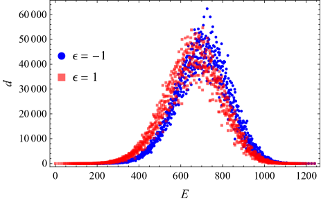
Figure 4: Energy $E$ vs. degeneracy $d$ of the spectrum of the $\mathrm{su}(1|2)$ HS chain of $BC_{N}$ type with $N=15$ spins and $\bar{\beta}=1$ for $\varepsilon=-1$ (blue circles) and $\varepsilon=1$ (pink squares).

7.2 $\mathrm{su}(1|1)$, arbitrary $N$

The partition function of the $\mathrm{su}(1|1)$ HS chain of $A_{N-1}$ type can be computed in closed form for arbitrary $N$, with the result CFGRT16

$$Z_{A,N}(q)=2\prod_{i=1}^{N-1}(1+q^{{\mathcal{E}}_{A}(i)})\,,$$

where we have explicitly indicated the dependence on $N$ for later convenience. A similar formula is in fact valid for the $A_{N-1}$ Polychronakos–Frahm Fr93 ; Po94 (rational) and Frahm–Inozemtsev FI94 (hyperbolic) chains, with ${\mathcal{E}}_{A}$ replaced by the dispersion relation of the latter chains. As in the $A_{N-1}$ case, the partition function of the $\mathrm{su}(1|1)$ HS chain of $BC_{N}$ type can be evaluated in closed form for arbitrary $N$, as we shall next show. In particular, we shall see that the result depends in an essential way on the two signs $\varepsilon$ and $\varepsilon^{\prime}$.

7.2.1 $\varepsilon=\varepsilon^{\prime}=1$

In this case $m_{\varepsilon}=n_{\varepsilon^{\prime}}=1$, and therefore $*=2$, $F=\{1\}$ and $B=\{2\}$. Since $2$ is bosonic, no type 1 tableaux of the form

$$\ytableausetup{nosmalltableaux}\overset{{}^{\hphantom{}\ytableaushort{\none\none}}{}^{\textstyle\iddots}}{\ytableaushort{\none{},\none{\raise-2.0pt\hbox{$\vdots$}},2{}}}$$

are allowed. Thus all allowed tableaux are of type 0, i.e., of the form

$$\overset{{}^{\hphantom{}\ytableaushort{\none}}{}^{\textstyle\iddots}}{\ytableaushort{{},{\raise-2.0pt\hbox{$\vdots$}},2}}$$

It is also clear that the $2$ in the last box imposes no additional restriction (apart from the standard rules for $(1|1)$ supersymmetric tableaux) on the box immediately on top of it. In other words, the number of tableaux of this form with $N+1$ boxes coincides with the number of regular $\mathrm{su}(1|1)$ tableaux with $N$ boxes obtained by removing the last (bottommost) box. We thus arrive at the formula

$$Z_{N}^{++}(q)=\sum_{\mathbf{k}\in{\mathcal{P}}_{N}}d_{A}(\mathbf{k})q^{\sum_{i=1}^{r-1}{\mathcal{E}}(K_{i})}\,.$$

Realizing that the RHS is nothing but $Z_{A,N}(q)$ with ${\mathcal{E}}_{A}$ replaced by ${\mathcal{E}}$ we conclude that

$$Z_{N}^{++}(q)=2\prod_{i=1}^{N-1}(1+q^{{\mathcal{E}}(i)})\,.$$

Thus the $\mathrm{su}(1|1)$ HS chain of $BC_{N}$ type with $\varepsilon=\varepsilon^{\prime}=1$ behaves essentially as a type $A_{N-1}$ chain with a different dispersion relation.

7.2.2 $\varepsilon=\varepsilon^{\prime}=-1$

We have $m_{\varepsilon}=n_{\varepsilon^{\prime}}=0$, and therefore $*=m_{\varepsilon}+n_{\varepsilon^{\prime}}=0$. Thus only type 1 tableaux are allowed, and it is again clear that the $0$ in the leftmost box entails no restriction (apart from the standard rules for $(1|1)$ supersymmetric tableaux) on the box to its right. We thus have

$$Z_{N}^{--}(q) =\sum_{\mathbf{k}\in{\mathcal{P}}_{N}}d_{A}(\mathbf{k})q^{{\mathcal{E}}(N)}q^{\sum_{i=1}^{r-1}{\mathcal{E}}(K_{i})}=q^{{\mathcal{E}}(N)}Z^{++}_{N}(q)$$

$$=2q^{{\mathcal{E}}(N)}\prod_{i=1}^{N-1}(1+q^{{\mathcal{E}}(i)})\,.$$

Thus the spectrum in this case is obtained by shifting the spectrum in the previous case by a constant (positive) energy ${\mathcal{E}}(N)$.

7.2.3 $\varepsilon=-\varepsilon^{\prime}=1$

In this case $m_{\varepsilon}=1$, $n_{\varepsilon^{\prime}}=0$, and hence $*=m_{\varepsilon}+n_{\varepsilon^{\prime}}=1$, $B=\{1\}$ and $F=\{2\}$. A moment’s reflection shows that all border strips $\langle k_{1},\dots,k_{r}\rangle$ give rise to exactly one allowed Young tableau, of the form

$$\ytableausetup{smalltableaux}\overset{{}^{\hphantom{}\ytableaushort{\none\none\none\none\none\none}}{}^{\textstyle\iddots}}{\ytableaushort{\none\none\none 12,\none\none\none{\raise-1.0pt\hbox{$\scriptscriptstyle\vdots$}},\none\none\none 1,12{\cdots}2,{\raise-1.0pt\hbox{$\scriptscriptstyle\vdots$}}\none,1\none,1\none}}\qquad\overset{{}^{\hphantom{}\ytableaushort{\none\none\none\none\none\none\none}}{}^{\textstyle\iddots}}{\ytableaushort{\none\none\none\none\none\none 1,\none\none\none 12\cdots 2,\none\none\none{\raise-1.0pt\hbox{$\scriptscriptstyle\vdots$}},\none\none\none 1,12\cdots 2}}$$

respectively for type 0 and 1 border strips. Thus the partition function is given in this case by

$$Z_{N}^{+-}(q) =\sum_{\mathbf{k}\in{\mathcal{P}}_{N+1}}q^{\sum_{i=1}^{r-1}{\mathcal{E}}(K_{i})}=1+\sum_{r=2}^{N}\,\sum_{1\leqslant K_{1}<\cdots<K_{r-1}\leqslant N}q^{\sum_{i=1}^{r-1}{\mathcal{E}}(K_{i})}$$

$$=\prod_{i=1}^{N}(1+q^{{\mathcal{E}}(i)}).$$

Thus the $\mathrm{su}(1|1)$ HS chain of $BC_{N}$ type with $\varepsilon=-\varepsilon^{\prime}=1$ is equivalent to a system of $N$ free spinless fermions with dispersion relation ${\mathcal{E}}$ (i.e., for which the energy of the single-particle mode with momentum $2k\pi/N$ is ${\mathcal{E}}(k)$).

7.2.4 $\varepsilon=-\varepsilon^{\prime}=-1$

Here $m_{\varepsilon}=0$, $n_{\varepsilon^{\prime}}=1$, and consequently $*=m_{\varepsilon}+n_{\varepsilon^{\prime}}=1$, $F=\{1\}$ and $B=\{2\}$. The difference with the previous case is that, even if now $1$ is of fermionic type, $*=1$ should be treated as a bosonic variable (cf. Remarks 4) and 5 above). As a consequence, type 0 and type 1 tableaux can only end in $\ytableaushort{1\cdots,1\none}$ and $\ytableaushort{\none\cdots,12}$, respectively, where in both cases $\ytableaushort{\cdots}$ stands for a standard $(1|1)$ supersymmetric tableaux with no additional restrictions. Since $K_{r-1}=N-1+\alpha$ for type $\alpha$ tableaux, we conclude that

$$Z_{N}^{-+}(q)=(q^{N-1}+q^{N})Z_{A,N-1}(q)\big{|}_{{\mathcal{E}}_{A}\to{\mathcal{E}}}=2\big{(}q^{{\mathcal{E}}(N-1)}+q^{{\mathcal{E}}(N)}\big{)}\prod_{i=1}^{N-2}(1+q^{{\mathcal{E}}(i)}).$$

7.2.5 Free energy

With the previous explicit formulas it is an easy matter to obtain an exact expression for the free energy per spin of the open $\mathrm{su}(1|1)$ HS chain (2.3) in the thermodynamic limit. To this end, we first normalize the Hamiltonian dividing it by $1/N^{2}$, in order to obtain a finite energy density in the thermodynamic limit. Since

$$\frac{{\mathcal{E}}(i)}{N^{2}}=x_{i}\bigg{(}1+\frac{\bar{\beta}}{N}-\frac{x_{i}}{2}-\frac{1}{2N}\bigg{)},\qquad x_{i}:=\frac{i}{N}\,\in(0,1],$$

we have

$$\frac{{\mathcal{E}}(i)}{N^{2}}\underset{N\to\infty}{\to}\frac{x}{2}\,(2\gamma-x)=:\varphi(x)\,,\qquad\gamma:=1+\lim_{N\to\infty}\frac{\bar{\beta}}{N}\geqslant 1\,,$$

where $x\in[0,1]$ is a continuous variable. The free energy per particle in the thermodynamic limit is then given in all four cases by

$$f(T)=-T\lim_{N\to\infty}\frac{1}{N}\log Z_{N}^{\varepsilon\varepsilon^{\prime}}\Bigl{(}\mathrm{e}^{-1/N^{2}T}\Bigr{)}=-T\int_{0}^{1}\log\bigl{(}1+\mathrm{e}^{-\varphi(x)/T}\bigr{)}\mathrm{d}x\,.$$

Changing to the momentum variable $p=\pi x$ we obtain

$$f(T)=-\frac{T}{\pi}\int_{0}^{\pi}\log\bigl{(}1+\mathrm{e}^{-\phi(p)/T}\bigr{)}\mathrm{d}p\,,$$ (7.1)

where the dispersion relation $\phi(p)$ is given by

$$\phi(p):=\varphi\Bigl{(}\tfrac{|p|}{\pi}\Bigr{)}=\frac{|p|}{2\pi^{2}}(2\pi\gamma-|p|)=\frac{1}{2\pi^{2}}\big{[}\pi^{2}\gamma^{2}-(|p|-\pi\gamma)^{2}\big{]}\,,\enspace\quad-\pi\leqslant p\leqslant\pi.$$ (7.2)

Figure 5: Dispersion relation $\phi(p)=|p|(2\pi\gamma-|p|)/2\pi^{2}$ of the $\mathrm{su}(1|1)$ supersymmetric HS chain of $BC_{N}$ type (2.3) in the thermodynamic limit for $\gamma>1$ (left) and $\gamma=1$ (right).

Thus in the thermodynamic limit all four variants of the $\mathrm{su}(1|1)$ HS chain of $BC_{N}$ type are equivalent to a system of free fermions with dispersion relation given by Eq. (7.2). The latter expression is of course reminiscent of the corresponding ones for the free energy per spin of the $A_{N-1}$-type HS, PF and FI chains obtained in Refs. CFGRT16 ; FGLR18 . It is clear that (when prolonged as a periodic function of period $2\pi$) $\phi(p)$ has a cusp at the points $p=k\pi$ with $k\in{\mathbb{Z}}$ when $\gamma>1$, or $2k\pi$ with $k\in{\mathbb{Z}}$ for $\gamma=1$ (cf. Fig. 5), much like what happens with the dispersion relation of the $A_{N-1}$-type PF and FI chains (when $\gamma>1$) or the HS chain (when $\gamma=1$). Since $\gamma\geqslant 1$, the dispersion relation is clearly monotonic in each of the intervals $[-\pi,0]$ and $[0,\pi]$, as is the case with the HS chains of $A_{N-1}$ type. Moreover, for $\gamma=1$ Eq. (7.2) coincides (up to a trivial rescaling by a factor of $1/\pi^{2}$) with the dispersion relation of the $\mathrm{su}(1|1)$ HS chain of $A_{N-1}$ type. This shows that the $\mathrm{su}(1|1)$ HS chain of $BC_{N}$ type with $\bar{\beta}/N\to 0$ as $N\to\infty$ is equivalent in the thermodynamic limit to its $A_{N-1}$ counterpart, a result that is far from obvious a priori.

8 Conclusions and outlook

The description of the spectrum of the Haldane–Shastry spin chain in terms of border strips (or, equivalently, motifs) and skew Young tableaux is one of the hallmarks in the theory of integrable spin chains with long-range interactions, underscoring the close connections of spin chains of HS type with the representation theory of Yangian algebras. In this paper we address the problem of finding a similar motif-based description of the spectrum of the open version of the (supersymmetric) Haldane–Shastry spin chain, associated with the $BC_{N}$ root system. More precisely, we first construct the model’s Hamiltonian by suitably extending the standard definition of the spin permutation and reversal operators to the supersymmetric case. We then compute its partition function in closed form by means of Polychronakos’s freezing trick, which basically consists in modding out the dynamical degrees of freedom of the associated $BC_{N}$-type spin Sutherland model. Inspired by the procedure for the closed ($A_{N-1}$) HS chain BBH10 , we construct a generalized partition function depending polynomially on two sets of vector variables, which reproduces the standard one when these variables are set equal to $1$. We then show that this generalized partition function can be expressed in terms of two variants of the standard skew super Schur polynomials, which can be defined through a simple combinatorial formula in terms of supersymmetric skew Young tableaux with an additional box filled with a fixed integer. With the help of this formula, we are able to derive a complete description of the spectrum of the supersymmetric HS chain of $BC_{N}$ type in terms of extended motifs and restricted Young tableaux, akin to the one for the closed HS chain. We illustrate this description with a few concrete examples, including a complete study of the $\mathrm{su}(1|1)$ model and its thermodynamics.

Much as in the $A_{N-1}$ case, the existence of a motif-based description of the spectrum of the model under study could prove of key importance for uncovering some of its fundamental properties. In the first place, such a description is a clear indication that the model possesses some kind of (twisted) Yangian symmetry. Obtaining an explicit realization of this symmetry, either via its generators or through a suitable monodromy matrix BPS95 , is certainly worth investigating. As in the $A_{N-1}$ case EFG12 ; FGLR18 , the motif-based description of the spectrum deduced in this work can be taken as the starting point for deriving its thermodynamics using the inhomogeneous transfer matrix approach. To this end, it is necessary to introduce a chemical potential term in the Hamiltonian and generalize the above results —in particular, the characterization of the spectrum in terms of restricted supersymmetric skew Young tableaux— to the model thus obtained. In fact, the detailed results for the $\mathrm{su}(1|1)$ chains derived in this paper strongly suggest that the thermodynamic functions in the general $\mathrm{su}(m|n)$ case can be obtained from those of the closed supersymmetric HS chain simply by replacing the dispersion relation of the latter model by that of the present one (cf. Eq. (3.13)). A related application of our results is the study of the model’s criticality by analyzing the low temperature asymptotic behavior of its Helmholtz free energy, which should exhibit the $T^{2}$ behavior characteristic of $(1+1)$-dimensional conformal field theories BCN86 ; Af86 at the critical phase.

(JC)

(MAR)

References

• (1) K. Kim, M.-S. Chang, R. Islam, S. Korenblit, L.-M. Duan and C. Monroe, Entanglement and tunable spin-spin couplings between trapped ions using multiple transverse modes, Phys. Rev. Lett. 103 (2009), 120502(4).
• (2) T. Graß and M. Lewenstein, Trapped-ion quantum simulation of tunable-range Heisenberg chains, EPJ Quantum Technology 1 (2014), 8(20).
• (3) P. Jurcevic, B. P. Lanyon, P. Hauke, C. Hempel, P. Zoller, R. Blatt and C. F. Roos, Quasiparticle engineering and entanglement propagation in a quantum many-body system, Nature 511 (2014), 202–205.
• (4) P. Richerme, Z.-X. Gong, A. Lee, C. Senko, J. Smith, M. Foss-Feig, S. Michalakis, A. V. Gorshkov and C. Monroe, Non-local propagation of correlations in quantum systems with long-range interactions, Nature 511 (2014), 198–201.
• (5) P. Schauß, J. Zeiher, T. Fukuhara, S. Hild, M. Chenau, T. Macrì, T. Pohl, I. Bloch and C. Gross, Crystallization in Ising quantum magnets, Science 347 (2015), 1455–1458.
• (6) C.-L. Hung, A. González-Tudela, J. I. Cirac and H. J. Kimble, Quantum spin dynamics with pairwise-tunable, long-range interactions, Proc. Natl. Acad. Sci. USA 113 (2016), E4946–E4955.
• (7) F. D. M. Haldane, Exact Jastrow–Gutzwiller resonating-valence-bond ground state of the spin-$1/2$ antiferromagnetic Heisenberg chain with $1/r^{2}$ exchange, Phys. Rev. Lett. 60 (1988), 635–638.
• (8) B. S. Shastry, Exact solution of an ${S}=1/2$ Heisenberg antiferromagnetic chain with long-ranged interactions, Phys. Rev. Lett. 60 (1988), 639–642.
• (9) F. D. M. Haldane, “Spinon gas” description of the ${S}=\frac{1}{2}$ Heisenberg chain with inverse-square exchange: exact spectrum and thermodynamics, Phys. Rev. Lett. 66 (1991), 1529–1532.
• (10) F. D. M. Haldane, Physics of the ideal semion gas: spinons and quantum symmetries of the integrable Haldane–Shastry spin chain, in A. Okiji and N. Kawakami, eds., Correlation Effects in Low-dimensional Electron Systems, vol. 118 of Springer Series in Solid-state Sciences (1994), pp. 3–20.
• (11) F. D. M. Haldane, “Fractional statistics” in arbitrary dimensions: a generalization of the Pauli principle, Phys. Rev. Lett. 67 (1991), 937–940.
• (12) H. Azuma and S. Iso, Explicit relation of the quantum Hall effect and the Calogero–Sutherland model, Phys. Lett. B 331 (1994), 107–113.
• (13) E. J. Bergholtz and A. Karlhede, Quantum Hall circle, J. Stat. Mech.-Theory E. 2014 (2014), P04015(12).
• (14) C. W. J. Beenakker and B. Rajaei, Exact solution for the distribution of transmission eigenvalues in a disordered wire and comparison with random-matrix theory, Phys. Rev. B 49 (1994), 7499–7510.
• (15) M. Caselle, Distribution of transmission eigenvalues in disordered wires, Phys. Rev. Lett. 74 (1995), 2776–2779.
• (16) J. I. Cirac and G. Sierra, Infinite matrix product states, conformal field theory, and the Haldane–Shastry model, Phys. Rev. B 81 (2010), 104431(4).
• (17) A. E. B. Nielsen, J. I. Cirac and G. Sierra, Quantum spin Hamiltonians for the $su(2)_{k}$ WZW model, J. Stat. Mech.-Theory E. 2011 (2011), P11014(39).
• (18) R. Bondesan and T. Quella, Infinite matrix product states for long-range SU$(N)$ spin models, Nucl. Phys. B 886 (2014), 483–523.
• (19) H.-H. Tu, A. E. B. Nielsen and G. Sierra, Quantum spin models for the $\mathrm{SU}(n)_{1}$ Wess–Zumino–Witten model, Nucl. Phys. B 886 (2014), 328–363.
• (20) B. Sutherland, Exact results for a quantum many-body problem in one dimension. II, Phys. Rev. A 5 (1972), 1372–1376.
• (21) Z. N. C. Ha and F. D. M. Haldane, Models with inverse-square exchange, Phys. Rev. B 46 (1992), 9359–9368.
• (22) A. P. Polychronakos, Lattice integrable systems of Haldane–Shastry type, Phys. Rev. Lett. 70 (1993), 2329–2331.
• (23) A. P. Polychronakos, Exact spectrum of $\mathrm{SU}(n)$ spin chain with inverse-square exchange, Nucl. Phys. B 419 (1994), 553–566.
• (24) F. Finkel and A. González-López, Global properties of the spectrum of the Haldane–Shastry spin chain, Phys. Rev. B 72 (2005), 174411(6).
• (25) J. C. Barba, F. Finkel, A. González-López and M. A. Rodríguez, The Berry–Tabor conjecture for spin chains of Haldane–Shastry type, Europhys. Lett. 83 (2008), 27005(6).
• (26) H. Frahm and V. I. Inozemtsev, New family of solvable 1D Heisenberg models, J. Phys. A: Math. Gen. 27 (1994), L801–L807.
• (27) J. C. Barba, F. Finkel, A. González-López and M. A. Rodríguez, Inozemtsev’s hyperbolic spin model and its related spin chain, Nucl. Phys. B 839 (2010), 499–525.
• (28) F. Calogero, Solution of the one-dimensional ${N}$-body problems with quadratic and/or inversely quadratic pair potentials, J. Math. Phys. 12 (1971), 419–436.
• (29) J. A. Minahan and A. P. Polychronakos, Integrable systems for particles with internal degrees of freedom, Phys. Lett. B 302 (1993), 265–270.
• (30) V. I. Inozemtsev, Exactly solvable model of interacting electrons confined by the Morse potential, Phys. Scr. 53 (1996), 516–520.
• (31) B. Basu-Mallick and N. Bondyopadhaya, Exact partition functions of $\mathrm{SU}(m|n)$ supersymmetric Haldane–Shastry spin chain, Nucl. Phys. B 757 (2006), 280–302.
• (32) B. Basu-Mallick, H. Ujino and M. Wadati, Exact spectrum and partition function of $\mathrm{SU}(m|n)$ supersymmetric Polychronakos model, J. Phys. Soc. Jpn. 68 (1999), 3219–3226.
• (33) B. Basu-Mallick and N. Bondyopadhaya, Spectral properties of supersymmetric Polychronakos spin chain associated with $A_{N-1}$ root system, Phys. Lett. A 373 (2009), 2831–2836.
• (34) F. D. M. Haldane, Z. N. C. Ha, J. C. Talstra, D. Bernard and V. Pasquier, Yangian symmetry of integrable quantum chains with long-range interactions and a new description of states in conformal field theory, Phys. Rev. Lett. 69 (1992), 2021–2025.
• (35) D. Bernard, M. Gaudin, F. D. M. Haldane and V. Pasquier, Yang–Baxter equation in long-range interacting systems, J. Phys. A: Math. Gen. 26 (1993), 5219–5236.
• (36) A. N. Kirillov, A. Kuniba and T. Nakanishi, Skew Young diagram method in spectral decomposition of integrable lattice models, Commun. Math. Phys. 185 (1997), 441–465.
• (37) M. Nazarov and V. Tarasov, Representations of Yangians with Gelfand–Zetlin bases, J. Reine Angew. Math 496 (1998), 181–212.
• (38) B. Basu-Mallick, N. Bondyopadhaya, K. Hikami and D. Sen, Boson-fermion duality in $\mathrm{SU}(m|n)$ supersymmetric Haldane–Shastry spin chain, Nucl. Phys. B 782 (2007), 276–295.
• (39) B. Basu-Mallick, N. Bondyopadhaya and K. Hikami, One-dimensional vertex models associated with a class of Yangian invariant Haldane–Shastry like spin chains, Symmetry Integr. Geom. 6 (2010), 091(13).
• (40) K. Hikami and B. Basu-Mallick, Supersymmetric Polychronakos spin chain: motif, distribution function, and character, Nucl. Phys. B 566 (2000), 511–528.
• (41) A. Enciso, F. Finkel and A. González-López, Thermodynamics of spin chains of Haldane–Shastry type and one-dimensional vertex models, Ann. Phys.-New York 327 (2012), 2627–2665.
• (42) F. Finkel, A. González-López, I. León and M. A. Rodríguez, Thermodynamics and criticality of supersymmetric spin chains with long-range interactions, J. Stat. Mech.-Theory E. 2018 (2018), 043101(47).
• (43) M. A. Olshanetsky and A. M. Perelomov, Quantum integrable systems related to Lie algebras, Phys. Rep. 94 (1983), 313–404.
• (44) D. Bernard, V. Pasquier and D. Serban, Exact solution of long-range interacting spin chains with boundaries, Europhys. Lett. 30 (1995), 301–306.
• (45) T. Yamamoto, Multicomponent Calogero model of ${B}_{N}$-type confined in a harmonic potential, Phys. Lett. A 208 (1995), 293–302.
• (46) F. Finkel, D. Gómez-Ullate, A. González-López, M. A. Rodríguez and R. Zhdanov, On the Sutherland model of ${B}_{{N}}$ type and its associated spin chain, Commun. Math. Phys. 233 (2003), 191–209.
• (47) A. Enciso, F. Finkel, A. González-López and M. A. Rodríguez, Haldane–Shastry spin chains of $BC_{N}$ type, Nucl. Phys. B 707 (2005), 553–576.
• (48) J. C. Barba, F. Finkel, A. González-López and M. A. Rodríguez, An exactly solvable supersymmetric spin chain of $BC_{N}$ type, Nucl. Phys. B 806 (2009), 684–714.
• (49) B. Basu-Mallick, F. Finkel and A. González-López, Exactly solvable $D_{N}$-type quantum spin models with long-range interaction, Nucl. Phys. B 812 (2009), 402–423.
• (50) B. Basu-Mallick, F. Finkel and A. González-López, The spin Sutherland model of $D_{N}$ type and its associated spin chain, Nucl. Phys. B 843 (2011), 505–553.
• (51) B. Basu-Mallick, F. Finkel and A. González-López, The exactly solvable spin Sutherland model of $B_{N}$ type and its related spin chain, Nucl. Phys. B 866 (2013), 391–413.
• (52) H.-H. Tu and G. Sierra, Infinite matrix product states, boundary conformal field theory, and the open Haldane–Shastry model, Phys. Rev. B 92 (2015), 041119(R5).
• (53) B. Basu-Mallick, F. Finkel and A. González-López, Integrable open spin chains related to infinite matrix product states, Phys. Rev. B 155154(10) (2016), 391–413.
• (54) B. Basu-Mallick and M. Sinha, Appearance of branched motifs in the spectra of $BC_{N}$ type Polychronakos spin chains, Nucl. Phys. B 952 (2020), 114914(37).
• (55) B. Basu-Mallick and C. Datta, Super Rogers–Szegö polynomials associated with $BC_{N}$ type of Polychronakos spin chains, Nucl. Phys. B 921 (2017), 59–85.
• (56) F. Finkel and A. González-López, Yangian-invariant spin models and Fibonacci numbers, Ann. Phys.-New York 361 (2015), 520–547.
• (57) E. Corrigan and R. Sasaki, Quantum versus classical integrability in Calogero–Moser systems, J. Phys. A: Math. Gen. 35 (2002), 7017–7061.
• (58) S. Odake and R. Sasaki, Polynomials associated with equilibrium positions in Calogero–Moser systems, J. Phys. A: Math. Gen. 35 (2002), 8283–8314.
• (59) I. G. Macdonald, Symmetric Functions and Hall Polynomials, 2nd edn., Oxford University Press, Oxford (1995).
• (60) J. A. Carrasco, F. Finkel, A. González-López, M. A. Rodríguez and P. Tempesta, Critical behavior of $\mathrm{su}(1|1)$ supersymmetric spin chains with long-range interactions, Phys. Rev. E 93 (2016), 062103(12).
• (61) H. Frahm, Spectrum of a spin chain with inverse-square exchange, J. Phys. A: Math. Gen. 26 (1993), L473–L479.
• (62) H. W. J. Blöte, J. L. Cardy and M. P. Nightingale, Conformal invariance, the central charge, and universal finite-size amplitu des at criticality, Phys. Rev. Lett. 56 (1986), 742–745.
• (63) I. Affleck, Universal term in the free energy at a critical point and the conformal anomaly, Phys. Rev. Lett. 56 (1986), 746–748.
(JC)
(MAR)