Toward Evaluating Re-identification Risks in the Local Privacy Model

Abstract

LDP (Local Differential Privacy) has recently attracted much attention as a metric of data privacy that prevents the inference of personal data from obfuscated data in the local model. However, there are scenarios in which the adversary wants to perform re-identification attacks to link the obfuscated data to users in this model. LDP can cause excessive obfuscation and destroy the utility in these scenarios because it is not designed to directly prevent re-identification. In this paper, we propose a measure of re-identification risks, which we call PIE (Personal Information Entropy). The PIE is designed so that it directly prevents re-identification attacks in the local model. It lower-bounds the lowest possible re-identification error probability (i.e., Bayes error probability) of the adversary. We analyze the relation between LDP and the PIE, and analyze the PIE and utility in distribution estimation for two obfuscation mechanisms providing LDP. Through experiments, we show that when we consider re-identification as a privacy risk, LDP can cause excessive obfuscation and destroy the utility. Then we show that the PIE can be used to guarantee low re-identification risks for the local obfuscation mechanisms while keeping high utility.

1 Introduction

With the widespread use of personal computers, mobile devices, and IoT (Internet-of-Things) devices, a great amount of personal data (e.g., location data [91], rating history data [1], browser settings [31]) are increasingly collected and used for data analysis. However, the collection of personal data can raise serious privacy concerns. For example, users’ sensitive locations (e.g., hospitals, stores) can be estimated from their location traces (time-series location trails). Even if location traces are pseudonymized, they can be re-identified (de-anonymized) to link location traces with user IDs [37, 56, 57]. An anonymized rating dataset can also be de-anonymized to learn sensitive ratings of users [60].

DP (Differential Privacy) [27, 28] is a privacy metric that protects users’ privacy against adversaries with arbitrary background knowledge, and is known as a gold standard for data privacy. According to the underlying architecture, DP can be divided into the centralized DP and LDP (Local DP). The centralized DP assumes a centralized model, in which a trusted data collector, who has access to all user’s personal data, obfuscates the data. On the other hand, LDP assumes a local model, in which a user obfuscates her personal data by herself and sends the obfuscated data to a (possibly malicious or untrustworthy) data collector. While all user’s personal data can be leaked from the data collector by illegal access in the centralized model, LDP does not suffer from such data leakage. Thus LDP has been recently studied in the literature [7, 19, 34, 45, 58, 63, 86] and has been adopted by several industrial applications [31, 24, 77].

However, LDP is designed as a metric of data privacy that aims to prevent the inference of personal data (i.e., guarantee the indistinguishability of the original data), and there are scenarios in which we should consider user privacy that aims to prevent re-identification in the local model. Below we present two examples of the scenarios.

The first example is an application that does not require user IDs. The main application of LDP is estimating aggregate statistics such as a distribution of personal data [34, 45, 58, 86] and heavy hitters [7, 86]. In this case, what are needed are each user’s obfuscated data (e.g., noisy locations, noisy purchase history), and her user ID does not have to be collected. In fact, some applications (e.g., Google Maps, Foursquare, YouTube recommendations) can be used without requiring a user login. In such applications, the adversary (who can be either the data collector or outsider) obtains only the obfuscated data, and wants to perform a re-identification attack to identify the user who has sent the obfuscated data.

The second example is pseudonymization. Suppose a mobile application which sends both the user ID and personal (or obfuscated) data to the data collector. The data collector can pseudonymize all personal (or obfuscated) data to reduce the risks to the users, as described in GDPR [78]. In this case, an outsider adversary who obtains the personal (or obfuscated) data via illegal access has to re-identify the user. Despite the importance of re-identification risks in the local model, a metric of re-identification risks in this model has not been well established (see Section 2 for details).

One might think that LDP with a small privacy budget $\varepsilon$ (e.g., $\varepsilon\leq 1$ [51]) is enough to prevent re-identification attacks because it guarantees the indistinguishability of the original personal data. In other words, if personal data are obfuscated so that the adversary cannot infer the original data, then it seems to be impossible for the adversary to re-identify the user. This is indeed the case – we also show that LDP with a small privacy budget $\varepsilon$ prevents re-identificatiion in our experiments. However, the real issue of LDP is that it is not designed to directly prevent re-identification, and it makes the original data indistinguishable from any other possible data in the data domain. This can cause excessive obfuscation and destroy the utility, as shown in this paper.

Our Contributions.  In this paper, we make the following contributions:

1) PIE (Personal Information Entropy).  We propose a measure of re-identification risks in the local model, which we call the PIE (Personal Information Entropy). The PIE is given by the mutual information between a user and (possibly obfuscated) personal data. The PIE is applicable to any kind of personal data, and does not specify an identification algorithm used by an adversary. The PIE lower-bounds the lowest possible re-identification error probability (i.e., Bayes error probability) of the adversary. We also propose a privacy metric called PIE privacy that upper-bounds the PIE irrespective of the adversary’s background knowledge. We also show that pseudonymization (random permutation) alone guarantees a high re-identification error probability in some cases using our PIE, whereas random permutation alone cannot guarantee DP even using its average versions (e.g., Kullback-Leibler DP [6, 21], mutual information DP [21]) or recently proposed shuffling techniques [5, 30].

2) Theoretical Analysis of the PIE for Obfuscation Mechanisms.  We analyze the PIE for two existing local obfuscation mechanisms: the RR (Randomized Response) for multiple alphabets [45] and the generalized version of local hashing in [86], which we call the GLH (General Local Hashing). Both of them are mechanisms providing LDP, and can be used to examine the relationship between LDP and the PIE.

We first show that our PIE privacy is a relaxation of LDP; i.e., any LDP mechanism provides PIE privacy, hence upper-bounds the PIE. Then we show that this general upper-bound on the PIE for any LDP mechanism is loose, and show much tighter upper-bounds on the PIE for the RR and GLH.

3) Theoretical Analysis of the Utility for Obfuscation Mechanisms.  We analyze the utility of the RR and GLH for given PIE guarantees. Here, we consider discrete distribution estimation [2, 3, 34, 45, 46, 58], where personal data take discrete values, as a task for the data collector.

In our utility analysis, we show that our PIE privacy has a very different implication for utility and privacy than LDP. Specifically, let $\mathcal{X}$ be a finite set of personal data. Then the GLH reduces the size $|\mathcal{X}|$ of personal data to $g$ (i.e., dimension reduction) via random projection. When we use LDP as a privacy metric, the optimal value of $g$ is given by: $g=e^{\varepsilon}+1$ [86], where $\varepsilon$ is a privacy budget of LDP. In contrast, we show that when we use PIE privacy as a privacy metric, a larger $g$ provides better utility. In other words, we show an intuitive result that compressing the personal data with a smaller $g$ results in the loss of utility in our privacy metric. This result is caused by the fact that PIE privacy prevents the identification of users, whereas LDP prevents the inference of personal data.

4) Evaluating the PIE for Obfuscation Mechanisms.  We evaluate the privacy and utility the RR and GLH. We first show that LDP destroys utility when the privacy budget $\varepsilon$ is small. For example, for distribution estimation of the most popular $20$ POIs (Point-of-Interests) in the Foursquare dataset [89], the relative error of the RR was $1.05$ $(>1)$ even when $\varepsilon=10$ (which is considered to be still fairly large [51]). In other words, LDP fails to guarantee meaningful privacy and utility for this task. This comes from the fact that LDP is not designed to directly prevent re-identification attacks.

We next show that the PIE can be used to guarantee a low re-identification error while keeping high utility. For example, when we used the PIE to guarantee the re-identification error probability larger than $0.92$, the relative error of the RR for the top-$20$ POIs was $0.10$ $(\ll 1)$. This suggests that when we consider re-identification as a privacy risk, we should design a privacy metric that directly prevents re-identification attacks.

5) PSE (Personal Identification System Entropy).  As explained above, we show upper-bounds on the PIE for the RR and GLH. Then a natural question would be “how tight are these upper-bounds?” To answer to this question, we introduce the PSE (Personal Identification System Entropy), which is a lower-bound on the PIE and is equal to the PIE under some conditions. The PSE is designed to be easily calculated by specifying an identification algorithm. We show through experiments that our upper-bounds on the PIE for the RR and GLH are close to the PSE, which indicates that our upper-bounds are fairly tight and cannot be improved much.

One additional interesting feature of the PSE is that it can be used to compare the identifiability of personal data such as location traces and rating history with the identifiability of biometric data such as a fingerprint and face. Nowadays biometric authentication is widely used for various applications such as unlocking a smartphone, banking, and physical access control. Our PSE provides a new intuitive understanding of re-identification risks by comparing two different sources of information.

Note that we do not consider privacy risks or obfuscation (e.g., adding DP noise) for biometric data. Our interest here is intuitive understanding of the identifiability of personal data (e.g., locations, rating history) through the comparison with biometric data.

For example, we show that a location trace with at least $500$ locations has higher identifiability than the face matcher in [61]. We also note that the face dataset in [61] has lower errors than the best matcher in the FRPC (Face Recognition Prize Challenge) 2017 [39] where face images were collected without tight quality constraints. In other words, we reveal the fact that the location trace is more identifiable than the face matcher that won the 1st place in the FRPC 2017. We believe that this result is of independent interest.

Remark.  Our PIE privacy is based on the mutual information, which quantifies the average amount of information about a user through observing (possibly obfuscated) personal data. Thus our PIE privacy is an average privacy notion, as with the KL (Kullback-Leibler)-DP [6, 21] and the mutual information DP [21]. Average privacy notions have also been used in some studies on location privacy [65, 69, 71].

The caveat of the average privacy notion is that it may not guarantee the indistinguishability for every user; e.g., even if it guarantees the re-identification error probability larger than $0.99$, at most $1\%$ of users may be re-identified. Nevertheless, there are application scenarios in which the average privacy notion is quite useful in practice. One example is a prioritization system that determines, among several defenses, which one should be (or should not be) used. Another example is an alerting system adopted in [18], which notifies engineers if re-identification risks exceed pre-determined limits. Thus, we use the average privacy notion as a starting point.

We also note that a worst-case privacy notion (e.g., min-entropy [72]) can be used to guarantee stronger privacy for every user. We leave extending our PIE privacy to the worst-case notion for future work (Section 6 describes some open questions in this research direction).

Basic Notations.  Let $\mathbb{N}$, $\mathbb{R}$, and $\mathbb{R}_{\geq 0}$ be the set of natural numbers, real numbers, and non-negative real numbers, respectively. For $a\in\mathbb{N}$, let $[a]=\{1,2,\cdots,a\}$. For random variables $A$ and $B$, let $I(A;B)$ be the mutual information between $A$ and $B$. For two distributions $p$ and $q$, let $D(p||q)$ be the KL (Kullback-Leibler) divergence [20]. We simply denote the logarithm with base 2 by $\log$. We use these notations throughout this paper.

2 Related Work

In this section, we review the previous work. Section 2.1 describes LDP [26] and other privacy metrics. Section 2.2 explains the RR for multiple alphabets [45] and the GLH [7].

2.1 Privacy Metrics

LDP.  Let $\mathcal{X}$ be a finite set of personal data, and $\mathcal{Y}$ be a finite set of obfuscated data. Let $\mathbf{Q}$ be an obfuscation mechanism (a.k.a. masking method [80]), which maps personal data $x\in\mathcal{X}$ to obfuscated data $y\in\mathcal{Y}$ with probability $\mathbf{Q}(y|x)$. Then LDP is defined as follows:

Definition 2.1 ($\varepsilon$-LDP).

Let $\varepsilon\in\mathbb{R}_{\geq 0}$. An obfuscation mechanism $\mathbf{Q}$ provides $\varepsilon$-LDP if for any $x,x^{\prime}\in\mathcal{X}$ and any $y\in\mathcal{Y}$,

$$\mathbf{Q}(y|x)\leq e^{\varepsilon}\mathbf{Q}(y|x^{\prime}).$$ (1)

Intuitively, LDP guarantees that the adversary who obtains $y$ cannot determine whether it comes from $x$ or $x^{\prime}$ for any pair of $x$ and $x^{\prime}$ in $\mathcal{X}$ with a certain degree of confidence. The parameter $\varepsilon$ is called the privacy budget. When the privacy budget $\varepsilon$ is close to $0$, all of the data in $\mathcal{X}$ are almost equally likely. Thus LDP strongly protects $y$ when $\varepsilon$ is small; e.g., $\varepsilon\leq 1$ [51].

Other Privacy Metrics.  To date, numerous variants of DP (or LDP) have been proposed to provide different types of privacy guarantees. Examples are: Pufferfish privacy [48], $d_{x}$-privacy [16], Rényi DP [54], concentrated DP [29], mutual information DP [21], personalized DP [44], utility-optimized LDP [58], and capacity-bounded DP [17]. A recent SoK paper proposed a systematic taxonomy of relaxations of DP, and classified the relaxations into seven categories based on which aspect of DP was modified [23].

Our PIE privacy is also a variant of DP because it is a relaxation of LDP, as shown in Sections 4.1. Our PIE privacy differs from existing variants of DP in that PIE privacy aims at preventing re-identification attacks. In this regard, PIE privacy is different from any dimension of seven categories in the SoK paper [23].

Our PIE and PSE are also related to quantitative information flow [4, 10, 65, 72], where the amount of information leakage is measured by the mutual information or entropy. In particular, our PSE is closely related to a recent study [65], which uses the mutual information between a user ID and a re-identified user ID as a measure of re-identification risks.

Our PSE differs from [65] in that the PSE is given by the mutual information between a user ID and a score vector (vector consisting of similarities or distances for all users) calculated by the adversary, rather than the re-identified user ID. We use the score vector because it contains much richer information than the identified user ID (this is well known in biometrics; e.g., see [66]). We also show that although the PSE is upper-bounded by the PIE, the PSE is equal to the PIE under some conditions (Section 3.2). This property is very useful for evaluating how tight an upper-bound on the PIE is. In fact, we show that our upper-bounds on the PIE for the RR and GLH are close to the PSE in our experiments (Section 5). In contrast, it is difficult to evaluate the upper-bounds on the PIE using the re-identification user ID because it contains much less information. We also note that a score vector enables us to output a list of $k\in[n]$ users whose similarities (resp. distance) are the highest (resp. lowest) as an identification result.

2.2 Obfuscation Mechanisms

RR for Multiple Alphabets.  The RR (Randomized Response) was originally introduced by Warner for binary alphabets [87]. Kairouz et al. [45] studied the RR for $|\mathcal{X}|$-ary alphabets.

Given $\varepsilon\in\mathbb{R}_{\geq 0}$, let $\mathbf{Q}_{RR}$ be the $\varepsilon$-RR for $|\mathcal{X}|$-ary alphabets. In the $\varepsilon$-RR, the output range is identical to the input domain; i.e., $|\mathcal{X}|=|\mathcal{Y}|$. Given personal data $x\in\mathcal{X}$, the $\varepsilon$-RR outputs obfuscated data $y\in\mathcal{X}$ with probability:

$$\mathbf{Q}_{\it RR}(y|x)=\begin{cases}\frac{e^{\varepsilon}}{|\mathcal{X}|+e^{\varepsilon}-1}&\text{(if $y=x$)}\\ \frac{1}{|\mathcal{X}|+e^{\varepsilon}-1}&\text{(otherwise)}.\\ \end{cases}$$ (2)

By (1) and (2), the $\varepsilon$-RR provides $\varepsilon$-LDP.

Note that the $\varepsilon$-RR is a kind of PRAM (Post-RAndomization Method) [80, 76, 53], which replace a category $x\in\mathcal{X}$ with another category $y\in\mathcal{X}$ according to a given transition matrix ($\mathbf{Q}$ can be viewed as a transition matrix), and that there is a connection between the literature of DP and that of PRAM. For example, Marés and Shlomo [53] consider a PRAM transition matrix whose diagonal values do not exceed $0.75$ to reduce privacy disclosure risks. When $\varepsilon=1$ (which is considered to be acceptable in the literature of DP [51]) in the $\varepsilon$-RR, the diagonal values in $\mathbf{Q}_{\it RR}$ are smaller than $0.73$ for any $|\mathcal{X}|\geq 2$ (by (2)).

GLH.  Bassily and Smith [7] proposed an obfuscation mechanism based on random projection that maps personal data $x\in\mathcal{X}$ to a single bit. Wang et al. [86] called this mechanism the BLH (Binary Local Hashing), and generalized it so that $x\in\mathcal{X}$ is mapped to a value in $[g]$, where $g\in\mathbb{N}$. We call this generalized mechanism the GLH (General Local Hashing).

The GLH consists of the following two steps: (i) apply random projection to $x\in\mathcal{X}$, and then (ii) perturb the data using the RR for multiple alphabets. Formally, let $\mathcal{H}=\{h:\mathcal{X}\rightarrow[g]\}$ be a universal hash function family [13]; i.e., for any distinct $x$ and $x^{\prime}$ in $\mathcal{X}$ and a hash function $h$ chosen uniformly at random in $\mathcal{H}$,

$$\Pr[h(x)=h(x^{\prime})]\leq\frac{1}{g}.$$

Given $\varepsilon\in\mathbb{R}_{\geq 0}$, let $\mathbf{Q}_{\it GLH}$ be the $(g,\varepsilon)$-GLH. The $(g,\varepsilon)$-GLH is an obfuscation mechanism with the input alphabet $\mathcal{X}$ and the output alphabets $\mathcal{Y}=(\mathcal{H},[g])$. Given $x\in\mathcal{X}$, the $(g,\varepsilon)$-GLH randomly generates a hash function $h$ from $\mathcal{H}$, and outputs $(h,y)\in\mathcal{Y}$ with probability:

$$\mathbf{Q}_{\it GLH}((h,y)|x)=\begin{cases}\frac{e^{\varepsilon}}{g+e^{\varepsilon}-1}&\text{(if $y=h(x)$)}\\ \frac{1}{g+e^{\varepsilon}-1}&\text{(otherwise)}.\\ \end{cases}$$ (3)

By (1) and (3), the $(g,\varepsilon)$-GLH provides $\varepsilon$-LDP. Wang et al. [86] found that for a fixed $\varepsilon$, the value of $g$ that minimizes the variance in distribution estimation is given by: $g=e^{\varepsilon}+1$.

3 Personal Information Entropy

We propose the PIE (Personal Information Entropy) as a measure of re-identification risks in the local model. We first describe frameworks for obfuscation and identification assumed in our work in Section 3.1. Then in Section 3.2, we introduce the PIE and a privacy metric called PIE privacy, which upper-bounds the PIE. We also introduce the PSE (Personal Identification System Entropy), which lower-bounds the PIE by specifying an identification algorithm. Finally we show several basic properties of the PIE in Section 3.3.

3.1 Obfuscation/Identification Framework

Framework.  Figures 2 and 2 show an obfuscation framework and identification framework, respectively. We also show in Table 1 the notations used in this paper. Let $\Omega$ be a finite set of all human beings, and $\mathcal{U}\subseteq\Omega$ be a finite set of users who use a certain application; e.g., location-based service, recommendation service. Let $n\in\mathbb{N}$ be the number of users in $\mathcal{U}$, and $u_{i}\in\mathcal{U}$ be the $i$-th user; i.e., $\mathcal{U}=\{u_{1},\cdots,u_{n}\}$.

Figure 1: Framework for obfuscation. Our PIE is built upon this obfuscation framework. The PIE does not specify any identification algorithm.

Figure 2: Framework for identification. A score vector $\mathbf{s}=(s_{1},\cdots,\allowbreak s_{n})\in\mathbb{R}^{n}$ consists of a numerical score (similarity or distance) $s_{i}\in\mathbb{R}$ between obfuscated data $Y$ and auxiliary information $r_{i}$ of user $u_{i}$. Our PSE is built upon this identification framework.

Table 1: Notations in this paper.

Symbol Description $\mathcal{U}$ Finite set of users. $\mathcal{X}$ Finite set of personal data. $\mathcal{Y}$ Finite set of obfuscated data. $\mathcal{R}$ Finite set of auxiliary data. $n$ Number of users in $\mathcal{U}$ ($n\in\mathbb{N}$). $u_{i}$ $i$-th user ($u_{i}\in\mathcal{U}$). $r_{i}$ Auxiliary information of user $u_{i}$. $s_{i}$ Score of user $u_{i}$ ($s_{i}\in\mathbb{R}$). $\mathbf{s}$ Score vector ($\mathbf{s}=(s_{1},\cdots,\allowbreak s_{n})\in\mathbb{R}^{n}$). $U$ Random variable representing a user in $\mathcal{U}$. $X$ Random variable representing personal data. $Y$ Random variable representing obfuscated data. $\mathbf{S}$ Random variable representing a score vector. $p_{U}$ Distribution of $U$. $p_{X|U=u_{i}}$ Distribution of $X$ given $U=u_{i}$. $p_{U,X}$ Joint distribution of $U$ and $X$. $\mathbf{Q}$ Obfuscation mechanism. $\mathcal{F}$ Matching algorithm. $\mathcal{G}$ Decision algorithm.

In the obfuscation phase, a user obfuscates her personal data by herself using an obfuscation mechanism $\mathbf{Q}$ in her device, and sends the obfuscated data to a data collector. Let $U$, $X$, and $Y$ be random variables representing a user in $\mathcal{U}$, personal data in $\mathcal{X}$, and obfuscated data in $\mathcal{Y}$, respectively.

User $U$ is randomly generated from some distribution over $\mathcal{U}$, which can be either uniform or non-uniform. Let $p_{U}$ be a distribution of $U$; i.e., $p_{U}(u_{i})=\Pr(U=u_{i})$. Note that $p_{U}$ is a prior distribution an adversary has before observing $Y$. In other words, $p_{U}$ is a kind of the adversary’s background knowledge. For example, suppose that each user sends a single obfuscated datum to a data collector, and that Alice’s obfuscated data $Y$ is leaked to the adversary. In this case, the prior distribution $p_{U}$ for this adversary is uniform over $\mathcal{U}$; i.e., $p_{U}(u_{i})=\frac{1}{|\mathcal{U}|}$ for any $u_{i}\in\mathcal{U}$. If some heavy users send obfuscated data many times and the adversary knows this fact, then $U$ is non-uniformly distributed.

Given $U=u_{i}$, personal data $X$ is randomly generated from some distribution over $\mathcal{X}$. Let $p_{X|U=u_{i}}$ be a distribution of $X$ given $U=u_{i}$; i.e., $p_{X|U=u_{i}}(x)=\Pr(X=x|U=u_{i})$. If personal data $X$ is uniquely determined given user $u_{i}$ (i.e., 4-digit PIN of Alice is “3928”), then $p_{X|U=u_{i}}$ is a point distribution that has probability $1$ for a single data point. Otherwise (e.g., Alice may visit many locations), $p_{X|U=u_{i}}$ is not a point distribution.

Let $p_{U,X}$ be a joint distribution of $U$ and $X$; i.e., $p_{U,X}(u_{i},x)=\Pr(U=u_{i},X=x)$. Note that $p_{U,X}(u_{i},x)=p_{U}(u_{i})p_{X|U=u_{i}}(x)$. As with $p_{U}$, $p_{U,X}$ is also a kind of the adversary’s background knowledge. Our PIE depends on $p_{U,X}$, but our PIE privacy does not depend on $p_{U,X}$, as described in Section 3.2 in detail.

Given $X=x$, obfuscated data $Y$ is randomly generated using an obfuscation mechanism $\mathbf{Q}$, which maps $x$ to $y\in\mathcal{Y}$ with probability $\mathbf{Q}(y|x)$. Examples of $\mathbf{Q}$ include the randomized response [87, 45], GLH [86], and RAPPOR [31]. If an obfuscation mechanism $\mathbf{Q}$ is not used, then $Y=X$. Then the data collector estimates some aggregate statistics; e.g., histogram, heavy hitters.

Our PIE is built upon the obfuscation framework in Figure 2, and is given by the mutual information between $U$ and $Y$, as described in Section 3.2. Therefore, the PIE does not specify any identification algorithm.

On the other hand, our PSE is designed to evaluate a lower-bound on the PIE through experiments by specifying an identification algorithm. The PSE is built upon the identification framework in Figure 2, where an identification system comprises two algorithms: a matching algorithm and decision algorithm. These algorithms are widely used for re-identification attacks in privacy literature [35, 37, 56, 57, 60, 69, 70].

In the identification phase, the matching algorithm takes as input obfuscated data $Y$ and some auxiliary information of user $u_{i}$, and outputs a numerical score for $u_{i}$. The auxiliary information is background knowledge about user $u_{i}$ the system possesses. The score is either a similarity or distance between the obfuscated data $Y$ and auxiliary information of $u_{i}$. A large similarity (or small distance) indicates that it is highly likely that $Y$ belongs to $u_{i}$.

For the auxiliary information, we can consider two possible models: the maximum-knowledge model and partial-knowledge model [25, 67]. The maximum-knowledge model assumes a worst-case scenario (though it may not be realistic). Specifically, this model assumes that the original personal data $X$ is used as auxiliary information. The partial-knowledge model considers a scenario where the adversary does not know the original personal data. For example, the auxiliary information in this model can be locations or video browsing history (other than $X$) disclosed by the users via SNS (e.g., Foursquare, Facebook). The de-anonymization attack against the Netflix Prize dataset [60] also assumes that the adversary knows only a little bit about a user’s rating history (e.g., two or three ratings per user) as auxiliary information, and therefore falls into the partial-knowledge model.

Formally, let $\mathcal{R}$ be the set of auxiliary information, and $r_{i}\in\mathcal{R}$ be auxiliary information of user $u_{i}$. Let $\mathcal{F}:\mathcal{Y}\times\mathcal{R}\rightarrow\mathbb{R}$ be the matching algorithm, which takes as input obfuscated data $y\in\mathcal{Y}$ and auxiliary information $r_{i}\in\mathcal{R}$, and outputs a score $\mathcal{F}(y,r_{i})\in\mathbb{R}$. Examples of $\mathcal{F}$ include the algorithms based on the Markov model [37, 56, 57, 70], TF-IDF [35], and the cosine similarity measure [60]. Let $s_{i}\in\mathbb{R}$ be a score of user $u_{i}$; i.e., $s_{i}=\mathcal{F}(y,r_{i})$. Let $\mathbf{s}=(s_{1},\cdots,\allowbreak s_{n})\in\mathbb{R}^{n}$ be a score vector, and $\mathbf{S}$ be a random variable representing a score vector.

The decision algorithm decides who the user is based on a score vector. Formally, let $\mathcal{G}:\mathbb{R}^{n}\rightarrow\mathcal{U}$ be the decision algorithm, which takes a score vector $\mathbf{s}\in\mathbb{R}^{n}$ as input and outputs an identified user ID $\mathcal{G}(\mathbf{s})\in\mathcal{U}$. Typically, the decision algorithm $\mathcal{G}$ outputs a user ID whose similarity (resp. distance) is the highest (resp. lowest) [43, 9, 35, 37, 56, 57, 60, 70]. We refer to this as a best score rule. The decision algorithm may also output a list of $k\in[n]$ users whose similarities (resp. distance) are the highest (resp. lowest).

Interpretation as Biometric Identification.  Readers might have noticed that the frameworks in Figures 2 and 2 include biometric identification as a special case. Specifically, the obfuscation mechanism $\mathbf{Q}$ can be interpreted as a feature extractor in the context of biometrics. The auxiliary information $r_{1},\cdots,r_{n}$ can be interpreted as biometric templates enrolled in the database. The matching algorithm and decision algorithm are commonly used in biometric identification [43, 9]. Since our PSE is built on these frameworks, it can also be applied to measure the identifiability of biometric data.

We emphasize again that we do not consider privacy risks or obfuscation (e.g., adding DP noise) for biometric data. Instead, we provide a new perspective about the identifiability of personal data through the comparison with another source of information; e.g., the best face matcher in the prize challenge, as described in Section 1.

3.2 PIE and PSE

PIE.  We now introduce the PIE (Personal Identification Entropy) of user $U$ obtained through obfuscated data $Y$. Specifically, we define the PIE as the mutual information between $U$ and $Y$:

$$\text{PIE}=I(U;Y)~{}~{}(bits).$$ (4)

Note that traditional re-identification measures such as the re-identification rate [37, 56, 57] specify an identification algorithm used by an adversary. However, even if the re-identification rate is low for the specific algorithm, the re-identification rate might be high for another algorithm used by the adversary. In contrast, the PIE does not specify the identification algorithm, and therefore is robust to the change of the identification algorithm. It is also robust to an unknown algorithm that may be used by the adversary in future.

However, we specify a distribution $p_{U,X}$ to calculate $I(U;Y)$ in (4). When $I(U;Y)$ is close to $0$, almost no information about the user $U$ is obtained through the obfuscated data $Y$. Thus it is desirable to make $I(U;Y)$ small to prevent identification for any distribution $p_{U,X}$. Based on this, we define the notion called $(\mathcal{U},\alpha)$-PIE privacy:

Definition 3.1 ($(\mathcal{U},\alpha)$-PIE privacy).

Let $\mathcal{U}\subseteq\Omega$ and $\alpha\in\mathbb{R}_{\geq 0}$. An obfuscation mechanism $\mathbf{Q}$ provides $(\mathcal{U},\alpha)$-PIE privacy if

$$\sup_{p_{U,X}}I(U;Y)\leq\alpha~{}~{}(bits).$$ (5)

$(\mathcal{U},\alpha)$-PIE privacy guarantees that the PIE is upper-bounded by $\alpha$ for a user set $\mathcal{U}$. Since the inequality (5) holds for any distribution $p_{U,X}$, the PIE is upper-bounded by $\alpha$ irrespective of the adversary’s background knowledge. In other words, PIE privacy does not specify an identification algorithm nor the adversary’s background knowledge, hence is robust to the change of the identification algorithm or the adversary’s background knowledge.

Note that although $(\mathcal{U},\alpha)$-PIE privacy specifies a user set $\mathcal{U}$, we show in Section 4 that LDP mechanisms $\mathbf{Q}$ such as the RR and GLH provide $(\mathcal{U},\alpha)$-PIE privacy for any $\mathcal{U}$ with $|\mathcal{U}|=n$, where $\alpha$ depends on $n$. Therefore, each user only has to know the number of users $n$ in the application to obfuscate her personal data with PIE guarantees, and does not have to know who else are using the application. We assume that the number of users $n$ is published by the data collector in advance.

The parameter $\alpha$ plays a role similar to the privacy budget $\varepsilon$ in LDP. We explain how to set $\alpha$ in Section 3.3. We also show some basic properties of $(\mathcal{U},\alpha)$-PIE privacy in Section 3.3. We show that $(\mathcal{U},\alpha)$-PIE privacy is a relaxation of $\varepsilon$-LDP in Section 4.1.

Cuff and Yu [21] introduced the mutual information DP, which is a relaxation of DP using the mutual information. In the local privacy model, the notion in [21] can be expressed as: $I(X;Y)\leq\alpha$. We call this notion MI-LDP (Mutual Information LDP). MI-LDP aims to prevent the inference of $X$, as with LDP. In contrast, PIE privacy aims to prevent the identification of $U$. This difference is significant. In fact, we show in Sections 4.4 and 4.5 that our PIE privacy has a very different implication for utility and privacy than LDP.

PSE.  In Section 4, we show that LDP mechanisms $\mathbf{Q}$ such as the RR and GLH provide PIE privacy, which upper-bounds the PIE. To evaluate how tight our upper-bounds are, we also introduce the PSE (Personal Identification System Entropy), which provides a lower-bound on the PIE by specifying an identification algorithm.

Specifically, we define the PSE as the mutual information between a user $U$ and a score vector $\mathbf{S}$:

$$\text{PSE}=I(U;\mathbf{S})~{}~{}(bits).$$ (6)

It is difficult to calculate the PIE in (4) through experiments, especially when $Y$ is in the high-dimensional feature space. On the other hand, the PSE can be easily calculated based on the theoretical results in [74]. Therefore, we use $(\mathcal{U},\alpha)$-PIE privacy to guarantee that the PIE is less than or equal to $\alpha$ irrespective of the adversary’s background knowledge, and use the PSE to evaluate how tight $\alpha$ is. Note that a different identification algorithm leads to a different value of the PSE. In our experiments, we use an identification algorithm based on the Markov chain model [37, 56, 57, 70] to maximize the PSE (for details, see discussion after Proposition 3.3).

Below we explain how to calculate the PSE. Let $f_{G}$ (resp. $f_{I}$) be a one-dimensional distribution of scores (similarities or distances) output by the matching algorithm $\mathcal{F}$ when the obfuscated data and the auxiliary information belong to the same user (resp. different users). We refer to $f_{G}$ as a genuine score distribution, and $f_{I}$ as an impostor score distribution in the same way as biometric literature [9, 43].

Then $I(U;\mathbf{S})$ converges to the KL divergence [20] between $f_{G}$ and $f_{I}$ as $n$ increases:

Theorem 3.2 (Theorem 6 in [74]).

Let $f_{G}$ be a genuine score distribution and $f_{I}$ be an impostor score distribution (both $f_{G}$ and $f_{I}$ are one-dimensional). Then

$$I(U;\mathbf{S})\rightarrow D(f_{G}||f_{I})\hskip 8.53581pt(n\rightarrow\infty).$$ (7)

Theorem 3.2 is proved in [74] when $Y$ is a biometric feature. Theorem 3.2 means that the PSE converges to the KL divergence $D(f_{G}||f_{I})$ as the number of users $n$ increases. In our experiments, we estimate $D(f_{G}||f_{I})$ by the generalized $k$-NN estimator [85], which is asymptotically unbiased; i.e., it converges to the true value as the sample size increases.

The following proposition shows the relation between the PIE and PSE:

Proposition 3.3 (PIE and PSE).

For any matching algorithm $\mathcal{F}$ and any auxiliary information $r_{1},\cdots,r_{n}$,

$$I(U;\mathbf{S})\leq I(U;Y)$$ (8)

with equality if and only if $U$, $\mathbf{S}$, and $Y$ form the Markov chain $U\rightarrow\mathbf{S}\rightarrow Y$ (i.e., $\mathbf{S}$ is a sufficient statistic for $U$).

Proof 3.4.

Figure 3: Graphical model of user $U$, obfuscated data $Y$, auxiliary information $\mathbf{R}$, and score vector $\mathbf{S}$.

Let $\mathbf{R}$ be a random variable representing the auxiliary information $(r_{1},\cdots,r_{n})$. By Figures 2 and 2, $U$, $Y$, $\mathbf{R}$, and $\mathbf{S}$ are represented as a graphical model in Figure 3. Note that $U$ (unknown user ID) is generated from $p_{U}$ independently of $\mathbf{R}$, $X$ is generated from $p_{X|U=u_{i}}$, and then $Y$ is generated using $\mathbf{Q}$ (as described in Section 3.1). Therefore, $\mathbf{R}$ is independent of both $U$ and $Y$. $Y$ is called head-to-tail with respect to the path from $U$ to $\mathbf{S}$ [8]. After we observe $Y$, a path from $U$ to $\mathbf{S}$ is blocked. Since the head-to-tail node blocks the path, $U$ and $\mathbf{S}$ are conditionally independent given $Y$ [8]; i.e., $U$, $Y$, and $\mathbf{S}$ form the Markov chain $U\rightarrow Y\rightarrow\mathbf{S}$.

Then by the data processing inequality [20], which states that post-processing cannot increase information, (8) holds with equality if and only if $U\rightarrow\mathbf{S}\rightarrow Y$.

Proposition 3.3 states that the PIE can be lower-bounded by the PSE. In addition, the PSE is equal to the PIE in some cases. For example, let $q_{i}$ be a distribution of obfuscated data $y\in\mathcal{Y}$ for user $u_{i}\in\mathcal{U}$; i.e., $q_{i}(y)$ is the likelihood that $y$ belongs to $u_{i}$. Then the equality in (8) holds if the adversary uses the likelihood $q_{i}(y)$ as a similarity for user $u_{i}$; i.e., $s_{i}=q_{i}(y)$. (In this case, $q_{i}(y)$ depends on $u_{i}$ only through $s_{i}$. Then by the Fisher-Neyman factorization theorem [50], $U\rightarrow\mathbf{S}\rightarrow Y$.) In other words, if the adversary knows a generative model of $Y$ given $U=u_{i}$, she can use it to achieve PSE $=$ PIE; otherwise, the PSE may be smaller than the PIE.

In Section 4, we prove upper-bounds on the PIE for the RR and GLH. Then in our experiments, we estimate $q_{i}(y)$ by assuming the Markov chain model [37, 56, 57, 70], and used it as $s_{i}$. We show that the PSE for this adversary is close to our upper-bounds on the PIE.

BSE.  The PSE includes a measure of identifiability for biometric data as a special case. Specifically, the BSE (Biometric System Entropy) is defined in [74] as the mutual information $I(U;\mathbf{S})$ in the case where $Y$ is a biometric feature. Thus, the BSE is a special case of the PSE in the case where $Y$ in (6) is a biometric feature.

Based on this, we compare the identifiability of personal data (e.g., location data, rating history) with that of biometric data (e.g., fingerprint, face) using the PSE in our experiments.

3.3 Basic Properties of the PIE

Here we show several basic properties of the PIE (or PIE privacy).

Privacy Axioms.  Kifer and Lin [47] propose that any privacy definition should satisfy two privacy axioms: post-processing invariance and convexity. We first show that $(\mathcal{U},\alpha)$-PIE privacy in Definition 3.1 provides these privacy axioms:

Theorem 3.5 (Post-processing invariance).

Let $n\in\mathbb{N}$ and $\alpha\in\mathbb{R}_{\geq 0}$. Let $\mathbf{Q}$ an obfuscation mechanism. Let $\lambda$ be a randomized algorithm whose input space contains the output space of $\mathbf{Q}$ and whose randomness is independent of both the personal data and the randomness in $\mathbf{Q}$. If the obfuscation mechanism $\mathbf{Q}$ provides $(\mathcal{U},\alpha)$-PIE privacy, then $\lambda\circ\mathbf{Q}$ provides $(\mathcal{U},\alpha)$-PIE privacy.

Theorem 3.6 (Convexity).

Let $n\in\mathbb{N}$ and $\alpha\in\mathbb{R}_{\geq 0}$. Let $\mathbf{Q}_{1}$ and $\mathbf{Q}_{2}$ be obfuscation mechanisms that provide $(\mathcal{U},\alpha)$-PIE privacy. For any $w\in[0,1]$, let $\mathbf{Q}_{w}$ an obfuscation mechanism that executes $\mathbf{Q}_{1}$ with probability $w$ and $\mathbf{Q}_{2}$ with probability $1-w$. Then $\mathbf{Q}_{w}$ provides $(\mathcal{U},\alpha)$-PIE privacy.

The proofs are given in Appendix A. Theorem 3.5 guarantees that post-processing, which can be performed by a data collector or an adversary, cannot break $(\mathcal{U},\alpha)$-PIE privacy. Theorem 3.6 allows users to randomly choose which obfuscation mechanism to use.

Identification Error.  We can use PIE privacy to lower-bound the lowest possible re-identification error probability by specifying the prior distribution $p_{U}$. Specifically, assume an adversary who has a prior distribution $p_{U}$ and attempts to identify a user $U$ based on a score vector $\mathbf{S}$. Let $\beta_{U}\in[0,1]$ and $\beta_{U|\mathbf{S}}\in[0,1]$ be the following probabilities:

$$\beta_{U} =1-\max_{u_{i}\in\mathcal{U}}\Pr(U=u_{i})$$

$$\beta_{U|\mathbf{S}} =1-\mathbb{E}_{\mathbf{S}}\left[\max_{u_{i}\in\mathcal{U}}\Pr(U=u_{i}|\mathbf{S})\right],$$

where for $a\in\mathbb{R}$, $\mathbb{E}_{\mathbf{S}}[a]$ represents the expectation of $a$ over $\mathbf{S}$. $\beta_{U}$ (resp. $\beta_{U|\mathbf{S}}$) is the Bayes error probability before (resp. after) observing $\mathbf{S}$. In other words, $\beta_{U}$ and $\beta_{U|\mathbf{S}}$ are the lowest possible identification error probabilities for any classifier. Then $\beta_{U|\mathbf{S}}$ is lower-bounded by the PSE and PIE:

Proposition 3.7 (Bayes error, PSE, and PIE).

$$\beta_{U|\mathbf{S}} \geq 1+\frac{I(U;\mathbf{S})+1}{\log(1-\beta_{U})}\geq 1+\frac{I(U;Y)+1}{\log(1-\beta_{U})}.$$ (9)

If $U$ is uniformly distributed, then

$$\beta_{U|\mathbf{S}} \geq 1-\frac{I(U;\mathbf{S})+1}{\log n}\geq 1-\frac{I(U;Y)+1}{\log n}.$$ (10)

Proof 3.8.

The first inequality in (9) is the generalized Fano’s inequality by Han and Verdú [40]. By (8), the second inequality in (9) holds (note that $\log(1-\beta_{U})$ is negative). If $U$ is uniform, then $\beta_{U}=1-\frac{1}{n}$. Therefore, (10) holds.

Corollary 3.9 (Bayes error and PIE privacy).

Let $\mathcal{U}\subseteq\Omega$ and $\alpha\in\mathbb{R}_{\geq 0}$. If an obfuscation mechanism $\mathbf{Q}$ provides $(\mathcal{U},\alpha)$-PIE privacy, then

$$\beta_{U|\mathbf{S}}\geq 1-\frac{\alpha+1}{\log(1-\beta_{U})}.$$ (11)

If $U$ is uniformly distributed, then

$$\beta_{U|\mathbf{S}}\geq 1-\frac{\alpha+1}{\log n}.$$ (12)

Corollary 3.9 is immediately derived from Definition 3.1 and Proposition 3.7. Corollary 3.9 means that $(\mathcal{U},\alpha)$-PIE privacy provides an absolute guarantee about the posterior error probability as a function of $\alpha$ and the prior error probability. Given a required identification error probability, we can use Corollary 3.9 to derive $\alpha$ that satisfies the requirement.

For example, assume that there are $n=10^{6}$ users in a certain application and each user sends a single personal datum. In this case, we can assume that $p_{U}$ is uniform, as described in Section 3.1. If we require $\beta_{U|\mathbf{S}}>0.8$ (resp. $0.5$), then we should set $\alpha<2.07$ (resp. $6.21$). In our experiments, we also evaluate how tight the lower-bounds in Proposition 3.7 (i.e., (9) and (10)) are.

Remark.  As described in Section 3.2, PIE privacy is a privacy metric that does not depend on the adversary’s background knowledge. On the other hand, (11) in Corollary 3.9 depends on the prior Bayes error probability $\beta_{U}$, hence depends on the prior distribution $p_{U}$ of the adversary.

Nevertheless, we emphasize that Corollary 3.9 is useful because we can make a reasonable assumption about the prior distribution $p_{U}$ in many practical applications; e.g., if each user sends a single personal datum, then the prior distribution $p_{U}$ is uniform, as described in Section 3.1.

PIE and Obfuscation Mechanism.  Finally, we show the relation between the PIE and the obfuscation mechanism $\mathbf{Q}$. The PIE is a measure of leakage between $U$ and $Y$, whereas $\mathbf{Q}$ transforms $X$ into $Y$. The following proposition provides a simple guideline on when to use $\mathbf{Q}$ to prevent re-identification:

Proposition 3.10 (PIE and obfuscation mechanism).

$$I(U;Y)\leq\min\{I(U;X),I(X;Y)\}.$$ (13)

Proof 3.11.

$U$, $X$, and $Y$ form the Markov chain $U\rightarrow X\rightarrow Y$. Then by the data processing inequality [20], (13) holds.

Proposition 3.10 states that we do not need to use $\mathbf{Q}$ when $I(U;X)$ is small. For example, assume that there are $n=10^{8}$ users in a certain application. Each user sends a single (possibly obfuscated) personal datum; i.e., $U$ is uniform for the adversary. Here the personal datum is his/her income (dollars) discretized as in [81]: $0$, $[1,14999]$, $[15000,29999]$, $[30000,60000]$, or $[60000,\infty)$ (i.e., five categories). The data collector pseudonymizes (randomly permutates) the personal or obfuscated data of all users, as described in Section 1. Consider the risk of re-identification.

In this example, even if $\mathbf{Q}$ is not used (i.e., $Y=X$), $I(U;Y)=I(U;X)\leq H(X)\leq\log 5$. Then by (10), $\beta_{U|\mathbf{S}}\geq 0.88$. This means that pseudonymization (random permutation) alone achieves $(\mathcal{U},\log 5)$-PIE privacy and fairly prevents the risk of re-identification in this case. More generally, pseudonymization alone prevents re-identification when $|\mathcal{X}|$ is small. Although we assume that $U$ is uniform in the above example, we can also make a similar argument even when $U$ is non-uniform. For example, if $n=10^{8}$, $|\mathcal{X}|=5$, and the maximum of $\Pr(U=u_{i})$ over $\mathcal{U}$ is $0.01$ (i.e., $10^{6}$ times larger than the average), then pseudonymization alone achieves $\beta_{U|\mathbf{S}}\geq 0.5$ (by (9)).

This example illustrates the difference between PIE privacy (user privacy) and LDP (data privacy). Recent studies [5, 30] have shown that $\varepsilon$ in LDP can be significantly reduced by introducing a server (shuffler) that randomly permutes all obfuscated data. However, when each user does not obfuscate her personal data (i.e., when $\varepsilon=\infty$ at the client side), then this technique does not provide DP ($\varepsilon$ is still $\infty$ after the random permutation in [5, 30]). It follows from [21] that when $\varepsilon$ in DP is $\infty$, $\varepsilon$ in its average versions (i.e., KL-DP [6, 21], mutual information DP [21]) is also $\infty$. On the other hand, our PIE privacy guarantees a high re-identification error probability even in this case, given that $|\mathcal{X}|$ is small.

Proposition 3.10 shows that when $|\mathcal{X}|$ is large (and so is $I(U;X)$), we should use $\mathbf{Q}$ to prevent re-identification. In Section 4, we show how much the PIE can be reduced by using LDP mechanisms $\mathbf{Q}$ (e.g., RR, GLH).

4 Theoretical Analysis

We now investigate the effectiveness of $\varepsilon$-LDP mechanisms $\mathbf{Q}$ in terms of $(\mathcal{U},\alpha)$-PIE privacy and utility. Section 4.1 shows a general bound on $\alpha$, which holds for any $\varepsilon$-LDP mechanism. Sections 4.2 and 4.3 show that much tighter bounds can be obtained for the $\varepsilon$-RR and $(g,\varepsilon)$-GLH, respectively. Section 4.4 analyzes the utility of the $\varepsilon$-RR and $(g,\varepsilon)$-GLH for given PIE guarantees. Section 4.5 discusses implications for privacy and utility based on our theoretical results.

The proofs of all statements in this section are given in Appendix B.

4.1 LDP and PIE

We first show the relation between LDP and PIE privacy:

Proposition 4.1 (LDP and PIE).

If an obfuscation mechanism $\mathbf{Q}$ provides $\varepsilon$-LDP, then it provides $(\mathcal{U},\alpha)$-PIE privacy for any $\mathcal{U}\subseteq\Omega$ such that $|\mathcal{U}|=n$, where

$$\alpha=\min\{\varepsilon\log e,\varepsilon^{2}\log e,\log n,\log|\mathcal{X}|\}.$$ (14)

Proposition 4.1 is derived from Proposition 3.10. Specifically, we use Lemma 1 in [21], which states that $\mathbf{Q}$ satisfies $I(X;Y)\leq\min\{\varepsilon\log e,\varepsilon^{2}\log e\}$ (bits), and the fact that $I(U;X)\leq\min\{\log n,\log|\mathcal{X}|\}$. See Appendix B for details.

Proposition 4.1 means that $(\mathcal{U},\alpha)$-PIE privacy is a relaxation of $\varepsilon$-LDP; i.e., any LDP mechanism provides PIE privacy. This is a general result that holds for any LDP mechanism. However, the bound in (14) is loose, as we will show below.

4.2 PIE of the RR

If we consider a specific LDP mechanism, a much tighter bound on the PIE can be obtained. We first show such a bound for the $\varepsilon$-RR in Section 2.2.

Theorem 4.2 (PIE of the RR).

Let $\theta_{RR}=\frac{e^{\varepsilon}-1}{|\mathcal{X}|+e^{\varepsilon}-1}$. For any distribution $p_{U,X}$, the $\varepsilon$-RR satisfies

$$I(U;Y)\leq\theta_{RR}I(U;X).$$ (15)

Therefore, the $\varepsilon$-RR provides $(\mathcal{U},\alpha)$-PIE privacy for any $\mathcal{U}\subseteq\Omega$ such that $|\mathcal{U}|=n$, where

$$\alpha=\theta_{RR}\min\{\log n,\log|\mathcal{X}|\}.$$ (16)

By (15), the $\varepsilon$-RR can decrease the mutual information between a user and personal data by $\theta_{RR}=\frac{e^{\varepsilon}-1}{|\mathcal{X}|+e^{\varepsilon}-1}$. Thus we refer to $\theta_{RR}$ as the MI (Mutual Information) loss parameter.

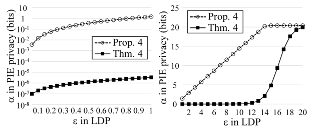
Figure 4: Relation between $\varepsilon$ in LDP and $\alpha$ in PIE privacy ($n=1370637$, $|\mathcal{X}|=10500393$).

Figure 4 shows the relation between $\varepsilon$ in LDP and $\alpha$ in PIE privacy. Here we set $n=1370637$ and $|\mathcal{X}|=10500393$ because these values were used in our experiments using the location data. Figure 4 shows that $\alpha$ in Theorem 4.2 is much smaller than $\alpha$ in Proposition 4.1 for both small $\varepsilon$ ($0.05$ to $1$) and large $\varepsilon$ ($1$ to $20$). For example, when $\varepsilon=0.1$, $1$, and $10$, $\alpha$ in Proposition 4.1 is $\alpha=0.014$, $1.4$, and $14$, respectively, whereas $\alpha$ in Theorem 4.2 is $\alpha=2.0\times 10^{-7}$, $3.3\times 10^{-6}$, and $0.043$, respectively. As the input alphabet size $|\mathcal{X}|$ increases, the difference between two $\alpha$ values becomes larger because the MI loss parameter $\theta_{RR}$ decreases with increase in $|\mathcal{X}|$. In other words, $\alpha$ in Theorem 4.2 is much tighter, especially when $|\mathcal{X}|$ is large. In our experiments, we also show that $\alpha$ in Theorem 4.2 is close to the PSE for a specific identification algorithm.

We also show that the $\varepsilon$-RR has compositionality [28] in that $\alpha$ in (16) increases linearly for multiple personal data:

Theorem 4.3 (Composition of the RR).

Let $\theta_{RR}=\frac{e^{\varepsilon}-1}{|\mathcal{X}|+e^{\varepsilon}-1}$. Assume that a user $U$ has $t\in\mathbb{N}$ personal data and obfuscates each of the data by using the $\varepsilon$-RR. For $i\in[t]$, let $X^{(i)}$ and $Y^{(i)}$ be random variables representing the $i$-th personal data and obfuscated data, respectively. Then the combined release $Y=(Y^{(1)},\cdots,Y^{(t)})$ provides $(\mathcal{U},t\alpha)$-PIE privacy, where $\alpha=\theta_{RR}\min\{\log n,\allowbreak\log|\mathcal{X}|\}$.

Theorem 4.3 upper-bounds the PIE when a user has multiple personal data and obfuscates each of them using the $\varepsilon$-RR. Note that Theorem 4.3 holds irrespective of whether there are correlations between $X^{(1)},\cdots,X^{(t)}$ (see Appendix B for details).

4.3 PIE of the GLH

Next we show a tighter bound on the PIE for the $(g,\varepsilon)$-GLH in Section 2.2:

Theorem 4.4 (PIE of the GLH).

Let $\theta_{GLH}=\frac{e^{\varepsilon}-1}{g+e^{\varepsilon}-1}$. For any distribution $p_{U,X}$, the $(g,\varepsilon)$-GLH satisfies

$$I(U;Y)\leq\theta_{GLH}I(U;X).$$ (17)

Therefore, the $(g,\varepsilon)$-GLH provides $(\mathcal{U},\alpha)$-PIE privacy for any $\mathcal{U}\subseteq\Omega$ such that $|\mathcal{U}|=n$, where

$$\alpha=\theta_{GLH}\min\{\log n,\log|\mathcal{X}|\}.$$ (18)

Theorem 4.4 can be proved in an analogous way to Theorem 4.2 because the $(g,\varepsilon)$-GLH uses the RR after applying random projection to $x\in\mathcal{X}$, as shown in (3).

By (17), the $(g,\varepsilon)$-GLH can decrease the mutual information between a user and personal data by $\theta_{GLH}$. As with $\theta_{RR}$, we call $\theta_{GLH}$ the MI loss parameter. $\alpha$ in Theorem 4.4 is much tighter than $\alpha$ in Proposition 4.1, especially when $g$ is large.

As with the $\varepsilon$-RR, the $(g,\varepsilon)$-GLH also composes (irrespective of whether there are correlations between $X^{(1)},\cdots,X^{(t)}$):

Theorem 4.5 (Composition of the GLH).

Let $\theta_{GLH}=\frac{e^{\varepsilon}-1}{g+e^{\varepsilon}-1}$. Assume that a user $U$ has $t\in\mathbb{N}$ personal data and obfuscates each of the data by using the $(g,\varepsilon)$-GLH. For $i\in[t]$, let $X^{(i)}$ and $Y^{(i)}$ be random variables representing the $i$-th personal data and obfuscated data, respectively. Then the combined release $Y=(Y^{(1)},\cdots,Y^{(t)})$ provides $(\mathcal{U},t\alpha)$-PIE privacy, where $\alpha=\theta_{GLH}\min\{\log n,\allowbreak\log|\mathcal{X}|\}$.

Relation between the MI Loss Parameter and the Bayes Error Probability.  In both the RR and GLH, we can set the MI loss parameter to achieve a required identification error probability.

For example, assume that each user sends a single personal datum (i.e., $U$ is uniform) and that we require the Bayes error probability to be $\beta_{U|\mathbf{S}}>0.5$. By Proposition 3.7 and Theorem 4.2 (resp. Theorem 4.4), this requirement is satisfied by setting the MI parameter to $\theta_{RR}=0.5$ (resp. $\theta_{GLH}=0.5$) when $n$ is large.

4.4 Utility Analysis

Finally, we analyze the utility of the $\varepsilon$-RR and the $(g,\varepsilon)$-GLH. Here as with [45, 86, 58], we assume that each user sends a single datum and consider distribution estimation as a task for a data collector.

Preliminaries.  For $i\in[n]$, let $X_{i}$ and $Y_{i}$ be random variables representing user $u_{i}$’s personal data and obfuscated data, respectively. Let $\mathbf{X}_{1:n}=(X_{1},\cdots,X_{n})$ and $\mathbf{Y}_{1:n}=(Y_{1},\cdots,Y_{n})$. Let $\mathcal{C}$ be the probability simplex, and $\mathbf{p}\in\mathcal{C}$ be an empirical distribution of $\mathbf{X}_{1:n}$, whose probability of $x\in\mathcal{X}$ is given by $\mathbf{p}(x)$. In distribution estimation, the data collector estimates $\mathbf{p}$ from $\mathbf{Y}_{1:n}$.

For estimating $\mathbf{p}$ from $\mathbf{Y}_{1:n}$, we use an empirical estimator in the same way as [3, 42, 45, 86, 58] because it is easy to analyze. Let $\hat{\mathbf{p}}_{RR}$ be an empirical estimate of $\mathbf{p}$ when the $\varepsilon$-RR is used. Simple calculations from (2) show that:

$$\hat{\mathbf{p}}_{RR}(x)=\frac{1}{\mu_{RR}-\nu_{RR}}\left(\frac{\mathbf{c}_{RR}(x)}{n}-\nu_{RR}\right),$$ (19)

where $\mu_{RR}=\frac{e^{\varepsilon}}{|\mathcal{X}|+e^{\varepsilon}-1}$, $\nu_{RR}=\frac{1}{|\mathcal{X}|+e^{\varepsilon}-1}$, and $\mathbf{c}_{RR}(x)$ is the number of $x\in\mathcal{X}$ in $\mathbf{Y}_{1:n}$ (note that $\mathcal{X}=\mathcal{Y}$ in the RR).

Similarly, let $\hat{\mathbf{p}}_{GLH}$ be an empirical estimate of $\mathbf{p}$ when the $(g,\varepsilon)$-GLH is used. Let $\mathcal{Y}_{x}=\{(h,y)\in\mathcal{Y}|y=h(x)\}\subseteq\mathcal{Y}$. Then the empirical estimate $\hat{\mathbf{p}}_{GLH}$ can be written as follows [86]:

$$\hat{\mathbf{p}}_{GLH}(x)=\frac{1}{\mu_{GLH}-\nu_{GLH}}\left(\frac{\mathbf{c}_{GLH}(x)}{n}-\nu_{GLH}\right),$$ (20)

where $\mu_{GLH}=\frac{e^{\varepsilon}}{g+e^{\varepsilon}-1}$, $\nu_{GLH}=\frac{1}{g}$, and $\mathbf{c}_{GLH}(x)$ is the number of $(h,y)\in\mathcal{Y}_{x}$ in $\mathbf{Y}_{1:n}$.

As with [45, 86, 58], we use the expected $l_{2}$ loss between the true probability and the estimate as a utility measure. Specifically, we fix $\mathbf{X}_{1:n}$ (and hence $\mathbf{p}$). Given the estimate $\hat{\mathbf{p}}$ of $\mathbf{p}$, we evaluate:

$$\mathbb{E}[(\mathbf{p}(x)-\hat{\mathbf{p}}(x))^{2}]$$ (21)

for each input symbol $x\in\mathcal{X}$, where the expectation is taken over all possible realizations of $\mathbf{Y}_{1:n}$ (hereinafter we omit the subscript $\mathbf{Y}_{1:n}$ in $\mathbb{E}$). Note that when the empirical estimator is used, the expected $l_{2}$ loss is equal to the variance of $\hat{\mathbf{p}}(x)$ because the empirical estimate is unbiased [45, 86].

Expected $l_{2}$ Loss.  We first show the expected $l_{2}$ loss for the $\varepsilon$-RR and the $(g,\varepsilon)$-GLH:

Proposition 4.6 ($l_{2}$ loss of the RR).

For any $x\in\mathcal{X}$,

$$\mathbb{E}[(\mathbf{p}(x)-\hat{\mathbf{p}}_{RR}(x))^{2}]=\frac{|\mathcal{X}|+e^{\varepsilon}-2}{n(e^{\varepsilon}-1)^{2}}+\frac{\mathbf{p}(x)(|\mathcal{X}|-2)}{n(e^{\varepsilon}-1)}.$$ (22)

Proposition 4.7 ($l_{2}$ loss of the GLH).

For any $x\in\mathcal{X}$,

$$\mathbb{E}[(\mathbf{p}(x)-\hat{\mathbf{p}}_{GLH}(x))^{2}]$$

$$=\frac{(g+e^{\varepsilon}-1)^{2}}{n(e^{\varepsilon}-1)^{2}(g-1)}+\frac{\mathbf{p}(x)(g^{2}-2g-e^{\varepsilon}+1)}{n(e^{\varepsilon}-1)(g-1)}.$$ (23)

The first terms in (22) and (23) are shown in [86] for the task of estimating counts of $x\in\mathcal{X}$ in $\mathcal{X}_{1:n}$ (we need to multiply the values in [86] by $1/n^{2}$ to normalize counts to probabilities). The second terms in (22) and (23) are obtained by simple calculations.

Next we show an optimal parameter $g$ in the $(g,\varepsilon)$-GLH while fixing the bound on $\alpha$. Specifically, by Theorem 4.4, the MI loss parameter $\theta_{GLH}$ ($=\frac{e^{\varepsilon}-1}{g+e^{\varepsilon}-1}$) determines the bound on $\alpha$ for fixed $n$ and $|\mathcal{X}|$. Therefore, we fix $\theta_{GLH}$ and find the optimal $g$ that minimizes the expected $l_{2}$ loss. Note that for a fixed $\theta_{GLH}$ ($=\frac{e^{\varepsilon}-1}{g+e^{\varepsilon}-1}$), $\varepsilon$ increases with increase in $g$.

For a fixed privacy budget $\varepsilon$ in LDP, the optimal $g$ that minimizes the expected $l_{2}$ loss is given by: $g=e^{\varepsilon}+1$ [86]. In contrast, we show that for a fixed $\theta_{GLH}$, a larger $g$ provides better utility:

Theorem 4.8 (Optimal $g$ in the GLH).

For a fixed $\theta_{GLH}$ ($=\frac{e^{\varepsilon}-1}{g+e^{\varepsilon}-1}$), the expected $l_{2}$ loss of the $(g,\varepsilon)$-GLH in (23) is monotonically decreasing in $g$ and

$$\mathbb{E}[(\mathbf{p}(x)-\hat{\mathbf{p}}_{GLH}(x))^{2}]\rightarrow\frac{\mathbf{p}(x)(1-\theta_{GLH})}{n\theta_{GLH}}\hskip 8.53581pt(g\rightarrow\infty).$$ (24)

Recall that $g$ in the $(g,\varepsilon)$-GLH is the output size of the hash function $h:\mathcal{X}\rightarrow[g]$. A larger $g$ preserves more information about the personal data $x\in\mathcal{X}$. Therefore, Theorem 4.8 is intuitive in that compressing the personal data $x$ with a smaller $g$ results in the loss of information about $x$, and hence causes the loss of utility.

RR vs. GLH.  We compare the expected $l_{2}$ loss of the RR with that of the GLH. Here we set the MI loss parameters $\theta_{RR}$ and $\theta_{GLH}$ to the same value ($\theta_{RR}=\theta_{GLH}$) so that the bounds on $\alpha$ in (16) and (18) are the same. We assume that $g$ in the GLH is very large and compare the right side of (22) with the right side of (24).

When $\theta_{RR}=\theta_{GLH}$, the right side of (24) can be written as: $\frac{\mathbf{p}(x)(1-\theta_{GLH})}{n\theta_{GLH}}=\frac{\mathbf{p}(x)(1-\theta_{RR})}{n\theta_{RR}}=\frac{\mathbf{p}(x)|\mathcal{X}|}{n(e^{\varepsilon}-1)}$, where $\varepsilon$ satisfies $\theta_{RR}=\frac{e^{\varepsilon}-1}{|\mathcal{X}|+e^{\varepsilon}-1}$. Then for a large $|\mathcal{X}|$, we obtain:

$$\text{the right side of (\ref{eq:optimal_g})}\approx\text{the second term in (\ref{eq:l2_RR})}.$$

Therefore, the remaining question is how large the first term in (22) is compared to the second term in (22).

As an example, we consider the case where $\theta_{RR}=\theta_{GLH}=0.5$ (which guarantees the Bayes error probability $\beta_{U|\mathbf{S}}$ to be larger than $0.5$). In this case, simple calculations show that the first and second terms in (22) are almost equal to $\frac{2}{n|\mathcal{X}|}$ and $\frac{\mathbf{p}(x)}{n}$, respectively. For a popular symbol $x\in\mathcal{X}$ with a large probability $\mathbf{p}(x)\gg\frac{1}{|\mathcal{X}|}$, we obtain $\frac{2}{n|\mathcal{X}|}\ll\frac{\mathbf{p}(x)}{n}$. Therefore, the RR and GLH have almost the same utility for estimating the probabilities for popular symbols $x\in\mathcal{X}$; i.e., heavy hitters [7, 15, 31, 41, 63].

For an unpopular symbol $x\in\mathcal{X}$ with a small probability $\mathbf{p}(x)\ll\frac{1}{|\mathcal{X}|}$, we obtain $\frac{2}{n|\mathcal{X}|}\gg\frac{\mathbf{p}(x)}{n}$. This means that the RR has much larger $l_{2}$ loss for the unpopular symbol. This is caused by the fact negative values are assigned to many unpopular symbols in the RR [3]. However, zero (or very small positive) values can be assigned to the estimates $\hat{\mathbf{p}}(x)$ below a significance threshold (determined via Bon-ferroni correction) [31]. Then both the RR and GLH would have small $l_{2}$ losses for unpopular symbols.

In our experiments, we show that the RR and GLH have almost the same utility for both popular and unpopular symbols when we use the significant threshold. We also note that the communication cost of the RR and GLH can be expressed as $O(\log|\mathcal{X}|)$ and $O(\log g)$, respectively. When $|\mathcal{X}|<g$, the RR is better than the GLH in terms of the communication cost.

4.5 Implications for Privacy and Utility

Theorem 4.8 indicates that a larger $g$ results in a smaller $l_{2}$ loss when $(\mathcal{U},\alpha)$-PIE privacy is used as a privacy metric. On the other hand, the optimal value of $g$ that minimizes the $l_{2}$ loss is $g=e^{\varepsilon}+1$ [86] when $\varepsilon$-LDP is used as a privacy metric. This is counter-intuitive because reducing $g$ from a larger value to $e^{\varepsilon}+1$ decreases the $l_{2}$ loss. In other words, compressing the personal data $x$ with a smaller $g$ results in higher utility until $g=e^{\varepsilon}+1$.

One explanation for this counter-intuitive result is as follows. LDP is data privacy that makes the original data $X$ indistinguishable from any other possible data in $\mathcal{X}$. Here it becomes more difficult to guarantee the indistinguishability as the size $|\mathcal{X}|$ of the data domain increases. Thus, for a fixed $\varepsilon$, a larger $|\mathcal{X}|$ results in lower utility. In fact, by (2), the RR with the same $\varepsilon$ requires more noise for a larger $|\mathcal{X}|$. A similar phenomenon occurs in matrix factorization under LDP [68] – a large amount of noise is added in [68] due to high dimensionality of data. This is caused by the fact that LDP guarantees the indistinguishability of data. One way to increase the utility while fixing $\varepsilon$ is dimension reduction; i.e., reducing the value of $g$ (dimension reduction is also adopted in [68]). It should be noted, however, that too small $g$ results in a significant loss of information about the personal data $x$. The optimal $g$, which balances these two effects, is $g=e^{\varepsilon}+1$.

Our PIE privacy has a different implication for privacy and utility. PIE privacy is user privacy that aims to prevent the identification of $U$ (rather than the inference of $X$) by bounding $I(U;Y)$. Consequently, the MI loss parameter $\theta_{GLH}$ $(=\frac{e^{\varepsilon}-1}{g+e^{\varepsilon}-1})$ in the GLH does not depend on $|\mathcal{X}|$. Therefore, for a fixed $\theta_{GLH}$, dimension reduction only results in the loss of information about $x$. This explains the reason for an intuitive result that a larger $g$ provides better utility in our notion.

5 Experimental Evaluation

We proposed the PIE as a measure of re-identification risks in the local model, and analyzed the PIE and utility for the RR and GLH. Based on this, we would like to pose the following two basic questions: 1) How identifiable are personal data such as location traces and rating history? 2) Is the PIE able to guarantee low re-identification risks for local obfuscation mechanisms such as the RR and GLH while keeping high utility? We conducted experiments to answer to these questions.

5.1 Experimental Set-up

In our experiments, we used five large-scale datasets:

Location Trace.  As a location trace dataset (denoted by LT), we used the Foursquare dataset (Global-scale Check-in Dataset with User Social Networks) [89]. This dataset includes $90048627$ check-ins by $2733324$ users on POIs all over the world. Each check-in is associated with its timestamp. We extracted $1370637$ users who had at least $10$ check-ins. The total number of POIs checked in by these users was $10500393$; i.e., $|\mathcal{U}|=1370637$, $|\mathcal{X}|=10500393$.

For each user $u_{i}\in\mathcal{U}$, we divided the location trace (time-series check-in data) into two disjoint traces of the same size. We used the former trace as training data in the partial-knowledge model, and the latter trace as personal data $X$. We used the training data of user $u_{i}$ as auxiliary information $r_{i}$ available to the adversary.

Rating History.  As a rating history dataset (denoted by RH), we used the MovieLens Latest dataset [55], which includes $27753444$ ratings by $283228$ users. Ratings are made on a 5-star scale with half-star increments ($0.5$ to $5$). Each rating is associated with its timestamp. We used $4$ to $5$ star ratings that represent “likes” and extracted $185107$ users who provided at least $10$ such ratings. The total number of movies rated by these users was $58098$; i.e., $|\mathcal{U}|=185107$, $|\mathcal{X}|=58098$.

Since each user rates each movie at most once, it is difficult for the adversary to identify a user based on training data completely separated from personal data $X$. Therefore, for each user $u_{i}\in\mathcal{U}$, we used the whole rating history (time-series rating data) as personal data $X$, and used the first $1$ to $5$ events (ratings) in $X$ as training data in the partial-knowledge model.

Face.  The NIST BSSR1 Set3 dataset [61] includes face scores (similarities) from $3000$ users; i.e., $|\mathcal{U}|=3000$. Face scores were calculated by two matchers (“C” and “G”). We used scores from the matcher G because some users had inappropriate scores ($=-1$) in the matcher C. We used $3000\times 3000$ scores in total. The face matcher G has lower errors than the best matcher in the FRPC 2017 [39], as described in Section 5.2 in detail.

Fingerprint.  The CASIA-FingerprintV5 dataset [14] (denoted by FP) includes $20000$ fingerprint images of $4000$ fingers ($5$ images per finger). We assumed that each finger was presented by a different user; i.e., $|\mathcal{U}|=4000$. For each finger, we used the first and second images as a template and biometric data presented at authentication, respectively. To calculate a score between two fingerprint images, we used the VeriFinger SDK 7.0 [84], a state-of-the-art commercial fingerprint matcher. We extracted $4000\times 4000$ scores in total.

Finger-Vein.  The finger-vein dataset in [88] (denoted by FV) includes $33330$ finger-vein images of $3030$ fingers ($11$ images per finger); i.e., $|\mathcal{U}|=3030$. For each finger, we used two images as a template and biometric data at authentication, respectively. To calculate a score, we used the CIRF (Correlation Invariant Random Filtering) [73, 75]. We used $3030\times 3030$ scores between the transformed finger-vein features.

To calculate scores in LT and RH, we used the matching algorithm based on the Markov chain model, because this model is effective for location privacy attacks [37, 56, 57, 70] and personalized item recommendation [64, 12]. Specifically, we trained a transition matrix $\Lambda_{i}\in[0,1]^{|\mathcal{X}|\times|\mathcal{X}|}$ for each user $u_{i}$ from training data via the MLE (Maximum Likelihood Estimation). We also trained a visit probability vector $\mathbf{\pi}_{i}\in\mathcal{C}$, which represents a probability distribution of personal data in $\mathcal{X}$, for each user $u_{i}$ via the MLE; i.e., $\mathbf{\pi}_{i}$ is an empirical distribution of the training data. The auxiliary information $r_{i}$ of the user $u_{i}$ can be expressed as: $r_{i}=(\Lambda_{i},\mathbf{\pi}_{i})$. Given obfuscated data $Y$ and $r_{i}$, we calculated a likelihood that $Y$ belongs to $u_{i}$ as follows. We calculated the likelihood for the first event in $Y$ via $\mathbf{\pi}_{i}$ and for the subsequent events in $Y$ via $\Lambda_{i}$. Then we multiplied them to obtain the likelihood for $Y$. Here we assigned a small positive value ($=10^{-8}$) to zero elements in $\Lambda_{i}$ and $\mathbf{\pi}_{i}$ so that the likelihood never becomes $0$ [56, 57]. We used the likelihood for $Y$ as a score $s_{i}$.

Based on genuine scores (scores for the same user) and impostor scores (scores for different users) for $|\mathcal{U}|$ users, we evaluated the PSE by estimating $D(f_{G}||f_{I})$. Note that $D(f_{G}||f_{I})$ measures the PSE for a very large value of $n$ (when $n$ goes to infinity), as in Theorem 3.2. To estimate $D(f_{G}||f_{I})$, we used the generalized $k$-NN estimator [85] because it is asymptotically unbiased; i.e., it converges to the true value as the sample size increases. We also confirmed that for each dataset, $D(f_{G}||f_{I})$ converges as the number of users increases.

5.2 Results for No Obfuscation Cases

We first evaluated the identifiability of personal data when no obfuscation mechanisms were used. Figure 5 shows the PSE in the maximum-knowledge model [25, 67] where the adversary uses personal data $X$ (the latter half of the trace in LT and the whole rating history in RH) as training data. In the left figure, each user sends $X$ without obfuscation; i.e., $Y=X$. In the right figure, each user sends the first $1$ to $5$ events in $X$ as $Y$. We note again that we measure the PSE for a very large value of $n$ (when $n$ goes to infinity); e.g., in Figure 5, the PSE of FV is larger than $\log 3030=11.6$.

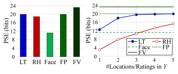
Figure 5: PSE in the maximum-knowledge attacker model. In LT and RH, the adversary uses $X$ as training data. Then in the left figure, each user sends $X$ without obfuscation ($Y=X$). In the right figure, each user sends the first $1$ to $5$ events in $X$ as $Y$.

The left figure shows that LT and RH have almost the same identifiability as the commercial fingerprint matcher (FP) in the maximum-knowledge model. Moreover, the right figure shows that only three locations are enough to have almost the same identifiability as a fingerprint. This is consistent with the fact that only three locations are enough to uniquely characterize about $80\%$ of individuals among one and a half million people [22].

Although the maximum-knowledge model reflects the worst-case scenario where the maximum auxiliary information is available to the adversary, it may not be realistic. For example, it is natural to consider that the whole location trace $X$ is not available as auxiliary information in practice (unless the adversary tracks the user all the time). In this case, even if $X$ is highly unique (as shown in [22] for location data), it might be difficult for the adversary to identify a user.

Therefore, we evaluated the identifiability of LT and RH in the partial-knowledge model. In LT, we extracted $1896$ users who had at least $1000$ check-ins. Then for each user, we used the former half of the trace as training data, and the latter half of the trace as personal data $X$. We changed the number of training events (locations) from $100$ to $500$. In RH, we extracted $1888$ users who had at least $500$ ratings with $4$ to $5$ stars. Then we used the first $1$ to $5$ events (ratings) in $X$ as training data. In both LT and RH, we used no obfuscation mechanisms ($Y=X$).

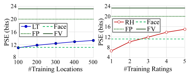
Figure 6: PSE in the partial-knowledge attacker model. In LT, the adversary uses training data separated from $X$. In RH, the adversary uses the first $1$ to $5$ ratings in $X$ as training data. Then each user sends $X$ without no obfuscation; i.e., $Y=X$.

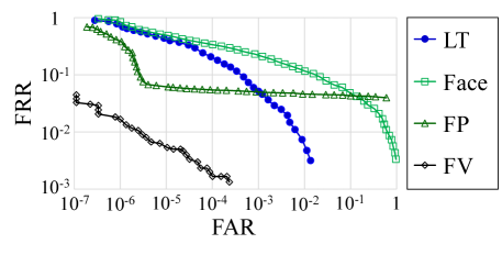
Figure 7: DET curve in the partial-knowledge attacker model. In LT, the number of training locations is $500$.

Figure 6 shows the results. In both LT and RH, the PSE increases with increase in the number of training events. The PSE of LT (resp. RH) is larger than that of the face matcher in [61] when the number of training events is larger than or equal to $200$ (resp. $3$). We emphasize that although a part of $X$ was used as training data in RH, the training data in LT was completely separated from $X$.

We also evaluated FAR (False Acceptance Rate) and FRR (False Rejection Rate), commonly used accuracy measures in biometrics [9, 43]. FAR (resp. FRR) is the proportion of verification attempts in which the system incorrectly accepts an impostor (resp. rejects a genuine user). In the local privacy model, FAR (resp. FRR) corresponds to the error rates in which, given auxiliary information $r_{i}$ of some user, the adversary incorrectly decides that obfuscated data $Y$ and $r_{i}$ belong to the same user (resp. different users). We evaluated the DET (Detection Error Tradeoff) curve [52], which is obtained by plotting FAR against FRR at various thresholds, using genuine and impostor scores for $|\mathcal{U}|$ users.

Figure 7 shows the DET curve of LT in the partial-knowledge model ($500$ training locations) and biometric data. This figure shows that LT provides smaller FAR and FRR than the face, which is consistent with the PSE in Figure 6.

We also note that the best matcher in the FRPC (Face Recognition Prize Challenge) 2017 [39] had FRR of about $0.15$ (resp. $0.1$) at FAR of $0.01$ (resp. $0.1$), which is worse than that of the face matcher in Figure 7. The high FAR and FRR in the FRPC 2017 were caused by the fact that face images were collected without tight quality constraints. In particular, unconstrained yaw and pitch pose variation caused errors [39]. Similarly, Figure 7 shows that FRR of FP is high (even using the commercial fingerprint matcher). This is because users were asked to rotate their fingers with various levels of pressure in the CASIA-FingerprintV5 dataset [14].

In summary, our answers to the first question at the beginning of Section 5 are as follows:

• Three locations are enough to have almost the same identifiability as the commercial fingerprint matcher in the maximum-knowledge model (ratings need more events).

• A long location trace ($\geq 500$ locations) has higher identifiability than the face matcher in [11] and the best face matcher in the FRPC 2017 [39] in the partial-knowledge model where training data is separated from $X$.

We emphasize that the second answer illustrates an interesting feature of our PSE that provides a new intuitive understanding of re-identification risks; i.e., a long location trace is more identifiable than the best face matcher in the prize challenge. For example, the EU’s AI Act [32] states that (both ‘real-time’ and ‘post’) remote biometric identification systems should be classified as high-risk. Based on the second answer, we argue that systems collecting location traces should also be considered as high-risk in terms of the re-identification risk.

5.3 Results for the RR and GLH

Next we evaluated the privacy and utility of the RR and GLH. Here we focused on LT because it has higher identifiability than RH as shown in Figure 5.

We used location traces of all users ($|\mathcal{U}|=1370637$). We assumed that each user obfuscates the first location $X$ in the latter half of the trace using the RR or GLH, and sends the obfuscated location $Y$ to a data collector. In other words, we assumed that each user sends a single datum as in Section 4.4. Note that a single location may be enough to identify a user, as shown in Figure 5. For example, a user’s home or work location is highly identifiable information [38]. We also note that the privacy of the RR and GLH in the case of multiple obfuscated data can be discussed based on the composition theorems (Theorems 4.3 and 4.5).

We first examined how tight our upper-bounds on the PIE for the RR and GLH (Theorems 4.2 and 4.4) are. To this end, we evaluated the PSE, which lower-bounds the PIE (Proposition 3.3). As training data of the adversary, we used the former half of the trace; i.e., partial-knowledge model.

Figure 9 shows the upper-bounds ($\alpha$ in Proposition 4.1, Theorem 4.2, and Theorem 4.4) and lower-bounds (PSE) on the PIE. Here we set $g$ in the GLH to $g=10^{8}$. Figure 9 shows that the values of $\alpha$ in Theorems 4.2 and 4.4 are much smaller than $\alpha$ in Proposition 4.1, and are close to the PSE. This indicates that our upper-bounds for the RR and GLH in Theorems 4.2 and 4.4 are fairly tight and cannot be improved much.

We also examined how tight the lower-bounds on the identification error probability $\beta_{U|\mathbf{S}}$ in Proposition 3.7 are. To this end, we performed the re-identification attack for each obfuscated location $Y$ using the matching algorithm based on the Markov chain model and the best score rule (described in Section 3.1). Then we evaluated the identification error rate, which is the proportion of correct identification results.

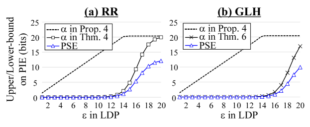
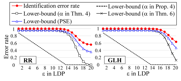
Figure 8: Upper-bounds ($\alpha$ in Proposition 4.1 and Theorems 4.2 and 4.4) and lower-bounds (PSE) on the PIE in the $\varepsilon$-RR and $(g,\varepsilon)$-GLH ($g=10^{8}$).

Figure 9: Identification error rate in the $\varepsilon$-RR and $(g,\varepsilon)$-GLH ($g=10^{8}$). The lower-bounds (blue and black lines) are obtained by assigning $\alpha$ (resp. PSE) in Figure 9 to (12) (resp. (10)).

Figure 9 shows the results. Here the lower-bounds on $\beta_{U|\mathbf{S}}$ are obtained by assigning $\alpha$ (resp. PSE) in Figure 9 to (12) (resp. (10)). Figure 9 shows that the gap between the identification error rate and the lower-bound is caused by two factors. Specifically, the gap between “Identification error rate” (red line) and “Lower-bound (PSE)” (blue line) is caused by the generalized Fano’s inequality [40]; i.e., the first inequality in (10). The gaps between “Lower-bound (PSE)” (blue line) and the other lower-bounds (black lines) are caused by the gap between the PSE and $\alpha$ in PIE privacy ($\alpha$ in Proposition 4.1 and Theorems 4.2 and 4.4). Figure 9 also shows that the lower-bounds by Theorem 4.2 and 4.4 are much tighter than the lower-bound by Proposition 4.1.

Finally, we evaluated the utility. As a task for a data collector, we considered distribution estimation. For a distribution estimation method, we used the empirical estimator without a significant threshold (denoted by emp) and the empirical estimator with a significant threshold [31] (denoted by emp+thr). In emp+thr, we set the significance level to $0.05$ in the same way as [31, 58, 86], and assigned zero to probabilities below a significance threshold. Then we evaluated the sum of $l_{2}$ losses $(\mathbf{p}(x)-\hat{\mathbf{p}}(x))^{2}$ over the top $\phi\in\{100,|\mathcal{X}|\}$ POIs whose probabilities $\mathbf{p}(x)$ are the largest. The top $\phi=100$ POIs correspond to heavy hitters.

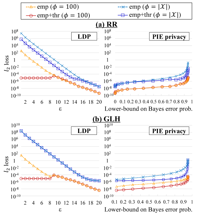
Figure 10: Sum of the $l_{2}$ losses over the top $\phi\in\{100,|\mathcal{X}|\}$ POIs with various values of $\varepsilon$ ($g=10^{8}$).

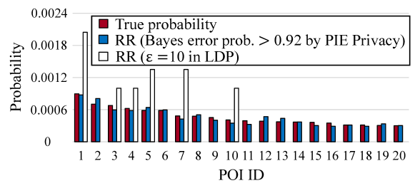
Figure 11: Probabilities of the top-$20$ POIs and estimates by emp+thr. The relative error of the RR with $\beta_{U|\mathbf{S}}>0.92$ guaranteed by PIE privacy (resp. $\varepsilon=10$ in LDP) was $0.10$ (resp. $1.05$)

.

Figure 10 shows the results ($g=10^{8}$). Here the left figures show $\varepsilon$ in LDP, whereas the right figures show the lower-bounds on the Bayes error probability $\beta_{U|\mathbf{S}}$ obtained by PIE privacy (Corollary 3.9 and Theorems 4.2 and 4.4). Figure 10 shows that the utility is improved by using the significant threshold. This is because emp assigns negative values to many input symbols [3]. However, emp+thr still provides poor utility when $\varepsilon\leq 10$. We also show in Figure 11 the probabilities $\mathbf{p}(x)$ of the top-$20$ POIs (red bars) and the estimates $\hat{\mathbf{p}}(x)$ by emp+thr when we use the RR with $\varepsilon=10$ (white bars). The RR with $\varepsilon=10$ performs poorly. The relative error $\frac{|\mathbf{p}(x)-\hat{\mathbf{p}}(x)|}{\mathbf{p}(x)}$ of the RR with $\varepsilon=10$ for each of the top $20$ POIs was on average $1.05$ ($>1$). Note that $\varepsilon=10$ is considered to provide almost no privacy guarantees for personal data [51], because $e^{\varepsilon}$ in (1) is $e^{10}=22026$. This means that LDP fails to guarantee meaningful privacy and utility for this task.

On the other hand, our PIE privacy can be used to prevent re-identification attacks while keeping high utility. For example, Figure 10(a) shows that LDP requires $\varepsilon>12$ (no meaningful privacy guarantees) to achieve the $l_{2}$ loss of $10^{-6}$ using emp+thr ($\phi=100$). In contrast, PIE privacy guarantees the Bayes error probability to be $\beta_{U|\mathbf{S}}>0.92$ with the same $l_{2}$ loss. Figure 11 shows the estimates $\hat{\mathbf{p}}(x)$ by the RR and emp+thr in this case (blue bars). The RR accurately estimates the distribution for the $20$-POIs while satisfying $\beta_{U|\mathbf{S}}>0.92$. The relative error of the RR in this case was $0.10$, which was much smaller than $1$. Therefore, PIE privacy can be used to guarantee the identification error probability larger than $0.92$ while keeping high utility in this task.

We finally set the MI loss parameters in the RR and GLH to $\theta_{RR}=\theta_{GLH}=0.5$ (which guarantees the Bayes error probability $\beta_{U|\mathbf{S}}$ larger than $0.5$), and changed the parameter $g$ in the GLH from $10^{3}$ to $2\times 10^{9}$ while fixing the MI loss parameter $\theta_{GLH}$. Then we evaluated the sum of the $l_{2}$ losses over the top $\phi\in\{100,|\mathcal{X}|\}$ POIs.

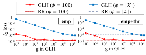
Figure 12: Sum of the $l_{2}$ losses over the top $\phi\in\{100,|\mathcal{X}|\}$ POIs with various values of $g$ when the Bayes error probability $\beta_{U|\mathbf{S}}$ larger than $0.5$ ($\theta_{RR}=\theta_{GLH}=0.5$).

Figure 12 shows the result. In the GLH, the $l_{2}$ loss decreases with increase in $g$, which is consistent with Theorem 4.8. The GLH with a large $g$ has almost the same utility as the RR for $\phi=100$. When we use emp, the GLH with a large $g$ has slightly better utility than the RR for $\phi=|\mathcal{X}|$. However, when we use emp+thr, they have almost the same utility for $\phi=|\mathcal{X}|$ because zero values are assigned to unpopular symbols in both the RR and GLH, as discussed in Section 4.4.

In summary, our answers to the second question at the beginning of Section 5 are as follows:

• Our PIE guarantees the identification error probability larger than $0.92$ while keeping high utility in distribution estimation. On the other hand, LDP destroys the utility even when $\varepsilon=10$.

• Compressing the personal data $X$ with a smaller value of $g$ in the GLH results in the loss of utility for given PIE guarantees, which is consistent with our theoretical results.

6 Conclusion

We proposed the PIE (Personal Information Entropy) as a measure of re-identification risks in the local model. We conducted experiments using five datasets, and showed that a location trace has higher identifiability than the face matcher in [61] and the best matcher in the FRPC 2017 [39] in the partial-knowledge model. We also showed that the PIE can be used to guarantee low re-identification risks for the RR and GLH while keeping high utility in distribution estimation.

As described in Section 1, our PIE privacy is an average notion (though it differs from the re-identification rate in that PIE privacy does not specify an identification algorithm nor the adversary’s background knowledge, as described in Section 3.2). One way to extend our PIE privacy from the average notion to the worse-case notion is to use $\alpha$-mutual information [83], which is an extension of the mutual information using Rényi divergence. Rényi divergence with $\alpha=1$ is equivalent to the KL divergence, whereas Rényi divergence with $\alpha=\infty$ is equivalent to the max divergence, which is a worst-case analog of the KL divergence. Therefore, we can extend our PIE privacy to the the worst-case privacy metric by using $\alpha$-mutual information with a large $\alpha$. Then the following questions remain open: How do the theoretical properties of the PIE (shown in Section 3.3) change? How do the bounds on privacy and utility for obfuscation mechanisms (e.g., RR, GLH) change? As future work, we would like to investigate these open questions.

Appendix A Proofs of Statements in Section 3

Proof A.1 (Proof of Theorem 3.5 (Post-processing invariance)).

Let $\mathcal{Y}^{\prime}$ be the range of the randomized algorithm $\lambda$, and $Y^{\prime}$ be a random variable representing obfuscated data output by $\lambda\circ\mathbf{Q}$.

The obfuscation mechanism $\mathbf{Q}$ takes as input personal data $X$ of a user $U$ and outputs $Y$. Then the randomized algorithm $\lambda$ takes as input $Y$ and outputs $Y^{\prime}$. Thus, $U$, $X$, $Y$ and $Y^{\prime}$ form the Markov chain; i.e., $U\rightarrow X\rightarrow Y\rightarrow Y^{\prime}$. Then by the data processing inequality [20] and (5), we obtain:

$$I(U;Y^{\prime})\leq I(U;Y)\leq\alpha~{}~{}(bits).$$

Therefore, $\lambda\circ\mathbf{Q}$ provides $(n,\alpha)$-PIE privacy.

Proof A.2 (Proof of Theorem 3.6 (Convexity)).

Let $Y_{w}$, $Y_{1}$, and $Y_{2}$ be random variables representing obfuscated data output by $\mathbf{Q}_{w}$, $\mathbf{Q}_{1}$, and $\mathbf{Q}_{2}$, respectively. Given a user $U$, let $p_{X|U}$, $p_{Y_{w}|U}$, $p_{Y_{1}|U}$, $p_{Y_{2}|U}$ be a probability distribution of $X$, $Y_{w}$, $Y_{1}$, and $Y_{2}$, respectively. Then the probability of outputting $y$ from $\mathbf{Q}_{w}$ is written as follows:

$$p_{Y_{w}|U}(y) =\sum_{x\in\mathcal{X}}\mathbf{Q}_{w}(y|x)p_{X|U}(x)$$

$$=\sum_{x\in\mathcal{X}}\left(w\mathbf{Q}_{1}(y|x)+(1-w)\mathbf{Q}_{2}(y|x)\right)p_{X|U}(x)$$

$$=wp_{Y_{1}|U}(y)+(1-w)p_{Y_{2}|U}(y).$$ (25)

The mutual information $I(U;Y_{w})$ is convex in $p_{Y_{w}|U}$ (see Theorem 2.7.4 in [20]). In addition, $I(U;Y_{1})\leq\alpha$ and $I(U;Y_{2})\leq\alpha$ because $\mathbf{Q}_{1}$ and $\mathbf{Q}_{2}$ provide $(n,\alpha)$-PIE privacy. Then by (25), we obtain:

$$I(U;Y_{w}) \leq wI(U;Y_{1})+(1-w)I(U;Y_{2})$$

$$\leq w\alpha+(1-w)\alpha$$

$$=\alpha.$$

Therefore, $\mathbf{Q}_{w}$ provide $(n,\alpha)$-PIE privacy.

Appendix B Proofs of Statements in Section 4

Proof B.1 (Proof of Proposition 4.1 (LDP and PIE)).

We use the following lemma:

Lemma B.2.

If an obfuscation mechanism $\mathbf{Q}$ provides $\varepsilon$-LDP, then

$$I(X;Y)\leq\min\{\varepsilon\log e,\varepsilon^{2}\log e\}~{}~{}(bits).$$ (26)

This is a special case of Lemma 1 in [21] in the local model. By (13) in Proposition 3.10, (26), and $I(U;X)\leq\min\{\log n,\log|\mathcal{X}|\}$, we obtain:

$$I(U;Y)\leq\min\{\varepsilon\log e,\varepsilon^{2}\log e,\log n,\log|\mathcal{X}|\}.$$

Note that this holds for any distribution $p_{U,X}$. Thus Proposition 4.1 holds.

Proof B.3 (Proof of Theorem 4.2 (PIE of the RR)).

Let $p_{U}$ be a probability distribution of $U$. Let $p_{Y}$ be a probability distribution of $Y$, and $p_{Y|U=u_{i}}$ be a conditional probability distribution of $Y$ given $U=u_{i}$. Then $I(U;Y)$ can be written as follows:

$$I(U;Y)=\sum_{i=1}^{n}p_{U}(u_{i})D(p_{Y|U=u_{i}}||p_{Y}).$$ (27)

Let $p_{\text{uni}}$ be a uniform distribution over $\mathcal{X}$; i.e., $p_{\text{uni}}(x)=\frac{1}{|\mathcal{X}|}$ for any $x\in\mathcal{X}$. Let $p_{X}$ be a probability distribution of $X$, and $p_{X|U=u_{i}}$ be a conditional probability distribution of $X$ given $U=u_{i}$. By (2), we can regard the $\varepsilon$-RR as a mechanism that given $x\in\mathcal{X}$, outputs $y=x$ with probability $\theta_{RR}$ ($=\frac{e^{\varepsilon}-1}{|\mathcal{X}|+e^{\varepsilon}-1}$) and outputs a value randomly chosen from $\mathcal{X}$ (including $x$) with probability $1-\theta_{RR}$. Therefore, given $U=u_{i}$, $Y$ is generated from $p_{X|U=u_{i}}$ with probability $\theta_{RR}$, and is generated from $p_{\text{uni}}$ with probability $1-\theta_{RR}$. Then we obtain:

$$D(p_{Y|U=u_{i}}||p_{Y})$$

$$=D(\theta_{RR}p_{X|U=u_{i}}+(1-\theta_{RR})p_{\text{uni}}||\theta_{RR}p_{X}+(1-\theta_{RR})p_{\text{uni}})$$

$$\leq\theta_{RR}D(p_{X|U=u_{i}}||p_{X})+(1-\theta_{RR})D(p_{\text{uni}}||p_{\text{uni}})$$

(by the convexity of the KL divergence [20])

$$=\theta_{RR}D(p_{X|U=u_{i}}||p_{X}).$$ (28)

By (27) and (28), we obtain:

$$I(U;Y) \leq\sum_{i=1}^{n}p_{U}(u_{i})\theta_{RR}D(p_{X|U=u_{i}}||p_{X})$$

$$=\theta_{RR}\sum_{i=1}^{n}p_{U}(u_{i})D(p_{X|U=u_{i}}||p_{X})$$

$$=\theta_{RR}I(U;X).$$ (29)

Therefore, (15) holds. Note that this holds for any distribution $p_{U,X}$. (16) is immediately derived from (15) because $I(U;X)\leq H(U)\leq\log n$ and $I(U;X)\leq H(X)\leq\log|\mathcal{X}|$.

Proof B.4 (Proof of Theorem 4.3 (Composition of the RR)).

For $i\in[t]$, let $\mathbf{Y}^{i}=(Y^{(1)},\cdots,Y^{(i)})$. Then, by the chain rule for the mutual information [20], we obtain:

$$I(U;Y)=I(U;Y^{(1)})+\sum_{i=2}^{t}I(U;Y^{(i)}|\mathbf{Y}^{i-1}).$$ (30)

Let $p_{U}$ and $p_{\mathbf{Y}^{i}}$ be a probability distribution of $U$ and $\mathbf{Y}^{i}$, respectively. Let $p_{Y^{(i)}|U=u_{i},\mathbf{Y}^{i-1}=\mathbf{y}^{i-1}}$ (resp. $p_{Y^{(i)}|\mathbf{Y}^{i-1}=\mathbf{y}^{i-1}}$) be a conditional probability distribution of $Y^{(i)}$ given $U=u_{i}$ and $\mathbf{Y}^{i-1}=\mathbf{y}^{i-1}$ (resp. given $\mathbf{Y}^{i-1}=\mathbf{y}^{i-1}$). Then $I(U;Y^{(i)}|\mathbf{Y}^{i-1})$ in (30) can be written as follows:

$$I(U;Y^{(i)}|\mathbf{Y}^{i-1})$$

$$=\sum_{\mathbf{y}^{i-1}\in\mathcal{Y}^{i-1}}p_{\mathbf{Y}^{i-1}}(\mathbf{y}^{i-1})\sum_{i=1}^{n}p_{U}(u_{i}|\mathbf{y}^{i-1})D(p_{Y^{(i)}|U=u_{i},\mathbf{Y}^{i-1}=\mathbf{y}^{i-1}}||p_{Y^{(i)}|\mathbf{Y}^{i-1}=\mathbf{y}^{i-1}}).$$ (31)

Let $p_{\text{uni}}$ be a uniform distribution over $\mathcal{X}$. Let $p_{X^{(i)}|U=u_{i},\mathbf{Y}^{i-1}=\mathbf{y}^{i-1}}$ (resp. $p_{X^{(i)}|\mathbf{Y}^{i-1}=\mathbf{y}^{i-1}}$) be a conditional probability distribution of $X^{(i)}$ given $U=u_{i}$ and $\mathbf{Y}^{i-1}=\mathbf{y}^{i-1}$ (resp. given $\mathbf{Y}^{i-1}=\mathbf{y}^{i-1}$). By (2), the $\varepsilon$-RR takes as input $x\in\mathcal{X}$, and outputs $y=x$ with probability $\theta_{RR}$ ($=\frac{e^{\varepsilon}-1}{|\mathcal{X}|+e^{\varepsilon}-1}$) and outputs a value randomly chosen from $\mathcal{X}$ (including $x$) with probability $1-\theta_{RR}$. Note that this is independent of the other input and output data. In other words, given $X^{(i)}$, the $\varepsilon$-RR outputs $Y^{(1)}=X^{(i)}$ with probability $\theta_{RR}$ and a random value from $\mathcal{X}$ (including $X^{(i)}$) with probability $1-\theta_{RR}$, irrespective of whether there are correlations between $X^{(1)},\cdots,X^{(t)}$. Thus we obtain:

$$D(p_{Y^{(i)}|U=u_{i},\mathbf{Y}^{i-1}=\mathbf{y}^{i-1}}||p_{Y^{(i)}|\mathbf{Y}^{i-1}=\mathbf{y}^{i-1}})$$

$$=D(\theta_{RR}~{}p_{X^{(i)}|U=u_{i},\mathbf{Y}^{i-1}=\mathbf{y}^{i-1}}+(1-\theta_{RR})p_{\text{uni}}||\theta_{RR}~{}p_{X^{(i)}|\mathbf{Y}^{i-1}=\mathbf{y}^{i-1}}+(1-\theta_{RR})p_{\text{uni}})$$

$$\leq\theta_{RR}D(p_{X^{(i)}|U=u_{i},\mathbf{Y}^{i-1}=\mathbf{y}^{i-1}}||p_{X^{(i)}|\mathbf{Y}^{i-1}=\mathbf{y}^{i-1}})$$

$$\hskip 14.22636pt\text{(by the convexity of the KL divergence \cite[cite]{[\@@bibref{}{elements}{}{}]} and $D(p_{\text{uni}}||p_{\text{uni}})=0$)}.$$ (32)

By (31) and (32), we obtain:

$$I(U;Y^{(i)}|\mathbf{Y}^{i-1})$$

$$\leq\sum_{\mathbf{y}^{i-1}\in\mathcal{Y}^{i-1}}p_{\mathbf{Y}^{i-1}}(\mathbf{y}^{i-1})\sum_{i=1}^{n}p_{U}(u_{i}|\mathbf{y}^{i-1})\theta_{RR}D(p_{X^{(i)}|U=u_{i},\mathbf{Y}^{i-1}=\mathbf{y}^{i-1}}||p_{X^{(i)}|\mathbf{Y}^{i-1}=\mathbf{y}^{i-1}})$$

$$=\theta_{RR}I(U;X^{(i)}|\mathbf{Y}^{i-1})$$ (33)

By (30) and (33), we obtain:

$$I(U;Y)\leq\theta_{RR}I(U;X^{(1)})+\sum_{i=2}^{t}\theta_{RR}I(U;X^{(i)}|\mathbf{Y}^{i-1}).$$ (34)

In (34), $I(U;X^{(i)}|\mathbf{Y}^{i-1})\leq H(U|\mathbf{Y}^{i-1})\leq\log n$ and $I(U;X^{(i)}|\allowbreak\mathbf{Y}^{i-1})\leq H(X^{(i)}|\mathbf{Y}^{i-1})\leq\log|\mathcal{X}|$. Therefore, the combined release $Y$ provides $(n,t\alpha)$-PIE privacy, where $\alpha=\theta_{RR}\allowbreak\min\{\log n,\allowbreak\log|\mathcal{X}|\}$.

Proof B.5 (Proof of Theorem 4.4 (PIE of the GLH)).

Let $p_{U}$ be a probability distribution of $U$. Let $p_{Y}$ be a probability distribution of $Y$, and $p_{Y|U=u_{i}}$ be a conditional probability distribution of $Y$ given $U=u_{i}$. Then $I(U;Y)$ can be written as follows:

$$I(U;Y)=\sum_{i=1}^{n}p_{U}(u_{i})D(p_{Y|U=u_{i}}||p_{Y}).$$ (35)

The $(g,\varepsilon)$-GLH outputs $(h,y)\in\mathcal{Y}$ with probability in (3). We denote the probability that the $(g,\varepsilon)$-GLH outputs $h$, $y$, and $(h,y)$ simply by $\Pr(h)$, $\Pr(y)$, and $\Pr(h,y)$, respectively. Then, $D(p_{Y|U=u_{i}}||p_{Y})$ in (35) can be written as follows:

$$D(p_{Y|U=u_{i}}||p_{Y})$$

$$=\sum_{(h,y)\in\mathcal{Y}}\Pr(h,y|U=u_{i})\log\frac{\Pr(h,y|U=u_{i})}{\Pr(h,y)}$$

$$=\sum_{h\in\mathcal{H}}\Pr(h)\sum_{y\in[g]}\Pr(y|h,U=u_{i})\log\frac{\Pr(h)\Pr(y|h,U=u_{i})}{\Pr(h)\Pr(y|h)}$$

(by $$\Pr(h|U=u_{i})=\Pr(h)$$)

$$=\sum_{h\in\mathcal{H}}\Pr(h)\sum_{y\in[g]}\Pr(y|h,U=u_{i})\log\frac{\Pr(y|h,U=u_{i})}{\Pr(y|h)}.$$ (36)

Let $q_{\text{uni}}$ be a uniform distribution over $[g]$. Given $x\in\mathcal{X}$, let $z$ be a hash value $z=h(x)\in[g]$, and $Z$ be a random variable representing a hash value. Let $H$ be a random variable representing a hash function. Furthermore, let $p_{Z|H=h,U=u_{i}}$ (resp. $p_{Z|H=h}$) be a conditional probability distribution of $Z$ given $H=h$ and $U=u_{i}$ (resp. given $H=h$). By (3), the $(g,\varepsilon)$-GLH outputs $y=z$ with probability $\theta_{GLH}$ ($=\frac{e^{\varepsilon}-1}{g+e^{\varepsilon}-1}$) and outputs a value randomly chosen from $[g]$ (including $z$) with probability $1-\theta_{GLH}$. Therefore, given $H=h$ and $U=u_{i}$, $Y$ is generated from $p_{Z|H=h,U=u_{i}}$ with probability $\theta_{GLH}$, and is generated from $q_{\text{uni}}$ with probability $1-\theta_{GLH}$. Then $D(p_{Y|U=u_{i}}||p_{Y})$ in (36) can be written as follows:

$$D(p_{Y|U=u_{i}}||p_{Y})$$

$$=\sum_{h\in\mathcal{H}}\Pr(h)D(\theta_{GLH}~{}p_{Z|H=h,U=u_{i}}+(1-\theta_{GLH})q_{\text{uni}}||\theta_{GLH}~{}p_{Z|H=h}+(1-\theta_{GLH})q_{\text{uni}})$$

$$\leq\sum_{h\in\mathcal{H}}\Pr(h)\theta_{GLH}D(p_{Z|H=h,U=u_{i}}||p_{Z|H=h})$$

(by the convexity of the KL divergence [20] and $$D(q_{\text{uni}}||q_{\text{uni}})=0$$)

$$=\theta_{GLH}\sum_{h\in\mathcal{H}}\Pr(h)D(p_{Z|H=h,U=u_{i}}||p_{Z|H=h}).$$ (37)

Note that by expanding $I(U;H,Z)$ in the same way as (35) and (36), $I(U;H,Z)$ can be expressed as follows:

$$I(U;H,Z)$$

$$=\sum_{i=1}^{n}p_{U}(u_{i})\sum_{h\in\mathcal{H}}\Pr(h)\sum_{z\in[g]}\Pr(z|h,U=u_{i})\log\frac{\Pr(z|h,U=u_{i})}{\Pr(z|h)}$$

$$=\sum_{i=1}^{n}p_{U}(u_{i})\sum_{h\in\mathcal{H}}\Pr(h)D(p_{Z|H=h,U=u_{i}}||p_{Z|H=h}).$$ (38)

By (35), (37), and (38), $I(U;Y)$ can be written as follows:

$$I(U;Y)$$

$$\leq\theta_{GLH}I(U;H,Z)$$

$$\leq\theta_{GLH}I(U;X)\hskip 5.69054pt\text{(by the data processing inequality \cite[cite]{[\@@bibref{}{elements}{}{}]}).}$$ (39)

Therefore, (17) holds. This holds for any distribution $p_{U,X}$. (18) also holds because $I(U;X)\leq H(U)\leq\log n$ and $I(U;X)\leq H(X)\leq\log|\mathcal{X}|$.

Proof B.6 (Proof of Theorem 4.5 (Composition of the GLH)).

For $i\in[t]$, let $\mathbf{Y}^{i}=(Y^{(1)},\cdots,Y^{(i)})$. Let $H^{(i)}$ and $Z^{(i)}$ be random variables representing the $i$-th hash function and hash value, respectively.

By the chain rule for the mutual information [20], we obtain:

$$I(U;Y)=I(U;Y^{(1)})+\sum_{i=2}^{t}I(U;Y^{(i)}|\mathbf{Y}^{i-1}).$$ (40)

In the proof of Theorem 4.3, we showed (31), (32), and (33). They differ from (27), (28), and (29), respectively, in that they add $\mathbf{Y}^{i-1}$ as a condition. Similarly, by adding $\mathbf{Y}^{i-1}$ as a condition in (35), (36), (37), and (38), we can show the following inequality:

$$I(U;Y^{(i)}|\mathbf{Y}^{i-1})$$

$$\leq\theta_{GLH}I(U;H^{(i)},Z^{(i)}|\mathbf{Y}^{i-1})$$

$$\leq\theta_{GLH}I(U;X^{(i)}|\mathbf{Y}^{i-1})$$

(by the data processing inequality [20]). (41)

By (40) and (41), we obtain:

$$I(U;Y)\leq\theta_{GLH}I(U;X^{(1)})+\sum_{i=2}^{t}\theta_{GLH}I(U;X^{(i)}|\mathbf{Y}^{i-1}).$$ (42)

In (42), $I(U;X^{(i)}|\mathbf{Y}^{i-1})\leq H(U|\mathbf{Y}^{i-1})\leq\log n$ and $I(U;X^{(i)}|\allowbreak\mathbf{Y}^{i-1})\leq H(X^{(i)}|\mathbf{Y}^{i-1})\leq\log|\mathcal{X}|$. Therefore, the combined release $Y$ provides $(n,t\alpha)$-PIE privacy, where $\alpha=\theta_{GLH}\allowbreak\min\{\log n,\allowbreak\log|\mathcal{X}|\}$.

Proof B.7 (Proof of Proposition 4.6 ($l_{2}$ loss of the RR)).

Let $\hat{\mathbf{p}}_{RR}^{*}(x)=\mathbb{E}[\hat{\mathbf{p}}_{RR}(x)]$. Then the expected $l_{2}$ loss can be written as follows:

$$\mathbb{E}[(\mathbf{p}(x)-\hat{\mathbf{p}}_{RR}(x))^{2}]$$

$$=\mathbb{E}\left[((\hat{\mathbf{p}}_{RR}(x)-\hat{\mathbf{p}}_{RR}^{*}(x))+(\hat{\mathbf{p}}_{RR}^{*}(x)-\mathbf{p}(x)))^{2}\right]$$

$$=\mathbb{E}\left[(\hat{\mathbf{p}}_{RR}(x)-\hat{\mathbf{p}}_{RR}^{*}(x))^{2}\right]+(\hat{\mathbf{p}}_{RR}^{*}(x)-\mathbf{p}(x)))^{2}$$

$$\hskip 8.53581pt+2(\hat{\mathbf{p}}_{RR}^{*}(x)-\mathbf{p}(x))\mathbb{E}\left[(\hat{\mathbf{p}}_{RR}(x)-\hat{\mathbf{p}}_{RR}^{*}(x))\right]$$

$$=\mathbb{E}\left[(\hat{\mathbf{p}}_{RR}(x)-\hat{\mathbf{p}}_{RR}^{*}(x))^{2}\right]+(\hat{\mathbf{p}}_{RR}^{*}(x)-\mathbf{p}(x)))^{2}.$$ (43)

The first term in (43) is the variance, whereas the second term in (43) is the bias. In other words, the expected $l_{2}$ loss consists of the bias and variance, which is called the bias-variance trade-off [59]. It is well known that the empirical estimate is unbiased; i.e., $\hat{\mathbf{p}}_{RR}^{*}(x)=\mathbf{p}(x)$ [45, 86]. Therefore, we obtain:

$$\mathbb{E}[(\mathbf{p}(x)-\hat{\mathbf{p}}_{RR}(x))^{2}] =\mathbb{E}\left[(\hat{\mathbf{p}}_{RR}(x)-\hat{\mathbf{p}}_{RR}^{*}(x))^{2}\right]$$

$$=\mathbb{E}\left[(\hat{\mathbf{p}}_{RR}(x)-\mathbf{p}(x))^{2}\right].$$ (44)

By (19), $\mu_{RR}=\frac{e^{\varepsilon}}{|\mathcal{X}|+e^{\varepsilon}-1}$, and $\nu_{RR}=\frac{1}{|\mathcal{X}|+e^{\varepsilon}-1}$, the right side of (44) can be written as follows:

$$\mathbb{E}\left[(\hat{\mathbf{p}}_{RR}(x)-\mathbf{p}(x))^{2}\right] =\left(\frac{1}{\mu_{RR}-\nu_{RR}}\right)^{2}\frac{\text{Var}[\mathbf{c}_{RR}(x)]}{n^{2}}$$

$$=\left(\frac{|\mathcal{X}|+e^{\varepsilon}-1}{e^{\varepsilon}-1}\right)^{2}\frac{\text{Var}[\mathbf{c}_{RR}(x)]}{n^{2}},$$ (45)

where for $a\in\mathbb{R}$, $\text{Var}[a]$ represents the variance of $a$.

Recall that $\mathbf{c}_{RR}(x)$ is the number of $x\in\mathcal{X}$ in $\mathbf{Y}_{1:n}=(Y_{1},\cdots,Y_{n})$. For $i\in[n]$, let $b_{i}(x)\in\{0,1\}$ be a value that takes $1$ if $Y_{i}=x$ and $0$ if $Y_{i}\neq x$. Then $\mathbf{c}_{RR}(x)=\sum_{i=1}^{n}b_{i}(x)$. By (2), $b_{i}(x)$ is randomly generated from the Bernoulli distribution with parameter $\mu_{RR}$ (resp. $\nu_{RR}$) if $X_{i}=x$ (resp. $X_{i}\neq x$). The number of $x$ in $\mathbf{X}_{1:n}$ is $n\mathbf{p}(x)$, whereas the number of the other input symbols in $\mathbf{X}_{1:n}$ is $n(1-\mathbf{p}(x))$. Therefore, $\text{Var}[\mathbf{c}_{RR}(x)]$ in (45) can be written as follows:

$$\text{Var}[\mathbf{c}_{RR}(x)]$$

$$=n\mathbf{p}(x)\mu_{RR}(1-\mu_{RR})+n(1-\mathbf{p}(x))\nu_{RR}(1-\nu_{RR})$$

$$=\frac{n\mathbf{p}(x)e^{\varepsilon}(|\mathcal{X}|-1)}{(|\mathcal{X}|+e^{\varepsilon}-1)^{2}}+\frac{n(1-\mathbf{p}(x))(|\mathcal{X}|+e^{\varepsilon}-2)}{(|\mathcal{X}|+e^{\varepsilon}-1)^{2}}.$$ (46)

By (44), (45), and (46), we obtain:

$$\mathbb{E}[(\mathbf{p}(x)-\hat{\mathbf{p}}_{RR}(x))^{2}]$$

$$=\frac{\mathbf{p}(x)e^{\varepsilon}(|\mathcal{X}|-1)+(1-\mathbf{p}(x))(|\mathcal{X}|+e^{\varepsilon}-2)}{n(e^{\varepsilon}-1)^{2}}$$

$$=\frac{|\mathcal{X}|+e^{\varepsilon}-2}{n(e^{\varepsilon}-1)^{2}}+\frac{\mathbf{p}(x)e^{\varepsilon}(|\mathcal{X}|-2)-\mathbf{p}(x)(|\mathcal{X}|-2)}{n(e^{\varepsilon}-1)^{2}}$$

$$=\frac{|\mathcal{X}|+e^{\varepsilon}-2}{n(e^{\varepsilon}-1)^{2}}+\frac{\mathbf{p}(x)(|\mathcal{X}|-2)}{n(e^{\varepsilon}-1)}.$$

Therefore (22) holds.

Proof B.8 (Proof of Proposition 4.7 ($l_{2}$ loss of the GLH)).

As with (44), the expected $l_{2}$ loss of the GLH is equal to the variance of the GLH:

$$\mathbb{E}[(\mathbf{p}(x)-\hat{\mathbf{p}}_{GLH}(x))^{2}] =\mathbb{E}\left[(\hat{\mathbf{p}}_{GLH}(x)-\mathbf{p}(x))^{2}\right].$$ (47)

By (20), $\mu_{GLH}=\frac{e^{\varepsilon}}{g+e^{\varepsilon}-1}$, and $\nu_{GLH}=\frac{1}{g}$, the right side of (47) can be written as follows:

$$\mathbb{E}\left[(\hat{\mathbf{p}}_{GLH}(x)-\mathbf{p}(x))^{2}\right]$$

$$=\left(\frac{1}{\mu_{GLH}-\nu_{GLH}}\right)^{2}\frac{\text{Var}[\mathbf{c}_{GLH}(x)]}{n^{2}}$$

$$=\left(\frac{g(g+e^{\varepsilon}-1)}{ge^{\varepsilon}-(g+e^{\varepsilon}-1)}\right)^{2}\frac{\text{Var}[\mathbf{c}_{GLH}(x)]}{n^{2}}$$

$$=\left(\frac{g(g+e^{\varepsilon}-1)}{(g-1)(e^{\varepsilon}-1)}\right)^{2}\frac{\text{Var}[\mathbf{c}_{GLH}(x)]}{n^{2}}.$$ (48)

Recall that $\mathbf{c}_{GLH}(x)$ is the number of $(h,y)\in\mathcal{Y}_{x}$ in $\mathbf{Y}_{1:n}=(Y_{1},\cdots,\allowbreak Y_{n})$ and $\mathcal{Y}_{x}=\{(h,y)\in\mathcal{Y}|y=h(x)\}$. For $i\in[n]$, let $b^{\prime}_{i}(x)\in\{0,1\}$ be a value that takes $1$ if $Y_{i}$ is in $\mathcal{Y}_{x}$ and $0$ otherwise. Then $\mathbf{c}_{GLH}(x)=\sum_{i=1}^{n}b^{\prime}_{i}(x)$. Assume that $X_{i}\neq x$. In this case, $b_{i}(x)$ is $1$ if the output of the hash function $h$ with input $X_{i}$ collides with $h(x)$, which happens with probability $\nu_{GLH}=\frac{1}{g}$. Then by (3), $b^{\prime}_{i}(x)$ is randomly generated from the Bernoulli distribution with parameter $\mu_{GLH}$ (resp. $\nu_{GLH}$) if $X_{i}=x$ (resp. $X_{i}\neq x$). The number of $x$ in $\mathbf{X}_{1:n}$ is $n\mathbf{p}(x)$, whereas the number of the other input symbols in $\mathbf{X}_{1:n}$ is $n(1-\mathbf{p}(x))$. Therefore, $\text{Var}[\mathbf{c}_{GLH}(x)]$ in (48) can be written as follows:

$$\text{Var}[\mathbf{c}_{GLH}(x)]$$

$$=n\mathbf{p}(x)\mu_{GLH}(1-\mu_{GLH})+n(1-\mathbf{p}(x))\nu_{GLH}(1-\nu_{GLH})$$

$$=\frac{n\mathbf{p}(x)e^{\varepsilon}(g-1)}{(g+e^{\varepsilon}-1)^{2}}+\frac{n(1-\mathbf{p}(x))(g-1)}{g^{2}}.$$ (49)

By (47), (48), and (49), we obtain:

$$\mathbb{E}[(\mathbf{p}(x)-\hat{\mathbf{p}}_{GLH}(x))^{2}]$$

$$=\frac{\mathbf{p}(x)g^{2}e^{\varepsilon}}{n(e^{\varepsilon}-1)^{2}(g-1)}+\frac{(1-\mathbf{p}(x))(g+e^{\varepsilon}-1)^{2}}{n(e^{\varepsilon}-1)^{2}(g-1)}$$

$$=\frac{(g+e^{\varepsilon}-1)^{2}}{n(e^{\varepsilon}-1)^{2}(g-1)}+\frac{\mathbf{p}(x)(g^{2}e^{\varepsilon}-g^{2}-2g(e^{\varepsilon}-1)-(e^{\varepsilon}-1)^{2})}{n(e^{\varepsilon}-1)^{2}(g-1)}$$

$$=\frac{(g+e^{\varepsilon}-1)^{2}}{n(e^{\varepsilon}-1)^{2}(g-1)}+\frac{\mathbf{p}(x)(g^{2}-2g-e^{\varepsilon}+1)}{n(e^{\varepsilon}-1)(g-1)}.$$

Therefore (23) holds.

Proof B.9 (Proof of Theorem 4.8 (Optimal $g$ in the GLH)).

By (23) and $\theta_{GLH}=\frac{e^{\varepsilon}-1}{g+e^{\varepsilon}-1}$, the expected $l_{2}$ loss can be written as follows:

$$\mathbb{E}[(\mathbf{p}(x)-\hat{\mathbf{p}}_{GLH}(x))^{2}]$$

$$=\frac{(g+e^{\varepsilon}-1)^{2}}{n(e^{\varepsilon}-1)^{2}(g-1)}+\frac{\mathbf{p}(x)(g^{2}-2g-e^{\varepsilon}+1)}{n(e^{\varepsilon}-1)(g-1)}$$

$$=\frac{(g+e^{\varepsilon}-1)^{2}}{n(e^{\varepsilon}-1)^{2}(g-1)}+\frac{\mathbf{p}(x)g(g-1)}{n(e^{\varepsilon}-1)(g-1)}-\frac{\mathbf{p}(x)(g+e^{\varepsilon}-1)}{n(e^{\varepsilon}-1)(g-1)}$$

$$=\frac{1}{n\theta_{GLH}^{2}(g-1)}+\frac{\mathbf{p}(x)g}{n(e^{\varepsilon}-1)}-\frac{\mathbf{p}(x)}{n\theta_{GLH}(g-1)}$$

$$=\frac{1-\mathbf{p}(x)\theta_{GLH}}{n\theta_{GLH}^{2}(g-1)}+\frac{\mathbf{p}(x)g}{n(e^{\varepsilon}-1)}$$ (50)

By $\theta_{GLH}=\frac{e^{\varepsilon}-1}{g+e^{\varepsilon}-1}$ and $1-\theta_{GLH}=\frac{g}{g+e^{\varepsilon}-1}$, (50) can be expressed as follows:

$$\mathbb{E}[(\mathbf{p}(x)-\hat{\mathbf{p}}_{GLH}(x))^{2}]=\frac{1-\mathbf{p}(x)\theta_{GLH}}{n\theta_{GLH}^{2}(g-1)}+\frac{\mathbf{p}(x)(1-\theta_{GLH})}{n\theta_{GLH}}.$$ (51)

Now we consider increasing $g$ while fixing $\theta_{GLH}$ in (51). Note that $0\leq\mathbf{p}(x)\leq 1$ and $0\leq\theta_{GLH}\leq 1$. Moreover, $n$ and $\mathbf{p}(x)$ do not depend on $g$. Therefore, (51) is monotonically decreasing in $g$. In addition, the first term in (51) goes to zero as $g$ goes to infinity. Therefore,

$$\mathbb{E}[(\mathbf{p}(x)-\hat{\mathbf{p}}_{GLH}(x))^{2}]\rightarrow\frac{\mathbf{p}(x)(1-\theta_{GLH})}{n\theta_{GLH}}\hskip 8.53581pt(g\rightarrow\infty),$$

which proves Theorem 4.8.

References

- [1] Charu C. Aggarwal. Recommender Systems. Springer, 2016.
- [2] Dakshi Agrawal and Charu C. Aggarwal. On the design and quantification of privacy preserving data mining algorithms. In Proceedings of the 20th ACM SIGMOD-SIGACT-SIGART Symposium on Principles of Database Systems (PODS’01), pages 247–255, 2001.
- [3] Rakesh Agrawal, Ramakrishnan Srikant, and Dilys Thomas. Privacy preserving OLAP. In Proceedings of the 2005 ACM SIGMOD international conference on Management of data (SIGMOD’05), pages 251–262, 2005.
- [4] Mário S. Alvim, Kostas Chatzikokolakis, Catuscia Palamidessi, and Geoffrey Smith. Measuring information leakage using generalized gain functions. In Proceedings of the 2012 IEEE 25th Computer Security Foundations Symposium (CSF’12), pages 265–279, 2012.
- [5] Borja Balle, James Bell, Adria Gascony, and Kobbi Nissim. The privacy blanket of the shuffle model. CoRR, abs/1903.02837, 2019.
- [6] Rina Foygel Barber and John C. Duchi. Privacy and statistical risk: Formalisms and minimax bounds. CoRR, abs/1412.4451, 2014.
- [7] Raef Bassily and Adam Smith. Local, private, efficient protocols for succinct histograms. In Proceedings of the 47th Annual ACM Symposium on Theory of Computing (STOC’15), pages 127–135, 2015.
- [8] Christopher. Bishop. Pattern Recognition and Machine Learning. Springer, 2006.
- [9] Ruud M. Bolle, Jonathan H. Connell, Sharath Pankanti, Nalini K. Ratha, and Andrew W. Senior. Guide to Biometrics. Springer, 2003.
- [10] Nicolás E. Bordenabe and Geoffrey Smith. Correlated secrets in quantitative information flow. In Proceedings of the 2016 IEEE 29th Computer Security Foundations Symposium (CSF’16), pages 93–104, 2016.
- [11] W. Burr, D. Dodson, and W. Polk. Electronic authentication guideline. NIST Special Publication 800-63, 2004.
- [12] Chenwei Cai, Ruining He, and Julian McAuley. SPMC: Socially-aware personalized markov chains for sparse sequential recommendation. In Proceedings of the 26th International Joint Conference on Artificial Intelligence (IJCAI’17), pages 1476–1482, 2017.
- [13] J. Lawrence Carter and Mark N. Wegman. Universal classes of hash functions. Journal of Computer and System Sciences, 18:143–154, 1979.
- [14] CASIA-FingerprintV5. http://biometrics.idealtest.org/, accessed in 2020.
- [15] T.-H. Hubert Chan, Mingfei Li, Elaine Shi, and Wenchang Xu. Differentially private continual monitoring of heavy hitters from distributed streams. In Proceedings of the 12th International Conference on Privacy Enhancing Technologies (PETS’12), pages 140–159, 2012.
- [16] Konstantinos Chatzikokolakis, Miguel E. André, Nicolás E. Bordenabe, and Catuscia Palamidessi. Broadening the scope of differential privacy using metrics. In Proceedings of the 13th Privacy Enhancing Technologies (PETS’13), pages 82–102, 2013.
- [17] Kamalika Chaudhuri, Jacob Imola, and Ashwin Machanavajjhala. Capacity bounded differential privacy. In Proceedings of the 33rd Conference on Neural Information Processing Systems (NeuRIPS’19), pages 3469–3478, 2019.
- [18] Pern Hui Chia, Damien Desfontaines, Irippuge Milinda Perera, Daniel Simmons-Marengo, Chao Li, Wei-Yen Day, Qiushi Wang, and Miguel Guevara. KHyperLogLog: Estimating reidentifiability and joinability of large data at scale. In Proceedings of the 2019 IEEE Symposium on Security and Privacy (S&P’19), pages 350–364, 2019.
- [19] Graham Cormode, Somesh Jha, Tejas Kulkarni, Ninghui Li, Divesh Srivastava, and Tianhao Wang. Privacy at scale: Local differential privacy in practice. In Proceedings of the 2018 International Conference on Management of Data (SIGMOD’18), pages 1655–1658, 2018.
- [20] Thomas M. Cover and Joy A. Thomas. Elements of Information Theory, Second Edition. Wiley-Interscience, 2006.
- [21] Paul Cuff and Lanqing Yu. Differential privacy as a mutual information constraint. In Proceedings of the 2016 ACM SIGSAC Conference on Computer and Communications Security (CCS’16), pages 43–54, 2016.
- [22] Yves-Alexandre de Montjoye, César A. Hidalgo, Michel Verleysen, and Vincent D. Blondel. Unique in the crowd: The privacy bounds of human mobility. Scientific Reports, 3(1376):1–5, 2013.
- [23] Damien Desfontaines and Balázs Pejó. Sok: Differential privacies. Proceedings on Privacy Enhancing Technologies (PoPETs), 2:288–313, 2020.
- [24] Bolin Ding, Janardhan Kulkarni, and Sergey Yekhanin. Collecting telemetry data privately. In Proceedings of the 31st Conference on Neural Information Processing Systems (NIPS’17), pages 3574–3583, 2017.
- [25] Josep Domingo-Ferrer, Sara Ricci, and Jordi Soria-Comas. Disclosure risk assessment via record linkage by a maximum-knowledge attacker. In Proceedings of the 13th Annual Conference on Privacy, Security and Trust (PST’15), pages 3469–3478, 2015.
- [26] John C. Duchi, Michael I. Jordan, and Martin J. Wainwright. Local privacy and statistical minimax rates. In Proceedings of the IEEE 54th Annual Symposium on Foundations of Computer Science (FOCS’13), pages 429–438, 2013.
- [27] Cynthia Dwork. Differential privacy. In Proceedings of the 33rd international conference on Automata, Languages and Programming (ICALP’06), pages 1–12, 2006.
- [28] Cynthia Dwork and Aaron Roth. The Algorithmic Foundations of Differential Privacy. Now Publishers, 2014.
- [29] Cynthia Dwork and Guy N. Rothblum. Concentrated differential privacy. CoRR, abs/1603.01887:1–28, 2016.
- [30] Ulfar Erlingsson, Vitaly Feldman, Ilya Mironov, Ananth Raghunathan, and Kunal Talwar. Amplification by shuffling: from local to central differential privacy via anonymity. In Proceedings of the 30th Annual ACM-SIAM Symposium on Discrete Algorithms (SODA’19), pages 2468–2479, 2019.
- [31] Ulfar Erlingsson, Vasyl Pihur, and Aleksandra Korolova. RAPPOR: Randomized aggregatable privacy-preserving ordinal response. In Proceedings of the 2014 ACM SIGSAC Conference on Computer and Communications Security (CCS’14), pages 1054–1067, 2014.
- [32] European Commision, 2021. Proposal for a Regulation of the European Parliament and of the Council, Laying Down Harmonised Rules on Artificial Intelligence (Artificial Intelligence Act) and Amending Certain Union Legislative Acts.
- [33] Face Recognition Technology (FERET). https://www.nist.gov/programs-projects/face-recognition-technology-feret, accessed in 2020.
- [34] Giulia Fanti, Vasyl Pihur, and Ulfar Erlingsson. Building a RAPPOR with the unknown: Privacy-preserving learning of associations and data dictionaries. Proceedings on Privacy Enhancing Technologies (PoPETs), 2016(3):1–21, 2016.
- [35] Dan Frankowski, Dan Cosley, Shilad Sen, Loren Terveen, and John Riedl. You are what you say: Privacy risks of public mentions. In Proceedings of the 29th Annual International ACM SIGIR Conference on Research and Development in Information Retrieval (SIGIR’06), pages 565–572, 2006.
- [36] FVC 2006. http://bias.csr.unibo.it/fvc2006/, 2006 (accessed in 2020).
- [37] Sébastien Gambs, Marc-Olivier Killijian, and Miguel Núñez del Prado Cortez. De-anonymization attack on geolocated data. Journal of Computer and System Sciences, 80(8):1597–1614, 2014.
- [38] Philippe Golle and Kurt Partridge. On the anonymity of home/work location pairs. In Proceedings of the 7th International Conference on Pervasive Computing (Pervasive’09), pages 390–397, 2009.
- [39] Patrick Grother, Mei Ngan, Kayee Hanaoka, Chris Boehnen, and Lars Ericson. The 2017 IARPA face recognition prize challenge (FRPC). Technical report, National Institute of Standards and Technology, 2017.
- [40] Te Sun Han and Sergioi Verdú. Generalizing the fano inequality. IEEE Transactions on Information Theory, pages 1247–1251, 1994.
- [41] Justin Hsu, Sanjeev Khanna, and Aaron Roth. Distributed private heavy hitters. In Proceedings of the 39th International Colloquium Conference on Automata, Languages, and Programming (ICALP’12), pages 461–472, 2012.
- [42] Zhengli Huang and Wenliang Du. OptRR: Optimizing randomized response schemes for privacy-preserving data mining. In Proceedings of IEEE 24th International Conference on Data Engineering (ICDE’08), pages 705–714, 2008.
- [43] Anil K. Jain, Arun A. Ross, and Karthik Nandakumar. Introduction to Biometrics. Springer, 2011.
- [44] Zach Jorgensen, Ting Yu, and Graham Cormode. Conservative or liberal? Personalized differential privacy. In Proceedings of IEEE 31st International Conference on Data Engineering (ICDE’15), pages 1023–1034, 2015.
- [45] Peter Kairouz, Keith Bonawitz, and Daniel Ramage. Discrete distribution estimation under local privacy. In Proceedings of the 33rd International Conference on Machine Learning (ICML’16), pages 2436–2444, 2016.
- [46] Peter Kairouz, Sewoong Oh, and Pramod Viswanath. Extremal mechanisms for local differential privacy. Journal of Machine Learning Research, 17(1):492–542, 2016.
- [47] Daniel Kifer and Bing-Rong Lin. An axiomatic view of statistical privacy and utility. Journal of Privacy and Confidentiality, 4(1):1–36, 2012.
- [48] Daniel Kifer and Ashwin Machanavajjhala. Pufferfish: A framework for mathematical privacy definitions. ACM Transactions on Database Systems, 39(1):1–36, 2014.
- [49] Ajay Kumar and Yingbo Zhou. Human identification using finger images. IEEE Transactions on Image Processing, 21(4):2228–2244, 2012.
- [50] Erich L. Lehmann and Joseph P. Romano. Testing Statistical Hypotheses. Springer, 2005.
- [51] Ninghui Li, Min Lyu, and Dong Su. Differential Privacy: From Theory to Practice. Morgan & Claypool Publishers, 2016.
- [52] A. J. Mansfield and J. L. Wayman. Best practices in testing and reporting performance of biometric devices, version 2.01. Technical report, National Physical Laboratory, 2002.
- [53] Jordi Marés and Natalie Shlomo. Data privacy using an evolutionary algorithm for invariant PRAM matrices. Computational Statistics and Data Analysis, 79:1–13, 2014.
- [54] Ilya Mironov. Rényi differential privacy. In Proceedings of the IEEE 30th Computer Security Foundations Symposium (CSF’17), pages 263–275, 2017.
- [55] MovieLens Latest Datasets. https://grouplens.org/datasets/movielens/latest/, accessed in 2020.
- [56] Yoni De Mulder, George Danezis, Lejla Batina, and Bart Preneel. Identification via location-profiling in GSM networks. In Proceedings of the 7th ACM Workshop on Privacy in the Electronic Society (WPES’08), pages 23–32, 2008.
- [57] Takao Murakami, Atsunori Kanemura, and Hideitsu Hino. Group sparsity tensor factorization for re-identification of open mobility traces. IEEE Transactions on Information Forensics and Security, 12(3):689–704, 2017.
- [58] Takao Murakami and Yusuke Kawamoto. Utility-optimized local differential privacy mechanisms for distribution estimation. In Proceedings of the 28th USENIX Security Symposium (USENIX Security’19), pages 1877–1894, 2019.
- [59] Kevin P. Murphy. Machine Learning: A Probabilistic Perspective. The MIT Press, 2012.
- [60] Arvind Narayanan and Vitaly Shmatikov. Robust de-anonymization of large sparse datasets. In Proceedings of the 2008 IEEE Symposium on Security and Privacy (S&P’08), pages 111–125, 2008.
- [61] NIST Biometric Scores Set - Release 1 (BSSR1). https://www.nist.gov/itl/iad/image-group/nist-biometric-scores-set-bssr1, accessed in 2020.
- [62] Norman Poh, Thirimachos Bourlai, and Josef Kittler. A multimodal biometric test bed for quality-dependent, cost-sensitive and client-specific score-level fusion algorithms. Pattern Recognition, 43(3):1094–1105, 2010.
- [63] Zhan Qin, Yin Yang, Ting Yu, Issa Khalil, Xiaokui Xiao, and Kui Ren. Heavy hitter estimation over set-valued data with local differential privacy. In Proceedings of the 2016 ACM SIGSAC Conference on Computer and Communications Security (CCS’16), pages 192–203, 2016.
- [64] Steffen Rendle, Christoph Freudenthaler, and Lars Shmidt-Thieme. Factorizing personalized markov chains for next-basket recommendation. In Proceedings of the 19th International Conference on World Wide Web (WWW’10), pages 811–820, 2010.
- [65] Marco Romanelli, Konstantinos Chatzikokolakis, and Catuscia Palamidessi. Optimal obfuscation mechanisms via machine learning. CoRR, abs/1904.01059, 2020.
- [66] A. Ross, K. Nandakumar, and A.K. Jain. Handbook of Multibiometrics. Springer, 2006.
- [67] Nicolas Ruiz, Krishnamurty Muralidhar, and Josep Domingo-Ferrer. On the privacy guarantees of synthetic data: A reassessment from the maximum-knowledge attacker perspective. In Proceedings of the International Conference on Privacy in Statistical Databases (PSD’18), pages 59–74, 2018.
- [68] Hyejin Shin, Sungwook Kim, Junbum Shin, and Xiaokui Xiao. Privacy enhanced matrix factorization for recommendation with local differential privacy. IEEE Transactions on Knowledge and Data Engineering, 30(9):1770–1782, 2018.
- [69] Reza Shokri, George Theodorakopoulos, Jean-Yves Le Boudec, and Jean-Pierre Hubaux. Quantifying location privacy. In Proceedings of the 2011 IEEE Symposium on Security and Privacy (S&P’11), pages 247–262, 2011.
- [70] Reza Shokri, George Theodorakopoulos, George Danezis, Jean-Pierre Hubaux, and Jean-Yves Le Boudec. Quantifying location privacy: The case of sporadic location exposure. In Proceedings of the 11th International Conference on Privacy Enhancing Technologies (PETS’11), pages 57–76, 2011.
- [71] Reza Shokri, George Theodorakopoulos, Carmela Troncoso, Jean-Pierre Hubaux, and Jean-Yves Le Boudec. Protecting location privacy: Optimal strategy against localization attacks. Proceedings of the 2012 ACM Conference on Computer and Communications Security (CCS’12), pages 617–627, 2012.
- [72] Geoffrey Smith. On the foundations of quantitative information flow. In Proceedings of the 12th International Conference on Foundations of Software Science and Computational Structures (FoSSaCS’09), pages 288–302, 2009.
- [73] Kenta Takahashi. Cancelable biometrics and data separation schemes. In Biometric Security, chapter 1. Cambridge Scholars Publishing, 2015.
- [74] Kenta Takahashi and Takao Murakami. A measure of information gained through biometric systems. Elsevier Image and Vision Computing, 32(12):1194–1203, 2014.
- [75] Kenta Takahashi and Ken Naganuma. Unconditionally provably secure cancellable biometrics based on a quotient polynomial ring. IET Biometrics, 1(1):63–71, 2012.
- [76] Matthias Templ. Statistical disclosure control for microdata using the r-package sdcMicro. Transactions on Data Privacy, 1(2):67–85, 2008.
- [77] Abhradeep Guha Thakurta, Andrew H. Vyrros, Umesh S. Vaishampayan, Gaurav Kapoor, Julien Freudiger, Vivek Rangarajan Sridhar, and Doug Davidson, 2017. Learning New Words, US Patent 9,594,741.
- [78] The EU General Data Protection Regulation (GDPR). https://eur-lex.europa.eu/eli/reg/2016/679/oj, 2016 (accessed in 2020).
- [79] The Extended M2VTS Database (XM2VTSDB). http://www.ee.surrey.ac.uk/CVSSP/xm2vtsdb/, accessed in 2020.
- [80] Vincenç Torra. Data Privacy: Foundations, New Developments and the Big Data Challenge. Springer, 2017.
- [81] US Census Data (1990) Data Set. https://archive.ics.uci.edu/ml/datasets/US+Census+Data+(1990), accessed in 2020.
- [82] Matthias Vanoni, Pedro Tome, Laurent El Shafey, and Sébastien Marcel. Cross-database evaluation with an open finger vein sensor. In Proceedings of the IEEE Workshop on Biometric Measurements and Systems for Security and Medical Applications (BioMS’14), pages 1–6, 2014.
- [83] Sergio Verdú. -mutual information. In Proceedings of the 2015 Information Theory and Applications Workshop (ITA’15), pages 1–6, 2015.
- [84] VeriFinger SDK. https://www.neurotechnology.com/verifinger.html, accessed in 2020.
- [85] Qing Wang, Sanjeev R. Kulkarni, and Sergio Verdú. Divergence estimation for multidimensional densities via k-nearest-neighbor distances. IEEE Trans. Information Theory, 55(5):2392–2405, 2009.
- [86] Tianhao Wang, Jeremiah Blocki, Ninghui Li, and Somesh Jha. Locally differentially private protocols for frequency estimation. In Proceedings of the 26th USENIX Security Symposium (USENIX’17), pages 729–745, 2017.
- [87] Stanley L. Warner. Randomized response: A survey technique for eliminating evasive answer bias. Journal of the American Statistical Association, 60(309):63–69, 1965.
- [88] Takashi Yanagawa, Satoshi Aoki, and Tetsuji Ohyama. Diversity of human finger vein patterns and its application to personal identification. Bulletin of Informatics and Cybernetics, 41:1–9, 2007.
- [89] Dingqi Yang, Bingqing Qu, Jie Yang, and Philippe Cudre-Mauroux. Revisiting user mobility and social relationships in LBSNs: A hypergraph embedding approach. In Proceedings of the 2019 World Wide Web Conference (WWW’19), pages 2147–2157, 2019.
- [90] Yilong Yin, Lili Liu, and Xiwei Sun. SDUMLA-HMT: a multimodal biometric database. In Proceedings of the 6th Chinese Conference on Biometric Recognition (CCBR’11), pages 260–268, 2011.
- [91] Yu Zheng, Lizhu Zhang, Xing Xie, and Wei-Ying Ma. Mining interesting locations and travel sequences from GPS trajectories. In Proceedings of the 18th International Conference on World Wide Web (WWW’09), pages 791–800, 2009.