Quantile regression with ReLU Networks: Estimators and minimax rates

Abstract

Quantile regression is the task of estimating a specified percentile response, such as the median ($50^{\text{th}}$ percentile), from a collection of known covariates. We study quantile regression with rectified linear unit (ReLU) neural networks as the chosen model class. We derive an upper bound on the expected mean squared error of a ReLU network used to estimate any quantile conditioning on a set of covariates. This upper bound only depends on the best possible approximation error, the number of layers in the network, and the number of nodes per layer. We further show upper bounds that are tight for two large classes of functions: compositions of Hölder functions and members of a Besov space. These tight bounds imply ReLU networks with quantile regression achieve minimax rates for broad collections of function types. Unlike existing work, the theoretical results hold under minimal assumptions and apply to general error distributions, including heavy-tailed distributions. Empirical simulations on a suite of synthetic response functions demonstrate the theoretical results translate to practical implementations of ReLU networks. Overall, the theoretical and empirical results provide insight into the strong performance of ReLU neural networks for quantile regression across a broad range of function classes and error distributions. All code for this paper is publicly available at https://github.com/tansey/quantile-regression.

Keywords: Deep networks, robust regression, minimax, sparse networks.

1 Introduction

The standard task in regression is to predict the mean response of some variable $Y$, conditioned on a set of known covariates $X$. Typically, this is done by minimizing the mean squared error,

$$\hat{f}^{\textrm{(mse)}}\,=\,\underset{f\in\mathcal{F}}{\arg\min}\,\frac{1}{n}\sum_{i=1}^{n}(y_{i}-f(x_{i}))^{2},\,$$ (1)

where $\mathcal{F}$ is a function class.

In many scenarios, this may not be the desired estimand. For instance, if the data contain outliers or the noise distribution of $Y$ is heavy-tailed, eq. 1 will be an unstable. The median is then often a more prudent quantity to estimate, even under a squared error risk metric. Alternatively, fields such as quantitative finance and precision medicine are often concerned with extremal risk as well as expected risk. In these domains, one may wish to estimate tail events such as the $5^{\text{th}}$ or $95^{\text{th}}$ percentile outcome. Estimating the $5^{\text{th}}$, $50^{\text{th}}$ (median), $95^{\text{th}}$, or any other response percentile conditional on covariates is the task of quantile regression.

The goal of quantile regression is to estimate a quantile function. Formally, given independent measurements $\{(x_{i},y_{i})\}_{i=1}^{n}\subset\mathbb{R}^{d}\times\mathbb{R}$, from the random vector $(X,Y)\in\mathbb{R}^{d}\times\mathbb{R}$, the goal is to estimate $f_{\tau}^{*}\,:\,\mathbb{R}^{d}\rightarrow\mathbb{R}$ given as

$$f_{\tau}^{*}(x)\,=\,F_{Y|X=x}^{-1}(\tau),\,\,\,\,\,x\in\mathbb{R}^{d},$$

where $\tau\in(0,1)$ is a quantile level, $F_{Y|X=x}$ is the distribution of $Y$ conditioned on $X=x$, and $f_{\tau}^{*}(\cdot)$ is the quantile function for the $\tau^{\text{th}}$ quantile. For example, when $\tau=0.5$ the function $f_{\tau}^{*}(x)$ becomes the conditional median of $Y$ given $X=x$. More generally, the quantile level $\tau$ corresponds to the $(\tau\times 100)^{\text{th}}$ percentile response.

As an estimator for $f_{\tau}^{*}$, we consider $\hat{f}$ of the form

$$\hat{f}\,=\,\underset{f\in\mathcal{F}}{\arg\min}\,\sum_{i=1}^{n}\rho_{\tau}(y_{i}-f(x_{i})),$$ (2)

where $\mathcal{F}$ is a class of neural network models, and $\rho_{\tau}(x)=\max\{\tau x,(\tau-1)x\}$ is the quantile loss function as in Koenker and Bassett Jr (1978). Neural network models optimizing eq. 2 have been proposed in previous contexts (see Section 1.2). These models have shown strong empirical performance, but a theoretical understanding of neural quantile regression remains absent. In this paper, we lay the groundwork for the theoretical foundations of quantile regression with neural networks. Below we briefly summarize our contributions.

1.1 Summary of results

We establish statistical guarantees for quantile regression with multilayer neural networks built with the rectified linear unit (ReLU) activation function ($\phi(x)=\max\{x,0\}$). Specifically, we make the following contributions:

• For the class of ReLU neural networks $\mathcal{F}$ with $W$ parameters, $U$ nodes, and $L$ layers, we provide an upper bound on the expected value of the mean squared error for estimating the quantile function $f_{\tau}^{*}(\cdot)$ at the design points $x_{1},\ldots,x_{n}$. The upper bound requires no assumptions about the function $f_{\tau}^{*}(\cdot)$ though it depends on the best performance possible, under the quantile loss, for functions in the class $\mathcal{F}$.

• Suppose that $f_{\tau}^{*}(\cdot)$ can be written as the composition of functions whose coordinates are Hölder functions (see Schmidt-Hieber (2017)). We show that there exists a sparse ReLU neural network class $\mathcal{F}$ such that the corresponding quantile regression estimator attains minimax rates, under squared error loss, for estimating $f_{\tau}^{*}(\cdot)$. This result holds under minimal assumptions on the distribution of $(X,Y)$. As a result, quantile regression with ReLU networks can be directly applied to models with heavy-tailed error distributions.

• Suppose that $f_{\tau}^{*}(\cdot)$ belongs to a Besov space $B^{s}_{p,q}([0,1]^{d})$, where $0<p,q\leq\infty$, and $s>d/p$. We show that under mild conditions, there exists a ReLU neural network structure $\mathcal{F}$ such that quantile regression constrained to $\mathcal{F}$ attains the rate $n^{-\frac{2s}{2s+d}}$ under the squared error loss. The resulting rate is minimax in balls of the space $B^{s}_{p,q}([0,1]^{d})$. Thus, our work advances the nonparametric regression results from Suzuki (2018) to the quantile regression setting where the distribution of the errors can be arbitrary distributions.

1.2 Previous work

This paper lies at the intersection of nonparametric function estimation theory and quantile regression. The theory we develop draws on two well-established, though mostly-independent, lines of research in estimation theory: (i) universality and convergence rates for neural networks, and (ii) minimax rates for estimating functions in a Besov space and a space based on compositions of Hölder functions. We merge and extend results from these fields to analyze neural quantile regression. This provides a theoretical foundation for a number of proposed neural quantile methods with strong empirical performance but no prior theoretical motivation. We briefly outline relevant work in each of these areas and situate this paper within these different lines of work.

Neural networks have been shown to have attractive theoretical properties in many scenarios. Hornik et al. (1989) showed that regardless of the activation function, single-layer feedforward networks can approximate any measurable function; more thorough descriptions of approximation theory for neural networks are given in White (1989); Barron (1993, 1994); Hornik et al. (1994); Anthony and Bartlett (2009). In the statistical theory literature, McCaffrey and Gallant (1994) proved convergence rates for single-layer feedforward networks. Kohler and Krzyżak (2005) proved convergence rates for estimating a regression function with a shallow network using sigmoid activation functions; Hamers and Kohler (2006) developed risk bounds in a similar framework. Klusowski and Barron (2016a) developed risk bounds for high-dimensional ridge function combinations that include neural networks. Klusowski and Barron (2016b) studied uniform approximations by neural network models.

More recently, an emerging line of research explores approximation theory for ReLU neural networks. These works are motivated by the empirical successes of ReLU networks, which often outperform neural networks with other activation functions (e.g. Nair and Hinton, 2010; Glorot et al., 2011) and have achieved state-of-the-art performance in a number of domains (e.g. Krizhevsky et al., 2012; Devlin et al., 2019). Yarotsky (2017) provided approximation results for Sobolev spaces, which were exploited by Farrell et al. (2018) for semiparametric inference in causality related problems. Liang and Srikant (2016) and Petersen and Voigtlaender (2018) provided approximation results for piecewise smooth functions. Additional approximation results were also established in Schmidt-Hieber (2017) for classes of functions constructed from Hölder functions. For such classes, the corresponding approximation results were exploited by Schmidt-Hieber (2017) to obtain minimax rates for nonparametric regression with ReLU networks. More recently, Nakada and Imaizumi (2020) proved minimax rates for nonparametric estimation with ReLU networks in settings with intrinsict low dimension of the data. Bauer and Kohler (2019) studied theoretical properties of nonparametric regression with neural networks with sigmoid activation function.

Separate from neural network theory, related work has investigated regression when the true function is in a Besov space. Such classes of functions are widely used in statistical modeling due to their ability to capture spatial inhomogeneity in smoothness. In addition, Besov spaces include more traditional smoothness spaces such as Hölder and Sobolev spaces. Some statistical works involving Besov spaces include Donoho et al. (1998) and Suzuki (2018) which provided minimax results on Besov spaces in the context of regression based on wavelet and neural network estimators respectively. Brown et al. (2008) studied the one dimensional median regression setting when the median function belongs to a Besov space. Uppal et al. (2019) considered the context of density estimation and convergence of generative adversarial networks. A more mathematically generic treatment of Besov spaces can be found in DeVore and Popov (1988) and Lindenstrauss and Tzafriri (2013).

In a line of empirical work, quantile regression with neural networks has been shown to be a powerful nonparametric tool for modeling complex data sets. Successful applications of neural quantile regression include precipitation downscaling and wind power (Cannon, 2011; Hatalis et al., 2017), credit portfolio analysis (Feng et al., 2010), value at risk (Xu et al., 2016), financial returns (Taylor, 2000; Zhang et al., 2019), electrical industry forecasts (Zhang et al., 2018), and transportation problems (Rodrigues and Pereira, 2020).

On the theoretical side of quantile regression with neural networks, White (1992) proved convergence in probability results for shallow networks. Chen and White (1999) developed theory for estimation with a general loss and with single hidden layer neural network architectures based on a smooth activation function. For target functions in the Barron class (Barron, 1993, 1994; Hornik et al., 1994), Chen and White (1999) proved convergence rates better than $n^{-1/4}$ rate in root-mean-square error metric for time series nonparametric quantile regression. Similarly, Example 3.2.2 in Chen (2007) also established a faster than $n^{-1/4}$ rate in root-mean-square error metric for nonparametric quantile regression in the Sobolev space $W_{1}^{1}([0,1]^{d})$ ($\ell_{1}$-integrable functions with domain $[0,1]^{d}$ and $\ell_{1}$-integrable first order partial derivatives). In a related work, Chen et al. (2020) considered quantile treatment effect estimation. Despites all these notable efforts, the results for quantile regression with neural networks are not known to be minimax optimal. We fill this gap by considering quantile regression with deep ReLU neural network architectures, showing minimax rates for general classes of functions.

2 Neural quantile regression with ReLU networks

2.1 Univariate response quantile regression

For a vector $v\in\mathbb{R}^{r}$ we define the function $\phi_{v}\,:\,\mathbb{R}^{r}\rightarrow\mathbb{R}^{r}$ as

$$\phi_{v}\left(\begin{array}[]{l}a_{1}\\ \vdots\\ a_{r}\end{array}\right)=\left(\begin{array}[]{l}\phi(a_{1}-v_{1})\\ \,\,\,\,\,\,\,\,\,\,\,\,\,\,\vdots\\ \phi(a_{r}-v_{r})\end{array}\right),$$

where $\phi\,:\,\mathbb{R}\rightarrow\mathbb{R}$ given as $\phi(x)=\max\{x,0\}$ is the ReLU activation function. By convention, when $v=0$ we write $\phi$ to denote $\phi_{v}$. With this notation, we consider neural network functions $f\,:\,\mathbb{R}^{p_{0}}\rightarrow\mathbb{R}^{p_{L+1}}$ of the form

$$f(x)=A^{(L)}\phi_{V_{L}}\circ A^{(L-1)}\phi_{V_{L-1}}\circ\cdots\circ A^{(1)}\phi_{V_{1}}\circ A^{(0)}x,$$ (3)

where $\circ$ denotes the composition of functions, and $A^{(i)}\in\mathbb{R}^{p_{i+1}\times p_{i}}$, $V_{i}\in\mathbb{R}^{p_{i}}$, $p_{0},\ldots,p_{L+1}\in\mathbb{N}$ for $i\in\{0,1,\ldots,L+1\}$. Here the matrices $\{A^{(i)}\}$ are the weights in the network, $L$ is the number of layers, and $(p_{0},\ldots,p_{L+1})^{\top}\in\mathbb{R}^{L+2}$ the width vector. In this section we assume that $p_{L+1}=1$.

Since we focus on quantile regression restricted to neural networks with ReLU activation functions, we briefly review how joint estimation of quantiles can be achieved. Specifically, if multiple quantile levels are given in a set $\Lambda\subset(0,1)$, then it is natural to estimate the quantile functions $\{f_{\tau}^{*}(\cdot)\}_{\tau\in\Lambda}$ by solving the problem

$$\{\hat{f}_{\tau}\}_{\tau\in\Lambda}=\begin{array}[]{ll}\underset{\{f_{\tau}\}_{\tau\in\Lambda}\subset\mathcal{F}}{\arg\min}&\displaystyle\,\,\sum_{\tau\in\Lambda}\sum_{i=1}^{n}\rho_{\tau}(y_{i}-f_{\tau}(x_{i}))\\ \text{subject to}&f_{\tau}(x_{i})\leq f_{\tau^{\prime}}(x_{i})\,\,\,\,\forall\tau<\tau^{\prime},\,\,\,\tau,\tau^{\prime}\in\Lambda,\,\,\,i=1,\ldots,n.\end{array}$$ (4)

The constraints in (4) are noncrossing restrictions that are meant to ensure the monotonicity of quantiles. However, due to the nature of stochastic subgradient descent, the monotonicity constraints in (4) can make finding a solution to this problem challenging. To address this, letting $\tau_{0}<\ldots<\tau_{m}$ be the elements of $\Lambda$, we solve

$$\{\hat{h}_{\tau}\}_{\tau\in\Lambda}=\begin{array}[]{ll}\underset{\{h_{\tau}\}_{\tau\in\Lambda}\subset\mathcal{F}}{\arg\min}&\displaystyle\,\,\sum_{i=1}^{n}\rho_{\tau}(y_{i}-h_{\tau_{0}}(x_{i}))+\sum_{j=1}^{m}\sum_{i=1}^{n}\rho_{\tau}\left\{y_{i}-h_{\tau_{0}}(x_{i})-\sum_{l=1}^{j}\log\left(1+e^{h_{\tau_{l}}(x_{i})}\right)\right\}\\ \end{array}$$ (5)

and set

$$\hat{f}_{\tau_{0}}(x)=\hat{h}_{\tau_{0}}(x),\,\,\,\,\text{and}\,\,\,\,\hat{f}_{\tau_{j}}(x)=\hat{h}_{\tau_{0}}(x)+\sum_{l=1}^{j}\log\left(1+e^{\hat{h}_{\tau_{l}}(x)}\right)\,\,\,\,\text{for}\,\,\,\,\,j=1,\ldots,m.$$

By construction, (5) implies that the quantile functions $\{\hat{f}_{\tau}\}_{\tau\in\Lambda}$ satisfy the monotonicity constraint in (4). We find this approach to be numerically stable as compared to other choices such as replacing the terms $\log(1+e^{\hat{h}_{\tau_{l}}(x_{i})})$ with $e^{\hat{h}_{\tau_{l}}(x_{i})}$. A different alternative is to estimate the quantile functions separately and then to order their output as in Chernozhukov et al. (2010) and Zhang et al. (2019). In this paper, we will focus on solving (5) which we find to be better in practice.

2.2 Extension to multivariate response

The framework that we have considered so far restricts the outcome variable to be univariate. However, in many machine learning problems where neural networks are used the outcome is multivariate. In this section we discuss two simple extensions of the quantile loss to the multivariate response setting. Our experiments section will contain empirical evaluations of the proposals here.

2.2.1 Geometric quantiles

We start by considering geometric quantiles. These were introduced by Chaudhuri (1996) to generalize quantiles to multivariate settings. Specifically, suppose that we are given data $\{(x_{i},y_{i})\}_{i=1}^{n}\subset\mathbb{R}^{d}\times\mathbb{R}^{p}$, with $p>1$. Furthermore, consider the Euclidean unit ball $\mathbb{R}^{p}$, namely $B^{(p)}=\{u\in\mathbb{R}^{p}\,:\,\|u\|\leq 1\}$. Chaudhuri (1996) defines the function $\Psi(\cdot,\cdot)\,:\,\mathbb{R}^{p}\times\mathbb{R}^{p}\,\rightarrow\mathbb{R}$,

$$\Psi(u,x)\,=\,\|x\|+x^{\top}u,$$

and proposes to minimize the empirical risk associated with this loss. Motivated by the geometric quantile framework, we define the geometric quantile based on $u\in B^{(p)}$ and a ReLU nerwork class $\mathcal{F}\subset\,\{f\,:\,\,\,\,\,\,f\,:\,\mathbb{R}^{d}\rightarrow\mathbb{R}^{p}\}$, as

$$\hat{f}_{u}\,=\,\underset{f\in\mathcal{F}}{\arg\min}\,\,\sum_{i=1}^{n}\Psi(u,y_{i}-f(x_{i})).$$

Notice that when $u=0$, $\hat{f}_{u}$ becomes

$$\hat{f}_{u}\,=\,\underset{f\in\mathcal{F}}{\arg\min}\,\,\sum_{i=1}^{n}\|y_{i}-f(x_{i})\|.$$ (6)

The latter can be thought as an estimator of the mean of $y_{i}$ conditioning on $x_{i}$. In fact, (6) is commonly known as the $L_{1}$-median, see Vardi and Zhang (2000). The $L_{1}$-median can be interpreted as a robust version of the usual least squares,

$$\underset{f\in\mathcal{F}}{\arg\min}\,\,\sum_{i=1}^{n}\|y_{i}-f(x_{i})\|^{2}.$$ (7)

This is due to the fact that replacing $\|\cdot\|^{2}$ with $\|\cdot\|$, as in (6), has the advantage that large residuals are not heavily penalized as in (7).

2.2.2 Marginal quantiles

Marginals quantile have perhaps the advantage over geometric quantiles in that they can produce actual prediction intervals, and have probabilistic meaning. However, as their name suggests, marginal quantiles only produce predication intervals for each variable in the output marginally, and thus do not produce a prediction region for the output jointly.

Let $\tau\in(0,1)$, and $f_{\tau}^{*}\,:\,\mathbb{R}^{d}\,\rightarrow\,\mathbb{R}^{p}$, $f_{\tau}^{*}(x)=(f_{\tau,1}^{*}(x),\ldots,f_{\tau,p}^{*}(x))^{\top}$, where

$$f_{\tau,j}^{*}(x),\,=\,F_{Y_{j}|X=x}^{-1}(\tau),$$ (8)

where $Y=(Y_{1},\ldots,Y_{p})^{\top}\in\mathbb{R}^{p}$. The functions $f_{\tau,1}^{*}(x),\ldots,f_{\tau,p}^{*}(x)$ are the marginal quantiles of $Y_{1},\ldots,Y_{p}$ respectively, conditioining on $X$. Marginal quantiles have been studied in the literature (c.f. Babu and Rao, 1989; Abdous and Theodorescu, 1992). Given $\{(x_{i},y_{i})\}_{i=1}^{n}\subset\mathbb{R}^{d}\times\mathbb{R}^{p}$ independent copies of $(X,Y)$, the multivariate function $f_{\tau}^{*}$ can be estimated with a multivariate output ReLU neural network architecture $\mathcal{F}$ as

$$(\hat{f}_{\tau,1},\cdots,\hat{f}_{\tau,p})^{\top}\,=\,\underset{f=(f_{1},\ldots,f_{p})^{\top}\in\mathcal{F}}{\arg\min}\,\,\sum_{j=1}^{p}\sum_{i=1}^{n}\rho_{\tau}(y_{i,j}-f_{j}(x_{i})).$$ (9)

To be specific, here the class $\mathcal{F}$ consists of functions of the form (3) with $p_{0}=d$ and $p_{L+1}=p$.

3 Theory

We now proceed to provide statistical guarantees for quantile regression with ReLU networks. Our theory is organized in three parts. First, we provide a general upper bound on the mean squared error for estimating the quantile function. Second, we study a setting where the quantile function is a member of a space of compositions of functions whose coordinates are Hölder functions. Finally, we assume that the quantile function belongs to a Besov space.

3.1 Notation

Throughout this section, for functions $f,g\,:\,\mathbb{R}^{d}\rightarrow\mathbb{R}$, we define the function $\Delta_{n}^{2}(f,g)$ as

$$\Delta_{n}^{2}(f,g)\,:=\,\frac{1}{n}\sum_{i=1}^{n}D^{2}(f(x_{i})-g(x_{i})),$$ (10)

with $\{x_{i}\}_{i=1}^{n}$ the features and where

$$D^{2}(t):=\min\left\{|t|,t^{2}\right\}.$$ (11)

This function was used as performance metric in a different quantile regression context in Padilla and Chatterjee (2020).

Furthermore, for bounded functions $f$ and $g$ with $f,g\,:\,[0,1]^{d}\rightarrow\mathbb{R}$, we define $\Delta^{2}(f,g)$ as

$$\Delta^{2}(f,g):=\mathbb{E}\left(D^{2}(f(X)-g(X))\right),$$

set $\Delta(f,g):=\sqrt{\Delta^{2}(f,g)}$. We also write

$$\|f-g\|_{\ell_{2}}:=\sqrt{\mathbb{E}\left(\left(f(X)-g(X)\right)^{2}\right)},$$

and

$$\|f-g\|_{n}^{2}\,:=\,\frac{1}{n}\sum_{i=1}^{n}(f(x_{i})-g(x_{i}))^{2}.$$ (12)

For a matrix $A\in\mathbb{R}^{s\times t}$ we define

$$\|A\|_{0}\,=\,|\{(i,j)\,:\,A_{i,j}\neq 0,\,i\in\{1,\ldots,s\},\,j\in\{1,\ldots,t\}\}|,\,\,\,\,\,\,\|A\|_{\infty}\,=\,\underset{i=1,\ldots,s,\,j=1,\ldots,t}{\max}\,\,|A_{i,j}|.$$

We also write $\lfloor x\rfloor$ for the largest integer strictly smaller than $x$. The notation $\mathbb{N}_{+}$ and $\mathbb{R}_{+}$ indicate the set of positive natural and real numbers respectively. For sequences $a_{n}$ and $b_{n}$ we write $a_{n}=O(b_{n})$ and $a_{n}\lesssim b_{n}$ if there exist $C>0$ and $N>0$ such that $n\geq N$ implies $a_{n}\,\leq\,Cb_{n}$. If $a_{n}=O(b_{n})$ and $b_{n}=O(a_{n})$ then we write $a_{n}\asymp b_{n}$.

Finally, we refer to the quantities $\varepsilon_{i}=y_{i}-f_{\tau}^{*}(x_{i})$ for $i=1,\ldots,n$ as the errors.

3.2 General upper bound

In this subsection we focus on quantile regression ReLU estimators of the form

$$\hat{f}\,=\,\underset{f\in\mathcal{F}(W,U,L),\,\,\,\|f\|_{\infty}\leq F}{\arg\min}\,\sum_{i=1}^{n}\rho_{\tau}(y_{i}-f(x_{i})),$$ (13)

where $\mathcal{F}(W,U,L)$ is the class of networks of the form (3) such that the number of parameters in the network is $W$, the number of nodes is $U$, and the number of layers is $L$. Here, $F$ is a fixed positive constant.

Before arriving at our first result, we start by stating some assumptions regarding the generative model. Throughout, we consider $\tau\in(0,1)$ as fixed.

Assumption 1.

We write $f_{\tau}^{*}(x_{i})=F_{y_{i}|x_{i}}^{-1}(\tau)$ for $i=1,\ldots,n$. Here $F_{y_{i}|x_{i}}$ is cumulative distribution function of $y_{i}$ conditioning on $x_{i}$ for $i=1,\ldots,n$. Also, $y_{1},\ldots,y_{n}\in\mathbb{R}$ are assumed to be independent.

Notice that Assumption 1 simply requires that the different outcome measurements are independent conditioning on the design, which for this subsection is assumed to be fixed.

Assumption 2.

There exists a constant $L>0$ such that for $\delta\in\mathbb{R}^{n}$ satisfying $\|\delta\|_{\infty}\leq L$ we have that

$$\underset{i=1,\ldots,n}{\min}\,\,p_{y_{i}|x_{i}}(f_{\tau}^{*}(x_{i})+\delta_{i})\geq\underline{p},$$

for some $\underline{p}>0$, and where $p_{y_{i}|x_{i}}$ is the probability density function of $y_{i}$ conditioning on $x_{i}$. We also require that

$$\underset{t\in\mathbb{R}}{\sup}\,\,p_{y_{i}|x_{i}}(t)\,\leq\,c,\,\,\,\text{a.s.},\,\,\,$$

for some constant $c>0$.

Assumption 2 requires that there exists a neighborhood around $f_{\tau}^{*}(x_{i})$ in which the probability density function of $y_{i}$ conditioning on $x_{i}$ is bounded by below. Related conditions appeared as D.1 Belloni and Chernozhukov (2011), Condition 2 in He and Shi (1994), and Assumption A in Padilla and Chatterjee (2020).

Next we define $f_{n}$, the projection of the quantile function $f_{\tau}^{*}$ onto the network class $\mathcal{F}(W,U,L)$ in the sense of the quantile risk.

Definition 1.

We define the function $f_{n}$ as

$$f_{n}\,\in\,\underset{f\in\mathcal{F}(W,U,L),\|f\|_{\infty}\leq F}{\arg\min}\,\,\,\mathbb{E}\left[\sum_{i=1}^{n}\rho_{\tau}(z_{i}-f(x_{i}))-\sum_{i=1}^{n}\rho_{\tau}(z_{i}-f_{\tau}^{*}(x_{i}))\right],$$

where $z\in\mathbb{R}^{n}$ is an independent copy of $y$. We also define the approximation error as

$$\text{err}_{1}=\mathbb{E}\left[\frac{1}{n}\sum_{i=1}^{n}\rho_{\tau}(z_{i}-f_{n}(x_{i}))-\frac{1}{n}\sum_{i=1}^{n}\rho_{\tau}(z_{i}-f_{\tau}^{*}(x_{i}))\right].$$

Notice that when $f_{\tau}^{*}\in\mathcal{F}(W,U,L)$ and $\|f\|_{\infty}^{*}\leq F$ then the approximation error is zero. However, in general $f_{\tau}^{*}\notin\mathcal{F}(W,U,L)$ and $\text{err}_{1}\geq 0$.

We are now ready to present our first theorem which exploits the VC dimension results from Bartlett et al. (2019).

Theorem 1.

Suppose that Assumptions 1–2 hold and $n\geq CLW\log(U)$ for a large enough $C>0$. Then $\hat{f}$ defined in (13) satisfies

$$\mathbb{E}\left[\Delta_{n}^{2}(f_{\tau}^{*},\hat{f})\,\bigg{|}\,x_{1},\ldots,x_{n}\right]\leq c_{1}F\left[\frac{\left\{LW\log U\cdot\log n\right\}}{n}\right]^{1/2}+c_{1}\text{err}_{1},$$

with $c_{1}>0$ a constant. Furthermore, it also holds that

$$\mathbb{E}\left[\|\hat{f}-f_{\tau}^{*}\|_{n}^{2}\,\bigg{|}\,x_{1},\ldots,x_{n}\right]\leq c_{1}\max\{1,F\}F\left[\frac{\left\{LW\log U\cdot\log n\right\}}{n}\right]^{1/2}+c_{1}\max\{1,F\}\text{err}_{1}.$$

Theorem 1 provides a general bound on the mean squared error that depends on the sample size $n$, the parameters of the network, and the approximation error. For instance, if $L$, $W$ and $U$ are constants in $n$, then the rate becomes $n^{-1/2}+\text{err}_{1}$. In the next two subsections we will consider classes of ReLU network with more structure which will lead to rates that match minimax rates in nonparametric regression.

3.3 Space of compositions based on Hölder functions

Next we provide convergence rates for quantile regression with ReLU networks under the assumption that the quantile function belongs to a class of functions based on Hölder spaces. Such class of functions, defined below, was studied in Schmidt-Hieber (2017). There, the authors showed that for such class, neural networks with ReLU activation function attain minimax rates. However, the results in Schmidt-Hieber (2017) hold under the assumption of Gaussian errors. We now show that it is possible to attain the same rates under general error assumptions by employing the quantile loss. Before arriving at such result we start by providing some definitions.

Definition 2.

We define the class of ReLU neural networks $\mathcal{G}(L,p,s,F)$ as

$$\begin{array}[]{lll}\mathcal{G}(L,p,S,F)&\,=&\bigg{\{}f\,:\,f\,\,\text{is of form }\,\,\,(\ref{eqn:form1}),\,\,\,\text{and}\,\,\,\,\,\sum_{j=0}^{L}\left(\|A^{(l)}\|_{0}+\|V_{l}\|_{0}\right)\leq S,\,\,\|f\|_{\infty}\leq F,\\ &&\underset{j=0,1,\ldots,L}{\max}\,\|A^{(j)}\|_{\infty}\leq 1,\,\,\,\,\,\underset{j=1,\ldots,L}{\max}\,\|V_{j}\|_{\infty}\leq 1\bigg{\}}.\end{array}$$

With the notation in Definition 2, we consider the estimator

$$\hat{f}\,=\,\underset{f\in\mathcal{G}(L,p,S,F),\,\,}{\arg\min}\,\,\sum_{i=1}^{n}\rho_{\tau}(y_{i}-f(x_{i})),$$ (14)

and define a $\|\cdot\|_{\infty}$-projection of $f_{\tau}^{*}$, the true quantile function, onto $\mathcal{G}(L,p,S,F)$ as

$$f_{n}\in\underset{f\in\mathcal{G}(L,p,S,F),\,}{\arg\min}\,\|f-f_{\tau}^{*}\|_{\infty}.$$

A few comments are in order. First, notice that we assume that all the parameters are bounded by one. As discussed in Schmidt-Hieber (2017), this is standard and in practice can be achieved by projecting the parameters in $[-1,1]$ after every iteration of stochastic subgradient descent. Second, we assume that the networks are sparse as was the case in Schmidt-Hieber (2017) and Suzuki (2018). See Hassibi and Stork (1993); Han et al. (2015); Frankle and Carbin (2018) and Gale et al. (2019) for different approaches to produce sparse networks.

Before stating our main result of this subsection, we provide the definition of the function class that we consider. Such class requires that we introduce some notation that comes from Schmidt-Hieber (2017).

Definition 3.

For $\beta>0$ and $r\in\mathbb{N}_{+}$ we define the class of Hölder functions of exponent $\beta$ as

$$\mathcal{C}_{r}^{\beta}(I,K)=\bigg{\{}f\,:\,I\subset\mathbb{R}^{r}\rightarrow\mathbb{R}\,:\,\underset{\alpha\,:\,\|\alpha\|_{1}<\beta}{\sum}\|\partial^{\alpha}f\|_{\infty}+\underset{\alpha\,:\,\|\alpha\|_{1}=\lfloor\beta\rfloor}{\sum}\underset{x\neq y,x,y\in I}{\sup}\,\frac{\left|\partial^{\alpha}f(x)-\partial^{\alpha}f(y)\right|}{\left\|x-y\right\|_{\infty}^{\beta-\lfloor\beta\rfloor}}\leq K\bigg{\}},$$

where $\partial^{\alpha}=\partial^{\alpha_{1}}\cdots\partial^{\alpha_{r}}$ with $(\alpha_{1},\ldots,\alpha_{r})\in\mathbb{N}^{r}$.

Definition 4.

For $q\in\mathbb{N}_{+}$, $d=(d_{0},\ldots,d_{q+1})\in\mathbb{N}^{q+2}_{+}$, $t=(t_{0},\ldots,t_{q})\in\mathbb{N}^{q+1}_{+}$, $\beta=(\beta_{0},\ldots,\beta_{q})\in\mathbb{R}^{q+1}_{+}$ and $K\in\mathbb{R}_{+}$ we define the class of functions

$$\begin{array}[]{lll}\mathcal{H}(q,d,t,\beta,K)&\,=&\bigg{\{}f=g_{q}\circ\cdots g_{0}\,\,\,:\,\,\,g_{i}=(g_{i,j})_{j}\,:\,[a_{i},b_{i}]^{d_{i}}\rightarrow[a_{i+1},b_{i+1}]^{d_{i+1}}\\ &&\,\,g_{i,j}\in\mathcal{C}_{t_{i}}^{\beta_{i}}\left([a_{i},b_{i}]^{t_{i}},K\right),\,\,\,\,\,\,\,\,\,\,\,\,\,\text{and}\,\,\,\,\,\,\,\,\,\,\,\,|a_{i}|,|b_{i}|\leq K\bigg{\}}.\end{array}$$

With Definitions 3–4 in hand, we now state an assumption on the true quantile function regarding its smoothness.

Assumption 3.

The quantile function $f_{\tau}^{*}$ satisfies $f_{\tau}^{*}\in\mathcal{H}(q,d,t,\beta,K)$ for some $q\in\mathbb{N}_{+}$, $d=(d_{0},\ldots,d_{q+1})\in\mathbb{N}^{q+2}_{+},t=(t_{1},\ldots,t_{q})\in\mathbb{N}^{q}_{+}$, $\beta=(\beta_{0},\ldots,\beta_{q})\in\mathbb{R}^{q+1}_{+}$ and $K\in\mathbb{R}_{+}$. We also require that $\|f_{\tau}^{*}\|_{\infty}\leq F$ where $F$ is the same apearing in (14). Moreover, we define the smoothness indices

$$\beta^{*}_{i}=\beta_{i}\prod_{l=i+1}^{q}\min\{\beta_{l},1\},$$

for $i=1,\ldots,q-1$ and $\beta^{*}_{q}=\beta_{q}$.

Importantly, as Section 5 of Schmidt-Hieber (2017) showed, the class $\mathcal{H}(q,d,t,\beta,K)$ is challenging enough so that wavelet estimators are suboptimal for estimating $f_{\tau}^{*}\in\mathcal{H}(q,d,t,\beta,K)$. Our main result in this section shows that, in contrast, quantile regression with ReLU networks attains optimal rates.

As for the distribution of the data, our next assumption requires that the covariates have a probability density function that is bounded by above and below.

Assumption 4.

We assume that $\{(x_{i},y_{i})\}_{i=1}^{n}$ are independent copies of $(X,Y)$, with $X$ having a probability density function $g_{X}$ with support in $[0,1]^{d}$ and such that

$$c_{1}\leq\underset{x\in[0,1]^{d}}{\inf}g_{X}(x)\leq\underset{x\in[0,1]^{d}}{\sup}g_{X}(x)\leq c_{2},$$

for some constants $c_{1},c_{2}>0$.

We are now ready to state our main result of this subsection that exploits the approximation results from Schmidt-Hieber (2017).

Theorem 2.

Suppose that Assumptions 1–4 hold. In addition, suppose that for the class $\mathcal{G}(L,p,S,F)$ the parameters are chosen to satisfy

$$\begin{array}[]{l}\sum_{i=0}^{q}\log_{2}\left(4\max\{t_{i},\beta_{i}\}\right)\log_{2}(n)\leq L\lesssim n\epsilon_{n},\,\,\,\,\,\,\,\max\{1,K\}\leq F,\\ n\epsilon_{n}\lesssim\underset{i=1,\ldots,L}{\min}p_{i},\,\,\,\,\,\,S\asymp n\epsilon_{n}\log n,\,\,\,\,\,\,\underset{i=1,\ldots,L}{\max}p_{i}\lesssim n,\end{array}$$

where

$$\epsilon_{n}\,=\,\underset{i=0,1,\ldots,q}{\max}n^{-\frac{2\beta_{i}^{*}}{2\beta_{i}^{*}+t_{i}}}.$$ (15)

Then there exists a constant $C>0$ such that with probability approaching one, we have that

$$\max\left\{\|\hat{f}-f_{\tau}^{*}\|_{\ell_{2}}^{2},\|\hat{f}-f_{\tau}^{*}\|_{n}^{2}\right\}\,\leq\,C\epsilon_{n}L\log^{2}n,$$

where $\hat{f}$ is the estimator defined in (14). Hence, if in addition $L\asymp\log n$, then

$$\max\left\{\|\hat{f}-f_{\tau}^{*}\|_{\ell_{2}}^{2},\|\hat{f}-f_{\tau}^{*}\|_{n}^{2}\right\}\,\leq\,C\epsilon_{n}\log^{3}n,$$

with probability approaching one.

Notice that Theorem 2 shows that the ReLU network based estimator defined in (14) attains the rate $\epsilon_{n}$ under the mean squared error and the $\ell_{2}$ metrics, ignoring $L$ and the log factors, for estimating quantile functions in the class $\mathcal{H}(q,d,t,\beta,K)$. Importantly, the rate $\epsilon_{n}$ is minimax for estimating functions in the class $\mathcal{H}(q,d,t,\beta,K)$. Specifically, Theorem Schmidt-Hieber (2017) showed that if $t_{j}\leq\min\{d_{0},\ldots,d_{j-1}\}$ for all $j$ then for a constant $c>0$ we have that

$$\underset{\hat{f}}{\inf}\,\,\underset{f_{0.5}^{*}\in\mathcal{H}(q,d,t,\beta,K)}{\sup}\,\,\|\hat{f}-f_{0.5}^{*}\|_{\ell_{2}}^{2}\,\geq\,c\epsilon_{n},$$

where the infimum is taken over all possible estimators, and with the assumption that the errors are Gaussian and the covariates are uniformly distributed in $[0,1]^{d}$. Thus, Theorem 2 provides an upper bound that nearly matches the lower bound and that it allows for heavy-tailed error distributions

3.4 Besov spaces

Next we study quantile regression with ReLU networks in the context of Besov spaces. Our main result from this subsection will be similar in spirit to Theorem 2 but under the assumption that the quantile function belongs to a Besov space. To arrive at our main result, we first introduce some notation regarding the ReLU class of networks that we consider.

Definition 5.

For $W,L\in\mathbb{N}_{+}$, $S,B\in\mathbb{R}$ we define the class of sparse networks $\mathcal{I}(L,W,S,B)$ as

$$\begin{array}[]{lll}\mathcal{I}(L,W,S,B)&\,:=&\Bigg{\{}(A^{(L)}\phi(\cdot)+b^{(L)})\circ\ldots\circ(A^{(1)}x+b^{(1)})\,\,:\,\,A^{(l)}\in\mathbb{R}^{W\times W},\,\,b^{(l)}\in\mathbb{R}^{W}\\ &&\displaystyle\sum_{l=1}^{L}\left(\|A^{(l)}\|_{0}+\|b^{(l)}\|_{0}\right)\leq S,\,\,\,\underset{l}{\max}\,\max\{\|A^{(l)}\|_{\infty},\|b^{(l)}\|_{\infty}\}\leq B\Bigg{\}}.\end{array}$$

Notice that the space of networks $\mathcal{I}(L,W,S,B)$ is actually similar to $\mathcal{G}(L,p,S,F)$. The main difference is that the networks in the former class have weight matrices of the same size across the different layers. This minor differences are only necessary in order to achieve the theoretical guarantees under the different classes to which the quantile function belongs.

We the notation from Definition 5, we focus on the estimator

$$\hat{f}\,=\,\underset{f\in\mathcal{I}(L,W,S,B),\,\,\|f\|_{\infty}\leq F}{\arg\min}\,\,\sum_{i=1}^{n}\rho_{\tau}(y_{i}-f(x_{i})),$$ (16)

where $F>0$ is fixed.

Before providing a statistical guarantee for $\hat{f}$ in (16), we first state the required assumptions imposed on the generative model.

Assumption 5.

The quantile function satifies $f_{\tau}^{*}\in B_{p,q}^{s}([0,1]^{d})$, $\|f_{\tau}^{*}\|_{\infty}\leq F$, where for $0<p,q\leq\infty$, and $0<s<\infty$ we have $s\geq d/p$. Furthermore, the exists $m\in\mathbb{N}$ such that $0<s<\min\{m,m-1+1/p\}$. Here, $B_{p,q}^{s}([0,1]^{d})$ is a Besov space in $[0,1]^{d}$ as Definition 9 in the Appendix.

We are now ready to state the main result concerning estimation of a quantile function that belongs to a Besov space.

Theorem 3.

Suppose that Assumptions 1–2 and 4–5 hold. In addition, suppose that for the class $\mathcal{I}(L,W,S,B)$ the parameters are chosen as

$$\begin{array}[]{l}L=3+2\lceil\log_{2}\left(\frac{3^{\max\{d,m\}}}{\epsilon c_{d,m}}\right)+5\rceil\lceil\log_{2}\max\{d,m\}\rceil,\,\,\,\,\,\,\,W=W_{0}N,\\ S=(L-1)W_{0}^{2}N+N,\,\,\,\,\,\,B=O\left(N^{(v^{-1}+d^{-1})(\max\{1,(d/p-s)_{+}\})}\right),\end{array}$$

for a constant $c_{d,m}>0$ that depends on $d$ and $m$, a constant $W_{0}>0$, and where $v=(s-\delta)/\delta$,

$$\delta=d/p,\,\,\,\,\,\,\,\epsilon=N^{-s/d-(v^{-1}+d^{-1})(d/p-s)_{+}}+\{\log N\}^{-1},\,\,\,\,\,\,\,N\asymp n^{\frac{d}{2s+d}}.$$

Then there exists a constant $C>0$ such that with probability approaching one, we have that

$$\max\left\{\|\hat{f}-f_{\tau}^{*}\|_{\ell_{2}}^{2},\|\hat{f}-f_{\tau}^{*}\|_{n}^{2}\right\}\,\leq\,C\frac{(\log n)^{2}}{n^{\frac{2s}{2s+d}}},$$

with $\hat{f}$ defined as (16).

Notably, Theorem 3 shows that the neural network based quantile estimator $\hat{f}$ attains the rate $n^{-\frac{2s}{2s+d}}$, ignoring logarithmic factors, for estimating the quantile function. This results generalizes Theorem 2 from Suzuki (2018) to the quantile regression setting. In particular, Theorem 3 holds under general assumptions of the errors allowing for heavy-tailed distributions. Furthermore, the rate $n^{-\frac{2s}{2s+d}}$ is minimax for estimation, with Gaussian errors, of the conditional mean when such function belongs to a fixed ball of the space $B_{p,q}^{s}([0,1]^{d})$, see Donoho et al. (1998) and Suzuki (2018).

4 Experiments

We study the performance of ReLU networks for quantile regression across a suite of heavy-tailed synthetic and real-data benchmarks. The benchmarks include both univariate and multivariate responses. For univariate responses, we compare ReLU methods against quantile regression versions of random Forests (Meinshausen, 2006) and splines (Koenker et al., 1994; He and Shi, 1994). In the univariate synthetic benchmarks, ReLU networks are shown to outperform random Forests in all of the tested settings; splines outperform ReLU networks only when the true response function is smooth. For multivariate responses, we consider the two different loss functions for multivariate quantiles proposed in section 2.2. In both univariate and multivariate responses, the ReLU networks with quantile-based losses perform better when estimating the mean than using a squared error loss.

4.1 Univariate response

We assess the performance of quantile regression with ReLU networks (Quantile Networks) on five different generative models. Each model involves a set of covariates and a univariate response target. The covariates determine the location of the response and a zero-mean, symmetric function with heavy tails is used as the noise distribution; we focus here on Student’s t and Laplace distributions.

We compare Quantile Networks with three other nonparametric methods: (i) mean squared error regression with ReLU networks (SqErr Networks), as in Problem 1; (ii) quantile regression with natural splines (Quantile Splines, Koenker et al., 1994; He and Ng, 1999); and quantile regression with random Forests (Quantile Forests, Meinshausen, 2006). For the two neural network methods, we train the models using stochastic gradient descent (SGD) as implemented in PyTorch (Paszke et al., 2019) with Nesterov momentum of $0.9$, starting learning rate of $0.1$, and stepwise decay $0.5$. The neural network models also use the same architecture: two hidden layers of $200$ units each, with dropout rate of $0.1$ and batch normalization in each layer. For the other two nonparametric methods, we choose parameters to be flexible enough to capture a large number of nonlinearities while still computationally feasible on a laptop for moderate-sized problems. For Quantile Splines, we use a natural spline basis with $3$ degrees of freedom; we use the implementation available in the statsmodels package. For Regression Forests, we use $100$ tree estimators and a minimum sample count for splits of $10$; these are defaults in the scikit-garden package.

We assess the performance of all methods using the mean squared error (MSE) between the estimated and true quantile functions. In each experiment, the methods are estimated at different training sample sizes $n$, $n\in\{100,1000,10000\}$, and different quantile levels $\tau$, $\tau\in\{0.05,0.25,0.50,0.75,0.95\}$. Since the SqErr Network only estimates the mean, we only evaluate it at $\tau=0.50$, which is equivalent to the mean in all benchmarks. For each benchmark, we generate $25$ datasets independently from the same generative model and evaluate performance using $10000$ sampled covariates with the corresponding true quantile. In each scenario the data are generated following the same location-plus-noise template,

$$\begin{array}[]{lll}y_{i}&=&f_{0}(x_{i})+\epsilon_{i},\,\,\,i=1,\ldots,n,\\ x_{i}&\overset{\text{ind}}{\sim}&[0,1]^{d},\end{array}$$

where $\epsilon_{i}\sim G_{i}$ for a distribution $G_{i}$ in $\mathbb{R}$, and with $f_{0}\,:\,[0,1]^{d}\rightarrow\mathbb{R}$ for a choice of $d$ that is scenario dependent. We consider 5 different scenarios following this template:

Scenario 1.

We set

$$\begin{array}[]{lll}f_{0}(q)&=&g_{2}\circ g_{1}(q),\,\,\,\,\forall q\in\mathbb{R}^{2}\\ g_{1}(q)&=&(\sqrt{q_{1}}+q_{1}\cdot q_{2},\mathrm{cos}(2\pi q_{2}))^{\top},\,\,\,\,\,\forall q\in\mathbb{R}^{2},\\ g_{2}(q)&=&\sqrt{q_{1}+q_{2}^{2}}+q_{1}^{2}\cdot q_{2},,\,\,\,\,\,\forall q\in\mathbb{R}^{2},\\ \end{array}$$

and $\epsilon_{i}=v_{i}g_{3}(x_{i})$ where

$$g_{3}(q)=\|q-(1/2,1/2)^{\top}\|,\,\,\,\,\,\forall q\in\mathbb{R}^{2},$$

with $v_{i}\overset{\mathrm{ind}}{\sim}t(2)$, for $i=1,\ldots,n$, where $t(2)$ is the t-distribution with 2 degrees of freedom.

Scenario 2.

In this scenario we specify

$$f_{0}(q)=q_{1}^{2}+q_{2}^{2},\,\,\,\,q\in[0,1]^{2},$$

and generate $\epsilon_{i}\overset{\text{ind}}{\sim}\mathrm{Laplace}(0,2)$ for $i=1,\ldots,n$.

Scenario 3.

This is constructed by defining $f_{0}\,:\,[0,1]^{2}\rightarrow\mathbb{R}$ as

$$\begin{array}[]{lll}f_{0}(q)&=&\begin{cases}\sqrt{q_{1}+q_{2}}+1&\text{if}\,\,\,\,\,\,q_{1}<0.5,\\ \sqrt{q_{1}+q_{2}}&\text{otherwise},\\ \end{cases}\\ \end{array}$$

and setting

$$\epsilon_{i}=\sqrt{x_{i}^{\top}\beta}\nu_{i},$$

where $\beta=(1,1/2)^{\top}$ and $\nu_{i}\overset{\text{ind}}{\sim}t(2)$ for $i=1,\ldots,n$.

Scenario 4.

The function $f_{0}$ is chosen as

$$\begin{array}[]{lll}f_{0}(q)&=&\sqrt{q_{1}+q_{2}+q_{3}+q_{4}+q_{5}},\,\,q\in[0,1]^{d},\\ \end{array}$$

with $d=5$, and the errors as $\epsilon_{i}\overset{\text{ind}}{\sim}\mathrm{Laplace}(0,2)$ for $i=1,\ldots,n$. Here, $\mathrm{Laplace}(0,2)$ is the Laplace distribution with mean zero and scale parameter $2$.

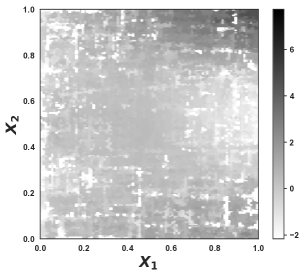
(a) Quantile Forests, $\tau=0.05$.

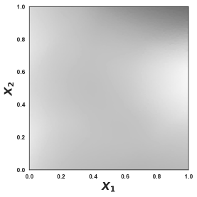
(b) Quantile Network, $\tau=0.05$.

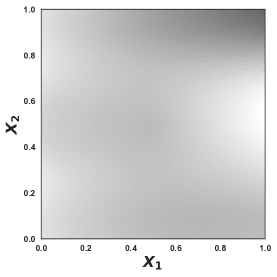
(c) True $f_{\tau}^{*}$, $\tau=0.05$.

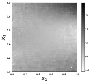
(d) Quantile Forests, $\tau=0.50$.

(e) Quantile Network, $\tau=0.50$.

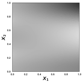
(f) True $f_{\tau}^{*}$, $\tau=0.50$.

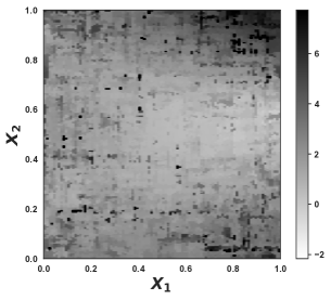
(g) Quantile Forests, $\tau=0.95$.

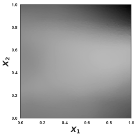
(h) Quantile Network, $\tau=0.95$.

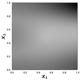
(i) True $f_{\tau}^{*}$, $\tau=0.95$.

Figure 1: One instance of the true quantile function with $\tau\in\{0.05,0.50,0.95\}$ and its corresponding estimates based on Quantile Network and Quantile Forests. Here $n=10000$ and the data are generated under Scenario 1.

Scenario 5.

The function $f_{0}\,:\,[0,1]^{10}\rightarrow\mathbb{R}$ is defined as $f_{0}(q)=g_{3}\circ g_{2}\circ g_{1}(q)$ where

$$\begin{array}[]{lll}g_{1}(q)&=&(\sqrt{q_{1}^{2}+\sum_{j=2}^{10}q_{j}},(\sum_{j=1}^{10}q_{j})^{3})^{\top},\,\,q\in[0,1]^{10},\\ g_{2}(q)&=&(|q_{1}|,q_{2}\cdot q_{1})^{\top},\,\,q\in[0,1]^{2},\\ g_{3}(q)&=&q_{1}+\sqrt{q_{1}+q_{2}},\,\,q\in[0,1]^{2},\\ \end{array}$$

where $\epsilon_{i}\overset{\text{ind}}{\sim}t(3)$ for $i=1,\ldots,n$, and $t(3)$ denotes the $t$-distribution with $3$ degrees of freedom.

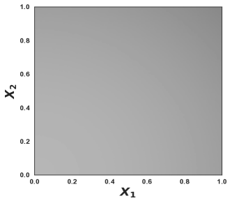
(a) $f_{\tau}^{*}$

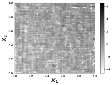
(b) Quantile Forests

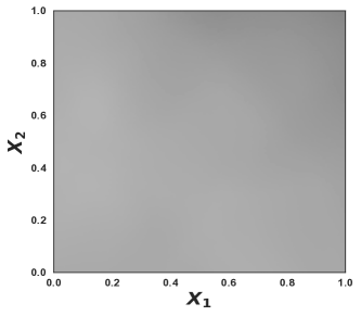
(c) Quantile Network

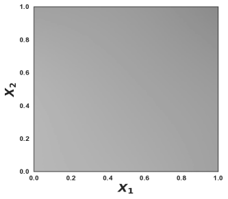
(d) Quantile Spline

Figure 2: One instance of the true quantile function with $\tau=0.25$ and its corresponding estimates obtained from different methods. Here $n=10000$ and the data are generated under Scenario 2.

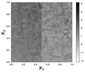
(a) Quantile Forests, $\tau=0.50$

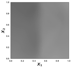
(b) Quantile Network, $\tau=0.50$

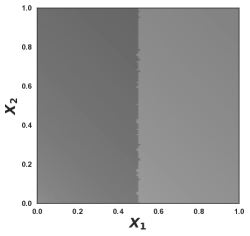
(c) True $f_{\tau}^{*}$, $\tau=0.50$

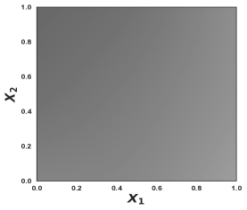
(d) Quantile Spline, $\tau=0.50$

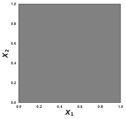
(e) SqErr Network, $\tau=0.50$

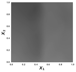
(f) Quantile Network, $\tau=0.75$

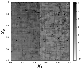
(g) Quantile Forests, $\tau=0.75$.

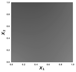
(h) Quantile Spline, $\tau=0.75$.

(i) True $f_{\tau}^{*}$, $\tau=0.75$

Figure 3: One instance of the true quantile function with $\tau\in\{0.50,0.75\}$ and of the corresponding estimates obtained with the different methods. Here $n=10000$ and the data are generated under Scenario 3.

Scenario 1
$n$	Method	$\tau=0.05$	$\tau=0.25$	$\tau=0.50$	$\tau=0.75$	$\tau=0.95$
$100$	SqErr Network	*	*	0.98	*	*
	Quantile Network	0.60	0.50	0.46	0.68	1.85
	Quantile Spline	1.79	0.19	0.14	0.17	3.36
	Quantile Forests	1.69	0.54	0.34	0.69	2.37
$1000$	SqErr Network	*	*	0.95	*	*
	Quantile Network	0.36	0.06	0.04	0.06	0.18
	Quantile Spline	0.17	0.07	0.06	0.07	0.17
	Quantile Forests	1.76	0.20	0.07	0.22	1.77
$10000$	SqErr Network	*	*	0.94	*	*
	Quantile Network	0.04	0.01	0.01	0.01	0.03
	Quantile Spline	0.07	0.06	0.06	0.06	0.07
	Quantile Forests	2.90	0.16	0.08	0.67	13.89
Scenario 2
$n$	Method	$\tau=0.05$	$\tau=0.25$	$\tau=0.50$	$\tau=0.75$	$\tau=0.95$
$100$	SqErr Network	*	*	0.28	*	*
	Quantile Network	3.82	2.37	2.21	2.64	4.43
	Quantile Spline	5.51	1.28	0.75	1.28	7.27
	Quantile Forests	4.13	1.68	1.10	1.66	4.42
$1000$	SqErr Network	*	*	0.26	*	*
	Quantile Network	0.41	0.23	0.21	0.24	0.48
	Quantile Spline	0.72	0.11	0.04	0.11	0.53
	Quantile Forests	4.08	1.24	0.68	1.18	3.62
$10000$	SqErr Network	*	*	0.19	*	*
	Quantile Network	0.07	0.03	0.03	0.04	0.08
	Quantile Spline	0.06	0.01	0.00	0.01	0.06
	Quantile Forests	3.47	1.03	0.56	1.04	3.55
Scenario 3
$n$	Method	$\tau=0.05$	$\tau=0.25$	$\tau=0.50$	$\tau=0.75$	$\tau=0.95$
$100$	SqErr Network	*	*	0.24	*	*
	Quantile Network	1.33	0.80	0.93	1.57	2.83
	Quantile Spline	6.87	0.39	0.30	0.43	4.75
	Quantile Forests	5.49	0.81	0.37	0.81	4.42
$1000$	SqErr Network	*	*	0.25	*	*
	Quantile Network	0.21	0.09	0.08	0.09	0.32
	Quantile Spline	0.50	0.10	0.08	0.09	0.53
	Quantile Forests	11.26	0.93	0.20	0.77	9.96
$10000$	SqErr Network	*	*	0.17	*	*
	Quantile Network	0.05	0.03	0.03	0.03	0.07
	Quantile Spline	0.09	0.07	0.07	0.07	0.11
	Quantile Forests	17.75	0.67	0.15	0.49	12.48

Table 1: Univariate Responses Tasks. Performances of different methods in Scenarios 1 – 3, in terms of squared error from the true quantile averaged over 25 independent trials.

Scenario 4
n	Method	$\tau=0.05$	$\tau=0.25$	$\tau=0.50$	$\tau=0.75$	$\tau=0.95$
$100$	SqErr Network	*	*	0.30	*	*
	Quantile Network	5.96	3.06	3.44	4.02	5.13
	Quantile Spline	*	*	*	*	*
	Quantile Forests	3.65	1.85	1.11	1.60	3.55
$1000$	SqErr Network	*	*	0.13	*	*
	Quantile Network	1.09	0.54	0.44	0.58	1.33
	Quantile Spline	*	*	*	*	*
	Quantile Forest	2.53	0.76	0.37	0.82	2.69
$10000$	SqErr Network	*	*	0.05	*	*
	Quantile Network	0.20	0.09	0.07	0.10	0.25
	Quantile Spline	*	*	*	*	*
	Quantile Forest	1.71	0.42	0.18	0.42	1.71
Scenario 5
$n$	Model	$\tau=0.05$	$\tau=0.25$	$\tau=0.50$	$\tau=0.75$	$\tau=0.95$
$100$	SqErr Network	*	*	30.59	*	*
	Quantile Network	5.05	4.37	3.61	4.26	6.96
	Quantile Spline	*	*	*	*	*
	Quantile Forest	41.86	21.94	15.36	20.69	53.68
$1000$	SqErr Network	37.42	31.85	30.97	31.26	35.60
	Quantile Network	1.61	1.15	0.65	0.95	2.05
	Quantile Spline	*	*	*	*	*
	Quantile Forest	29.01	12.53	7.33	11.05	33.29
$10000$	SqErr Network	35.97	31.13	30.60	31.24	36.31
	Quantile Network	0.28	0.22	0.17	0.24	0.39
	Quantile Spline	*	*	*	*	*
	Quantile Forest	17.28	7.03	3.70	5.77	18.50

Table 2: Univariate Responses Tasks: Performance of different methods in Scenarios 4 and 5, in terms of squared error from the true quantile averaged over 25 independent trials.

We visualize the performances different approaches and true quantile functions in Figures 2–3. There, we can see that Quantile Network is a better estimate for the quantile functions in general, compared to the other methods.

We report the results for Scenarios 1-3 in Table 1 and Scenarios 4-5 in Table 2. From Table 1 we can see that in Scenario 1, the Quantile Network method outperforms the competitors for most quantiles and sample sizes. The advantage becomes more evident as the sample size grows. The closest competitor is Quantile Spline which is the best method in some small sample problems. Furthermore, in Scenario 2 the best method is Quantile Spline, with Quantile Network as second best. This is not surprising since Scenario 2 consists of very smooth quantile functions defined in a low dimensional domain ($d=2$). In contrast, Scenario 3 consists of a quantile function with discontinuities and heteroscedastic errors. In this more challenging setting, Quantile Network outperforms others for larger values of $n$.

We do not compare against Quantile Splines in Scenarios 4–5 as such method does not scale up to 5 dimensional problems or above. In Table 2, we show that for Scenarios 4–5 the clear best method is Quantile Network (for $n>100$), with Quantile Forests as the second best.

Overall, the results in Tables 1-2 demonstrate a clear advantage of the Quantile Network method. This method generally outperforms SqErr Network in all examples, presumably due to the heavy-tailed or heteroscedastic error distributions. At the same time, Quantile Network also outperforms the other competitors with larger sample size or more complicated quantile functions.

4.2 Multivariate response

We explore the performance of different quantile ReLU network approaches for multivariate responses as discussed in Section 2.2. We refer to the estimator in equation (6) as Geometric Quantile, and the estimator in equation (9) as Quantile Network. As a benchmark, once again, we consider the estimator based on the squared error loss and as defined in equation (7). For all these estimators, the corresponding network class is chosen as in section 4.1.

We conduct simulations in two different scenarios. In each scenario, we evaluate performance based on mean squared error defined as

$$\frac{1}{np}\sum_{j=1}^{p}\sum_{i=1}^{n}\left(f_{\tau,j}^{*}(x_{i})-\hat{f}(x_{i})\right)^{2},$$

where the quantile functions $f_{\tau,j}^{*}(\cdot)$, $j=1,\ldots,p$, are defined in (8), and $\tau=0.5$.

We consider two multivariate response generative models as the follows.

Scenario 6.

$$\begin{array}[]{lll}y_{i}&=&g_{2}\circ g_{1}(x_{i})+\epsilon_{i}\\ g_{1}(q)&=&(|q_{1}|,q_{2}\cdot q_{1})^{\top}\\ g_{2}(q)&=&(\sqrt{q_{2}^{2}+q_{1}},(q_{1}+q_{2})^{3})^{\top}\\ x_{i}&\overset{\text{ind}}{\sim}&U[0,1]^{2},\,\,\,i=1,\ldots,n,\\ \epsilon_{i}&\overset{\text{ind}}{\sim}&Mt_{3}(0,I_{2}),\,\,\,i=1,\ldots,n,\end{array}$$

where $Mt_{3}(0,I_{2})$ is the multivariate $t$-distribution with $3$ degrees of freedom and scale matrix identity $I_{2}\in\mathbb{R}^{2\times 2}$.

Scenario 7.

$$\begin{array}[]{lll}y_{i}&=&f_{0}(x_{i})+\epsilon_{i}\\ f_{0}(q)&=&(\sqrt{q_{1}^{2}+q_{2}^{2}},\sqrt{q_{3}^{2}+q_{4}^{2}})^{\top}\\ x_{i}&\overset{\text{ind}}{\sim}&U[0,1]^{4},\\ \epsilon_{i,j}&\overset{\text{ind}}{\sim}&\mathrm{Laplace}(0,2).\end{array}$$

Scenario 6
n	Method	$\tau=0.50$
$100$	SqErr Network	0.92
	Quantile Network	0.49
	Geometric Quantile	0.54
$1000$	SqErr Network	0.91
	Quantile Network	0.06
	Geometric Quantile	0.07
$10000$	SqErr Network	0.89
	Quantile Network	0.01
	Geometric Quantile	0.01
Scenario 7
n	Method	$\tau=0.50$
$100$	SqErr Network	0.24
	Quantile Network	1.67
	Geometric Quantile	2.36
$1000$	SqErr Network	0.11
	Quantile Network	0.23
	Geometric Quantile	0.14
$10000$	SqErr Network	0.09
	Quantile Network	0.03
	Geometric Quantile	0.03

Table 3: Multivariate Responses Tasks: Performance of different methods in Scenarios 6 and 7.

Note: We measure performance using the averaged mean squared error based on 25 Monte Carlo simulations for the two synthetic multivariate benchmarks.

Table 3 illustrates the performance of different methods in Scenarios 6 and 7 with sample sizes $n=\{100,1000,10000\}$. We can see that both Quantile Network and Geometric Quantile outperform the $\ell_{2}$-based approach SqErr Network. This corroborates the results earlier in Section 4.1. Particularly, it demonstrates that both Quantile Network and Geometric Quantile are robust estimators when dealing with heavy-tailed distributions.

5 Conclusion and Future Work

In this paper we have studied, both theoretically and empirically, the statistical performance of ReLU networks for quantile regression. Our main theorems establish minimax estimation rates under general classes of functions and distributions of the errors. These results rely on the approximation theory from Schmidt-Hieber (2017) and Suzuki (2018). Future work can extend these results to other function classes provided that the corresponding approximation theory is used or developed. Empirically, experiments in both univariate and multivariate response quantile regression with ReLU networks show an advantage over other quantile regression methods. Quantile regression networks were also shown to outperform $\ell_{2}$-based regression with the same neural network architecture when the error distribution is heavy-tailed. In the case of multivariate responses, quantile networks were also shown to perform well in benchmarks. A theoretical study of statistical rates of convergence for multivariate response neural quantile regression is left for future work.

Appendix A Notation

For an $\epsilon>0$ and a metric $\mathrm{dist}(\cdot,\cdot)$ on the class of functions $\mathcal{F}$, we define the covering number $\mathrm{N}(\epsilon,\mathcal{F},\mathrm{dist}(\cdot,\cdot))$ as the minimum number of balls of the form $\{g\,:\,\mathrm{dist}(g,f)\leq\epsilon\}$, with $f\in\mathcal{F}$, needed to cover $\mathcal{F}$.

We also write

$$\text{B}(f,\|\cdot\|_{\ell_{2}},r)\,=\,\,\{g\,:\,\|f-g\|_{\ell_{2}}\leq r\}.$$

Furrthermore, if $a_{n}$ and $b_{n}$ are positive sequences, we say that $a_{n}\lesssim b_{n}$ if there exists $m$ such that $n\geq m$ implies $a_{n}\leq cb_{n}$ for a constant $c>0$.

Appendix B Theorem 1

Througouth this section we write $\mathcal{F}$ to refer to $\mathcal{F}(W,U,L)$.

B.1 Auxiliary results

Before stating our first result we first state some definitions and an auxiliary lemma.

Definition 6.

We define the empirical loss function

$$\hat{M}_{n}(\theta)=\sum_{i=1}^{n}\hat{M}_{n,i}(\theta),$$

where

$$\hat{M}_{n,i}(f)=\frac{1}{n}\left(\rho_{\tau}(y_{i}-f(x_{i}))-\rho_{\tau}(y_{i}-f_{n}(x_{i}))\right),$$

with

$$f_{n}\,\in\,\underset{f\in\mathcal{F}}{\arg\min}\,\,\,\mathbb{E}\left[\frac{1}{n}\sum_{i=1}^{n}\rho_{\tau}(y_{i}-f(x_{i}))-\frac{1}{n}\sum_{i=1}^{n}\rho_{\tau}(y_{i}-f_{\tau}^{*}(x_{i}))\right].$$

We also set

$$M_{n,i}(f)=\frac{1}{n}\mathbb{E}[\rho_{\tau}(z_{i}-f(x_{i}))-\rho_{\tau}(z_{i}-f_{n}(x_{i}))],$$

where $z\in\mathbb{R}^{n}$ is an independent copy of $y$.

Lemma 4.

Suppose that Assumption 1–2 hold. Then there exists a constant $c_{\tau}$ such that for all $\delta\in\mathbb{R}^{n}$, we have

$$\sum_{i=1}^{n}\mathbb{E}\left[\rho_{\tau}(z_{i}-f_{\tau}^{*}(x_{i})-\delta_{i})\right]-\sum_{i=1}^{n}\mathbb{E}\left[\rho_{\tau}(z_{i}-f_{\tau}^{*}(x_{i}))\right]\geq c_{\tau}n\Delta_{n}^{2}(\delta),$$

where $z\in\mathbb{R}^{n}$ is an independent copy of $y$.

Proof.

See Lemma 8 in Padilla and Chatterjee (2020). ∎

Definition 7.

Let $\mathcal{H}$ be a class of functions from $\mathcal{X}$ to $\mathbb{R}$. We define the pseudodimension of $\mathcal{H}$, denoted as $\mathrm{Pdim}(\mathcal{H})$, as the largest integer $m$ for which there exist $(a_{1},b_{1})\ldots,(a_{m},b_{m})\in\mathcal{X}\times\mathbb{R}$ such that for all $\eta\in\{0,1\}^{m}$ there exists $f\in\mathcal{H}$ such that

$$f(a_{i})>b_{i}\,\,\,\,\iff\,\,\,\,\eta_{i},$$

for $i=1,\ldots,m$.

Theorem 5 (Theorem 7 from Bartlett et al. (2019)).

With the notation from before, we have that

$$\mathrm{Pdim}\left(\mathcal{F}(W,U,L)\right)=O(LW\log(U)).$$

B.2 Proof of Theorem 1

Proof.

Throughout this proof the covariates $x_{1},\ldots,x_{n}$ are fixed. Let $\hat{\delta}_{i}=\hat{f}(x_{i})-f_{\tau}^{*}(x_{i})$ for $i=1,\ldots,n$. Notice that

$$\begin{array}[]{lll}\displaystyle\mathbb{E}\left[\frac{1}{n}\sum_{i=1}^{n}D^{2}\left\{f_{\tau}^{*}(x_{i})-\hat{f}(x_{i})\right\}\right]&\leq&\displaystyle\frac{1}{c_{\tau}n}\mathbb{E}\left(\sum_{i=1}^{n}\mathbb{E}\left[\rho_{\tau}\{z_{i}-f_{\tau}^{*}(x_{i})-\hat{\delta}_{i}\}\right]-\sum_{i=1}^{n}\mathbb{E}\left[\rho_{\tau}\{z_{i}-f_{\tau}^{*}(x_{i})\}\right]\right)\\ &=&\displaystyle\frac{1}{c_{\tau}}E\left\{M_{n}(\hat{f})\right\}+\frac{1}{c_{\tau}}\text{err}_{1},\end{array}$$ (17)

where the inequality follows from Lemma 4.

Next we proceed to bound $E\{M_{n}(\hat{f})\}$. To that end, notice that for a constant $C>0$,

$$\begin{array}[]{lll}\mathbb{E}\left\{M_{n}(\hat{f})\right\}&\leq&\displaystyle 4\mathbb{E}\left\{\underset{f\in\mathcal{F}}{\sup}\,\frac{1}{n}\sum_{i=1}^{n}\xi_{i}f(x_{i})\right\}\\ &\leq&\displaystyle F\mathbb{E}\left\{\underset{f\in\mathcal{F}}{\sup}\,\frac{1}{n}\sum_{i=1}^{n}\xi_{i}\frac{f(x_{i})}{F}\right\}\\ &\leq&\displaystyle\frac{CF}{\sqrt{n}}\,\int_{0}^{2}\sqrt{\log\mathrm{N}\left(\mu,\mathcal{F}/F,\|\cdot\|_{n}\right)}\,d\mu\\ &\leq&\displaystyle\frac{CF}{\sqrt{n}}\,\int_{0}^{2}\sqrt{\log\left(\left(\frac{2\cdot e\cdot n}{\mu\cdot\mathrm{Pdim}\left(\mathcal{F}\right)}\right)^{\mathrm{Pdim}\left(\mathcal{F}\right)}\right)}\,d\mu\\ &\leq&\displaystyle\tilde{C}F\sqrt{\frac{LW\log U\cdot\log n}{n}}\end{array}$$

for some constant $\tilde{C}>0$, where the first inequality follows by simmetrization and Talgrand’s inequality (Ledoux and Talagrand (2013)) similarly to Theorem 12 in Padilla and Chatterjee (2020), the third inequality follows from Dudley’s theorem, the fourth holds because of Lemma 4 in Farrell et al. (2018), and the last from Theorem 5.

∎

Appendix C Theorem 3

The proof is in the spirit of the proof of Theorem 1 in Farrell et al. (2018) combined with results and ideas from Padilla and Chatterjee (2020) and Suzuki (2018).

C.1 Notation

Througout we let $\mathcal{X}=[0,1]^{d}$. For $p>0$ and $f\,:\,\mathcal{X}\,\rightarrow\,\mathbb{R}$ we let

$$\|f\|_{p}\,:=\,\left(\int_{\mathcal{X}}(f(x))^{p}dx\right)^{1/p}$$

and

$$L^{p}(\mathcal{X})\,=\,\left\{f\,:\,f\,:\,\mathcal{X}\,\rightarrow\,\mathbb{R},\,\,\,\,\text{and}\,\,\,\,\|f\|_{p}<\infty\right\}.$$

Definition 8.

For a function $f\in L^{p}(\mathcal{X})$ and $p\in(0,\infty]$ we define the $r$-modulus of continuity as

$$w_{r,p}(f,t)=\underset{\|h\|_{2}\leq t}{\sup}\,\|\Delta_{h}^{r}(f)\|_{p},$$

with

$$\Delta_{h}^{r}(f)=\begin{cases}\sum_{j=0}^{r}\frac{r!}{j!\,(j-r)!}(-1)^{r-j}f(x+hj)&\text{if}\,\,\,\,\,x\in\mathcal{X},\,\,\,x+rh\in\mathcal{X},\\ 0&\text{otherwise}.\end{cases}$$

Definition 9.

For $0<p,q\leq\infty$, $\alpha>0$, $r=\lfloor\alpha\rfloor+1$, we define the Besov space $B^{\alpha}_{p,q}(\mathcal{X})$ as

$$B^{\alpha}_{p,q}(\mathcal{X})=\left\{f\in L^{p}(\mathcal{X})\,:\,\|f\|_{B^{\alpha}_{p,q}(\mathcal{X})}<\infty\right\},$$

where

$$\|f\|_{B^{\alpha}_{p,q}(\mathcal{X})}=\|f\|_{p}+|f|_{B^{\alpha}_{p,q}(\mathcal{X})},$$

with

$$|f|_{B^{\alpha}_{p,q}(\mathcal{X})}=\begin{cases}\left(\int_{0}^{\infty}(t^{-\alpha}w_{r,p}(f,t))^{q}t^{-1}dt\right)^{\frac{1}{q}}&\,\,\,\text{if }\,\,\,\,q<\infty,\\ \underset{t>0}{\sup}\,\,\,t^{-\alpha}w_{r,p}(f,t)&\,\,\,\text{if }\,\,\,\,q=\infty.\end{cases}$$

Throughout we denote by $f_{n}\in\mathcal{I}(L,W,S,B)$ a function satisfying

$$f_{n}\in\underset{f\in\mathcal{I}(L,W,S,B),\,\|f\|_{\infty}\leq F}{\arg\min}\,\|f-f_{\tau}^{*}\|_{\infty}.$$

We also write

$$\tilde{\mathcal{I}}(L,W,S,B)=\left\{f\in\mathcal{I}(L,W,S,B)\,:\,\,\|f\|_{\infty}\leq F\right\}.$$

C.2 Auxiliary lemmas

Lemma 6.

Suppose that $\|f_{n}-f_{\tau}^{*}\|_{\infty}\leq c$ for a small enough constant $c$. With the notation in (11) we have that

$$\Delta^{2}(f,f_{n})\leq\frac{1}{c_{\tau}}\left[\mathbb{E}\left(\rho_{\tau}(Y-f(X))-\rho_{\tau}(Y-f_{n}(X))\right)+\|f_{n}-f_{\tau}^{*}\|_{\infty}\Delta(f,f_{n})\sqrt{F}\right],$$

and

$$\|f-f_{n}\|_{\ell_{2}}^{2}\leq\frac{2F}{c_{\tau}}\left[\mathbb{E}\left(\rho_{\tau}(Y-f(X))-\rho_{\tau}(Y-f_{n}(X))\right)+\|f_{n}-f_{\tau}^{*}\|_{\infty}\|f-f_{n}\|_{\ell_{2}}\sqrt{F}\right],$$

for any $f\in\tilde{\mathcal{I}}(L,W,S,B)$ and for some constant $c_{\tau}$.

Proof.

Notice that by Equation B.3 in Belloni and Chernozhukov (2011),

$$\begin{array}[]{lll}\rho_{\tau}(Y-f(X))-\rho_{\tau}(Y-f_{n}(X))&=&\displaystyle-(f(X)-f_{n}(X))(\tau-1{\{Y\leq f_{n}(X)\}})+\\ &&\displaystyle\int_{0}^{f(X)-f_{n}(X)}\left[1\{Y\leq f_{n}(X)+z\}-1{\{Y\leq f_{n}(X)\}}\right]dz\\ &=&\displaystyle-(f(X)-f_{n}(X))(\tau-1{\{Y\leq f_{\tau}^{*}(X)\}})-\\ &&\displaystyle(f(X)-f_{n}(X))(1{\{Y\leq f_{\tau}^{*}(X)\}}-1{\{Y\leq f_{n}(X)\}})+\\ &&\displaystyle\int_{0}^{f(X)-f_{n}(X)}\left[1\{Y\leq f_{n}(X)+z\}-1{\{Y\leq f_{n}(X)\}}\right]dz.\\ \end{array}$$

Hence, taking expectations and using Fubini’s theorem,

$$\begin{array}[]{lll}\mathbb{E}\left(\rho_{\tau}(Y-f(X))-\rho_{\tau}(Y-f_{n}(X))\right)&=&\displaystyle\mathbb{E}\left(-(f(X)-f_{n}(X))\mathbb{E}\left((\tau-1{\{Y\leq f_{\tau}^{*}(X)\}})\bigg{|}X\right)\right)-\\ &&\displaystyle\mathbb{E}\left((f(X)-f_{n}(X))\mathbb{E}\left((1{\{Y\leq f_{\tau}^{*}(X)\}}-1{\{Y\leq f_{n}(X)\}})\bigg{|}X\right)\right)+\\ &&\displaystyle\mathbb{E}\bigg{(}\int_{0}^{f(X)-f_{n}(X)}\bigg{[}\mathbb{E}\left(1\{Y\leq f_{n}(X)+z\}\bigg{|}X\right)-\\ &&\,\,\,\,\,\,\,\,\,\mathbb{E}\left(1\{Y\leq f_{n}(X)\}\bigg{|}X\right)\bigg{]}dz\bigg{)}\\ &\geq&-c_{1}\mathbb{E}\left[|f(X)-f_{n}(X)|\cdot|f_{\tau}^{*}(X)-f_{n}(X)|\right]+\\ &&c_{\tau}\mathbb{E}(D^{2}(f(X)-f_{n}(X)))\\ &\geq&-c_{1}\sqrt{\mathbb{E}\left[|f(X)-f_{n}(X)|^{2}\right]}\sqrt{\mathbb{E}\left[|f_{\tau}^{*}(X)-f_{n}(X)|^{2}\right]}+\\ &&c_{\tau}\mathbb{E}(D^{2}(f(X)-f_{n}(X)))\\ &\geq&-c_{1}\|f_{n}-f_{\tau}^{*}\|_{\infty}\sqrt{F\Delta^{2}(f,f_{n})}\\ &&c_{\tau}\mathbb{E}(D^{2}(f(X)-f_{n}(X)))\\ \end{array}$$

for a constant $c_{1}>0$, where the first inequality holds since the cumulative distribution function of $Y$ conditioning on $X$ is Lipchitz around $f_{\tau}^{*}(X)$ by Assumption 2, and by the same argument from the proof of Lemma 8 in Padilla and Chatterjee (2020).

∎

Definition 10.

We define the empirical loss function

$$\hat{M}_{n}(\theta)=\sum_{i=1}^{n}\hat{M}_{n,i}(\theta),$$

where

$$\hat{M}_{n,i}(f)=\frac{1}{n}\left[\rho_{\tau}\{y_{i}-f(x_{i})\}-\rho_{\tau}\{y_{i}-f_{n}(x_{i})\}\right],$$

and we set

$$M_{n}(f)=\mathbb{E}[\rho_{\tau}\{Y-f(X)\}-\rho_{\tau}\{Y-f_{n}(X)\}].$$

Lemma 7.

Suppose that $\|f_{n}-f_{\tau}^{*}\|_{\infty}\leq c$ for a small enough constant $c$. The estimator $\hat{f}$ defined in (16) satisfies

$$\Delta^{2}(\hat{f},f_{n})\leq\frac{1}{c_{\tau}}\left[M_{n}(\hat{f})-\hat{M}_{n}(\hat{f})+\|f_{n}-f_{\tau}^{*}\|_{\infty}\Delta(\hat{f},f_{n})\sqrt{F}\right].$$

Furthermore,

$$\|\hat{f}-f_{n}\|_{\ell_{2}}^{2}\leq\frac{2F}{c_{\tau}}\left[M_{n}(\hat{f})-\hat{M}_{n}(\hat{f})+\|f_{n}-f_{\tau}^{*}\|_{\infty}\|\hat{f}-f_{n}\|_{\ell_{2}}\sqrt{F}\right].$$

Proof.

By Lemma 6 we have that

$$\begin{array}[]{lll}\Delta^{2}(\hat{f},f_{n})&\leq&\displaystyle\frac{1}{c_{\tau}}\left[\mathbb{E}\left(\rho_{\tau}(Y-\hat{f}(X))-\rho_{\tau}(Y-f_{n}(X))\right)+\|f_{n}-f_{\tau}^{*}\|_{\infty}\Delta(\hat{f},f_{n})\sqrt{F}\right]\\ &\leq&\displaystyle\frac{1}{c_{\tau}}\bigg{[}\mathbb{E}\left(\rho_{\tau}(Y-\hat{f}(X))-\rho_{\tau}(Y-f_{n}(X))\right)+\|f_{n}-f_{\tau}^{*}\|_{\infty}\Delta(\hat{f},f_{n})\sqrt{F}-\\ &&\displaystyle\frac{1}{n}\sum_{i=1}^{n}\rho_{\tau}(y_{i}-\hat{f}(x_{i}))+\sum_{i=1}^{n}\rho_{\tau}(y_{i}-f_{n}(x_{i}))\bigg{]},\end{array}$$

where the last inequality follows by the optimality of $\hat{f}$. ∎

Lemma 8.

Suppose that

$$3\mathbb{E}\left(\underset{f\in\tilde{\mathcal{I}}(L,W,S,B),\,\,\|f-f_{n}\|^{2}_{\ell_{2}}\leq r^{2}}{\sup}\,\frac{1}{n}\sum_{i=1}^{n}\xi_{i}(f(x_{i})-f_{n}(x_{i}))^{2}\right)\leq r^{2},$$ (18)

for $\{\xi_{i}\}_{i=1}^{n}$ Rademacher variables independent of $\{(x_{i},y_{i})\}_{i=1}^{n}$, and

$$\max\left\{4F\sqrt{\frac{\gamma}{n}},4F\sqrt{\frac{\gamma}{3n}}\right\}\leq r.$$ (19)

Then with probability at least $1-e^{-\gamma}$, $\|f-f_{n}\|_{\ell_{2}}^{2}\leq r^{2}$ with $f\in\tilde{\mathcal{I}}(L,W,S,B)$ implies

$$\|f-f_{n}\|_{n}^{2}\,\leq\,(2r)^{2}.$$

Proof.

First notice that

$$|(f(x)-f_{n}(x))^{2}|\leq 2\left[F^{2}+\|f_{n}\|_{\infty}^{2}\right],$$

for all $x$. Hence,

$$\begin{array}[]{lll}\mathbb{E}\left(\left(f(X)-f_{n}(X)\right)^{4}\right)&\leq&2(F^{2}+\|f_{n}\|_{\infty}^{2})\mathbb{E}\left(\left(f(X)-f_{n}(X)\right)^{2}\right)\\ &\leq&4F^{2}\|f-f_{n}\|_{\ell_{2}}^{2}\end{array}$$

Then by Theorem 2.1 in Bartlett et al. (2005) with probability at least $1-\exp(-\gamma)$,

$$\begin{array}[]{l}\underset{f\in\tilde{\mathcal{I}}(L,W,S,B),\,\,\|f-f_{n}\|_{\ell_{2}}^{2}\leq r^{2}}{\sup}\,\left\{\|f-f_{n}\|_{n}^{2}-\|f-f_{n}\|_{\ell_{2}}^{2}\right\}\\ \leq\displaystyle 3\mathbb{E}\left(\underset{f\in\tilde{\mathcal{I}}(L,W,S,B),\,\,\|f-f_{n}\|_{\ell_{2}}^{2}\leq r^{2}}{\sup}\,\frac{1}{n}\sum_{i=1}^{n}\xi_{i}(f(X_{i})-f_{n}(X_{i}))^{2}\right)\\ \displaystyle+4rF\sqrt{\frac{\gamma}{n}}+\frac{16F^{2}\gamma}{3n}\\ \end{array}$$ (20)

and the claim follows. ∎

Lemma 9.

Suppose that $\|\hat{f}-f_{n}\|_{\ell_{2}}\leq r_{0}$, with $r_{0}$ satisfying (18)-(19) and Assumption 5 holds. Also, with the notation of Assumption 4, suppose that for the class $\mathcal{I}(L,W,S,B)$ the parameters are chosen as

$$\begin{array}[]{l}L=3+2\lceil\log_{2}\left(\frac{3^{\max\{d,m\}}}{\epsilon c_{d,m}}\right)+5\rceil\lceil\log_{2}\max\{d,m\}\rceil,\,\,\,\,\,\,\,W=W_{0}N,\\ S=(L-1)W_{0}^{2}N+N,\,\,\,\,\,\,B=O\left(N^{(v^{-1}+d^{-1})(\max\{1,(d/p-s)_{+}\})}\right),\end{array}$$

for a constant $c_{d,m}$ that depends on $d$ and $m$, a constant $W_{0}$, and where $v=(s-\delta)/\delta$,

$$\delta=\frac{d}{p},\,\,\,\,\,\,\,\,\,\,\,\,\,\,N\asymp n^{\frac{d}{2s+d}}.$$

Then for some positive constant $C_{0}$ it holds that

$$\begin{array}[]{lll}\,\|\hat{f}-f_{n}\|^{2}_{\ell_{2}}&\leq&C_{0}\bigg{[}r_{0}F^{2.5}\sqrt{\frac{\gamma}{n}}+\frac{F^{2.5}\gamma}{n}+\\ &&r_{0}F\sqrt{\frac{N(\log N)^{2}}{n}}+r_{0}F\sqrt{\frac{N\left[(\log N)^{2}+\log r_{0}^{-1}+\log n\right]}{n}}+N^{-s/d}r_{0}F^{1.5}\bigg{]}\end{array}$$

with probability at least $1-\exp(-\gamma)$, where $N\asymp n^{\frac{d}{2s+d}}$.

Proof.

Let

$$\mathcal{G}=\left\{g\,:\,g(x,y)=\rho_{\tau}(y-f(x))-\rho_{\tau}(y-f_{n}(x)),\,\,\,f\in\tilde{\mathcal{I}}(L,W,S,B),\,\,\|f-f_{n}\|_{\ell_{2}}\leq r_{0}\right\}.$$

Then for $\xi_{1},\ldots,\xi_{n}$ independent Rademacher variables independent of $\{(x_{i},y_{i})\}_{i=1}^{n}$, we have that

$$\begin{array}[]{lll}c_{\tau}\,\|\hat{f}-f_{n}\|_{\ell_{2}}^{2}&\leq&2F[M_{n}(\hat{f})-\hat{M}_{n}(\hat{f})+\|f_{n}-f_{\tau}^{*}\|_{\infty}\|\hat{f}-f_{n}\|_{\ell_{2}}\sqrt{F}]\\ &\leq&\displaystyle 2F\underset{g\in\mathcal{G}}{\sup}\left\{\mathbb{E}(g(X,Y))-\frac{1}{n}\sum_{i=1}^{n}g(x_{i},y_{i})\right\}+\|f_{n}-f_{\tau}^{*}\|_{\infty}\|\hat{f}-f_{n}\|_{\ell_{2}}F^{3/2}\\ &\leq&\displaystyle 12F\mathbb{E}\left(\underset{g\in\mathcal{G}}{\sup}\,\frac{1}{n}\sum_{i=1}^{n}\xi_{i}g(x_{i},y_{i})\bigg{|}(x_{1},y_{1}),\ldots,(x_{n},y_{n})\right)\\ &&\displaystyle+4r_{0}F^{2.5}\sqrt{\frac{\gamma}{n}}+\frac{100F^{2.5}\gamma}{3n}+\|f_{n}-f_{\tau}^{*}\|_{\infty}\|\hat{f}-f_{n}\|_{\ell_{2}}F^{1.5},\\ \end{array}\,$$ (21)

where the first inequality follows from Lemmas 7, and the third happens with probability at least $1-e^{-\gamma}$ and holds by Theorem 2.1 in Bartlett et al. (2005).

Next, notice that for a constant $C>0$,

$$\begin{array}[]{lll}\displaystyle\mathbb{E}_{\xi}\left(\underset{g\in\mathcal{G}}{\sup}\,\frac{1}{n}\sum_{i=1}^{n}\xi_{i}g(x_{i},y_{i})\right)&\leq&\displaystyle\mathbb{E}_{\xi}\left(\underset{f\in\mathcal{I}(L,W,S,B),\,\,\|f\|_{\infty}\leq F\,\,\|f-f_{n}\|_{\ell_{2}}\leq r_{0}}{\sup}\,\frac{1}{n}\sum_{i=1}^{n}\xi_{i}(f(x_{i})-f_{n}(x_{i}))\right)\\ &\leq&\displaystyle\mathbb{E}_{\xi}\left(\underset{f\in\mathcal{I}(L,W,S,B),\,\,\|f\|_{\infty}\leq F,\,\,\|f_{n}-f\|_{n}\leq 2r_{0}}{\sup}\,\frac{1}{n}\sum_{i=1}^{n}\xi_{i}(f(x_{i})-f_{n}(x_{i}))\right)\\ &\leq&\displaystyle\underset{0<\alpha<2r_{0}}{\inf}\left\{4\alpha+\frac{12}{\sqrt{n}}\int_{\alpha}^{2r_{0}}\sqrt{\log\mathcal{N}(\delta,\tilde{\mathcal{I}}(L,W,S,B),\|\cdot\|_{n})}d\delta\right\}\\ &\leq&\displaystyle\underset{0<\alpha<2r_{0}}{\inf}\left\{4\alpha+\frac{12}{\sqrt{n}}\int_{\alpha}^{2r_{0}}\sqrt{\log\mathcal{N}(\delta,\tilde{\mathcal{I}}(L,W,S,B),\|\cdot\|_{\infty})}d\delta\right\}\\ &\leq&\displaystyle\underset{0<\alpha<r_{0}}{\inf}\left\{4\alpha+\frac{24r_{0}}{\sqrt{n}}\sqrt{\log\mathcal{N}(\alpha,\tilde{\mathcal{I}}(L,W,S,B),\|\cdot\|_{\infty})}\right\},\\ &\leq&C\displaystyle\underset{0<\alpha<r_{0}}{\inf}\left\{\alpha+r_{0}\sqrt{\frac{N\left[(\log N)^{2}+\log\alpha^{-1}\right]}{n}}\right\},\\ \end{array}$$ (22)

where the first inequality follows by Talagrand’s inequality (Ledoux and Talagrand, 2013), and the second holds with probability at least $1-\exp(-\gamma)$ by Lemma 8, the third by Dudley’s chaining inequality, and the last by the proof Theorem 2 in Suzuki (2018) . The latter theorem also gives $N\asymp n^{\frac{d}{2s+d}}$, and

$$\|f_{n}-f_{\tau}^{*}\|_{\infty}\leq C_{1}N^{-s/d},$$

for some constant $C_{1}>0$. Hence, taking

$$\alpha=r_{0}\sqrt{\frac{N(\log N)^{2}}{n}},$$

(21) and (22) imply

$$\begin{array}[]{lll}\,\|\hat{f}-f_{\tau}^{*}\|_{\ell_{2}}^{2}&\leq&\frac{1}{c_{\tau}}\bigg{[}4r_{0}F^{2.5}\sqrt{\frac{\gamma}{n}}+\frac{100F^{2.5}\gamma}{3n}+\\ &&Cr_{0}F\sqrt{\frac{N(\log N)^{2}}{n}}+Cr_{0}F\sqrt{\frac{N\left[(\log N)^{2}+\log r_{0}^{-1}+\log n\right]}{n}}+C_{1}r_{0}N^{-s/d}F^{1.5}\bigg{]}\end{array}$$

with probability at least $1-2e^{-\gamma}$. ∎

Lemma 10.

Let $r^{*}$ be defined as

$$r^{*}=\inf\left\{r>0\,:\,3\mathbb{E}\left(\underset{f\in\tilde{\mathcal{I}}(L,W,S,B),\,\,\|f-f_{n}\|_{\ell_{2}}\leq s}{\sup}\,\frac{1}{n}\sum_{i=1}^{n}\xi_{i}(f(x_{i})-f_{n}(x_{i}))^{2}\right)<s^{2},\,\,\forall s\geq r\right\},$$

for $\{\xi_{i}\}_{i=1}^{n}$ Rademacher variables independent of $\{(x_{i},y_{i})\}_{i=1}^{n}$. Then under the conditions of Lemma 9,

$$r^{*}\leq\displaystyle\tilde{C}\left[\sqrt{\frac{N(\log N)^{2}}{n}}+\sqrt{\frac{N\left[(\log N)^{2}+\log n\right]}{n}}\right],$$

for a constant $\tilde{C}>0$ and with $N$ satisfying $N\asymp n^{\frac{d}{2s+d}}$.

Proof.

Consider the set

$$\mathcal{G}_{r^{*}}=\left\{f\in\tilde{\mathcal{I}}(L,W,S,B)\,:\,\|f-f_{n}\|_{\ell_{2}}^{2}\leq(r^{*})^{2}\right\},$$

and the define the event

$$E\,=\,\left\{\underset{f\in\mathcal{G}_{r^{*}}}{\sup}\|f-f_{n}\|_{n}^{2}\leq(2r^{*})^{2}\right\}.$$

If $r^{*}$ satisfies (19) with $\gamma=\log n$ then we have that $\mathbb{P}(E)\geq 1-1/n$ by Lemma 8.

Also,

$$\begin{array}[]{lll}\displaystyle(r^{*})^{2}&\leq&\displaystyle 3\mathbb{E}\left(\underset{f\in\tilde{\mathcal{I}}(L,W,S,B),\,\,\|f-f_{n}\|_{\ell_{2}}^{2}\leq(r^{*})^{2}}{\sup}\,\frac{1}{n}\sum_{i=1}^{n}\xi_{i}(f(x_{i})-f_{n}(x_{i}))^{2}\right)\\ &\leq&\displaystyle 3\mathbb{E}\left(\mathbb{E}\left(\underset{f\in\tilde{\mathcal{I}}(L,W,S,B),\,\,\|f-f_{n}\|_{n}^{2}\leq(2r^{*})^{2}}{\sup}\,\frac{1}{n}\sum_{i=1}^{n}\xi_{i}(f(x_{i})-f_{n}(x_{i}))^{2}\bigg{|}x_{1},\ldots,x_{n}\right)1_{E}\right)\,+\\ &&\displaystyle\frac{12F^{2}}{n}\\ &\leq&\displaystyle 3\mathbb{E}\left(\mathbb{E}\left(\underset{f\in\tilde{\mathcal{I}}(L,W,S,B),\,\,\|f-f_{n}\|_{n}^{2}\leq(2r^{*})^{2}}{\sup}\,\frac{1}{n}\sum_{i=1}^{n}\xi_{i}(f(x_{i})-f_{n}(x_{i}))^{2}\bigg{|}x_{1},\ldots,x_{n}\right)1_{E}\right)\,+\\ &&\displaystyle\frac{12F^{2}}{n}.\\ &&\end{array}$$ (23)

Next, let

$$\mathcal{G}=\left\{g\,:\,g(x)=(f(x)-f_{n}(x))^{2},\,\,\,\text{for some}\,\,f\in\tilde{\mathcal{I}}(L,W,S,B),\,\,\,\,\|f-f_{n}\|_{n}\leq 2r^{*}\right\}.$$

Notice that if $g_{1},g_{2}\in\mathcal{G}$ with $g_{j}=f_{j}-f_{n}$, $j=1,2$, then

$$|g_{1}(x)-g_{2}(x)|\,=\,|f_{1}(x)-f_{2}(x)|\cdot|f_{1}(x)+f_{2}(x)-2f_{n}(x)|\,\leq\,4F\|f_{1}-f_{2}\|_{\infty}.$$

Hence, combining this with (23), using Dudley’s chaining we obtain that

$$\begin{array}[]{lll}\displaystyle(r^{*})^{2}&\leq&\displaystyle 3\mathbb{E}\left(\underset{0<\alpha<2r^{*}}{\inf}\left\{4\alpha+\frac{12}{\sqrt{n}}\int_{\alpha}^{2r^{*}}\sqrt{\log\mathcal{N}(\delta,\mathcal{G},\|\cdot\|_{n})}\right\}\right)+\frac{12F}{n}\\ &\leq&\displaystyle 3\mathbb{E}\left(\underset{0<\alpha<2r^{*}}{\inf}\left\{4\alpha+\frac{12}{\sqrt{n}}\int_{\alpha}^{2r^{*}}\sqrt{\log\mathcal{N}(\delta,\mathcal{G},\|\cdot\|_{\infty})}\right\}\right)+\frac{12F}{n}\\ &\leq&C\displaystyle\underset{0<\alpha<2r^{*}}{\inf}\left\{\alpha+r^{*}\sqrt{\frac{N\left[(\log N)^{2}+\log\alpha^{-1}\right]}{n}}\right\}+\frac{12F}{n},\end{array}$$ (24)

where the last inequality follows from Theorem 2 in Suzuki (2018), and with $N$ satisfying $N\asymp n^{\frac{d}{2s+d}}$. Hence, if $r^{*}$ satisfies (19) then for a constant $\tilde{C}>0$

$$r^{*}\leq\displaystyle\tilde{C}\left[\sqrt{\frac{N(\log N)^{2}}{n}}+\sqrt{\frac{N\left[(\log N)^{2}+\log n\right]}{n}}\right],$$

which follows from (24) by taking

$$\alpha=r^{*}\sqrt{\frac{N(\log N)^{2}}{n}}.$$

The claim follows. ∎

C.3 Proof of Theorem 3

Proof.

Throughout we use the notation from the proof of Lemma 9. Then we proceed as in Farrell et al. (2018). Specifically, we divide the space $\tilde{\mathcal{I}}(L,W,S,B)$ into sets of increasing radius

$$\text{B}(f_{n},\|\cdot\|_{\ell_{2}},\overline{r}),\,\text{B}(f_{n},\|\cdot\|_{\ell_{2}},2\overline{r})\backslash\text{B}(f_{n},\|\cdot\|_{\ell_{2}},\overline{r}),\ldots,\text{B}(f_{n},\|\cdot\|_{\ell_{2}},2^{l}\overline{r})\backslash\text{B}(f_{n},\|\cdot\|_{\ell_{2}},2^{l-1}\overline{r}),$$

where

$$l=\bigg{\lfloor}\log_{2}\left(\frac{2F}{\sqrt{(\log n)/n}}\right)\bigg{\rfloor}.$$

Next, if $\overline{r}>r^{*}$, the by Lemma 8, with probability at least $1-le^{-\gamma}$, we have that

$$\|f-f_{n}\|_{\ell_{2}}^{2}\leq 2^{j}\overline{r}\,\,\,\text{implies}\,\,\,\|f-f_{n}\|_{n}^{2}\leq 2^{j+1}\overline{r}.$$

Then if for some $j\leq l$ it holds that

$$\hat{f}\in\text{B}(f_{n},\|\cdot\|_{\ell_{2}},2^{j}\overline{r})\backslash\text{B}(f_{n},\|\cdot\|_{\ell_{2}},2^{j-1}\overline{r}),$$

then by Lemma 9, with probability at least $1-4e^{-\gamma}$, we have that

$$\begin{array}[]{lll}\|\hat{f}-f_{n}\|_{\ell_{2}}^{2}&\leq&\tilde{C}\bigg{[}2^{j}\overline{r}F^{2.5}\sqrt{\frac{\gamma}{n}}+\frac{F^{2.5}\gamma}{n}+\\ &&\cdot 2^{j}\overline{r}F\sqrt{\frac{N(\log N)^{2}}{n}}+\cdot 2^{j}\overline{r}F\sqrt{\frac{N\left[(\log N)^{2}+2\log n\right]}{n}}+2^{j}\overline{r}N^{-s/d}F^{1.5}\bigg{]}\\ &\leq&2^{2j-2}\overline{r}^{2},\end{array}$$

provided that

$$\tilde{C}\left[F^{2.5}\sqrt{\frac{\gamma}{n}}+F\sqrt{\frac{N(\log N)^{2}}{n}}+F\sqrt{\frac{N\left[(\log N)^{2}+2\log n\right]}{n}}+N^{-s/d}F^{1.5}\right]\leq\frac{1}{8}2^{j}\overline{r},$$

and

$$\tilde{C}\frac{F^{2.5}\gamma}{n}\leq\frac{1}{4}2^{2j}\overline{r}^{2},$$

both of which for all $j$ hold if

$$\overline{r}=8\tilde{C}\left[F^{2.5}\sqrt{\frac{\gamma}{n}}+D\sqrt{\frac{N(\log N)^{2}}{n}}+D\sqrt{\frac{N\left[(\log N)^{2}+2\log n\right]}{n}}+N^{-s/d}F^{1.5}\right]+2\sqrt{\frac{\tilde{C}F^{2.5}\gamma}{n}}+r^{*}.$$ (25)

Therefore, by Lemmas 8–9, with probability at least $1-e^{-\gamma}$, we have that

$$\|\hat{f}-f_{n}\|_{\ell_{2}}\leq 2^{l}\overline{r},\,\,\,\,\,\,\,\,\,\,\text{and}\,\,\,\,\,\,\,\,\,\,\|\hat{f}-f_{n}\|_{n}\leq 2^{l+1}\overline{r},$$

which by the previous argument implies that

$$\|\hat{f}-f_{n}\|_{\ell_{2}}\leq 2^{l-1}\overline{r},\,\,\,\,\,\,\,\,\,\,\text{and}\,\,\,\,\,\,\,\,\,\,\|\hat{f}-f_{n}\|_{n}\leq 2^{l}\overline{r},$$

and continuing recursively we arrive at

$$\|\hat{f}-f_{n}\|_{\ell_{2}}\leq\overline{r},\,\,\,\,\,\,\,\,\,\,\text{and}\,\,\,\,\,\,\,\,\,\,\|\hat{f}-f_{n}\|_{n}\leq 2\overline{r}.$$

The claim follows by noticing that Lemma 10 and (25) imply that

$$\begin{array}[]{lll}\overline{r}&\leq&8\tilde{C}\left[F^{2.5}\sqrt{\frac{\gamma}{n}}+F\sqrt{\frac{N(\log N)^{2}}{n}}+F\sqrt{\frac{N\left[(\log N)^{2}+2\log n\right]}{n}}+N^{-s/d}F^{1.5}\right]+2\sqrt{\frac{\tilde{C}F^{2.5}\gamma}{n}}+\\ &&\displaystyle\tilde{C}\left[\sqrt{\frac{N(\log N)^{2}}{n}}+\sqrt{\frac{N\left[(\log N)^{2}+\log n\right]}{n}}\right],\end{array}$$

and the claim follows since $\|f_{n}-f_{\tau}^{*}\|_{\infty}\leq N^{-s/d}.$ ∎

Appendix D Proof of Theorem 2

The proof is similar to that of Theorem 3 relying in the lemmas given next.

Just as in Lemma 6, we have the following result.

Lemma 11.

Suppose that $\|f_{n}-f_{\tau}^{*}\|_{\infty}\leq c$ for a small enough constant $c$. Then

$$\Delta^{2}(f,f_{n})\leq\frac{1}{c_{\tau}}\left[\mathbb{E}\left(\rho_{\tau}(Y-f(X))-\rho_{\tau}(Y-f_{n}(X))\right)+\|f_{n}-f_{\tau}^{*}\|_{\infty}\Delta(f,f_{n})\sqrt{F}\right],$$

and

$$\|f-f_{n}\|_{\ell_{2}}^{2}\leq\frac{2F}{c_{\tau}}\left[\mathbb{E}\left(\rho_{\tau}(Y-f(X))-\rho_{\tau}(Y-f_{n}(X))\right)+\|f_{n}-f_{\tau}^{*}\|_{\infty}\|f-f_{n}\|_{\ell_{2}}\sqrt{F}\right],$$

for any $f\in\mathcal{G}(L,p,S,F)$, and for some constant $c_{\tau}$.

Similarly to Lemmas 8–10, we have the following three lemmas.

Lemma 12.

Suppose that $\|f_{n}-f_{\tau}^{*}\|_{\infty}\leq c$ for a small enough constant $c$. The estimator $\hat{f}$ satisfies

$$\Delta^{2}(\hat{f},f_{n})\leq\frac{1}{c_{\tau}}\left[M_{n}(\hat{f})-\hat{M}_{n}(\hat{f})+\|f_{n}-f_{\tau}^{*}\|_{\infty}\Delta(\hat{f},f_{n})\sqrt{F}\right].$$

Furthermore,

$$\|\hat{f}-f_{n}\|_{\ell_{2}}^{2}\leq\frac{2F}{c_{\tau}}\left[M_{n}(\hat{f})-\hat{M}_{n}(\hat{f})+\|f_{n}-f_{\tau}^{*}\|_{\infty}\|\hat{f}-f_{n}\|_{\ell_{2}}\sqrt{F}\right].$$

Lemma 13.

If

$$3\mathbb{E}\left(\underset{f\in\mathcal{G}(L,p,S,F),\,\,\|f-f_{n}\|_{\ell_{2}}\leq r}{\sup}\,\frac{1}{n}\sum_{i=1}^{n}\xi_{i}(f(X_{i})-f_{n}(X_{i}))^{2}\right)\leq r^{2},$$ (26)

for $\{\xi_{i}\}_{i=1}^{n}$ Rademacher variables independent of $\{(x_{i},y_{i})\}_{i=1}^{n}$, and

$$\max\left\{4F\sqrt{\frac{\gamma}{n}},4F\sqrt{\frac{\gamma}{3n}}\right\}\leq r.$$ (27)

Then with probability at least $1-e^{-\gamma}$, $\|f-f_{n}\|_{\ell_{2}}^{2}\leq r^{2}$ with $f\in\mathcal{G}(L,p,S,F)$ implies

$$\|f-f_{n}\|_{n}^{2}\,\leq\,(2r)^{2}.$$

Lemma 14.

Suppose that $\|\hat{f}-f_{n}\|\leq r_{0}$, with $r_{0}$ satisfying (26)-(27) and Assumption 3 holds. Also, with the notation of Definition 4, suppose that for the class $\mathcal{G}(L,p,S,F)$ the parameters are chosen to satisfy

$$\begin{array}[]{l}\sum_{i=0}^{q}\log_{2}\left(4\max\{t_{i},\beta_{i}\}\right)\log_{2}(n)\leq L\lesssim n\epsilon_{n},\,\,\,\,\,\,\,\max\{1,K\}\leq F,\\ n\epsilon_{n}\lesssim\underset{i=1,\ldots,L}{\min}p_{i},\,\,\,\,\,\,S\asymp n\epsilon_{n}\log n,\,\,\,\,\,\,\underset{i=1,\ldots,L}{\max}p_{i}\lesssim n,\end{array}$$

where

$$\epsilon_{n}\,=\,\underset{i=0,1,\ldots,q}{\max}n^{-\frac{2\beta_{i}^{*}}{2\beta_{i}^{*}+t_{i}}}.$$

Then

$$\begin{array}[]{lll}\,\|\hat{f}-f_{n}\|_{\ell_{2}}^{2}&\lesssim&\displaystyle r_{0}\sqrt{F\epsilon_{n}\log n\left[\log L+L\log n\right]}+r_{0}\sqrt{F\epsilon_{n}\log n\left[\log L+L\log n+\log\left(n\right)\right]}\\ &&\displaystyle+r_{0}F^{2}\sqrt{\frac{\gamma}{n}}+\frac{F^{2}\gamma}{n}+r_{0}F\underset{i=0,1,\ldots,q}{\max}n^{-\frac{\beta_{i}^{*}}{2\beta_{i}^{*}+t_{i}}}\\ \end{array}$$

with probability at least $1-2\exp(-\gamma)$.

Proof.

Let

$$\mathcal{G}=\left\{g\,:\,g(x,y)=\rho_{\tau}(y-f(x))-\rho_{\tau}(y-f_{n}(x)),\,\,\,f\in\mathcal{G}(L,p,S,F),\,\,\,\,\|f-f_{n}\|\leq r_{0}\right\}.$$

Prooceding as in the proof of Lemma 9, we obtain that

$$\begin{array}[]{lll}\displaystyle\mathbb{E}_{\xi}\left(\underset{g\in\mathcal{G}}{\sup}\,\frac{1}{n}\sum_{i=1}^{n}\xi_{i}g(x_{i},y_{i})\right)&\leq&\displaystyle C\underset{0<\alpha<r_{0}}{\inf}\left\{4\alpha+\frac{12}{\sqrt{n}}\int_{\alpha}^{2r_{0}}\sqrt{\log\mathcal{N}(\delta,\mathcal{G}(L,p,S,F),\|\cdot\|_{n})}d\delta\right\},\\ \end{array}$$ (28)

for some positive constant $C$.

However, defining $V=\prod_{l=0}^{L+1}(p_{l}+1)$, then Lemma 5 in Schmidt-Hieber (2017) and (28) imply that

$$\begin{array}[]{lll}\displaystyle\mathbb{E}_{\xi}\left(\underset{g\in\mathcal{G}}{\sup}\,\frac{1}{n}\sum_{i=1}^{n}\xi_{i}g(x_{i},y_{i})\right)&\leq&\displaystyle C\underset{0<\alpha<r_{0}}{\inf}\left\{4\alpha+\frac{12}{\sqrt{n}}\int_{\alpha}^{2r_{0}}\sqrt{\log\mathcal{N}(\delta,\mathcal{G}(L,p,S,F),\|\cdot\|_{\infty})}d\delta\right\}\\ &\leq&4C\alpha+\frac{24Cr_{0}}{\sqrt{n}}\sqrt{(S+1)\log\left(2\alpha^{-1}(L+1)V^{2}\right)},\end{array}$$ (29)

where $V=\prod_{l=0}^{L+1}(p_{l}+1)$. Therefore, setting

$$\alpha=r_{0}\sqrt{\frac{(S+1)\log((L+1)V^{2})}{n}},$$

(29) implies

$$\mathbb{E}_{\xi}\left(\underset{g\in\mathcal{G}}{\sup}\,\frac{1}{n}\sum_{i=1}^{n}\xi_{i}g(x_{i},y_{i})\right)\,\leq\,4Cr_{0}\sqrt{\frac{(S+1)\log((L+1)V^{2})}{n}}+\frac{24r_{0}C}{\sqrt{n}}\sqrt{(S+1)\log\left(2(L+1)V^{2}n\right)}.$$

Hence, as in (21), we obtain that

$$\begin{array}[]{lll}\,\|\hat{f}-f_{n}\|_{\ell_{2}}^{2}&\leq&\displaystyle\frac{2\sqrt{F}}{c_{\tau}}\bigg{[}24r_{0}C\sqrt{\frac{F(S+1)\log((L+1)V^{2})}{n}}+\frac{144\sqrt{F}r_{0}C}{\sqrt{n}}\sqrt{(S+1)\log\left(2(L+1)V^{2}n\right)}+\\ &&\displaystyle+4r_{0}F^{2}\sqrt{\frac{\gamma}{n}}+\frac{100F^{2}\gamma}{3n}+\|f_{n}-f_{\tau}^{*}\|_{\infty}\|\hat{f}-f_{n}\|_{\ell_{2}}F\bigg{]},\\ \end{array}\,$$ (30)

with probability at least $1-e^{-\gamma}$.

Furthermore, by Equation (26) in the proof of Theorem 1 in Schmidt-Hieber (2017) and the argument therein, we have that

$$\|f_{n}-f_{\tau}^{*}\|_{\infty}\,\leq\,C^{\prime}\underset{i=0,1,\ldots,q}{\max}c^{-\frac{\beta_{i}^{*}}{t_{i}}}n^{-\frac{\beta_{i}^{*}}{2\beta_{i}^{*}+t_{i}}},$$ (31)

for positive constants $c$ and $C^{\prime}$. Hence, combining (30) with (31) we arrive at

$$\begin{array}[]{lll}\,\|\hat{f}-f_{n}\|_{\ell_{2}}^{2}&\leq&\displaystyle\frac{s\sqrt{F}}{c_{\tau}}\bigg{[}24r_{0}C\sqrt{\frac{F(S+1)\log((L+1)V^{2})}{n}}+\frac{144\sqrt{F}r_{0}C}{\sqrt{n}}\sqrt{(S+1)\log\left(2(L+1)V^{2}n\right)}+\\ &&\displaystyle+4r_{0}F^{2}\sqrt{\frac{\gamma}{n}}+\frac{100F^{3}\gamma}{3n}+r_{0}F\,C^{\prime}\underset{i=0,1,\ldots,q}{\max}c^{-\frac{2\beta_{i}^{*}}{t_{i}}}n^{-\frac{2\beta_{i}^{*}}{2\beta_{i}^{*}+t_{i}}}\bigg{]},\\ &\lesssim&\displaystyle r_{0}\sqrt{F\epsilon_{n}\log n\left[\log L+\log V\right]}+r_{0}\sqrt{F\epsilon_{n}\log n\left[\log L+\log V+\log\left(n\right)\right]}\\ &&\displaystyle+r_{0}F^{2}\sqrt{\frac{\gamma}{n}}+\frac{F^{2}\gamma}{n}+r_{0}F\underset{i=0,1,\ldots,q}{\max}n^{-\frac{\beta_{i}^{*}}{2\beta_{i}^{*}+t_{i}}}\\ &\lesssim&\displaystyle r_{0}\sqrt{F\epsilon_{n}\log n\left[\log L+L\log n\right]}+r_{0}\sqrt{F\epsilon_{n}\log n\left[\log L+L\log n+\log\left(n\right)\right]}\\ &&\displaystyle+r_{0}F^{2}\sqrt{\frac{\gamma}{n}}+\frac{F^{2}\gamma}{n}+r_{0}F\underset{i=0,1,\ldots,q}{\max}n^{-\frac{\beta_{i}^{*}}{2\beta_{i}^{*}+t_{i}}}\\ \end{array}\,$$

where in the last four inequalities we have used the choice of the network parameters. ∎

Lemma 15.

Let $r^{*}$ be defined as

$$r^{*}=\inf\left\{r>0\,:\,3\mathbb{E}\left(\underset{f\in\mathcal{G}(L,p,S,F),\,\,\|f-f_{n}\|_{\ell_{2}}\leq s}{\sup}\,\frac{1}{n}\sum_{i=1}^{n}\xi_{i}(f(x_{i})-f_{n}(x_{i}))^{2}\right)<s^{2},\,\,\forall s\geq r\right\},$$

for $\{\xi_{i}\}_{i=1}^{n}$ Rademacher variables independent of $\{(x_{i},y_{i})_{i=1}^{n}\}$. Then under the conditions of Lemma 14,

$$r^{*}\leq\displaystyle\tilde{C}\epsilon_{n}L\log^{2}n,$$

for a constant $\tilde{C}>0$.

Proof.

Proceeding as in the proof of Lemma 10, we obtain that for a constant $C>0$,

$$\begin{array}[]{lll}(r^{*})^{2}&\leq&C\displaystyle\underset{0<\alpha<2r^{*}}{\inf}\left\{\alpha+\frac{r^{*}}{\sqrt{n}}\sqrt{\log\mathrm{N}\left(\alpha,\mathcal{G}(L,p,S,F),\|\cdot\|_{\infty}\right)}\right\}+\frac{12F^{2}}{n}\\ &\leq&C\displaystyle\underset{0<\alpha<2r^{*}}{\inf}\left\{\alpha+\frac{r^{*}}{\sqrt{n}}\sqrt{(S+1)\log\left(2\alpha^{-1}(L+1)V^{2}\right)}\right\}+\frac{12F^{2}}{n}\\ &\lesssim&\displaystyle\underset{0<\alpha<2r^{*}}{\inf}\left\{\alpha+r^{*}\sqrt{\epsilon_{n}\log n\left[L\log n+\log\alpha^{-1}\right]}\right\}+\frac{12F^{2}}{n}\\ \end{array}$$

where the second inequality follows from Lemma 5 ion Schmidt-Hieber (2017), and the second by the choice of the parameters in the network. Hence, setting

$$\alpha\,=\,r^{*}\sqrt{\epsilon_{n}L\log^{2}n},$$

we obtain that

$$r^{*}\,\lesssim\,\sqrt{\epsilon_{n}L\log^{2}n}.$$

∎

References

- Abdous and Theodorescu (1992) B Abdous and R Theodorescu. Note on the spatial quantile of a random vector. Statistics & Probability Letters, 13(4):333–336, 1992.
- Anthony and Bartlett (2009) Martin Anthony and Peter L Bartlett. Neural network learning: Theoretical foundations. Cambridge University Press, 2009.
- Babu and Rao (1989) G Jogesh Babu and C Radhakrishna Rao. Joint asymptotic distribution of marginal quantiles and quantile functions in samples from a multivariate population. In Multivariate Statistics and Probability, pages 15–23. Elsevier, 1989.
- Barron (1993) Andrew R Barron. Universal approximation bounds for superpositions of a sigmoidal function. IEEE Transactions on Information theory, 39(3):930–945, 1993.
- Barron (1994) Andrew R Barron. Approximation and estimation bounds for artificial neural networks. Machine Learning, 14(1):115–133, 1994.
- Bartlett et al. (2005) Peter L Bartlett, Olivier Bousquet, and Shahar Mendelson. Local Rademacher complexities. Annals of Statistics, 33(4):1497–1537, 2005.
- Bartlett et al. (2019) Peter L Bartlett, Nick Harvey, Christopher Liaw, and Abbas Mehrabian. Nearly-tight VC-dimension and pseudodimension bounds for piecewise linear neural networks. Journal of Machine Learning Research, 20:63–1, 2019.
- Bauer and Kohler (2019) Benedikt Bauer and Michael Kohler. On deep learning as a remedy for the curse of dimensionality in nonparametric regression. Annals of Statistics, 47(4):2261–2285, 2019.
- Belloni and Chernozhukov (2011) Alexandre Belloni and Victor Chernozhukov. -penalized quantile regression in high-dimensional sparse models. The Annals of Statistics, 39(1):82–130, 2011.
- Brown et al. (2008) Lawrence D Brown, T Tony Cai, Harrison H Zhou, et al. Robust nonparametric estimation via wavelet median regression. Annals of Statistics, 36(5):2055–2084, 2008.
- Cannon (2011) Alex J Cannon. Quantile regression neural networks: Implementation in r and application to precipitation downscaling. Computers & Geosciences, 37(9):1277–1284, 2011.
- Chaudhuri (1996) Probal Chaudhuri. On a geometric notion of quantiles for multivariate data. Journal of the American Statistical Association, 91(434):862–872, 1996.
- Chen (2007) Xiaohong Chen. Large sample sieve estimation of semi-nonparametric models. Handbook of Econometrics, 6:5549–5632, 2007.
- Chen and White (1999) Xiaohong Chen and Halbert White. Improved rates and asymptotic normality for nonparametric neural network estimators. IEEE Transactions on Information Theory, 45(2):682–691, 1999.
- Chen et al. (2020) Xiaohong Chen, Ying Liu, Shujie Ma, and Zheng Zhang. Efficient estimation of general treatment effects using neural networks with a diverging number of confounders. arXiv preprint arXiv:2009.07055, 2020.
- Chernozhukov et al. (2010) Victor Chernozhukov, Iván Fernández-Val, and Alfred Galichon. Quantile and probability curves without crossing. Econometrica, 78(3):1093–1125, 2010.
- Devlin et al. (2019) Jacob Devlin, Ming-Wei Chang, Kenton Lee, and Kristina Toutanova. BERT: Pre-training of deep bidirectional transformers for language understanding. In North American Chapter of the Association for Computational Linguistics, 2019.
- DeVore and Popov (1988) Ronald A DeVore and Vasil A Popov. Interpolation of Besov spaces. Transactions of the American Mathematical Society, 305(1):397–414, 1988.
- Donoho et al. (1998) David L Donoho, Iain M Johnstone, et al. Minimax estimation via wavelet shrinkage. Annals of Statistics, 26(3):879–921, 1998.
- Farrell et al. (2018) Max H Farrell, Tengyuan Liang, and Sanjog Misra. Deep neural networks for estimation and inference: Application to causal effects and other semiparametric estimands. arXiv preprint arXiv:1809.09953, 2018.
- Feng et al. (2010) Yijia Feng, Runze Li, Agus Sudjianto, and Yiyun Zhang. Robust neural network with applications to credit portfolio data analysis. Statistics and its Interface, 3(4):437, 2010.
- Frankle and Carbin (2018) Jonathan Frankle and Michael Carbin. The lottery ticket hypothesis: Finding sparse, trainable neural networks. arXiv preprint arXiv:1803.03635, 2018.
- Gale et al. (2019) Trevor Gale, Erich Elsen, and Sara Hooker. The state of sparsity in deep neural networks. arXiv preprint arXiv:1902.09574, 2019.
- Glorot et al. (2011) Xavier Glorot, Antoine Bordes, and Yoshua Bengio. Deep sparse rectifier neural networks. In Artificial Intelligence and Statistics, pages 315–323, 2011.
- Hamers and Kohler (2006) Michael Hamers and Michael Kohler. Nonasymptotic bounds on the error of neural network regression estimates. Annals of the Institute of Statistical Mathematics, 58(1):131–151, 2006.
- Han et al. (2015) Song Han, Jeff Pool, John Tran, and William Dally. Learning both weights and connections for efficient neural network. In Advances in neural information processing systems, pages 1135–1143, 2015.
- Hassibi and Stork (1993) Babak Hassibi and David G Stork. Second order derivatives for network pruning: Optimal brain surgeon. In Advances in neural information processing systems, pages 164–171, 1993.
- Hatalis et al. (2017) Kostas Hatalis, Alberto J Lamadrid, Katya Scheinberg, and Shalinee Kishore. Smooth pinball neural network for probabilistic forecasting of wind power. arXiv preprint arXiv:1710.01720, 2017.
- He and Ng (1999) Xuming He and Pin Ng. Quantile splines with several covariates. Journal of Statistical Planning and Inference, 75(2):343–352, 1999.
- He and Shi (1994) Xuming He and Peide Shi. Convergence rate of B-spline estimators of nonparametric conditional quantile functions. Journal of Nonparametric Statistics, 3(3-4):299–308, 1994.
- Hornik et al. (1989) Kurt Hornik, Maxwell Stinchcombe, and Halbert White. Multilayer feedforward networks are universal approximators. Neural Networks, 2(5):359–366, 1989.
- Hornik et al. (1994) Kurt Hornik, Maxwell Stinchcombe, Halbert White, and Peter Auer. Degree of approximation results for feedforward networks approximating unknown mappings and their derivatives. Neural Computation, 6(6):1262–1275, 1994.
- Klusowski and Barron (2016a) Jason M Klusowski and Andrew R Barron. Risk bounds for high-dimensional ridge function combinations including neural networks. arXiv preprint arXiv:1607.01434, 2016a.
- Klusowski and Barron (2016b) Jason M Klusowski and Andrew R Barron. Uniform approximation by neural networks activated by first and second order ridge splines. arXiv preprint arXiv:1607.07819, 2016b.
- Koenker and Bassett Jr (1978) Roger Koenker and Gilbert Bassett Jr. Regression quantiles. Econometrica, pages 33–50, 1978.
- Koenker et al. (1994) Roger Koenker, Pin Ng, and Stephen Portnoy. Quantile smoothing splines. Biometrika, 81(4):673–680, 1994.
- Kohler and Krzyżak (2005) Michael Kohler and Adam Krzyżak. Adaptive regression estimation with multilayer feedforward neural networks. Nonparametric Statistics, 17(8):891–913, 2005.
- Krizhevsky et al. (2012) Alex Krizhevsky, Ilya Sutskever, and Geoffrey E Hinton. ImageNet classification with deep convolutional neural networks. In Advances in Neural Information Processing Systems, pages 1097–1105, 2012.
- Ledoux and Talagrand (2013) Michel Ledoux and Michel Talagrand. Probability in Banach Spaces: Isoperimetry and processes. Springer Science & Business Media, 2013.
- Liang and Srikant (2016) Shiyu Liang and Rayadurgam Srikant. Why deep neural networks for function approximation? arXiv preprint arXiv:1610.04161, 2016.
- Lindenstrauss and Tzafriri (2013) Joram Lindenstrauss and Lior Tzafriri. Classical Banach spaces II: Function spaces, volume 97. Springer Science & Business Media, 2013.
- McCaffrey and Gallant (1994) Daniel F McCaffrey and A Ronald Gallant. Convergence rates for single hidden layer feedforward networks. Neural Networks, 7(1):147–158, 1994.
- Meinshausen (2006) Nicolai Meinshausen. Quantile regression forests. Journal of Machine Learning Research, 7(Jun):983–999, 2006.
- Nair and Hinton (2010) Vinod Nair and Geoffrey E Hinton. Rectified linear units improve restricted Boltzmann machines. In International Conference on Machine Learning, 2010.
- Nakada and Imaizumi (2020) Ryumei Nakada and Masaaki Imaizumi. Adaptive approximation and generalization of deep neural network with intrinsic dimensionality. Journal of Machine Learning Research, 21(174):1–38, 2020.
- Padilla and Chatterjee (2020) Oscar Hernan Madrid Padilla and Sabyasachi Chatterjee. Adaptive quantile trend filtering. arXiv preprint arXiv:2007.07472, 2020.
- Paszke et al. (2019) Adam Paszke, Sam Gross, Francisco Massa, Adam Lerer, James Bradbury, Gregory Chanan, Trevor Killeen, Zeming Lin, Natalia Gimelshein, and Luca Antiga. PyTorch: An imperative style, high-performance deep learning library. In Advances in Neural Information Processing Systems, pages 8026–8037, 2019.
- Petersen and Voigtlaender (2018) Philipp Petersen and Felix Voigtlaender. Optimal approximation of piecewise smooth functions using deep ReLU neural networks. Neural Networks, 108:296–330, 2018.
- Rodrigues and Pereira (2020) Filipe Rodrigues and Francisco C Pereira. Beyond expectation: Deep joint mean and quantile regression for spatiotemporal problems. IEEE Transactions on Neural Networks and Learning Systems, 2020.
- Schmidt-Hieber (2017) Johannes Schmidt-Hieber. Nonparametric regression using deep neural networks with ReLU activation function. arXiv preprint arXiv:1708.06633, 2017.
- Suzuki (2018) Taiji Suzuki. Adaptivity of deep ReLU network for learning in Besov and mixed smooth Besov spaces: optimal rate and curse of dimensionality. arXiv preprint arXiv:1810.08033, 2018.
- Taylor (2000) James W Taylor. A quantile regression neural network approach to estimating the conditional density of multiperiod returns. Journal of Forecasting, 19(4):299–311, 2000.
- Uppal et al. (2019) Ananya Uppal, Shashank Singh, and Barnabás Póczos. Nonparametric density estimation & convergence rates for gans under besov ipm losses. In Advances in Neural Information Processing Systems, pages 9089–9100, 2019.
- Vardi and Zhang (2000) Yehuda Vardi and Cun-Hui Zhang. The multivariate -median and associated data depth. Proceedings of the National Academy of Sciences, 97(4):1423–1426, 2000.
- White (1989) Halbert White. Learning in artificial neural networks: A statistical perspective. Neural Computation, 1(4):425–464, 1989.
- White (1992) Halbert White. Nonparametric estimation of conditional quantiles using neural networks. In Computing Science and Statistics, pages 190–199. Springer, 1992.
- Xu et al. (2016) Qifa Xu, Xi Liu, Cuixia Jiang, and Keming Yu. Quantile autoregression neural network model with applications to evaluating value at risk. Applied Soft Computing, 49:1–12, 2016.
- Yarotsky (2017) Dmitry Yarotsky. Error bounds for approximations with deep ReLU networks. Neural Networks, 94:103–114, 2017.
- Zhang et al. (2018) Wenjie Zhang, Hao Quan, and Dipti Srinivasan. An improved quantile regression neural network for probabilistic load forecasting. IEEE Transactions on Smart Grid, 10(4):4425–4434, 2018.
- Zhang et al. (2019) Zihao Zhang, Stefan Zohren, and Stephen Roberts. Extending deep learning models for limit order books to quantile regression. arXiv preprint arXiv:1906.04404, 2019.