Probing primordial non-Gaussianity with the power spectrum and bispectrum of future 21cm intensity maps

Abstract

After reionisation, the 21cm emission line of neutral hydrogen within galaxies provides a tracer of dark matter. Next-generation intensity mapping surveys, with the SKA and other radio telescopes, will cover large sky areas and a wide range of redshifts, facilitating their use as probes of primordial non-Gaussianity. Previous works have shown that the bispectrum can achieve tight constraints on primordial non-Gaussianity with future surveys that are purposely designed for intensity mapping in interferometer mode. Here we investigate the constraints attainable from surveys operating in single-dish mode, using the combined power spectrum and bispectrum signal. In the case of the power spectrum, single-dish surveys typically outperform interferometer surveys. We find that the reverse holds for the bispectrum: single-dish surveys are not competitive with surveys designed for interferometer mode.

1 Introduction

Observations of the cosmic microwave background (CMB) and studies of its anisotropies in temperature and polarisation [1, 2] have confirmed to a high degree of accuracy our current description of the (early) Universe in terms of the concordance $\Lambda$CDM cosmological model. On the other end of the spectrum, low-redshift measurements of the cosmic large-scale structure (LSS) point towards the same picture [3, 4, 5, 6, 7]. Nonetheless, several major questions remain unsolved, like the mechanism that drove the cosmological inflationary period in the primordial Universe, responsible for the formation of the seeds of both the CMB anisotropies and the LSS.

Inflation is the umbrella term for a family of theories describing how quantum fluctuations in the primordial Universe evolved to a macroscopic level, thus becoming the seeds of cosmic structures. One of the most common predictions of inflation—the so-called ‘smoking guns’—is the presence of a certain (tiny) amount of non-Gaussianity in the distribution of primordial density perturbations. It is useful to parametrise such a primordial non-Gaussianity (PNG) in terms of $f_{\rm NL}$, namely the amplitude of the first term in a Taylor expansion around Gaussianity. Measurements of, or bounds on, this parameter have the potential to rule out entire classes of inflationary models, thus strengthening our understanding of the early phases of the Universe’s evolution.

Currently, the tightest constraints on $f_{\rm NL}$ come from bounds on the amplitude of the bispectrum of CMB anisotropies [8], which for instance constrain so-called local-type PNG to be $f_{\mathrm{NL}}^{\mathrm{loc}}=-0.9\pm 5.1$ at $68\%$ CL (more details on different types of PNG are given in the next section). However, most of the information on PNG has already been extracted from the CMB, and the next frontier is surveys of the LSS, which provide two complementary probes: the bispectrum (e.g. [9]) and the scale-dependent power spectrum of biased tracers (e.g. [10]). The latter has already been investigated with catalogues from state-of-the-art galaxy surveys, and has provided complementary constraints on $f_{\rm NL}$ (e.g. [11, 12, 13]). In this paper, we focus instead on the combined power spectrum and bispectrum signal, with a new angle offered by forthcoming cosmological experiments at radio frequencies.

Cosmology in the radio band traditionally offered two main probes, both based on the study of galaxy clustering: continuum galaxies (e.g. [14, 15]) and neutral hydrogen (HI) 21cm emission-line galaxies (e.g. [16, 17]). Each has its own advantages and disadvantages, but in this paper, we instead focus on a third probe proposed for cosmological studies: HI intensity mapping [18, 19, 20, 21, 22]. In the post-reionisation Universe, most HI resides in dense systems inside galaxies and thus provides us with a tracer of the cosmic LSS. The HI intensity mapping technique consists of making maps of the brightness temperature of the sky at different frequencies. Since no other emission lines appear at these radio frequencies, there is a unique relation between observed frequency and redshift, $(1+z)\nu=\nu_{\rm HI}=c/\lambda_{\rm HI}$, with $\lambda_{\rm HI}=21\,\mathrm{cm}$ the rest-frame wavelength of the HI hyperfine transition photon. Each pixel in the map contains many galaxies so that their combined emission yields a larger detectable signal. Finally, the temperature maps are analysed via summary statistics such as Fourier- or harmonic-space power spectra and bispectra.

The power spectrum of HI intensity mapping has already been suggested as a powerful probe to study PNG [23, 24, 25, 26, 27], and it has been shown that single-dish mode is the best experimental set up for this specific goal. On the other hand, [28] has explored the potential of bispectrum measurements from future HI intensity mapping experiments in interferometer mode, finding very competitive forecast results on PNG (e.g., $\sigma(f_{\mathrm{NL}}^{\mathrm{loc}})<1$ and $\sigma(f_{\mathrm{NL}}^{\mathrm{equil}})<5$). Here, we compare the capabilities of single-dish mode surveys with the interferometer mode results, while using the combined power spectrum and bispectrum signal.

A comprehensive and realistic treatment of the problem would be to simulate the data, including foregrounds and performing foreground subtraction. However, this is a major project which requires considerable further work (see e.g. [29, 30] for some recent analyses). Our aim is more limited, focusing on the comparison of the joint power spectrum and bispectrum PNG constraints using single-dish as opposed to interferometer surveys. For the power spectrum, PNG constraints for single-dish surveys are known to outperform those of interferometer surveys. However, this has not been assessed in the case of the joint power spectrum and bispectrum signal, and this is indeed the scope of our paper. In order to do this, we use the same simplified Fisher analysis as in the interferometer case [28].

This paper is organised as follows. In Sec. 2 we review the matter power spectrum and bispectrum model, as well as the PNG types considered here. In Sec. 3 we present the formalism for the HI bias, while in Sec. 4 the final model for the power spectrum and bispectrum of the HI fluctuations in redshift space is shown. In Sec. 5 the specifications of experiments under consideration are presented. In Sec. 6 we review the Fisher matrix formalism used to forecast the amplitude of PNG, while in Sec. 7 we discuss the observational limitations for each experimental mode assumed here. Finally, the results are presented in Sec. 8, followed by a discussion in Sec. 9.

2 Matter power spectrum and bispectrum

The power spectrum of the Bardeen gauge-invariant primordial gravitational potential is defined in Fourier space by

$${\langle\Phi(\bm{k})\Phi(\bm{k}^{\prime})\rangle}=(2\pi)^{3}\delta_{\rm D}(\bm{k}+\bm{k}^{\prime})P_{\Phi}(k),$$ (1)

where $P_{\Phi}(k)$ is directly related to the power spectrum of the primordial curvature perturbations $\zeta$ (during the matter-dominated era, $\Phi(\bm{k})=3\zeta(\bm{k})/5$), which are generated during inflation. They are expected to have a nearly perfect Gaussian distribution in the case of the standard single-field slow-roll inflationary scenario, which means that they can be adequately characterised by their power spectrum. The primordial perturbations $\Phi$ are in turn related to the linear dark matter over-density field through the Poisson equation, $\delta_{m}^{\rm L}(\bm{k},z)=M(k,z)\Phi(\bm{k})$, where

$$P_{m}^{\rm L}(k,z) = M^{2}(k,z)\,P_{\Phi}(k),$$ (2)

$$M(k,z) = \frac{2c^{2}D(z)}{3\Omega_{m}H_{0}^{2}\,{g_{\rm dec}}}\,T(k)\,k^{2}.$$ (3)

Here $D(z)$ is the linear growth factor (since the linear fluid equations generate a linearly evolved matter density field), normalised to unity today (i. ​e., $D(0)=1$), and $T(k)$ is the matter transfer function normalized to unity at large scales $k\rightarrow 0$. The factor $g_{\rm dec}$, i. ​e., the Bardeen potential growth factor at decoupling, ensures that $f_{\rm NL}$ is in the CMB convention [31, 32]. The linear power spectrum is computed with the numerical Boltzmann code CAMB [33].

Deviations from the standard inflationary model will generate a violation of Gaussian initial conditions [34]. The presence of PNG will generate nonzero higher-order correlators, where the most important is the bispectrum, i.e. the Fourier transform of the three-point function:

$$\langle\Phi(\bm{k}_{1})\Phi(\bm{k}_{2})\Phi(\bm{k}_{3})\rangle=(2\pi)^{3}\delta_{D}(\bm{k}_{1}+\bm{k}_{2}+\bm{k}_{3})B_{\Phi}(k_{1},k_{2},k_{3}).$$ (4)

Here the Dirac delta function ensures the conservation of momentum and imposes a triangle condition, correlating fluctuations at three points in Fourier space. Although the number of shapes of the triangles can be large, violating different inflationary conditions generates bispectrum signals that peak at distinct triangle configurations. The strength of this PNG signal in the bispectrum is defined by a dimensionless parameter, $f_{\rm NL}$. Thus, measuring the primordial bispectrum, and most importantly its amplitude, from a cosmological data-set, offers a unique opportunity to shed light on the initial phases of the Universe.

In this work, we will consider the most studied PNG shapes:

• local [35, 36, 37, 38], which peaks for squeezed triangles ($k_{3}\ll k_{2}\simeq k_{1}$);

• equilateral [39], peaking for equilateral configurations ($k_{3}\simeq k_{2}\simeq k_{1}$);

• orthogonal [40], which peaks for both equilateral and folded triangles ($k_{1}\simeq k_{2}\simeq k_{3}/2$).

Theses templates are defined respectively as:

$$B_{\Phi}^{\text{loc}}(k_{1},k_{2},k_{3}) =2f_{\mathrm{NL}}^{\mathrm{loc}}\Big{[}P_{\Phi}(k_{1})P_{\Phi}(k_{2})+\text{2 perms}\Big{]}\,,$$ (5)

$$B_{\Phi}^{\text{eq}}(k_{1},k_{2},k_{3}) =6f_{\mathrm{NL}}^{\mathrm{equil}}\bigg{\{}-\Big{[}P_{\Phi}(k_{1})P_{\Phi}(k_{2})+\text{2 perms}\Big{]}-2\Big{[}P_{\Phi}(k_{1})P_{\Phi}(k_{2})P_{\Phi}(k_{3})\Big{]}^{2/3}$$

$$+\Big{[}P_{\Phi}^{1/3}(k_{1})P_{\Phi}^{2/3}(k_{2})P_{\Phi}(k_{3})+\text{5 perms}\Big{]}\bigg{\}}\,,$$ (6)

$$B_{\Phi}^{\text{orth}}(k_{1},k_{2},k_{3}) =6f_{\mathrm{NL}}^{\mathrm{orth}}\bigg{\{}3\Big{[}P_{\Phi}^{1/3}(k_{1})P_{\Phi}^{2/3}(k_{2})P_{\Phi}(k_{3})+5\text{ perms}\Big{]}$$

$$-3\Big{[}P_{\Phi}(k_{1})P_{\Phi}(k_{2})+\text{2 perms}\Big{]}-8\Big{[}P_{\Phi}(k_{1})P_{\Phi}(k_{2})P_{\Phi}(k_{3})\Big{]}^{2/3}\bigg{\}}\,.$$ (7)

Following the relation between the linear matter density contrast and the primordial potential, we find the leading order PNG contribution to the matter density bispectrum:

$$B_{I}(k_{1},k_{2},k_{3},z)=M(k_{1},z)M(k_{2},z)M(k_{3},z)B_{\Phi}(k_{1},k_{2},k_{3})\,.$$ (8)

The matter bispectrum has additional terms besides the PNG contribution of Eq. (8), due to the nonlinearities induced by gravity, even at zeroth order. Therefore, in order to retrieve the PNG information from the LSS bispectrum, we need good knowledge of the gravitational part of the bispectrum. Throughout this work, we will describe the nonlinearities in the framework of Standard Perturbation Theory (SPT) (see e.g. [41] for a review).

3 Bias of neutral hydrogen

Forecasting the amplitude of PNG from the power spectrum and bispectrum of future HI IM surveys (see Sec. 5 for details) requires a relation between the statistics of observed tracers and the underlying distribution of dark matter (see e.g. [32] for a review). The bias is a combination of two components: the bias relation between halos and dark matter and how the neutral hydrogen is distributed amongst the dark matter halos.

Here we consider halo bias up to second order, which is sufficient for the spatial scales considered here, i.e. much larger scales than those involved in halo formation. We use the approach of the general bias expansion [42, 43, 44], in which the halo over-density field $\delta_{h}$ is described as a function of all possible local gravitational observables, which are introduced in the expansion in the form of renormalised operators. A complete Eulerian bias expansion can be built from the tensor $\partial_{i}\partial_{j}\Phi$ and its convective time derivatives [44], where the first contains the trace $\nabla^{2}\Phi\propto\delta_{m}$ and the trace-free tidal field $s_{ij}=\big{(}\partial_{i}\partial_{j}-\delta_{ij}\nabla^{2}/3\big{)}\nabla^{-2}\delta_{m}$.

For Gaussian initial conditions and up to second order, the Eulerian halo density contrast can be written as [42, 43, 44, 32]:

$$\delta_{h}^{E,G}(\bm{x},\tau)=b_{1}^{E}(\tau)\delta(\bm{x},\tau)+\varepsilon^{E}(\bm{x},\tau)+\frac{b_{2}^{E}(\tau)}{2}\delta^{2}(\bm{x},\tau)+\frac{b_{s^{2}}^{E}(\tau)}{2}s^{2}(\bm{x},\tau)+\varepsilon_{\delta}^{E}(\bm{x},\tau)\delta(\bm{x},\tau)\,,$$ (9)

where $\tau$ is the conformal time, $\bm{x}$ are the spatial comoving coordinates in the Eulerian frame, $s^{2}=s_{ij}s^{ij}$ is the simplest scalar that can be formed from the tidal field, $\varepsilon^{E}$ is the leading stochastic field [45, 46, 47] and $\varepsilon_{\delta}^{E}$ is the stochastic field associated with the linear bias. These fields take into account the stochastic relation between the galaxy density and any large-scale field. The second-order tidal field bias coefficient, following the convention in [48], is given by $b_{s^{2}}^{E}=-4(b_{1}^{E}-1)/7$.

In the presence of PNG there is a scale-dependent correction to the linear bias $b_{1}^{E}$, especially in the case of local PNG [49, 50, 51, 52, 53, 54], since the local PNG bispectrum peaks in squeezed triangles. A similar scale-dependent bias correction can be derived for any general nonlocal quadratic non-Gaussianity template [55, 56, 57, 58]. Then the bias expansion, linear in $f_{\rm NL}$, is [59]:

$$\delta_{h}^{E,nG}(\bm{x},\tau)=b_{\Psi}^{E}(\tau)\Psi(\bm{q})+b_{\Psi\delta}^{E}(\tau)\Psi(\bm{q})\delta(\bm{x},\tau)+\varepsilon_{\Psi}^{E}(\bm{x},\tau)\Psi(\bm{q})\,,$$ (10)

where $\bm{q}$ are the spatial coordinates in the Lagrangian frame, $\Psi$ is a nonlocal transformation of $\Phi$ and $\varepsilon_{\Psi}$ is its stochastic counterpart.

By extending the peak-background split argument (see e.g. [32] for a review) in the presence of PNG, we can derive the bias coefficients of the field $\Psi$. We consider a universal mass function $n_{h}(M,z)=(\overline{\rho}_{m}/M)f(\nu)|d\ln\nu/d\ln M|$, where the peak height is $\nu=\delta_{c}/\sigma_{R}(M,z)$, $\delta_{c}=1.686$ and $\sigma_{R}^{2}$ is the variance of the linear density field smoothed with a top-hat filter $W_{R}(k)$ of radius $R$. Then [60, 58, 32]:

$$b_{\Psi}^{E}(M,z)=Af_{\rm NL}\left[2\delta_{c}b_{1}^{L}+4\left(\frac{d\ln\sigma_{R,-\alpha}^{2}}{d\ln\sigma_{R}^{2}}-1\right)\right]\frac{\sigma_{R,-\alpha}^{2}}{\sigma_{R}^{2}},$$ (11)

and [61, 62]

$$b_{\Psi\delta}^{E}(M,z)=2Af_{\rm NL}\left[\delta_{c}\left(b_{2}^{E}+\frac{13}{21}(b_{1}^{E}-1)\right)+b_{1}^{E}\left(2\frac{d\ln\sigma_{R,-\alpha}^{2}}{d\ln\sigma_{R}^{2}}-3\right)+1\right]\frac{\sigma_{R,-\alpha}^{2}}{\sigma_{R}^{2}}\,,$$ (12)

where $\sigma_{R,n}^{2}=(2\pi)^{-3}\int d^{3}\bm{k}\,k^{n}W_{R}(k)^{2}P^{\rm L}_{m}(k,z)$ and $b_{1}^{L}$ is the Lagrangian bias (for a derivation of Eqs. (11) and (12), see e.g.  [62]). In the case of local PNG, where $\alpha=0$ and $A=1$, the above expressions reduce to the well-known results $b_{\Psi}^{E}\rightarrow b_{\Phi}^{E}=2f_{\mathrm{NL}}^{\mathrm{loc}}\delta_{c}b_{1}^{\rm L}$ [49, 50, 61] and $b_{\Psi\delta}^{E}\rightarrow b_{\Phi\delta}^{E}=2f_{\mathrm{NL}}^{\mathrm{loc}}[\delta_{c}b_{2}^{E}+(13\delta_{c}/21-1)(b_{1}^{E}-1)]$ [61, 63, 64]. The equilateral PNG case is $\alpha=2,A=3$, and for orthogonal PNG $\alpha=1,A=-3$ [55, 65].

The presence of PNG will also affect the halo mass function [66], introducing additional scale-independent corrections to the bias parameters [67, 64]. In this work, we take into account these corrections for the linear and quadratic bias coefficients, following [62].

The general bias expansion results above can be applied to HI using the halo model framework [68, 69, 70], which describes how a tracer occupies the halo distribution. In this approach, HI is assigned only to halo hosts, with negligible contribution outside of them. The HI density is defined as [71, 72]:

$$\rho_{\rm HI}(z)=\int d\ln M\,n_{h}(M,z)M_{\rm HI}(M,z),$$ (13)

where $M_{\rm HI}$ is the average HI mass within the halo of total mass $M$ at redshift $z$. For $n_{h}(M,z)$ we use the fitting formula of [73], which is calibrated against N-body simulations.

For $M_{\rm HI}$ we use a halo occupation distribution (HOD) approach [74] and follow the model of [72]:

$$M_{\rm HI}(M,z)=C(z)(1-Y_{p})\frac{\Omega_{b}}{\Omega_{m}}\,{\rm e}^{-M_{\rm min}(z)/M}\,M^{q(z)},$$ (14)

where $C$ is a normalization constant, which cancels out in the HI bias, $Y_{p}=0.24$ is the helium fraction, $M_{\rm min}$ is the halo mass below which the amount of HI in halos is exponentially suppressed, and $q$ controls the efficiency of processes generating or destroying HI inside halos. The HOD of Eq. (14) is a power-law which agrees with the numerical results found in hydrodynamic simulations of [75, 76]. The exponential cut-off ensures that the amount of HI in low-mass halos is insignificant [77, 78, 71]. For the free parameters we choose ${q}=1$ and $M_{\rm min}=5\times 10^{9}M_{\odot}/h$.

The HI bias parameters are

$$b_{\rm HI}^{i}(z)=\frac{1}{\rho_{\rm HI}(z)}\int_{0}^{\infty}dM\,n_{h}(M,z)b_{i}^{h}(M,z)M_{\rm HI}(M,z),$$ (15)

where the index $i$ corresponds to the subscripts of the bias terms in Eqs. (9) and (10). For $b_{1}^{h}$ we use the fitting function of [79], which is in good agreement with numerical results, for both low and high masses (see e.g. [80]). For the higher-order bias coefficients ($b_{2}^{h}$, $b_{3}^{h}$, $b_{4}^{h}$) we use the mass function of [73] and the peak-background split in order to derive the analytic expressions (see e.g. [28] for details). These analytic expressions have been tested against simulations in [80], which shows that the predicted $b_{2}^{h}$ deviates from the numerical results at low masses; given the HI low-mass suppression, we do not expect this to have a significant impact in our model. In [80] it is shown that the Tinker model [73] together with the peak-background split prediction for $b_{2}^{h}$ is better than the standard results of [81]; in addition, $b_{3}^{h}$ and $b_{4}^{h}$ agree with the simulation measurements, which justifies our preference for this approach.

4 HI intensity mapping power spectrum and bispectrum in redshift space

Observationally we determine the redshift, not the physical distance to a patch of the Universe and so we need to take into account the effect of redshift space distortions (RSD) [82, 83, 84], including the “fingers of god” (FOG) effect [85] in the non-perturbative regime. RSD can be modelled perturbatively [86, 87], by generalising the SPT kernels to include RSD and bias expansions. The FOG effect is treated phenomenologically, by introducing an exponential damping factor $D_{\text{FOG}}$, which models the suppression of clustering power in redshift space. In this work we stay mostly in the perturbative regime, slightly venturing into semi-nonlinear scales for low redshift. Therefore we consider a tree-level description for both the power spectrum and bispectrum, which is an adequate description for HI on the scales considered here [88, 89, 90, 91, 92, 93, 94]. We take into account the parameter shift due to neglecting higher-order 1-loop contributions at the Fisher matrix level, through the theoretical errors approach (see Sec. 6).

In the presence of a general PNG, the tree-level HI power spectrum and bispectrum in redshift space are given by:

$$P_{\rm HI}^{s}(\bm{k},z) =T_{b}(z)^{2}\left[D_{\text{FOG}}^{P}(\bm{k},z)Z_{1}(\bm{k},z)^{2}P_{m}^{\rm L}(k,z)+P_{\varepsilon}(z)\right]+P_{\rm N}(\bm{k},z),$$ (16)

$$B_{\rm HI}^{s}(\bm{k}_{1},\bm{k}_{2},\bm{k}_{3},z) =T_{b}(z)^{3}\bigg{\{}D_{\text{FOG}}^{B}(\bm{k}_{1},\bm{k}_{2},\bm{k}_{3},z)\bigg{[}Z_{1}(\bm{k}_{1},z)Z_{1}(\bm{k}_{2},z)Z_{1}(\bm{k}_{3},z)B_{I}(k_{1},k_{2},k_{3},z)$$

$$+\Big{\{}2Z_{1}(\bm{k}_{1},z)Z_{1}(\bm{k}_{2},z)Z_{2}(\bm{k}_{1},\bm{k}_{2},z)P_{m}^{\rm L}(k_{1},z)P_{m}^{\rm L}(k_{2},z)+2~{}\text{perm}\Big{\}}\bigg{]}$$

$$+2P_{\varepsilon\varepsilon_{\delta}}(z)\Big{[}Z_{1}(\bm{k}_{1},z)P_{m}^{\rm L}(k_{1},z)+2~{}\text{perm}\Big{]}+B_{\varepsilon}(z)\bigg{\}}.$$ (17)

In HI IM, $P_{\rm N}$ is the instrumental noise (see Sec. 5) and the background temperature is $T_{b}=0.072(1+z)^{2.6}H_{0}/H(z)~{}\mu$K [95]. The general non-Gaussian redshift kernels up to second order are [63, 96, 62]:

$$Z_{1}(\bm{k}_{i})=b_{1}+f\mu_{i}^{2}+\frac{b_{\Psi}k_{i}^{\alpha}}{M(k_{i})},$$ (18)

$$Z_{2}(\bm{k}_{i},\bm{k}_{j})=b_{1}F_{2}(\bm{k}_{i},\bm{k}_{j})+f\mu_{ij}^{2}G_{2}(\bm{k}_{i},\bm{k}_{j})+\frac{b_{2}}{2}+\frac{b_{s^{2}}}{2}S_{2}(\bm{k}_{i},\bm{k}_{j})$$

$$+\frac{f\mu_{ij}k_{ij}}{2}\left[\frac{\mu_{i}}{k_{i}}Z_{1}(\bm{k}_{j})+\frac{\mu_{j}}{k_{j}}Z_{1}(\bm{k}_{i})\right]+\frac{\left[b_{\Psi\delta}-b_{\Psi}N_{2}(\bm{k}_{j},\bm{k}_{i})\right]k_{i}^{\alpha}}{2M(k_{i})}+\frac{\left[b_{\Psi\delta}-b_{\Psi}N_{2}(\bm{k}_{i},\bm{k}_{j})\right]k_{j}^{\alpha}}{2M(k_{j})}.$$ (19)

where $f$ is the linear growth rate, $\mu_{i}=\hat{\bm{k}}_{i}\cdot\hat{\bm{z}}$, with $\hat{\bm{z}}$ being the line-of-sight vector, $\mu_{ij}=(\mu_{i}k_{i}+\mu_{j}k_{j})/k_{ij}$ and $k_{ij}^{2}=(\bm{k}_{i}+\bm{k}_{j})^{2}$. Note that we have suppressed the redshift dependence for brevity. The kernels $F_{2}(\bm{k}_{i},\bm{k}_{j})$ and $G_{2}(\bm{k}_{i},\bm{k}_{j})$ are the second-order symmetric SPT kernels [41], while $S_{2}(\bm{k}_{1},\bm{k}_{2})=(\hat{\bm{k}}_{1}\cdot\hat{\bm{k}}_{2})^{2}-1/3$ is the tidal kernel [97, 48]. The kernel $N_{2}(\bm{k}_{1},\bm{k}_{2})=(\bm{k}_{1}\cdot\bm{k}_{2})k_{1}^{2}$ encodes the coupling of the PNG potential to the Eulerian-to-Lagrangian displacement field [61, 63].

The FOG damping factors are [98, 99]

$$D_{\text{FOG}}^{P}(\bm{k}) =\exp\big{[}-\big{(}k\mu\sigma_{P}\big{)}^{2}\big{]},$$ (20)

$$D_{\text{FOG}}^{B}(\bm{k}_{1},\bm{k}_{2},\bm{k}_{3}) =\exp\big{[}-\big{(}k_{1}^{2}\mu_{1}^{2}+k_{2}^{2}\mu_{2}^{2}+k_{3}^{2}\mu_{3}^{2}\big{)}\sigma_{B}^{2}\big{]},$$ (21)

where the damping parameters $\sigma_{P}$ and $\sigma_{B}$ have fiducial value equal to the linear velocity dispersion $\sigma_{\upsilon}$. The redshift space bispectrum Eq. (17) is characterized completely by five variables: three to define the triangle shape (e.g. the sides $k_{1}$, $k_{2}$, $k_{3}$) and two to characterize the orientation of the triangle relative to the line-of-sight. Here we follow the angle parametrization of [100], where the polar angle is $\omega=\cos^{-1}(\hat{\bm{k}}_{1}\cdot\hat{\bm{z}})$ and the azimuthal angle is $\phi$. Then $\mu_{1}=\cos\omega=\hat{\bm{k}}_{1}\cdot\hat{\bm{z}}$, $\mu_{2}=\mu_{1}\cos\theta_{12}+\sqrt{1-\mu_{1}^{2}}\sin\theta_{12}\sin\phi$ and $\mu_{3}=-(k_{1}/k_{3})\mu_{1}-(k_{2}/k_{3})\mu_{2}$, where $\cos\theta_{12}=\hat{\bm{k}}_{1}\cdot\hat{\bm{k}}_{2}$. Then $B_{\rm HI}^{s}(\bm{k}_{1},\bm{k}_{2},\bm{k}_{3},z)=B_{\rm HI}^{s}(k_{1},k_{2},k_{3},\mu_{1},\phi,z)$.

We keep only the PNG terms that are linear in $f_{\rm NL}$, since higher order $f_{\rm NL}$ terms will not contribute with the fiducial choice of $f_{\rm NL}=0$. Note that, the scale-independent non-Gaussian corrections discussed in Sec. 3 are absorbed in the linear and quadratic bias parameters in the expressions above. In the case of equilateral PNG ($\alpha=2$), the $b_{\Psi}k^{\alpha}/M(k)$ term in the $Z_{1}$ kernel Eq. (18) becomes scale-independent on large scales and therefore degenerate with the linear bias. Towards small scales $k\sim 1/R_{*}$, with $R_{*}$ the scale of halo formation, there is a scale dependence introduced by the transfer function in $M(k)$, which however, makes this PNG correction term degenerate with higher-order derivative terms [59]. Due to these degeneracies, on both large and small scales, this $f_{\rm NL}$ scale-dependent correction term does not have constraining power for equilateral PNG. Hence it is excluded from the linear kernel expression of the tree-level bispectrum, as well as from the HI power spectrum, in order to avoid numerical contributions in the PNG signal that would in principle be inaccessible by an LSS survey. This effectively means that only the HI bispectrum can contribute to the equilateral PNG signal, in the case of a combined power spectrum and bispectrum analysis.

The stochastic terms in Eq. (17) approach their asymptotic constant values as $k\rightarrow 0$, which are those predicted by Poisson statistics (shot noise), and these will be chosen as their fiducial values. In the HI halo model formalism (Sec. 3), the shot noise term is given by [72]

$$P_{\rm SN}(z)=\frac{1}{\overline{n}_{\rm eff}(z)}=\frac{1}{\rho^{2}_{\rm HI}(z)}\int dM\,n_{h}(M,z)M_{\rm HI}^{2}.$$ (22)

The effective number density can in turn be used for the fiducial values of all the stochastic contributions [101, 32]:

$$P_{\varepsilon}\equiv P_{\rm SN},\quad P_{\varepsilon\varepsilon_{\delta}}=\frac{b_{1}}{2\overline{n}_{\rm eff}},\quad B_{\varepsilon}=\frac{1}{\overline{n}_{\rm eff}^{2}}.$$ (23)

5 HI intensity mapping surveys

Radio telescopes can be set up to measure the 3D power spectrum of HI intensity in two distinctive ways:

• as interferometers correlating the signals from all dishes or dipole stations and immediately outputting the Fourier transform of the sky – interferometer (IF) mode;

• as dishes providing separate maps of the sky, added to reduce noise, with the final map Fourier transformed – single-dish (SD) mode.

The noise power is dominated by instrumental noise, with a much smaller shot-noise contribution [102]. For completeness, we include shot noise, as in Eq. (22). In IF mode, a Gaussian model of instrumental noise is given by [103, 104]

$$P^{\rm IF}_{\rm N}(\bm{k},{z})=T_{\rm sys}(z)^{2}\chi(z)^{2}\lambda(z)\frac{(1+z)}{H(z)}\left[\frac{\lambda(z)^{2}}{A_{\rm e}}\right]^{2}\frac{1}{N_{\rm pol}\,n_{\rm b}(\bm{u},z)\,t_{\rm{survey}}}\frac{S_{\rm area}}{\theta_{\rm FOV}(z)^{2}}\,.$$ (24)

Although the instrumental noise depends only on technical specifications and survey details, computing its power spectrum requires assuming a cosmology, via $H(z)$ and the comoving distance $\chi(z)$. This arises from the fact that the instrumental noise has to be projected into a physical ‘voxel’. The survey sets the integration time $t_{\rm{survey}}$ and the sky area $S_{\rm area}$, and $\lambda(z)=\lambda_{21}(1+z)$ is the observed wavelength of the 21cm line. In the case of dishes, the field of view $\theta_{\rm FOV}$ depends on the size of the dish $D_{\rm dish}$:

$$\theta_{\rm FOV}(z)=1.22\,\frac{\lambda(z)}{D_{\rm dish}}\,.$$ (25)

In the case of stations composed of dipoles, Eq. (25) holds with $D_{\rm dish}\to D_{\rm station}$. The antenna distribution determines the baseline density $n_{\rm b}$ in the image plane (the $\bm{u}$-plane). For simplicity, we assume it to be uniform, so that [105]

$$n_{\rm b}(\bm{u},z)\approx{\frac{N_{\rm dish}^{2}}{2\pi\,u_{\rm max}(z)^{2}}}\,,\qquad u_{\rm max}(z)=\frac{D_{\rm max}}{\lambda(z)}\,,$$ (26)

where $D_{\rm max}$ is the maximum baseline and $N_{\rm dish}$ is the number of dishes (or stations). In this approximation, $P^{\rm IF}_{\rm N}(\bm{k},{z})=P^{\rm IF}_{\rm N}({z})$. We also assume dual polarizations per feed, $N_{\rm pol}=2$. The effective area $A_{\rm e}=3\eta D_{\rm dish}^{2}/(4\pi)$ depends on the efficiency $\eta$ and we take $\eta=1$. The system temperature $T_{\rm sys}$ is the receiver temperature $T_{\rm rx}$ plus sky temperature $T_{\rm gal}$.

SD Survey	MeerKAT		SKA1-MIDa		HIRAX	PUMA ($\rm{Full}$)
	L Band	UHF Band	Band 1	Band 2
redshift	0.1${}^{b}-$0.58	0.4$-$1.45	0.35$-$3.05	0.1${}^{b}-$0.49	$0.75-2$	$2-6$
$N_{\rm dish}$	$64$	$64$	$197$	$197$	$1,024$	$32,000$
$D_{\rm dish}$ [m]	$13.5$	$13.5$	$15$	$15$	$6$	$6$
$S_{\rm area}$ [$\rm{deg}^{2}$]	$4,000$	$4,000$	$20,000$	$20,000$	$15,000$	$\sim 20,000$
$t_{\rm survey}$ [hrs]	$4,000$	$4,000$	$10,000$	$10,000$	$28,000$	$40,000$

Table 1: Telescope and survey details, for single dish mode. Notes: (a) the 64 MeerKAT dishes included in SKA1-MID will keep their original specifications. For simplicity we neglect this difference and assume all dishes with SKA1-MID details (see [106] for an accurate treatment). (b) band covers redshift range $z=0-0.1$ which we neglect.

IF Survey	SKA1-LOW	SKA2-LOW
redshift	$3-5$	$3-5$
$N_{\rm dish}$	$224$	$\sim 7000$
$D_{\rm dish}$ [m]	$40$	$6$
$D_{\rm max}$ [km]	$1$	$\sim 1$
$S_{\rm area}$ [$\rm{deg}^{2}$]	$5,000$	$\sim 21,000$
$t_{\rm survey}$ [hrs]	$5,000$	$10,000$

Table 2: As in Table 1, for interferometer mode surveys. The frequency range allows for $z>5$ but we exclude this to avoid the complexities of incomplete reionisation at high $z$.

For SD mode, the instrumental noise is [107]:

$$P^{\rm SD}_{\rm N}({z})=T_{\rm sys}(z)^{2}\chi(z)^{2}\lambda(z)\frac{(1+z)}{H(z)}\,\frac{S_{\rm area}}{2N_{\rm dish}t_{\rm survey}}\,,$$ (27)

where we assume that the dishes have a single feed and that $\eta=1,N_{\rm pol}=2$. We can include the effects of the telescope beam in the noise power spectrum, by multiplying this expression by $\exp\big{[}C\big{(}k_{\perp}\chi\lambda/D_{\rm dish}\big{)}^{2}\big{]}$, where $C$ is a constant [105]. We follow the alternative, which is to impose a cut-off on $k_{\perp}$ – see Eq. (38).

We consider surveys in SD and IF modes, for which the constraints on PNG from the combined power spectrum and bispectrum signal have not previously been presented – see Table 1 and Table 2 for the details. This includes current, near-future and more futuristic surveys: MeerKAT [108], an already-operational precursor for SKA1-MID [109] – both telescopes in SD mode; SKA1-LOW [109] and its futuristic upgrade SKA2-LOW [110], in IF mode; HIRAX [111] and the futuristic PUMA [112], both in SD mode (in IF mode, their power spectrum and bispectrum constraints on PNG have been investigated in [28]).

Cosmological survey specifications for MeerKAT are from [108], for SKA1 from [109], for HIRAX from [111, 28], for PUMA from [112, 28] and for SKA2 from [110]. For HIRAX and PUMA, we assume the effective dish area is $D_{\rm eff}=\sqrt{\eta_{a}}D_{\rm dish}$, due to the non-uniform illumination of the primary, where $\eta_{a}=0.7$ is the aperture efficiency factor [95]. Consequently, in all general expressions we apply $D_{\rm dish}\rightarrow D_{\rm eff}$ for HIRAX and PUMA. The system temperature for MeerKAT and SKA follows [109], and for HIRAX and PUMA we use [95].

6 Forecasting method

We predict the precision of the PNG amplitude measurement from the surveys considered in Sec. 5 by utilising the Fisher information matrix formalism. In order to derive the covariance matrix, we approximate the surface around the maximum peak of the likelihood distribution with a multivariate Gaussian. This is not generally true for a cosmological parameter, although it is a reasonable approximation near the peak. To improve upon this, one would need to sample the likelihood at various points in a multi-dimensional parameter space, which can be a very demanding process. The Fisher matrix formalism is much faster than parameter-space sampling, and delivers a reasonable approximation of the parameter uncertainties and correlations.

Figure 1: The small scale cut-off, $k_{\rm max}(z)=0.75\,k_{\rm NL}(z)$, chosen here as a function of redshift.

For the HI IM power spectrum, the Fisher matrix at redshift $z$ is [113]

$$F_{\alpha\beta}^{P}(z)=\sum_{k}\int_{-1}^{1}\frac{d\mu}{2}\frac{\partial P_{HI}^{s}(\bm{k},z)}{\partial\theta_{\alpha}}\frac{\partial P_{HI}^{s}(\bm{k},z)}{\partial\theta_{\beta}}\frac{1}{\Delta P^{2}(\bm{k},z)}\,,$$ (28)

while for the bispectrum

$$F_{\alpha\beta}^{B}(z)=\frac{1}{4\pi}\sum_{k_{1},k_{2},k_{3}}\int_{-1}^{1}d\mu_{1}\int_{0}^{2\pi}d\phi\,\frac{\partial B_{\rm HI}^{s}(\bm{k}_{i},z)}{\partial\theta_{\alpha}}\frac{\partial B_{\rm HI}^{s}(\bm{k}_{i},z)}{\partial\theta_{\beta}}\frac{1}{\Delta B^{2}(\bm{k}_{i},z)}\,,$$ (29)

where $\theta_{\alpha}$ are the parameters, and the sum over triangles has $k_{\rm min}\leq k_{3}\leq k_{2}\leq k_{1}\leq k_{\rm max}$. The bin size $\Delta k$ is taken to be the fundamental frequency of the survey, $k_{\rm f}=2\pi/L$, where for simplicity we approximate the survey volume as a cube, $L=V_{\rm s}^{1/3}$. The minimum value is $k_{\rm min}=k_{\rm f}$, which is the largest scale available to the survey, and the maximum value $k_{\rm max}$ corresponds to the smallest scale where the theoretical model is reliable. We follow [28] and set $k_{\rm max}(z)=0.75\,k_{\rm NL}(z)$, where $k_{\rm NL}$ is given by the one-dimensional velocity dispersion, i.e., $k_{\rm NL}(z)^{-2}=\int_{0}^{\infty}dk\,P^{\rm L}_{m}(k,z)/(6\pi^{2})$. The choice of $k_{\rm max}$ confines the analysis within the perturbative regime, where the tree-level description offers a good agreement with numerical results [88, 89, 90, 91, 92]. We show $k_{\rm max}(z)$ in Figure 1. We also take into account the error from excluding next-to-leading order corrections through the theoretical errors approach [114], which we discuss below.

The increase of $k_{\rm max}$ with redshift reflects the fact that the Universe is more linear at higher redshifts, so that the tree-level modeling holds up to higher values of $k_{\rm max}$, allowing us to include more modes and thus more triangles, for a stronger bispectrum signal and reduced cosmic variance. On the other hand, the bulk of the power spectrum signal originates from the largest accessible scales, due to the scale-dependence in the PNG bias correction. Exploiting the azimuthal symmetry of $B_{\rm HI}^{s}$, which depends on $\phi$ only through $\sin\phi$, we can integrate over $\phi$ from $\pi/2$ to $3\pi/2$ and multiply the integral by 2, speeding up the numerical calculations significantly.

We only consider the diagonal part of the power spectrum and bispectrum covariance; in the Gaussian approximation the variance is [115, 116]:

$$\Delta P^{2}(\bm{k},z)=\frac{4\pi^{2}}{V_{\text{s}}(z)k^{2}\Delta k(z)}P_{HI}^{s}(\bm{k},z)^{2}\,,$$ (30)

$$\Delta B^{2}(\bm{k}_{i},z)=s_{123}\,\pi\,k_{\rm f}(z)^{3}\,\frac{P_{\rm HI}^{s}(\bm{k}_{1},z)\,P_{\rm HI}^{s}(\bm{k}_{2},z)\,P_{\rm HI}^{s}(\bm{k}_{3},z)}{k_{1}k_{2}k_{3}\,[\Delta k(z)]^{3}}\,,$$ (31)

where $s_{123}=6,2,1$ for equilateral, isosceles and non-isosceles triangles respectively. In addition, for degenerate configurations, i.e. $k_{i}=k_{j}+k_{m}$, the bispectrum variance should be multiplied by a factor of 2 [91, 32]. The off-diagonal terms of the covariance are related to higher than three-point correlators [115], making the numerical implementation extremely tedious. For the high-density samples, redshift range and large scales considered in this work, we do not expect the exclusion of the off-diagonal part of the covariance to have a significant impact on PNG forecasts [91] (see also [62]). On the other hand, higher-order corrections to the (diagonal) variance could have a significant effect, not only for cosmological parameters [91], but also for PNG constraints [62]. The non-Gaussian contributions can be approximated by including perturbative corrections to the bispectrum variance, using the prescription of [91]:

$$\Delta B_{\text{NL}}^{2}(\bm{k}_{i})=\Delta B^{2}(\bm{k}_{i})+\frac{s_{123}\,\pi\,k_{\rm f}^{3}}{k_{1}k_{2}k_{3}\,(\Delta k)^{3}}\Big{[}P_{\rm HI}^{s}(\bm{k}_{1})\,P_{\rm HI}^{s}\,(\bm{k}_{2})\,P_{\rm HI}^{\text{NL}}(\bm{k}_{3})+2\;\text{perm}\Big{]}.$$ (32)

We have omitted the $z$-dependence for simplicity. The nonlinear power spectrum $P_{\rm HI}^{\text{NL}}(\bm{k})$ is given by Eq. (16) after replacing the linear power spectrum with its nonlinear correction: $P_{m}^{\rm L}(k)\rightarrow P^{\rm NL}_{m}(k)-P_{m}^{\rm L}(k)$, where $P^{\rm NL}_{m}$ is the nonlinear power spectrum from Halofit [117, 118].

We assume that the cosmological parameters are known, since they can be measured with high precision by the CMB and the power spectrum [119, 120, 121, 122, 123]. For the CMB primordial bispectrum, degeneracies between cosmological parameters and $f_{\rm NL}$ are small [124], and we do not expect that cosmological errors to significantly impact the $f_{\rm NL}$ constraints from the HI bispectrum. This was also pointed out, for both the galaxy power spectrum and bispectrum, in [65, 125, 126].

The set of free parameters that we consider is

$$\mathbf{p}=\{f_{\rm NL},b_{1},b_{2},b_{s^{2}},P_{\varepsilon},P_{\varepsilon\varepsilon_{\delta}},B_{\varepsilon},f,\sigma_{\rm P},\sigma_{\rm B}\}.$$ (33)

Forecasts from the combined power spectrum and bispectrum Fisher matrices, i.e. $F_{\alpha\beta}^{P+B}=F_{\alpha\beta}^{P}+F_{\alpha\beta}^{B}$, are considered here, where we neglect the cross-covariance between the two matrices. This would have minimal impact on our forecasts [91, 127]. The stochastic bias contributions $P_{\varepsilon\varepsilon_{\delta}}$ and $B_{\varepsilon}$ are considered as nuisance parameters and are marginalised over to acquire the Fisher sub-matrix for the parameters of interest, i.e., $f_{\rm NL},b_{1},b_{2},b_{s^{2}},f,\sigma_{\rm P},\sigma_{\rm B}$. In the Fisher sub-matrix we marginalise over the remaining free parameters for each redshift slice (cross-redshift correlations are assumed to be zero) [128]. We then sum $F^{P+B}_{f_{\rm NL}f_{\rm NL}}(z_{i})$ over the redshift range to derive the final forecasts on the $f_{\rm NL}$ marginalised errors, presented in Sec. 8.

As noted before, ignoring next-to-leading order (1-loop) terms in the power spectrum and bispectrum modeling can affect the forecasts. In a perturbative approach, each order has a limited range of validity and the higher-order contributions can become important approaching the nonlinear regime. The analysis here is mostly confined within the perturbative regime, where the tree-level description gives accurate predictions, and we do not expect nonlinear uncertainties to significantly affect our forecasts. Nonetheless, in the Fisher matrix analysis, we incorporate the uncertainty of the theoretical model by following the approach of [114]. In this formalism, theoretical errors are defined as the difference between the chosen perturbative order (i.e., tree-level) and the next higher-order (i.e., 1-loop). An envelope ${E_{i}}$ (where $i$ is the index of the different momentum configurations, i.e. number of bins and triangles for the power spectrum and bispectrum respectively) is fitted, bounding these errors. The theoretical error covariance is $C_{ij}^{e}=E_{i}\rho_{ij}E_{j}$, where the correlation coefficient $\rho_{ij}$ is assumed to follow Gaussian statistics. The correlation coefficient takes into account the correlations between the different momentum configurations, making the impact of the theoretical errors independent of the $k$-binning and the correlation length [114]. The final covariance used in the Fisher matrix [Eqs. (28) and (29)] will be the sum of the error covariance $\bm{C}^{e}$ and the respective correlator variance [i.e. Eq. (30) and Eq. (31)].

The envelopes are taken from [62], which extends the approach of [114] to include the theoretical uncertainties from excluding the 1-loop terms of the matter and of the local-in-matter bias expansions (i.e., $b_{1},\;b_{2},\;b_{3}$, etc.) in the power spectrum and bispectrum (see [62] for further details).

7 Observational window

The cosmological 21cm signal is orders of magnitude fainter than the foreground emission from astrophysical sources [119, 129, 130, 131]. The separation between the two is based on the spectrally smooth nature of the foregrounds. This means that only the long-wavelength fluctuations along the line of sight are affected [132, 133, 134, 135, 136, 119, 129]; i. ​e., the small radial Fourier modes $k_{\parallel}\,(=k\mu)$ are contaminated.

Reconstruction techniques have been developed, to estimate long modes from the knowledge of short modes. In the context of HI intensity mapping, this has been applied to recover long radial modes lost to foreground cleaning [137, 138, 139]. Using the forward model reconstruction framework [140, 141, 142, 143, 129, 144, 145, 146], modes down to $k\simeq 0.01\;\text{$h$/Mpc}$ can be almost perfectly recovered, despite the fact that none of these modes are contained in the data [139]. Further developments of this technique could increase the range of recovery.

To avoid the region that is contaminated by foregrounds and where reconstruction of lost modes is not possible, we impose a cut on the line-of-sight wavelengths:

$$k_{\parallel}\geq k_{\parallel,{\rm min}}\qquad\mbox{where}~{}~{}k_{\parallel,{\rm min}}=0.005\;\text{$h$/Mpc}~{}\mbox{or}~{}0.01\;\text{$h$/Mpc}\,.$$ (34)

Thus modes with $k_{\parallel}<k_{\parallel,{\rm min}}$ are excluded from the Fisher analysis. For the value of the cut-off we choose an optimistic case, $k_{\parallel,{\rm min}}=0.005\;\text{$h$/Mpc}$, and a less optimistic one, $k_{\parallel,{\rm min}}=0.01\;\text{$h$/Mpc}$.

The spectrally smooth foregrounds allow for a data-cleaning process which can be achieved without losing much of the cosmological information. However, in reality the interferometer’s chromatic response will cause the foregrounds to leak into different modes transverse to the line of sight, introducing an additional non-smooth foreground component (e.g. [147, 148]). This effect in known in the literature as the foreground wedge [135, 136, 149, 150, 148, 147, 148] and is defined by

$$k_{\parallel}<k_{\rm wedge}\,k_{\bot}\,,$$ (35)

where

$$k_{\rm wedge}(z)=\frac{\chi(z)H(z)}{c(1+z)}\sin\big{[}0.61N_{w}\,\theta_{\rm FOV}(z)\big{]}.$$ (36)

Here we will consider $N_{w}=1$. Note, that the foreground wedge is not a fundamental astrophysical limitation and with an excellent baseline-to-baseline calibration it can be removed [148]. Such precise calibration is extremely hard at the moment, therefore we will exclude all modes that satisfy Eq. (35).

The telescope beam should be taken into account in the analysis. Due to the high-frequency resolution of the IM experiments, the effective beam in the radial direction can be ignored, and only the response due to the finite angular resolution needs to be considered [105]. The expression of the effective beam in the transverse direction depends on whether the instrument is in a SD or IF mode.

In the case of an interferometer, the effective beam is determined by the baseline number density distribution $n_{\rm b}(u)$ of the experiment. A simple approximation that is often used is a uniform number density Eq. (26), which we adopt here for the experiments in IF mode. This leads to a scale-independent noise power spectrum. Since such a distribution is unrealistic, sharp k-cuts should be introduced, limiting the range of the transverse scales to [105]:

$$k_{\bot,{\rm min}}^{\rm IF}=\frac{2\pi}{\chi\theta_{\rm FOV}}\,,\qquad k_{\bot,{\rm max}}^{\rm IF}=\frac{2\pi D_{\rm max}}{\chi\lambda}\,.$$ (37)

These originate from the fundamental limitations of an interferometer to probe scales larger/smaller than those that correspond to their minimum/maximum baseline.

For an experiment in SD mode, the instrument’s angular response is taken into account by multiplying the expression of the noise power spectrum Eq. (27) by $W^{2}(k_{\bot},z)=\exp\big{[}-\big{(}k_{\perp}\chi\lambda/D_{\rm dish}\big{)}^{2}/(8\ln 2)\big{]}$. This limits the accessible range of transverse modes to:

$$k_{\bot,{\rm min}}^{\rm SD}=\frac{2\pi}{\sqrt{\chi^{2}S_{\rm area}}}\,,\qquad k_{\bot,{\rm max}}^{\rm SD}=\frac{2\pi D_{\rm dish}}{\chi\lambda}\,.$$ (38)

Instead of using $W^{2}(k_{\bot},z)$ in the noise power spectrum expression for SD mode, we will simply exclude all $k_{\bot}$ that are outside of the above scale range. In the literature it is common to treat the damping of scales from the beam and the survey by including a Fourier window function (see for example, [105, 29]). Here we took a more conservative approach by imposing sharp cuts.

8 Results

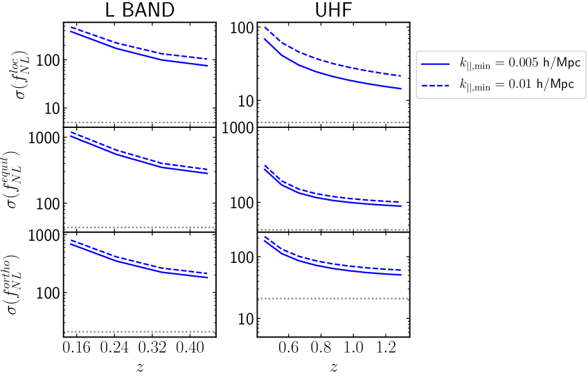
Figure 2: Cumulative forecast error from the combined HI IM power spectrum and bispectrum signal on $f_{\mathrm{NL}}^{\mathrm{loc}},f_{\mathrm{NL}}^{\mathrm{equil}},f_{\mathrm{NL}}^{\mathrm{orth}}$, for MeerKAT (L and UHF bands) in SD mode. Errors are shown for the two $k_{\parallel,{\rm min}}$ cuts in Eq. (34). Grey dotted line denotes the Planck error [8].

The Fisher matrix forecast results from the combined HI power spectrum and bispectrum signal are presented in this section. The cumulative $1\sigma$ forecast error for the amplitude of the three PNG shapes, in the case of the SKA precursor MeerKAT, is presented as a function of redshift in Fig. 2. The results for the two available MeerKAT bands are shown. The volumes probed by MeerKAT, as well as the scale limitations of the SD mode (see Sec. 7), restrict significantly the access to the large scales and therefore render the power spectrum contribution to the combined PNG signal minimal.

The UHF band corresponds to higher values of redshift, as well as to a more extended range, compared to the L-band, which leads to tighter constraints for all PNG cases. More precisely, almost an order of magnitude difference is observed between the forecasts originating from the two bands. The reason is that at higher redshifts, the observed physical volumes are larger and the accessible scales are probed with better resolution (i. ​e., smaller fundamental frequency). In addition, the clustering becomes more linear, so that the perturbative regime, where the tree-level description is adequate, can be pushed towards larger k-mode values (i. ​e., increasing $k_{\rm max}$ with redshift). These two effects provide an increasing number of triangles for the HI bispectrum, hence boosting significantly the PNG signal towards increasing redshift values and improving the forecasts.

These conditions are responsible for the decreasing trend towards higher redshift values, up to a saturation point, where increasing redshifts do not contribute significantly to the cumulative signal. This is because the additional triangle configurations provided by the ever-increasing perturbative regime are excluded by the limitations of the MeerKAT in SD mode (see Sec. 7). In particular, for redshifts $z\gtrsim 0.4$ and $z\gtrsim 1.1$, in the case of the L and UHF band respectively, only a small contribution to the non-Gaussian signal is observed, for all three PNG types.

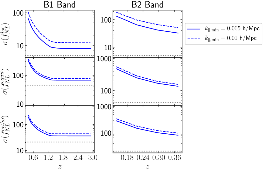
Figure 3: As in Fig. 2, for SKA1-MID in SD mode.

If a larger number of large-scale modes is lost to foreground contamination, i.e. $k_{\parallel,{\rm min}}=0.01\;\text{$h$/Mpc}$ (blue line), then all three PNG types are affected, with local PNG being the most affected. A harder $k_{\parallel,{\rm min}}$ cut-off decreases the available signal inside the volume of a survey. Due to the instrumental and survey specifications, the UHF band is more affected, since a significant amount of large-scale modes, and hence squeezed configurations, get removed with the $k_{\parallel,{\rm min}}$ cut. This affects local PNG the most, since on the one hand the local PNG bispectrum peaks on the squeezed triangles and on the other the consequent limited access to the large scales, reduces significantly the PNG signal of the scale-dependent bias correction in the HI power spectrum contribution. Equilateral PNG is affected the least, since the number of equilateral configurations, for which this template peaks, is not significantly reduced by the large-scale cut-offs. In fact, only a small number of the available equilateral triangles are excluded from each survey. Despite the fact that the power spectrum does not hold any constraining power on equilateral PNG (see Sec. 4), adding the power spectrum Fisher matrix to the bispectrum one, improves the PNG constraints over the latter. This is due to the enhanced signal provided by the power spectrum on the redshift-dependent free parameters, e.g. $b_{1}$.

Similar behaviour to the MeerKAT results can be seen in the case of the SKA1-MID experiment in SD mode (Fig. 3). An improvement towards higher redshift, due to the larger accessible volumes, can be also observed for both bands considered. Band B1 results reach a saturation point around $z\sim 1.3$, while saturation in B2 is only in the last redshift bins. Despite the large sky area and extended redshift range of B1 band, the cumulative results over the whole redshift range are only marginally better than those provided by the MeerKAT high-redshift band (see Table 3). The potential PNG signal in the power spectrum and bispectrum, provided by the high redshift slices ($z>1.4$) of SKA1-MID B1 band, is excluded by the fundamental limitations of the SD mode, i.e. the telescope beam, and therefore there is no significant information to be added in the forecasts (see left panels of Fig. 3). Note, that due to the accessible scale range of the B1 band, the power spectrum provides equivalent $f_{\rm NL}$ constraints to the bispectrum for local PNG, while for orthogonal PNG its contribution to the combined signal is marginal.

On the other hand, constraints in the low-redshift band B2 of SKA1-MID show a significant improvement ($\sim 2$ times) over those from MeerKAT L-band (see Figs. 2,3 and Table 3). This can be mainly attributed to the higher sky coverage, which offers a higher resolution in triangle-space, increasing the bispectrum signal, since both surveys span roughly the same redshift range. Also, the instrumental noise of SKA1-MID is only marginally better than that of MeerKAT. Analogously to the previous cases, the power spectrum PNG constraints are insignificant compared to those provided by the bispectrum. However, as before, the power spectrum improves indirectly the $f_{\rm NL}$ constraints, coming from the combined signal of the two correlators considered here, by reducing the correlation between the various redshift dependent parameters in $F_{\alpha\beta}^{P+B}$.

Considering the most optimistic results ($k_{\parallel,{\rm min}}=0.005\;\text{$h$/Mpc}$ cut-off) that originate from the cumulative signal over the total redshift range of SKA1-MID and MeerKAT (Table 3), we can see that the constraints are far from being competitive compared to the Planck measurements [151] (see also the grey dotted line in Figs. 2 and 3). Nonetheless, both MeerKAT UHF and SKA-MID B1 SD mode results are only few times worse than Planck, indicating that these HI IM data-sets can provide insightful preliminary tests on PNG and inflation.

The corresponding results in IF mode, for both surveys, are not shown. The specifications of MeerKAT and SKA-MID (see Tables 2 and 1) were not planned to function as a dedicated HI intensity mapping experiment. Therefore, they are not able to probe the corresponding scales that would make a bispectrum analysis viable in IF mode. In other words, IF mode excludes all the information available in these surveys.

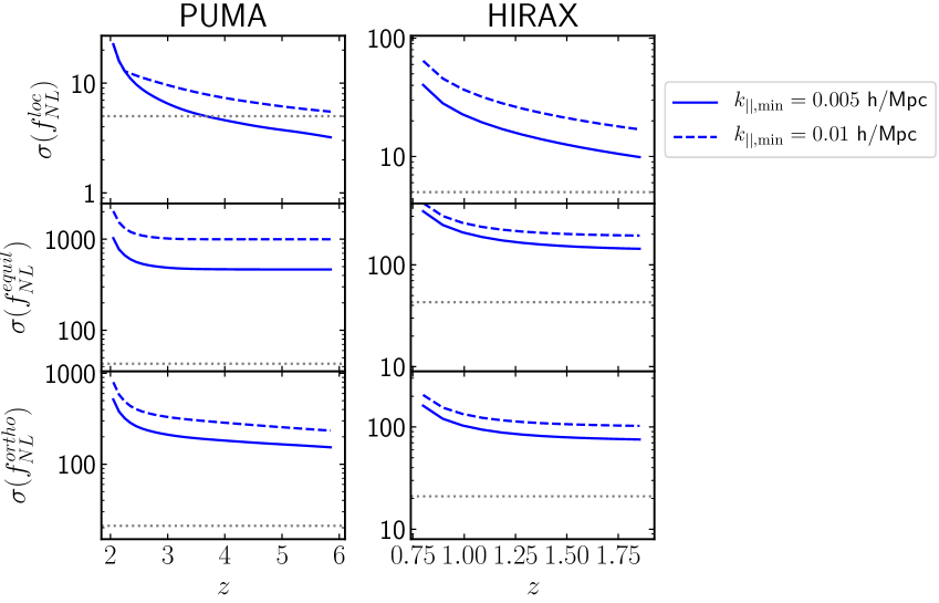
Figure 4: As in Fig. 2, for PUMA and HIRAX in SD mode.

A bispectrum analysis is favoured by surveys that function as interferometers, especially for packed arrays which beat the instrumental noise, since they can probe large to intermediate scales, forming a significant number of triangles, that enhances the HI bispectrum signal [64]. This is particularly important for PNG constraints coming from IM experiments. Conversely, a power spectrum analysis is more suitable for IM surveys that were designed to function in SD mode. They offer a sufficient range and resolution over linear scales, for the scale-dependent bias correction (see Eqs. (16) and (18)) to provide compelling constraints on PNG. This is particularly true for the local type, which has been shown to be sufficiently constrained by the SKA in SD mode [23, 25, 26, 27]. Nonetheless, due to the foregrounds and scale range probed by an experiment in SD mode, the bispectrum provides significantly tighter PNG constraints than the power spectrum for all the surveys discussed before, apart from SKA-MID B2 in the local PNG case. The latter is due to the fact that B2 offers a sufficient access to the large-scales, as well as the intermediate ones, providing an adequate amount of k-bins for the scale-dependent bias correction in the power spectrum to produce equivalent local PNG constraints to the bispectrum.

The argument can be further supported by the results shown in the case of PUMA and HIRAX. Both are designed for IF mode. Nevertheless, they can still function as SD experiments (see Table 1), where they can probe larger cosmological scales. The cumulative results from the the combined HI power spectrum and bispectrum signal are shown in Fig. 4. An immediate observation is that the signal of PUMA saturates after the first couple of redshift slices ($z\sim 2.7$), for equilateral and orthogonal PNG. The same holds for HIRAX, where the saturation is evident beyond $z\sim 1.4$. For both surveys, the SD beam excludes a significant number of modes that are well inside the perturbative regime, which otherwise would have been accessible to the surveys at the higher redshifts. This is a common trait of all the surveys considered here that function in SD mode, i. ​e., the bispectrum PNG signal is minimal beyond $z\gtrsim 1.4$, except for the full PUMA, which due to its large sky area coverage and redshift range, and its low instrumental noise, can provide sufficient PNG signal even at higher redshift values.

This explains the functional behaviour over redshift for the cumulative error in the equilateral and orthogonal PNG cases, coming from the combined power spectrum and bispectrum signal, since the constraints on $f_{\rm NL}$ originate mainly from the latter, while the contribution of the former remains minimal. On the other hand, for local PNG, the large volume of PUMA and HIRAX in SD mode provide adequate access to the large-scale regime, which leads to the power spectrum constraints being the tightest, since the SD-mode scale limitations restrict the squeezed configurations. The ever increasing linear regime, in conjunction with the increasing scale resolution (i.e. smaller $k_{f}$), results in improved local PNG power spectrum constraints towards high redshifts, justifying the observed redshift dependence of the error on $f_{\mathrm{NL}}^{\mathrm{loc}}$ seen in the top panels of Fig. 4.

Even with these improved specifications at hand, PUMA, as well as HIRAX, in SD mode do not offer competitive forecasts on equilateral and orthogonal PNG types compared to Planck (Table 3). In the case of local PNG, both surveys have the potential of providing competitive, or even improved in the case of PUMA, constraints relative to Planck. In addition, comparing the cumulative errors on equilateral and orthogonal PNG from both surveys with those provided by MeerKAT UHF and SKA1-MID B1, we observe that they are significantly less tight, e.g. PUMA SD-mode errors are $\sim 4$ times larger. This is because PUMA and HIRAX in SD mode do not utilise the notable bispectrum signal that lies in the higher redshift bins. On the other hand, for local PNG, PUMA is more promising, while HIRAX performs similarly to MeerKAT and SKA1-MID.

The PUMA and HIRAX results complement the study of [28], where both are considered in IF mode to forecast their power in constraining the three PNG types. A variety of observational effects, as well as different survey specifications, are studied in [28] to test their effect on the PNG signal, for both HI power spectrum and bispectrum. Comparing the results shown in Table 3 (SD mode results) with those presented in Table 2 of [28] (IF mode results), after considering the same $k_{\parallel,{\rm min}}$ sharp k-cuts (i.e. $k_{\parallel,{\rm min}}=0.01\;\text{$h$/Mpc}$ for the foregrounds) as well as using $N_{w}=1$ for the foreground wedge in IF mode, we see that HIRAX in SD mode provides almost $\sim 3-4$ times larger errors than in IF mode for the equilateral and orthogonal PNG cases, while for local the difference is reduced to $\sim 2$ times. In neither of the two possible set-ups (i.e. SD and IF modes) can HIRAX compete with the errors measured by Planck, although in IF mode they are only $\sim 2$ worse, as presented in [28].

In the case of PUMA, the change from SD to IF mode produces a significant difference in the PNG HI bispectrum forecasts. The SD constraints are far from being competitive, with the exception of local PNG, especially compared to smaller IM surveys, while for IF the PNG forecast errors can improve over those presented in Planck by a significant amount (see [28] for an extensive discussion). The large area covered by PUMA, leading to immense high-redshift volumes, offers a very high resolution in triangle space in the perturbative regime. This is utilised in the case of IF mode, in contrast to SD, to provide very competitive constraints on PNG from the HI bispectrum. Furthermore, the tightly packed array of PUMA reduces significantly the instrumental noise, making available to the analysis a wide range of scales. On the other hand, the power spectrum takes advantage of the large-scale regime probed by PUMA in SD mode and the combined power spectrum and bispectrum signal provides competitive constraints, even with a minimal bispectrum contribution. The comparison between SD and IF modes, in the cases of PUMA and HIRAX, further indicates that a HI bispectrum analysis, especially for PNG, is more suited to an IF than a SD experiment.

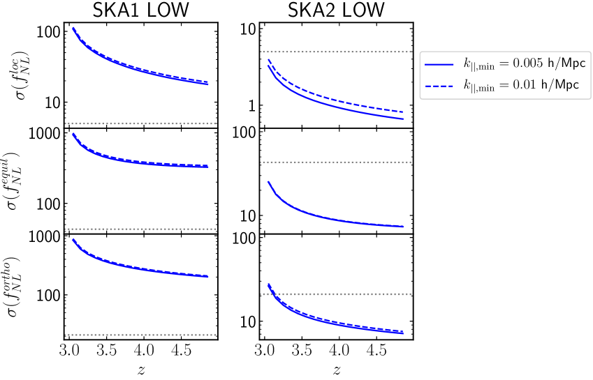
Figure 5: As in Fig. 2, for SKA1-LOW and SKA2-LOW in IF mode.

To further support this claim, we study PNG from the combined HI power spectrum and bispectrum signal for SKA1-LOW and its improved futuristic version SKA2-LOW (Table 2) in IF mode. The cumulative errors on PNG are presented in Fig. 5 as a function of redshift, while the errors from the cumulative signal over the whole redshift range are presented in Table 3 for all three PNG cases. The SKA1-LOW experiment was designed as an interferometer in order to study the epoch of reionisation. Nonetheless, the high redshifts provided, where the Universe is more linear, makes it ideal for a combined power spectrum and bispectrum PNG analysis.

The cumulative results show a constant improvement over the whole redshift range, indicating that the scales from the growing perturbative regime, which are important for the HI bispectrum signal, are accessed in IF mode, especially those in the high redshift slices. Furthermore, the large scales probed by SKA-LOW provide enough PNG signal in order for the power spectrum to be the main contributor in the combined signal. However, the low number of dishes, as well as the small sky area probed, increase the instrumental noise, thereby killing a significant amount of the available signal. These effects lead to non-competitive forecasts, in most cases even less than the low-redshift counterparts of MeerKAT and SKA1-MID.

Nevertheless, the improved version, SKA2-LOW, has the experimental settings, and in particular the large number of dishes, needed to deliver unprecedented constraints on PNG of all three types considered here, $\sigma(f_{\mathrm{NL}}^{\mathrm{loc}})\sim 0.7$, $\sigma(f_{\mathrm{NL}}^{\mathrm{equil}})\sim 13$ and $\sigma(f_{\mathrm{NL}}^{\mathrm{orth}})\sim 8$. The bispectrum provides again here the bulk of the combined PNG signal, while the power spectrum in the case of local PNG, due to the extremely large volumes probed, offers a competitive amount of information with respect to the bispectrum, especially in the very high redshift slices. In particular, SKA2-LOW improves over the Planck measurements already by utilising the bispectrum signal of the first couple of redshift slices (right panel of Fig. 5), in the case of the optimistic $k_{\parallel,{\rm min}}$ cuts. This is even true for the pessimistic sharp cut-off in the case of the equilateral PNG. This type of PNG is usually the least constrained by LSS surveys. Hence, the forecasts from SKA2-LOW on equilateral PNG indicate the great prospect that may lie within future IM interferometer surveys. The cumulative error shows a continuous decrease as a function of redshift, where it saturates only at the last high redshift bins. Excluding more large scales due to the foregrounds, still produces very competitive constraints (Table 3), where local and orthogonal are affected the most due to the functional form of their templates (see Sec. 2).

9 Discussion

The goal of this paper was to study the combined HI IM power spectrum and bispectrum of current and planned experiments, in configurations not yet considered, in order to find the ideal set-up for such an analysis, in particular one targeting PNG. In the case of the MeerKAT, SKA-MID, HIRAX and PUMA experiments, we considered SD mode, while for SKA1-LOW and SKA2-LOW we considered IF mode. To determine the HI IM power spectrum and bispectrum we reviewed the matter model, the HI bias model, and the inclusion of RSD and PNG in the two correlators. This work is also intended to complement other power spectrum and bispectrum studies with LSS, using HI IM (see e.g. [152, 153, 154, 28, 155, 156, 157, 158]) and optical and radio continuum galaxy surveys (see e.g. [62]).

	MEERKAT (SD)		SKA-MID (SD)		PUMA (SD)	HIRAX (SD)	SKA1-LOW (IF)	SKA2-LOW (IF)
PNG Cases	L-BAND	UHF	BAND 1	BAND 2
Local	77 (105)	15 (22)	8 (12)	33 (52)	3 (6)	10 (17)	18 (19)	0.7 (0.8)
Equilateral	494 (578)	141 (166)	52 (60)	232 (273)	553 (1325)	189 (274)	607 (653)	12.5 (12.8)
Orthogonal	234 (288)	63 (80)	47 (60)	105 (134)	154 (236)	95 (139)	215 (221)	7.6 (8)

Table 3: Bispectrum forecasts for 1$\sigma$ marginalised errors on $f_{\mathrm{NL}}^{\mathrm{loc}},f_{\mathrm{NL}}^{\mathrm{equil}},f_{\mathrm{NL}}^{\mathrm{orth}}$, from the cumulative signal over the total redshift range. A foreground-imposed cut $k_{\parallel,{\rm min}}=0.005\;\text{$h$/Mpc}$ is used. Errors in parenthesis correspond to a less optimistic $k_{\parallel,{\rm min}}=0.01\;\text{$h$/Mpc}$.

We started by analysing the prospects of the SKA precursor MeerKAT, as it is already operational. In Fig. 2 we showed the forecasted cumulative errors for the three $f_{\rm NL}$ parameters as a function of redshift for the two MeerKAT available bands. An immediate observation is that the UHF band performs much better than the L-band. This comes as no surprise, because towards higher redshifts the observed physical volume increases, hence more triangles, as well as large-scale modes, from which to extract information. By the same token all curves in Fig. 2 decrease with the increase of redshift, up to signal saturation. Also, as expected, including information from larger scales, i.e., having a lower $k_{\rm min}$ (red line), improves the forecasted errors. Although the MeerKAT is very far from providing a competitive error bar on the combined HI IM power spectrum and bispectrum signal (especially in comparison with the latest Planck results [8], shown as the grey dashed line) it will provide an insightful data-set for preliminary tests. The cumulative constraints from all redshift bins, in the case of the pessimistic foreground cuts, are only few times worse than Planck (see Table 3).

SKA1-MID provided improved results relative to MeerKAT (see Fig. 3). Such improvements mainly come from the larger sky area covered by the surveys, as the instrumental noise of SKA1-MID is only marginally better than MeerKAT’s. Both SKA1-MID bands follow the same trends as the MeerKAT ones, i.e., higher redshift bins contain a larger volume, providing more available triangles and $k$-bins located in the large-scale regime from which to extract information. Despite the improvement per redshift bin, the cumulative result (see Table 3) from the high-redshift SKA-MID survey is only marginally better than that from the MeerKAT survey. On the other hand, for the low-redshift bands, the increased volume has a considerable impact on the forecasted error (by a factor $\sim 2$).

Both MeerKAT and SKA-MID were not planned as dedicated HI intensity mapping facilities. Nevertheless, they can be effective for the HI IM power spectrum. On the other hand, both HIRAX and PUMA were designed as dedicated experiments to extract the HI power spectrum in IF mode. Despite being designed as dish interferometers, they can still work as SD-mode experiments and therefore probe large cosmological scales: results are shown in Fig. 4. These constraints are far behind the IF mode constraints presented in [28].

Finally, we studied the combined HI IM power spectrum and bispectrum with SKA-LOW, which is designed as an interferometer to do HI IM of the epoch of reionisation. Nevertheless, its frequency range covers redshifts down to $z=3$ and so it can be used in IF mode for post-reionisation constraints on PNG. Our results are shown in Fig. 5, and we concluded that while SKA1-LOW will provide results similar to its low-redshift MID counterpart, SKA2-LOW will have enough information to hit the Planck level in single redshift bins, with cumulative constraints at unprecedented levels. Despite attaining $\sigma(f_{\mathrm{NL}}^{\mathrm{loc}})\sim 1$, SKA2-LOW is very futuristic.

In Table 3 we summarised the results from all the experimental settings considered in this paper. While the local shape is the easiest to measure in all experiments, the equilateral shape is always harder. In the case of the bispectrum, an explanation is due to the number of triangles available in a finite volume as well as the strength (or weakness) of the signal. The number of equilateral triangles inside a fixed scale range is the same as the number of individual k-bins, while there are more squeezed configurations that can be formed inside the same range. The number of the latter increases significantly if enough large scales are accessible to the survey. Furthermore, the equilateral PNG template peaks on the same configurations as the gravitational part of the bispectrum (equilateral triangles). The latter has a few orders of magnitude larger amplitude, making the disentanglement of the two a tedious process. Note, that for equilateral PNG, the power spectrum has no constraining power on $f_{\mathrm{NL}}^{\mathrm{equil}}$ (see section 4), making the bispectrum the sole contributor to the PNG signal. Therefore, equilateral PNG is the least constrained shape from LSS surveys (see [62] for a discussion). More importantly, despite the ever-larger volumes of the surveys, the cuts on $k_{\parallel}$ from foregrounds in the signal impose limitations on what one can do with the observed signal. We imposed two cuts at $k_{\parallel,{\rm min}}=0.005\;\text{$h$/Mpc}$ and a less optimistic $k_{\parallel,{\rm min}}=0.01\;\text{$h$/Mpc}$. Fundamentally we know that for SD mode, the inclusion of larger scales improves the measurements substantially, especially for local PNG in the case of the power spectrum. This is also true in the case of the HI bispectrum, as it is shown in Table 3. Hence it is crucial to obtain the signal from the larger scales instead of discarding it altogether.

One can try to disentangle the HI signal from the foreground signal using clever statistical methods. Indeed, a substantial amount of work has been done at the HI power spectrum level with blind foreground subtraction methods (see e.g. [120] for an extensive study of different foreground subtraction methods and [159, 160] for more recent studies). In general, blind foreground methods perform very well on small scales but do not recover well the large scales which are needed to improve bispectrum measurements. In practice, one would need to fit transfer functions based on simulations to fully reconstruct them. Alternatively one can look to reconstruct the large scales from other available scales using quadratic estimators. This has been proposed recently in [161] and further explored in [162] were RSD and bias models where included in their original work. This opens a new window to reconstruct large scales in HI intensity mapping that we will pursue in the future.

Our results indicate that a HI bispectrum analysis, and in particular a PNG-oriented one, is better done using an IF experiment with a packed array, i.e. high-density dish distribution. Although more and more dishes help to improve the noise, the two configurations considered provide information in disjoint scale ranges. While the size of the dish imposes a minimum accessible scale in SD modes, in IF mode it becomes the largest accessible scale. Hence, for bispectrum studies, one should choose a survey that includes the scales containing the bulk of the information, which are smaller but still linear scales. These are better probed by IF mode. In addition, IF surveys can be further improved by a large sky coverage and high redshift reach. For the power spectrum, the bulk of the PNG signal, especially for the local case, originates from the large-scale regime, due to the scale-dependent bias correction. This makes SD-mode experiments ideal for a power spectrum analysis. Nonetheless, we show that in the case of small-volume surveys in SD mode, the bispectrum can still outperform power spectrum constraints. In the case where the large-scale regime is probed with sufficient resolution, the power spectrum provides the tightest constraints, in particular for the local PNG. In this case, for surveys that additionally offer access to scales towards the end of the linear regime, the power spectrum and bispectrum provide equivalent constraints and a combined analysis would optimally utilise the available PNG signal. Proposed surveys that fit these criteria, like SKA2-LOW and PUMA (Full) (see [28]), make ideal candidates for putting tight constraints on the amplitude of PNG, including the elusive equilateral type, and shedding light on the inflationary epoch of the primordial Universe.

References

- Planck Collaboration et al. [2020a] Planck Collaboration, N. Aghanim, Y. Akrami, M. Ashdown, J. Aumont, C. Baccigalupi, M. Ballardini, A. J. Banday, R. B. Barreiro, N. Bartolo, S. Basak, R. Battye, K. Benabed, J. P. Bernard, M. Bersanelli, P. Bielewicz, J. J. Bock, J. R. Bond, J. Borrill, F. R. Bouchet, F. Boulanger, M. Bucher, C. Burigana, R. C. Butler, E. Calabrese, J. F. Cardoso, J. Carron, A. Challinor, H. C. Chiang, J. Chluba, L. P. L. Colombo, C. Combet, D. Contreras, B. P. Crill, F. Cuttaia, P. de Bernardis, G. de Zotti, J. Delabrouille, J. M. Delouis, E. Di Valentino, J. M. Diego, O. Doré, M. Douspis, A. Ducout, X. Dupac, S. Dusini, G. Efstathiou, F. Elsner, T. A. Enßlin, H. K. Eriksen, Y. Fantaye, M. Farhang, J. Fergusson, R. Fernandez-Cobos, F. Finelli, F. Forastieri, M. Frailis, A. A. Fraisse, E. Franceschi, A. Frolov, S. Galeotta, S. Galli, K. Ganga, R. T. Génova-Santos, M. Gerbino, T. Ghosh, J. González-Nuevo, K. M. Górski, S. Gratton, A. Gruppuso, J. E. Gudmundsson, J. Hamann, W. Handley, F. K. Hansen, D. Herranz, S. R. Hildebrandt, E. Hivon, Z. Huang, A. H. Jaffe, W. C. Jones, A. Karakci, E. Keihänen, R. Keskitalo, K. Kiiveri, J. Kim, T. S. Kisner, L. Knox, N. Krachmalnicoff, M. Kunz, H. Kurki-Suonio, G. Lagache, J. M. Lamarre, A. Lasenby, M. Lattanzi, C. R. Lawrence, M. Le Jeune, P. Lemos, J. Lesgourgues, F. Levrier, A. Lewis, M. Liguori, P. B. Lilje, M. Lilley, V. Lindholm, M. López-Caniego, P. M. Lubin, Y. Z. Ma, J. F. Macías-Pérez, G. Maggio, D. Maino, N. Mandolesi, A. Mangilli, A. Marcos-Caballero, M. Maris, P. G. Martin, M. Martinelli, E. Martínez-González, S. Matarrese, N. Mauri, J. D. McEwen, P. R. Meinhold, A. Melchiorri, A. Mennella, M. Migliaccio, M. Millea, S. Mitra, M. A. Miville-Deschênes, D. Molinari, L. Montier, G. Morgante, A. Moss, P. Natoli, H. U. Nørgaard-Nielsen, L. Pagano, D. Paoletti, B. Partridge, G. Patanchon, H. V. Peiris, F. Perrotta, V. Pettorino, F. Piacentini, L. Polastri, G. Polenta, J. L. Puget, J. P. Rachen, M. Reinecke, M. Remazeilles, A. Renzi, G. Rocha, C. Rosset, G. Roudier, J. A. Rubiño-Martín, B. Ruiz-Granados, L. Salvati, M. Sandri, M. Savelainen, D. Scott, E. P. S. Shellard, C. Sirignano, G. Sirri, L. D. Spencer, R. Sunyaev, A. S. Suur-Uski, J. A. Tauber, D. Tavagnacco, M. Tenti, L. Toffolatti, M. Tomasi, T. Trombetti, L. Valenziano, J. Valiviita, B. Van Tent, L. Vibert, P. Vielva, F. Villa, N. Vittorio, B. D. Wand elt, I. K. Wehus, M. White, S. D. M. White, A. Zacchei, A. Zonca, Planck 2018 results. VI. Cosmological parameters, A&A 641 (2020a) A6. doi:10.1051/0004-6361/201833910. arXiv:1807.06209.
- Planck Collaboration et al. [2020b] Planck Collaboration, N. Aghanim, Y. Akrami, F. Arroja, M. Ashdown, J. Aumont, C. Baccigalupi, M. Ballardini, A. J. Banday, R. B. Barreiro, N. Bartolo, S. Basak, R. Battye, K. Benabed, J. P. Bernard, M. Bersanelli, P. Bielewicz, J. J. Bock, J. R. Bond, J. Borrill, F. R. Bouchet, F. Boulanger, M. Bucher, C. Burigana, R. C. Butler, E. Calabrese, J. F. Cardoso, J. Carron, B. Casaponsa, A. Challinor, H. C. Chiang, L. P. L. Colombo, C. Combet, D. Contreras, B. P. Crill, F. Cuttaia, P. de Bernardis, G. de Zotti, J. Delabrouille, J. M. Delouis, F. X. Désert, E. Di Valentino, C. Dickinson, J. M. Diego, S. Donzelli, O. Doré, M. Douspis, A. Ducout, X. Dupac, G. Efstathiou, F. Elsner, T. A. Enßlin, H. K. Eriksen, E. Falgarone, Y. Fantaye, J. Fergusson, R. Fernandez-Cobos, F. Finelli, F. Forastieri, M. Frailis, E. Franceschi, A. Frolov, S. Galeotta, S. Galli, K. Ganga, R. T. Génova-Santos, M. Gerbino, T. Ghosh, J. González-Nuevo, K. M. Górski, S. Gratton, A. Gruppuso, J. E. Gudmundsson, J. Hamann, W. Hand ley, F. K. Hansen, G. Helou, D. Herranz, S. R. Hildebrandt, E. Hivon, Z. Huang, A. H. Jaffe, W. C. Jones, A. Karakci, E. Keihänen, R. Keskitalo, K. Kiiveri, J. Kim, T. S. Kisner, L. Knox, N. Krachmalnicoff, M. Kunz, H. Kurki-Suonio, G. Lagache, J. M. Lamarre, M. Langer, A. Lasenby, M. Lattanzi, C. R. Lawrence, M. Le Jeune, J. P. Leahy, J. Lesgourgues, F. Levrier, A. Lewis, M. Liguori, P. B. Lilje, M. Lilley, V. Lindholm, M. López-Caniego, P. M. Lubin, Y. Z. Ma, J. F. Macías-Pérez, G. Maggio, D. Maino, N. Mand olesi, A. Mangilli, A. Marcos-Caballero, M. Maris, P. G. Martin, M. Martinelli, E. Martínez-González, S. Matarrese, N. Mauri, J. D. McEwen, P. D. Meerburg, P. R. Meinhold, A. Melchiorri, A. Mennella, M. Migliaccio, M. Millea, S. Mitra, M. A. Miville-Deschênes, D. Molinari, A. Moneti, L. Montier, G. Morgante, A. Moss, S. Mottet, M. Münchmeyer, P. Natoli, H. U. Nørgaard-Nielsen, C. A. Oxborrow, L. Pagano, D. Paoletti, B. Partridge, G. Patanchon, T. J. Pearson, M. Peel, H. V. Peiris, F. Perrotta, V. Pettorino, F. Piacentini, L. Polastri, G. Polenta, J. L. Puget, J. P. Rachen, M. Reinecke, M. Remazeilles, C. Renault, A. Renzi, G. Rocha, C. Rosset, G. Roudier, J. A. Rubiño-Martín, B. Ruiz-Granados, L. Salvati, M. Sandri, M. Savelainen, D. Scott, E. P. S. Shellard, M. Shiraishi, C. Sirignano, G. Sirri, L. D. Spencer, R. Sunyaev, A. S. Suur-Uski, J. A. Tauber, D. Tavagnacco, M. Tenti, L. Terenzi, L. Toffolatti, M. Tomasi, T. Trombetti, J. Valiviita, B. Van Tent, L. Vibert, P. Vielva, F. Villa, N. Vittorio, B. D. Wand elt, I. K. Wehus, M. White, S. D. M. White, A. Zacchei, A. Zonca, Planck 2018 results. I. Overview and the cosmological legacy of Planck, A&A 641 (2020b) A1. doi:10.1051/0004-6361/201833880. arXiv:1807.06205.
- de Mattia et al. [2020] A. de Mattia, V. Ruhlmann-Kleider, A. Raichoor, A. J. Ross, A. Tamone, C. Zhao, S. Alam, S. Avila, E. Burtin, J. Bautista, F. Beutler, J. Brinkmann, J. R. Brownstein, M. J. Chapman, C.-H. Chuang, J. Comparat, H. du Mas des Bourboux, K. S. Dawson, A. de la Macorra, H. Gil-Marín, V. Gonzalez-Perez, C. Gorgoni, J. Hou, H. Kong, S. Lin, S. Nadathur, J. A. Newman, E.-M. Mueller, W. J. Percival, M. Rezaie, G. Rossi, D. P. Schneider, P. Tiwari, M. Vivek, Y. Wang, G.-B. Zhao, The Completed SDSS-IV extended Baryon Oscillation Spectroscopic Survey: measurement of the BAO and growth rate of structure of the emission line galaxy sample from the anisotropic power spectrum between redshift 0.6 and 1.1, arXiv e-prints (2020) arXiv:2007.09008. arXiv:2007.09008.
- Raichoor et al. [2020] A. Raichoor, A. de Mattia, A. J. Ross, C. Zhao, S. Alam, S. Avila, J. Bautista, J. Brinkmann, J. R. Brownstein, E. Burtin, M. J. Chapman, C.-H. Chuang, J. Comparat, K. S. Dawson, A. Dey, H. du Mas des Bourboux, J. Elvin-Poole, V. Gonzalez-Perez, C. Gorgoni, J.-P. Kneib, H. Kong, D. Lang, J. Moustakas, A. D. Myers, E.-M. Müller, S. Nadathur, J. A. Newman, W. J. Percival, M. Rezaie, G. Rossi, V. Ruhlmann-Kleider, D. J. Schlegel, D. P. Schneider, H.-J. Seo, A. Tamone, J. L. Tinker, R. Tojeiro, M. Vivek, C. Yèche, G.-B. Zhao, The completed SDSS-IV extended Baryon Oscillation Spectroscopic Survey: Large-scale Structure Catalogues and Measurement of the isotropic BAO between redshift 0.6 and 1.1 for the Emission Line Galaxy Sample, arXiv e-prints (2020) arXiv:2007.09007. arXiv:2007.09007.
- Abbott et al. [2019] T. M. C. Abbott, A. Alarcon, S. Allam, P. Andersen, F. Andrade-Oliveira, J. Annis, J. Asorey, S. Avila, D. Bacon, N. Banik, B. A. Bassett, E. Baxter, K. Bechtol, M. R. Becker, G. M. Bernstein, E. Bertin, J. Blazek, S. L. Bridle, D. Brooks, D. Brout, D. L. Burke, J. Calcino, H. Camacho, A. Campos, A. Carnero Rosell, D. Carollo, M. Carrasco Kind, J. Carretero, F. J. Castander, R. Cawthon, P. Challis, K. C. Chan, C. Chang, M. Childress, M. Crocce, C. E. Cunha, C. B. D’Andrea, L. N. da Costa, C. Davis, T. M. Davis, J. De Vicente, D. L. DePoy, J. DeRose, S. Desai, H. T. Diehl, J. P. Dietrich, S. Dodelson, P. Doel, A. Drlica-Wagner, T. F. Eifler, J. Elvin-Poole, J. Estrada, A. E. Evrard, E. Fernandez, B. Flaugher, R. J. Foley, P. Fosalba, J. Frieman, L. Galbany, J. García-Bellido, M. Gatti, E. Gaztanaga, D. W. Gerdes, T. Giannantonio, K. Glazebrook, D. A. Goldstein, D. Gruen, R. A. Gruendl, J. Gschwend, G. Gutierrez, W. G. Hartley, S. R. Hinton, D. L. Hollowood, K. Honscheid, J. K. Hoormann, B. Hoyle, D. Huterer, B. Jain, D. J. James, M. Jarvis, T. Jeltema, E. Kasai, S. Kent, R. Kessler, A. G. Kim, N. Kokron, E. Krause, R. Kron, K. Kuehn, N. Kuropatkin, O. Lahav, J. Lasker, P. Lemos, G. F. Lewis, T. S. Li, C. Lidman, M. Lima, H. Lin, E. Macaulay, N. MacCrann, M. A. G. Maia, M. March, J. Marriner, J. L. Marshall, P. Martini, R. G. McMahon, P. Melchior, F. Menanteau, R. Miquel, J. J. Mohr, E. Morganson, J. Muir, A. Möller, E. Neilsen, R. C. Nichol, B. Nord, R. L. C. Ogando, A. Palmese, Y. C. Pan, H. V. Peiris, W. J. Percival, A. A. Plazas, A. Porredon, J. Prat, A. K. Romer, A. Roodman, R. Rosenfeld, A. J. Ross, E. S. Rykoff, S. Samuroff, C. Sánchez, E. Sanchez, V. Scarpine, R. Schindler, M. Schubnell, D. Scolnic, L. F. Secco, S. Serrano, I. Sevilla-Noarbe, R. Sharp, E. Sheldon, M. Smith, M. Soares-Santos, F. Sobreira, N. E. Sommer, E. Swann, M. E. C. Swanson, G. Tarle, D. Thomas, R. C. Thomas, M. A. Troxel, B. E. Tucker, S. A. Uddin, P. Vielzeuf, A. R. Walker, M. Wang, N. Weaverdyck, R. H. Wechsler, J. Weller, B. Yanny, B. Zhang, Y. Zhang, J. Zuntz, DES Collaboration, Cosmological Constraints from Multiple Probes in the Dark Energy Survey, Phys. Rev. Lett. 122 (2019) 171301. doi:10.1103/PhysRevLett.122.171301. arXiv:1811.02375.
- Joachimi et al. [2020] B. Joachimi, C. A. Lin, M. Asgari, T. Tröster, C. Heymans, H. Hildebrandt, F. Köhlinger, A. G. Sánchez, A. H. Wright, M. Bilicki, C. Blake, J. L. van den Busch, M. Crocce, A. Dvornik, T. Erben, F. Getman, B. Giblin, H. Hoekstra, A. Kannawadi, K. Kuijken, N. R. Napolitano, P. Schneider, R. Scoccimarro, E. Sellentin, H. Y. Shan, M. von Wietersheim-Kramsta, J. Zuntz, KiDS-1000 Methodology: Modelling and inference for joint weak gravitational lensing and spectroscopic galaxy clustering analysis, arXiv e-prints (2020) arXiv:2007.01844. arXiv:2007.01844.
- Abbott et al. [2019] T. M. C. Abbott, F. B. Abdalla, A. Alarcon, S. Allam, J. Annis, S. Avila, K. Aylor, M. Banerji, N. Banik, E. J. Baxter, K. Bechtol, M. R. Becker, B. A. Benson, G. M. Bernstein, E. Bertin, F. Bianchini, J. Blazek, L. E. Bleem, S. L. Bridle, D. Brooks, E. Buckley-Geer, D. L. Burke, J. E. Carlstrom, A. Carnero Rosell, M. Carrasco Kind, J. Carretero, F. J. Castander, R. Cawthon, C. Chang, C. L. Chang, H. M. Cho, A. Choi, R. Chown, T. M. Crawford, A. T. Crites, M. Crocce, C. E. Cunha, C. B. D’Andrea, L. N. da Costa, C. Davis, T. de Haan, J. DeRose, S. Desai, J. De Vicente, H. T. Diehl, J. P. Dietrich, M. A. Dobbs, S. Dodelson, P. Doel, A. Drlica-Wagner, T. F. Eifler, J. Elvin-Poole, W. B. Everett, B. Flaugher, P. Fosalba, O. Friedrich, J. Frieman, J. García-Bellido, M. Gatti, E. Gaztanaga, E. M. George, D. W. Gerdes, T. Giannantonio, D. Gruen, R. A. Gruendl, J. Gschwend, G. Gutierrez, N. W. Halverson, N. L. Harrington, W. G. Hartley, G. P. Holder, D. L. Hollowood, W. L. Holzapfel, K. Honscheid, Z. Hou, B. Hoyle, J. D. Hrubes, D. Huterer, B. Jain, D. J. James, M. Jarvis, T. Jeltema, M. W. G. Johnson, M. D. Johnson, S. Kent, D. Kirk, L. Knox, N. Kokron, E. Krause, K. Kuehn, O. Lahav, A. T. Lee, E. M. Leitch, T. S. Li, M. Lima, H. Lin, D. Luong-Van, N. MacCrann, M. A. G. Maia, A. Manzotti, D. P. Marrone, J. L. Marshall, P. Martini, J. J. McMahon, F. Menanteau, S. S. Meyer, R. Miquel, L. M. Mocanu, J. J. Mohr, J. Muir, T. Natoli, A. Nicola, B. Nord, Y. Omori, S. Padin, S. Pandey, A. A. Plazas, A. Porredon, J. Prat, C. Pryke, M. M. Rau, C. L. Reichardt, R. P. Rollins, A. K. Romer, A. Roodman, A. J. Ross, E. Rozo, J. E. Ruhl, E. S. Rykoff, S. Samuroff, C. Sánchez, E. Sanchez, J. T. Sayre, V. Scarpine, K. K. Schaffer, L. F. Secco, S. Serrano, I. Sevilla-Noarbe, E. Sheldon, E. Shirokoff, G. Simard, M. Smith, M. Soares-Santos, F. Sobreira, Z. Staniszewski, A. A. Stark, K. T. Story, E. Suchyta, M. E. C. Swanson, G. Tarle, D. Thomas, M. A. Troxel, D. L. Tucker, K. Vanderlinde, J. D. Vieira, P. Vielzeuf, V. Vikram, A. R. Walker, R. H. Wechsler, J. Weller, R. Williamson, W. L. K. Wu, B. Yanny, O. Zahn, Y. Zhang, J. Zuntz, DES, SPT Collaborations, Dark Energy Survey year 1 results: Joint analysis of galaxy clustering, galaxy lensing, and CMB lensing two-point functions, Phys. Rev. D 100 (2019) 023541. doi:10.1103/PhysRevD.100.023541. arXiv:1810.02322.
- Akrami et al. [2020] Y. Akrami, et al. (Planck), Planck 2018 results. IX. Constraints on primordial non-Gaussianity, Astron. Astrophys. 641 (2020) A9. doi:10.1051/0004-6361/201935891. arXiv:1905.05697.
- Sefusatti and Komatsu [2007] E. Sefusatti, E. Komatsu, The Bispectrum of Galaxies from High-Redshift Galaxy Surveys: Primordial Non-Gaussianity and Non-Linear Galaxy Bias, Phys. Rev. D 76 (2007) 083004. doi:10.1103/PhysRevD.76.083004. arXiv:0705.0343.
- Carbone et al. [2008] C. Carbone, L. Verde, S. Matarrese, Non-Gaussian Halo Bias and Future Galaxy Surveys, ApJ 684 (2008) L1. doi:10.1086/592020. arXiv:0806.1950.
- Giannantonio et al. [2014] T. Giannantonio, A. J. Ross, W. J. Percival, R. Crittenden, D. Bacher, M. Kilbinger, R. Nichol, J. Weller, Improved Primordial Non-Gaussianity Constraints from Measurements of Galaxy Clustering and the Integrated Sachs-Wolfe Effect, Phys. Rev. D 89 (2014) 023511. doi:10.1103/PhysRevD.89.023511. arXiv:1303.1349.
- Karagiannis et al. [2014] D. Karagiannis, T. Shanks, N. P. Ross, Search for primordial non-Gaussianity in the quasars of SDSS-III BOSS DR9, Mon. Not. Roy. Astron. Soc. 441 (2014) 486–502. doi:10.1093/mnras/stu590. arXiv:1310.6716.
- Castorina et al. [2019] E. Castorina, et al., Redshift-weighted constraints on primordial non-Gaussianity from the clustering of the eBOSS DR14 quasars in Fourier space, JCAP 09 (2019) 010. doi:10.1088/1475-7516/2019/09/010. arXiv:1904.08859.
- Blake and Wall [2002] C. Blake, J. Wall, Measurement of the angular correlation function of radio galaxies from the NRAO VLA Sky Survey, Mon. Not. Roy. Astron. Soc. 329 (2002) L37–L41. doi:10.1046/j.1365-8711.2002.05163.x. arXiv:astro-ph/0111328.
- Overzier et al. [2003] R. Overzier, H. Rottgering, R. Rengelink, R. Wilman, The spatial clustering of radio sources in NVSS and FIRST: implications for galaxy clustering evolution, Astron. Astrophys. 405 (2003) 53–72. doi:10.1051/0004-6361:20030527. arXiv:astro-ph/0304160.
- Martin et al. [2012] A. M. Martin, R. Giovanelli, M. P. Haynes, L. Guzzo, The Clustering Characteristics of HI-selected Galaxies from the 40% ALFALFA Survey, ApJ 750 (2012) 38. doi:10.1088/0004-637X/750/1/38. arXiv:1202.6005.
- Papastergis et al. [2013] E. Papastergis, R. Giovanelli, M. P. Haynes, A. Rodríguez-Puebla, M. G. Jones, The Clustering of ALFALFA Galaxies: Dependence on H Mass, Relationship with Optical Samples, and Clues of Host Halo Properties, Astrophys. J. 776 (2013) 43. doi:10.1088/0004-637X/776/1/43. arXiv:1308.2661.
- Bharadwaj et al. [2001] S. Bharadwaj, B. Nath, B. B. Nath, S. K. Sethi, Using HI to probe large scale structures at , J. Astrophys. Astron. 22 (2001) 21. doi:10.1007/BF02933588. arXiv:astro-ph/0003200.
- Battye et al. [2004] R. A. Battye, R. D. Davies, J. Weller, Neutral hydrogen surveys for high redshift galaxy clusters and proto-clusters, Mon. Not. Roy. Astron. Soc. 355 (2004) 1339–1347. doi:10.1111/j.1365-2966.2004.08416.x. arXiv:astro-ph/0401340.
- Wyithe and Loeb [2007] J. S. B. Wyithe, A. Loeb, Fluctuations in 21-cm emission after reionization, Monthly Notices of the Royal Astronomical Society 383 (2007) 606–614. URL: https://doi.org/10.1111/j.1365-2966.2007.12568.x. doi:10.1111/j.1365-2966.2007.12568.x. arXiv:https://academic.oup.com/mnras/article-pdf/383/2/606/18572114/mnras0383-0606.pdf.
- Chang et al. [2008] T.-C. Chang, U.-L. Pen, J. B. Peterson, P. McDonald, Baryon Acoustic Oscillation Intensity Mapping of Dark Energy, Phys. Rev. Lett. 100 (2008) 091303. doi:10.1103/PhysRevLett.100.091303. arXiv:0709.3672.
- Battye et al. [2013] R. A. Battye, I. W. A. Browne, C. Dickinson, G. Heron, B. Maffei, A. Pourtsidou, H I intensity mapping: a single dish approach, MNRAS 434 (2013) 1239–1256. doi:10.1093/mnras/stt1082. arXiv:1209.0343.
- Camera et al. [2013] S. Camera, M. G. Santos, P. G. Ferreira, L. Ferramacho, Cosmology on Ultralarge Scales with Intensity Mapping of the Neutral Hydrogen 21 cm Emission: Limits on Primordial Non-Gaussianity, Physical Review Letters 111 (2013) 171302. doi:10.1103/PhysRevLett.111.171302. arXiv:1305.6928.
- Xu et al. [2015] Y. Xu, X. Wang, X. Chen, Forecasts on the Dark Energy and Primordial Non-Gaussianity Observations with the Tianlai Cylinder Array, Astrophys. J. 798 (2015) 40. doi:10.1088/0004-637X/798/1/40. arXiv:1410.7794.
- Fonseca et al. [2015] J. Fonseca, S. Camera, M. Santos, R. Maartens, Hunting down horizon-scale effects with multi-wavelength surveys, Astrophys. J. Lett. 812 (2015) L22. doi:10.1088/2041-8205/812/2/L22. arXiv:1507.04605.
- Fonseca et al. [2017] J. Fonseca, R. Maartens, M. G. Santos, Probing the primordial Universe with MeerKAT and DES, MNRAS 466 (2017) 2780–2786. doi:10.1093/mnras/stw3248. arXiv:1611.01322.
- Ballardini et al. [2019] M. Ballardini, W. L. Matthewson, R. Maartens, Constraining primordial non-Gaussianity using two galaxy surveys and CMB lensing, Mon. Not. Roy. Astron. Soc. 489 (2019) 1950–1956. doi:10.1093/mnras/stz2258. arXiv:1906.04730.
- Karagiannis et al. [2020] D. Karagiannis, A. Slosar, M. Liguori, Forecasts on Primordial non-Gaussianity from 21 cm Intensity Mapping experiments, JCAP 11 (2020) 052. doi:10.1088/1475-7516/2020/11/052. arXiv:1911.03964.
- Bernal et al. [2019] J. L. Bernal, P. C. Breysse, H. Gil-Marín, E. D. Kovetz, User’s guide to extracting cosmological information from line-intensity maps, Phys. Rev. D 100 (2019) 123522. doi:10.1103/PhysRevD.100.123522. arXiv:1907.10067.
- Bernal et al. [2020] J. L. Bernal, A. Caputo, M. Kamionkowski, Strategies to Detect Dark-Matter Decays with Line-Intensity Mapping (2020). arXiv:2012.00771.
- Camera et al. [2015] S. Camera, M. G. Santos, R. Maartens, Probing primordial non-Gaussianity with SKA galaxy redshift surveys: a fully relativistic analysis, Mon. Not. Roy. Astron. Soc. 448 (2015) 1035–1043. doi:10.1093/mnras/stv040. arXiv:1409.8286, [Erratum: Mon.Not.Roy.Astron.Soc. 467, 1505–1506 (2017)].
- Desjacques et al. [2018] V. Desjacques, D. Jeong, F. Schmidt, Large-scale galaxy bias, Phys. Rep. 733 (2018) 1–193. doi:10.1016/j.physrep.2017.12.002. arXiv:1611.09787.
- Lewis et al. [2000] A. Lewis, A. Challinor, A. Lasenby, Efficient Computation of Cosmic Microwave Background Anisotropies in Closed Friedmann-Robertson-Walker Models, ApJ 538 (2000) 473–476. doi:10.1086/309179. arXiv:astro-ph/9911177.
- Komatsu et al. [2009] E. Komatsu, N. Afshordi, N. Bartolo, D. Baumann, J. R. Bond, E. I. Buchbinder, C. T. Byrnes, X. Chen, D. J. H. Chung, A. Cooray, P. Creminelli, N. Dalal, O. Dore, R. Easther, A. V. Frolov, J. Khoury, W. H. Kinney, L. Kofman, K. Koyama, L. Leblond, J.-L. Lehners, J. E. Lidsey, M. Liguori, E. A. Lim, A. Linde, D. H. Lyth, J. Maldacena, S. Matarrese, L. McAllister, P. McDonald, S. Mukohyama, B. Ovrut, H. V. Peiris, A. Riotto, Y. Rodrigues, M. Sasaki, R. Scoccimarro, D. Seery, A. Sefusatti, K. M. Smith, A. A. Starobinsky, P. J. Steinhardt, F. Takahashi, M. Tegmark, A. J. Tolley, L. Verde, B. D. Wandelt, D. Wands, S. Weinberg, M. Wyman, A. P. S. Yadav, M. Zaldarriaga, Non-Gaussianity as a Probe of the Physics of the Primordial Universe and the Astrophysics of the Low Redshift Universe, astro2010: The Astronomy and Astrophysics Decadal Survey 2010 (2009) 158. arXiv:0902.4759.
- Salopek and Bond [1990] D. S. Salopek, J. R. Bond, Nonlinear evolution of long-wavelength metric fluctuations in inflationary models, Phys. Rev. D 42 (1990) 3936–3962. doi:10.1103/PhysRevD.42.3936.
- Gangui et al. [1994] A. Gangui, F. Lucchin, S. Matarrese, S. Mollerach, The three-point correlation function of the cosmic microwave background in inflationary models, ApJ 430 (1994) 447–457. doi:10.1086/174421. arXiv:astro-ph/9312033.
- Verde et al. [2000] L. Verde, L. Wang, A. F. Heavens, M. Kamionkowski, Large-scale structure, the cosmic microwave background and primordial non-Gaussianity, MNRAS 313 (2000) 141–147. doi:10.1046/j.1365-8711.2000.03191.x. arXiv:astro-ph/9906301.
- Komatsu and Spergel [2001] E. Komatsu, D. N. Spergel, Acoustic signatures in the primary microwave background bispectrum, Phys. Rev. D 63 (2001) 063002. doi:10.1103/PhysRevD.63.063002. arXiv:astro-ph/0005036.
- Creminelli et al. [2006] P. Creminelli, A. Nicolis, L. Senatore, M. Tegmark, M. Zaldarriaga, Limits on non-Gaussianities from WMAP data, J. Cosmology Astropart. Phys 5 (2006) 004. doi:10.1088/1475-7516/2006/05/004. arXiv:astro-ph/0509029.
- Senatore et al. [2010] L. Senatore, K. M. Smith, M. Zaldarriaga, Non-Gaussianities in single field inflation and their optimal limits from the WMAP 5-year data, J. Cosmology Astropart. Phys 1 (2010) 028. doi:10.1088/1475-7516/2010/01/028. arXiv:0905.3746.
- Bernardeau et al. [2002] F. Bernardeau, S. Colombi, E. Gaztañaga, R. Scoccimarro, Large-scale structure of the Universe and cosmological perturbation theory, Phys. Rep. 367 (2002) 1–248. doi:10.1016/S0370-1573(02)00135-7. arXiv:astro-ph/0112551.
- Assassi et al. [2014] V. Assassi, D. Baumann, D. Green, M. Zaldarriaga, Renormalized halo bias, J. Cosmology Astropart. Phys 8 (2014) 056. doi:10.1088/1475-7516/2014/08/056. arXiv:1402.5916.
- Senatore [2015] L. Senatore, Bias in the effective field theory of large scale structures, J. Cosmology Astropart. Phys 11 (2015) 007. doi:10.1088/1475-7516/2015/11/007. arXiv:1406.7843.
- Mirbabayi et al. [2015] M. Mirbabayi, F. Schmidt, M. Zaldarriaga, Biased tracers and time evolution, J. Cosmology Astropart. Phys 7 (2015) 030. doi:10.1088/1475-7516/2015/07/030. arXiv:1412.5169.
- Dekel and Lahav [1999] A. Dekel, O. Lahav, Stochastic Nonlinear Galaxy Biasing, ApJ 520 (1999) 24–34. doi:10.1086/307428. arXiv:astro-ph/9806193.
- Taruya and Soda [1999] A. Taruya, J. Soda, Stochastic Biasing and the Galaxy-Mass Density Relation in the Weakly Nonlinear Regime, ApJ 522 (1999) 46–58. doi:10.1086/307612. arXiv:astro-ph/9809204.
- Matsubara [1999] T. Matsubara, Stochasticity of Bias and Nonlocality of Galaxy Formation: Linear Scales, ApJ 525 (1999) 543–553. doi:10.1086/307931. arXiv:astro-ph/9906029.
- Baldauf et al. [2012] T. Baldauf, U. Seljak, V. Desjacques, P. McDonald, Evidence for quadratic tidal tensor bias from the halo bispectrum, Phys. Rev. D 86 (2012) 083540. doi:10.1103/PhysRevD.86.083540. arXiv:1201.4827.
- Dalal et al. [2008] N. Dalal, O. Doré, D. Huterer, A. Shirokov, Imprints of primordial non-Gaussianities on large-scale structure: Scale-dependent bias and abundance of virialized objects, Phys. Rev. D 77 (2008) 123514. doi:10.1103/PhysRevD.77.123514. arXiv:0710.4560.
- Slosar et al. [2008] A. Slosar, C. Hirata, U. Seljak, S. Ho, N. Padmanabhan, Constraints on local primordial non-Gaussianity from large scale structure, J. Cosmology Astropart. Phys 2008 (2008) 031. doi:10.1088/1475-7516/2008/08/031. arXiv:0805.3580.
- Matarrese and Verde [2008] S. Matarrese, L. Verde, The Effect of Primordial Non-Gaussianity on Halo Bias, ApJ 677 (2008) L77. doi:10.1086/587840. arXiv:0801.4826.
- Verde and Matarrese [2009] L. Verde, S. Matarrese, Detectability of the Effect of Inflationary Non-Gaussianity on Halo Bias, ApJ 706 (2009) L91–L95. doi:10.1088/0004-637X/706/1/L91. arXiv:0909.3224.
- Afshordi and Tolley [2008] N. Afshordi, A. J. Tolley, Primordial non-Gaussianity, statistics of collapsed objects, and the integrated Sachs-Wolfe effect, Phys. Rev. D 78 (2008) 123507. doi:10.1103/PhysRevD.78.123507. arXiv:0806.1046.
- Desjacques and Seljak [2010] V. Desjacques, U. Seljak, Primordial Non-Gaussianity in the Large-Scale Structure of the Universe, Advances in Astronomy 2010 (2010) 908640. doi:10.1155/2010/908640. arXiv:1006.4763.
- Schmidt and Kamionkowski [2010] F. Schmidt, M. Kamionkowski, Halo clustering with nonlocal non-Gaussianity, Phys. Rev. D 82 (2010) 103002. doi:10.1103/PhysRevD.82.103002. arXiv:1008.0638.
- Scoccimarro et al. [2012] R. Scoccimarro, L. Hui, M. Manera, K. C. Chan, Large-scale bias and efficient generation of initial conditions for nonlocal primordial non-Gaussianity, Phys. Rev. D 85 (2012) 083002. doi:10.1103/PhysRevD.85.083002. arXiv:1108.5512.
- Desjacques et al. [2011] V. Desjacques, D. Jeong, F. Schmidt, Accurate predictions for the scale-dependent galaxy bias from primordial non-Gaussianity, Phys. Rev. D 84 (2011) 061301. doi:10.1103/PhysRevD.84.061301. arXiv:1105.3476.
- Schmidt et al. [2013] F. Schmidt, D. Jeong, V. Desjacques, Peak-background split, renormalization, and galaxy clustering, Phys. Rev. D 88 (2013) 023515. doi:10.1103/PhysRevD.88.023515. arXiv:1212.0868.
- Assassi et al. [2015] V. Assassi, D. Baumann, F. Schmidt, Galaxy bias and primordial non-Gaussianity, J. Cosmology Astropart. Phys 12 (2015) 043. doi:10.1088/1475-7516/2015/12/043. arXiv:1510.03723.
- Desjacques et al. [2011] V. Desjacques, D. Jeong, F. Schmidt, Non-Gaussian Halo Bias Re-examined: Mass-dependent Amplitude from the Peak-Background Split and Thresholding, Phys. Rev. D 84 (2011) 063512. doi:10.1103/PhysRevD.84.063512. arXiv:1105.3628.
- Giannantonio and Porciani [2010] T. Giannantonio, C. Porciani, Structure formation from non-Gaussian initial conditions: Multivariate biasing, statistics, and comparison with N-body simulations, Phys. Rev. D 81 (2010) 063530. doi:10.1103/PhysRevD.81.063530. arXiv:0911.0017.
- Karagiannis et al. [2018] D. Karagiannis, A. Lazanu, M. Liguori, A. Raccanelli, N. Bartolo, L. Verde, Constraining primordial non-Gaussianity with bispectrum and power spectrum from upcoming optical and radio surveys, MNRAS 478 (2018) 1341–1376. doi:10.1093/mnras/sty1029. arXiv:1801.09280.
- Baldauf et al. [2011] T. Baldauf, U. Seljak, L. Senatore, Primordial non-Gaussianity in the bispectrum of the halo density field, J. Cosmology Astropart. Phys 4 (2011) 006. doi:10.1088/1475-7516/2011/04/006. arXiv:1011.1513.
- Sefusatti et al. [2012] E. Sefusatti, M. Crocce, V. Desjacques, The halo bispectrum in N-body simulations with non-Gaussian initial conditions, MNRAS 425 (2012) 2903–2930. doi:10.1111/j.1365-2966.2012.21271.x. arXiv:1111.6966.
- Giannantonio et al. [2012] T. Giannantonio, C. Porciani, J. Carron, A. Amara, A. Pillepich, Constraining primordial non-Gaussianity with future galaxy surveys, MNRAS 422 (2012) 2854–2877. doi:10.1111/j.1365-2966.2012.20604.x. arXiv:1109.0958.
- LoVerde et al. [2008] M. LoVerde, A. Miller, S. Shandera, L. Verde, Effects of scale-dependent non-Gaussianity on cosmological structures, J. Cosmology Astropart. Phys 4 (2008) 014. doi:10.1088/1475-7516/2008/04/014. arXiv:0711.4126.
- Desjacques et al. [2009] V. Desjacques, U. Seljak, I. T. Iliev, Scale-dependent bias induced by local non-Gaussianity: a comparison to N-body simulations, MNRAS 396 (2009) 85–96. doi:10.1111/j.1365-2966.2009.14721.x. arXiv:0811.2748.
- Seljak [2000] U. Seljak, Analytic model for galaxy and dark matter clustering, Mon. Not. Roy. Astron. Soc. 318 (2000) 203. doi:10.1046/j.1365-8711.2000.03715.x. arXiv:astro-ph/0001493.
- Peacock and Smith [2000] J. Peacock, R. Smith, Halo occupation numbers and galaxy bias, Mon. Not. Roy. Astron. Soc. 318 (2000) 1144. doi:10.1046/j.1365-8711.2000.03779.x. arXiv:astro-ph/0005010.
- Scoccimarro et al. [2001] R. Scoccimarro, R. K. Sheth, L. Hui, B. Jain, How many galaxies fit in a halo? Constraints on galaxy formation efficiency from spatial clustering, Astrophys. J. 546 (2001) 20–34. doi:10.1086/318261. arXiv:astro-ph/0006319.
- Villaescusa-Navarro et al. [2014] F. Villaescusa-Navarro, M. Viel, K. K. Datta, T. R. Choudhury, Modeling the neutral hydrogen distribution in the post-reionization Universe: intensity mapping, JCAP 09 (2014) 050. doi:10.1088/1475-7516/2014/09/050. arXiv:1405.6713.
- Castorina and Villaescusa-Navarro [2017] E. Castorina, F. Villaescusa-Navarro, On the spatial distribution of neutral hydrogen in the Universe: bias and shot-noise of the HI power spectrum, MNRAS 471 (2017) 1788–1796. doi:10.1093/mnras/stx1599. arXiv:1609.05157.
- Tinker et al. [2008] J. Tinker, A. V. Kravtsov, A. Klypin, K. Abazajian, M. Warren, G. Yepes, S. Gottlöber, D. E. Holz, Toward a Halo Mass Function for Precision Cosmology: The Limits of Universality, ApJ 688 (2008) 709–728. doi:10.1086/591439. arXiv:0803.2706.
- Cooray and Sheth [2002] A. Cooray, R. Sheth, Halo models of large scale structure, Phys. Rep. 372 (2002) 1–129. doi:10.1016/S0370-1573(02)00276-4. arXiv:astro-ph/0206508.
- Villaescusa-Navarro et al. [2015] F. Villaescusa-Navarro, P. Bull, M. Viel, Weighing neutrinos with cosmic neutral hydrogen, Astrophys. J. 814 (2015) 146. doi:10.1088/0004-637X/814/2/146. arXiv:1507.05102.
- Villaescusa-Navarro et al. [2016] F. Villaescusa-Navarro, et al., Neutral hydrogen in galaxy clusters: impact of AGN feedback and implications for intensity mapping, Mon. Not. Roy. Astron. Soc. 456 (2016) 3553–3570. doi:10.1093/mnras/stv2904. arXiv:1510.04277.
- Pontzen et al. [2008] A. Pontzen, F. Governato, M. Pettini, C. Booth, G. Stinson, J. Wadsley, A. Brooks, T. R. Quinn, M. Haehnelt, Damped Lyman Alpha Systems in Galaxy Formation Simulations, Mon. Not. Roy. Astron. Soc. 390 (2008) 1349. doi:10.1111/j.1365-2966.2008.13782.x. arXiv:0804.4474.
- Marín et al. [2010] F. A. Marín, N. Y. Gnedin, H.-J. Seo, A. Vallinotto, Modeling the Large-scale Bias of Neutral Hydrogen, ApJ 718 (2010) 972–980. doi:10.1088/0004-637X/718/2/972. arXiv:0911.0041.
- Tinker et al. [2010] J. L. Tinker, B. E. Robertson, A. V. Kravtsov, A. Klypin, M. S. Warren, G. Yepes, S. Gottlöber, The Large-scale Bias of Dark Matter Halos: Numerical Calibration and Model Tests, ApJ 724 (2010) 878–886. doi:10.1088/0004-637X/724/2/878. arXiv:1001.3162.
- Lazeyras et al. [2016] T. Lazeyras, C. Wagner, T. Baldauf, F. Schmidt, Precision measurement of the local bias of dark matter halos, J. Cosmology Astropart. Phys 2016 (2016) 018. doi:10.1088/1475-7516/2016/02/018. arXiv:1511.01096.
- Sheth and Tormen [2002] R. K. Sheth, G. Tormen, An excursion set model of hierarchical clustering: ellipsoidal collapse and the moving barrier, MNRAS 329 (2002) 61–75. doi:10.1046/j.1365-8711.2002.04950.x. arXiv:astro-ph/0105113.
- Sargent and Turner [1977] W. L. W. Sargent, E. L. Turner, A statistical method for determining the cosmological density parameter from the redshifts of a complete sample of galaxies, Astrophys. J. 212 (1977) L3–L7. doi:10.1086/182362.
- Kaiser [1987] N. Kaiser, Clustering in real space and in redshift space, MNRAS 227 (1987) 1–21. doi:10.1093/mnras/227.1.1.
- Hamilton [1998] A. J. S. Hamilton, Linear Redshift Distortions: a Review, in: D. Hamilton (Ed.), The Evolving Universe, volume 231 of Astrophysics and Space Science Library, 1998, p. 185. doi:10.1007/978-94-011-4960-0_17. arXiv:astro-ph/9708102.
- Jackson [1972] J. C. Jackson, A critique of Rees’s theory of primordial gravitational radiation, MNRAS 156 (1972) 1P. doi:10.1093/mnras/156.1.1P. arXiv:0810.3908.
- Verde et al. [1998] L. Verde, A. F. Heavens, S. Matarrese, L. Moscardini, Large-scale bias in the Universe - II. Redshift-space bispectrum, MNRAS 300 (1998) 747–756. doi:10.1046/j.1365-8711.1998.01937.x. arXiv:astro-ph/9806028.
- Scoccimarro et al. [1998] R. Scoccimarro, S. Colombi, J. N. Fry, J. A. Frieman, E. Hivon, A. Melott, Nonlinear Evolution of the Bispectrum of Cosmological Perturbations, ApJ 496 (1998) 586–604. doi:10.1086/305399. arXiv:astro-ph/9704075.
- Gil-Marín et al. [2015] H. Gil-Marín, J. Noreña, L. Verde, W. J. Percival, C. Wagner, M. Manera, D. P. Schneider, The power spectrum and bispectrum of SDSS DR11 BOSS galaxies – I. Bias and gravity, Mon. Not. Roy. Astron. Soc. 451 (2015) 539–580. doi:10.1093/mnras/stv961. arXiv:1407.5668.
- Lazanu et al. [2017] A. Lazanu, T. Giannantonio, M. Schmittfull, E. P. S. Shellard, Matter bispectrum of large-scale structure with Gaussian and non-Gaussian initial conditions: Halo models, perturbation theory, and a three-shape model, Phys. Rev. D 95 (2017) 083511. doi:10.1103/PhysRevD.95.083511. arXiv:1511.02022.
- Hashimoto et al. [2017] I. Hashimoto, Y. Rasera, A. Taruya, Precision cosmology with redshift-space bispectrum: a perturbation theory based model at one-loop order, Phys. Rev. D 96 (2017) 043526. doi:10.1103/PhysRevD.96.043526. arXiv:1705.02574.
- Chan and Blot [2017] K. C. Chan, L. Blot, Assessment of the information content of the power spectrum and bispectrum, Phys. Rev. D 96 (2017) 023528. doi:10.1103/PhysRevD.96.023528. arXiv:1610.06585.
- Oddo et al. [2020] A. Oddo, E. Sefusatti, C. Porciani, P. Monaco, A. G. Sánchez, Toward a robust inference method for the galaxy bispectrum: likelihood function and model selection, JCAP 03 (2020) 056. doi:10.1088/1475-7516/2020/03/056. arXiv:1908.01774.
- Agarwal et al. [2020] N. Agarwal, V. Desjacques, D. Jeong, F. Schmidt, Information content in the redshift-space galaxy power spectrum and bispectrum (2020). arXiv:2007.04340.
- Moradinezhad Dizgah et al. [2020] A. Moradinezhad Dizgah, M. Biagetti, E. Sefusatti, V. Desjacques, J. Noreña, Primordial Non-Gaussianity from Biased Tracers: Likelihood Analysis of Real-Space Power Spectrum and Bispectrum (2020). arXiv:2010.14523.
- Cosmic Visions 21 cm Collaboration et al. [2018] Cosmic Visions 21 cm Collaboration, R. Ansari, E. J. Arena, K. Bandura, P. Bull, E. Castorina, T.-C. Chang, S.-F. Chen, L. Connor, S. Foreman, J. Frisch, D. Green, M. C. Johnson, D. Karagiannis, A. Liu, K. W. Masui, P. D. Meerburg, M. Münchmeyer, L. B. Newburgh, A. Obuljen, P. O’Connor, H. Padmanabhan, J. R. Shaw, C. Sheehy, A. Slosar, K. Smith, P. Stankus, A. Stebbins, P. Timbie, F. Villaescusa-Navarro, B. Wallisch, M. White, Inflation and Early Dark Energy with a Stage II Hydrogen Intensity Mapping Experiment, arXiv e-prints (2018) arXiv:1810.09572. arXiv:1810.09572.
- Tellarini et al. [2016] M. Tellarini, A. J. Ross, G. Tasinato, D. Wands, Galaxy bispectrum, primordial non-Gaussianity and redshift space distortions, J. Cosmology Astropart. Phys 6 (2016) 014. doi:10.1088/1475-7516/2016/06/014. arXiv:1603.06814.
- McDonald and Roy [2009] P. McDonald, A. Roy, Clustering of dark matter tracers: generalizing bias for the coming era of precision LSS, J. Cosmology Astropart. Phys 8 (2009) 020. doi:10.1088/1475-7516/2009/08/020. arXiv:0902.0991.
- Peacock and Dodds [1994] J. A. Peacock, S. J. Dodds, Reconstructing the Linear Power Spectrum of Cosmological Mass Fluctuations, MNRAS 267 (1994) 1020. doi:10.1093/mnras/267.4.1020. arXiv:astro-ph/9311057.
- Ballinger et al. [1996] W. E. Ballinger, J. A. Peacock, A. F. Heavens, Measuring the cosmological constant with redshift surveys, MNRAS 282 (1996) 877. doi:10.1093/mnras/282.3.877. arXiv:astro-ph/9605017.
- Scoccimarro et al. [1999] R. Scoccimarro, H. M. P. Couchman, J. A. Frieman, The Bispectrum as a Signature of Gravitational Instability in Redshift Space, ApJ 517 (1999) 531–540. doi:10.1086/307220. arXiv:astro-ph/9808305.
- Schmidt [2016] F. Schmidt, Towards a self-consistent halo model for the nonlinear large-scale structure, Phys. Rev. D 93 (2016) 063512. doi:10.1103/PhysRevD.93.063512. arXiv:1511.02231.
- Gong et al. [2011] Y. Gong, X. Chen, M. Silva, A. Cooray, M. G. Santos, The OH Line Contamination of 21 cm Intensity Fluctuation Measurements for z = 1-4, ApJ 740 (2011) L20. doi:10.1088/2041-8205/740/1/L20. arXiv:1108.0947.
- Zaldarriaga et al. [2004] M. Zaldarriaga, S. R. Furlanetto, L. Hernquist, 21 Centimeter Fluctuations from Cosmic Gas at High Redshifts, ApJ 608 (2004) 622–635. doi:10.1086/386327. arXiv:astro-ph/0311514.
- Tegmark and Zaldarriaga [2009] M. Tegmark, M. Zaldarriaga, Fast Fourier transform telescope, Phys. Rev. D 79 (2009) 083530. doi:10.1103/PhysRevD.79.083530. arXiv:0805.4414.
- Bull et al. [2015] P. Bull, P. G. Ferreira, P. Patel, M. G. Santos, Late-time Cosmology with 21 cm Intensity Mapping Experiments, ApJ 803 (2015) 21. doi:10.1088/0004-637X/803/1/21. arXiv:1405.1452.
- Fonseca et al. [2019] J. Fonseca, J.-A. Viljoen, R. Maartens, Constraints on the growth rate using the observed galaxy power spectrum, JCAP 12 (2019) 028. doi:10.1088/1475-7516/2019/12/028. arXiv:1907.02975.
- Santos et al. [2015] M. Santos, P. Bull, D. Alonso, S. Camera, P. Ferreira, G. Bernardi, R. Maartens, M. Viel, F. Villaescusa-Navarro, F. B. Abdalla, M. Jarvis, R. B. Metcalf, A. Pourtsidou, L. Wolz, Cosmology from a SKA HI intensity mapping survey, in: Advancing Astrophysics with the Square Kilometre Array (AASKA14), 2015, p. 19. arXiv:1501.03989.
- Santos et al. [2017] M. G. Santos, et al. (MeerKLASS), MeerKLASS: MeerKAT Large Area Synoptic Survey, in: MeerKAT Science: On the Pathway to the SKA, 2017. arXiv:1709.06099.
- Bacon et al. [2020] D. J. Bacon, et al. (SKA), Cosmology with Phase 1 of the Square Kilometre Array: Red Book 2018: Technical specifications and performance forecasts, Publ. Astron. Soc. Austral. 37 (2020) e007. doi:10.1017/pasa.2019.51. arXiv:1811.02743.
- Pourtsidou [2016] A. Pourtsidou, Synergistic tests of inflation (2016). arXiv:1612.05138.
- Newburgh et al. [2016] L. B. Newburgh, K. Bandura, M. A. Bucher, T. C. Chang, H. C. Chiang, J. F. Cliche, R. Davé, M. Dobbs, C. Clarkson, K. M. Ganga, T. Gogo, A. Gumba, N. Gupta, M. Hilton, B. Johnstone, A. Karastergiou, M. Kunz, D. Lokhorst, R. Maartens, S. Macpherson, M. Mdlalose, K. Moodley, L. Ngwenya, J. M. Parra, J. Peterson, O. Recnik, B. Saliwanchik, M. G. Santos, J. L. Sievers, O. Smirnov, P. Stronkhorst, R. Taylor, K. Vanderlinde, G. Van Vuuren, A. Weltman, A. Witzemann, HIRAX: a probe of dark energy and radio transients, in: Proc. SPIE, volume 9906 of Society of Photo-Optical Instrumentation Engineers (SPIE) Conference Series, 2016, p. 99065X. doi:10.1117/12.2234286. arXiv:1607.02059.
- Slosar et al. [2019] A. Slosar, Z. Ahmed, D. Alonso, M. A. Amin, E. J. Arena, K. Bandura, N. Battaglia, J. Blazek, P. Bull, E. Castorina, T.-C. Chang, L. Connor, R. Davé, C. Dvorkin, A. van Engelen, S. Ferraro, R. Flauger, S. Foreman, J. Frisch, D. Green, G. Holder, D. Jacobs, M. C. Johnson, J. S. Dillon, D. Karagiannis, A. A. Kaurov, L. Knox, A. Liu, M. Loverde, Y.-Z. Ma, K. W. Masui, T. McClintock, K. Moodley, M. Munchmeyer, L. B. Newburgh, C. Ng, A. Nomerotski, P. O’Connor, A. Obuljen, H. Padmanabhan, D. Parkinson, J. X. Prochaska, S. Rajendran, D. Rapetti, B. Saliwanchik, E. Schaan, N. Sehgal, J. R. Shaw, C. Sheehy, E. Sheldon, R. Shirley, E. Silverstein, T. Slatyer, A. Slosar, P. Stankus, A. Stebbins, P. T. Timbie, G. S. Tucker, W. Tyndall, F. Villaescusa Navarro, B. Wallisch, M. White, Packed Ultra-wideband Mapping Array (PUMA): A Radio Telescope for Cosmology and Transients, in: BAAS, volume 51, 2019, p. 53. arXiv:1907.12559.
- Tegmark [1997] M. Tegmark, Measuring cosmological parameters with galaxy surveys, Phys. Rev. Lett. 79 (1997) 3806–3809. doi:10.1103/PhysRevLett.79.3806. arXiv:astro-ph/9706198.
- Baldauf et al. [2016] T. Baldauf, M. Mirbabayi, M. Simonović, M. Zaldarriaga, LSS constraints with controlled theoretical uncertainties, ArXiv e-prints (2016). arXiv:1602.00674.
- Sefusatti et al. [2006] E. Sefusatti, M. Crocce, S. Pueblas, R. Scoccimarro, Cosmology and the bispectrum, Phys. Rev. D 74 (2006) 023522. doi:10.1103/PhysRevD.74.023522. arXiv:astro-ph/0604505.
- Sefusatti and Komatsu [2007] E. Sefusatti, E. Komatsu, Bispectrum of galaxies from high-redshift galaxy surveys: Primordial non-Gaussianity and nonlinear galaxy bias, Phys. Rev. D 76 (2007) 083004. doi:10.1103/PhysRevD.76.083004. arXiv:0705.0343.
- Smith et al. [2003] R. E. Smith, J. A. Peacock, A. Jenkins, S. D. M. White, C. S. Frenk, F. R. Pearce, P. A. Thomas, G. Efstathiou, H. M. P. Couchman, Stable clustering, the halo model and non-linear cosmological power spectra, MNRAS 341 (2003) 1311–1332. doi:10.1046/j.1365-8711.2003.06503.x. arXiv:astro-ph/0207664.
- Takahashi et al. [2012] R. Takahashi, M. Sato, T. Nishimichi, A. Taruya, M. Oguri, Revising the Halofit Model for the Nonlinear Matter Power Spectrum, ApJ 761 (2012) 152. doi:10.1088/0004-637X/761/2/152. arXiv:1208.2701.
- Shaw et al. [2014] J. Shaw, K. Sigurdson, U.-L. Pen, A. Stebbins, M. Sitwell, All-Sky Interferometry with Spherical Harmonic Transit Telescopes, Astrophys. J. 781 (2014) 57. doi:10.1088/0004-637X/781/2/57. arXiv:1302.0327.
- Alonso et al. [2015] D. Alonso, P. Bull, P. G. Ferreira, M. G. Santos, Blind foreground subtraction for intensity mapping experiments, Mon. Not. Roy. Astron. Soc. 447 (2015) 400. doi:10.1093/mnras/stu2474. arXiv:1409.8667.
- Switzer et al. [2015] E. R. Switzer, T.-C. Chang, K. W. Masui, U.-L. Pen, T. C. Voytek, Interpreting the unresolved intensity of cosmologically redshifted line radiation, Astrophys. J. 815 (2015) 51. doi:10.1088/0004-637X/815/1/51. arXiv:1504.07527.
- Olivari et al. [2016] L. Olivari, M. Remazeilles, C. Dickinson, Extracting H i cosmological signal with generalized needlet internal linear combination, Mon. Not. Roy. Astron. Soc. 456 (2016) 2749–2765. doi:10.1093/mnras/stv2884. arXiv:1509.00742.
- Olivari et al. [2018] L. Olivari, C. Dickinson, R. Battye, Y.-Z. Ma, A. Costa, M. Remazeilles, S. Harper, Cosmological parameter forecasts for HI intensity mapping experiments using the angular power spectrum, Mon. Not. Roy. Astron. Soc. 473 (2018) 4242–4256. doi:10.1093/mnras/stx2621. arXiv:1707.07647.
- Liguori and Riotto [2008] M. Liguori, A. Riotto, Impact of uncertainties in the cosmological parameters on the measurement of primordial non-Gaussianity, Phys. Rev. D 78 (2008) 123004. doi:10.1103/PhysRevD.78.123004. arXiv:0808.3255.
- Moradinezhad Dizgah et al. [2018] A. Moradinezhad Dizgah, H. Lee, J. B. Muñoz, C. Dvorkin, Galaxy Bispectrum from Massive Spinning Particles, ArXiv e-prints (2018). arXiv:1801.07265.
- Bellomo et al. [2020] N. Bellomo, J. L. Bernal, G. Scelfo, A. Raccanelli, L. Verde, Beware of commonly used approximations I: errors in forecasts (2020). arXiv:2005.10384.
- Yankelevich and Porciani [2019] V. Yankelevich, C. Porciani, Cosmological information in the redshift-space bispectrum, Mon. Not. Roy. Astron. Soc. 483 (2019) 2078–2099. doi:10.1093/mnras/sty3143. arXiv:1807.07076.
- Wang [2006] Y. Wang, Dark Energy Constraints from Baryon Acoustic Oscillations, ApJ 647 (2006) 1–7. doi:10.1086/505384. arXiv:astro-ph/0601163.
- Shaw et al. [2015] J. Shaw, K. Sigurdson, M. Sitwell, A. Stebbins, U.-L. Pen, Coaxing cosmic 21 cm fluctuations from the polarized sky using m-mode analysis, Phys. Rev. D 91 (2015) 083514. doi:10.1103/PhysRevD.91.083514. arXiv:1401.2095.
- Pober [2015] J. C. Pober, The Impact of Foregrounds on Redshift Space Distortion Measurements With the Highly-Redshifted 21 cm Line, Mon. Not. Roy. Astron. Soc. 447 (2015) 1705–1712. doi:10.1093/mnras/stu2575. arXiv:1411.2050.
- Byrne et al. [2019] R. Byrne, M. F. Morales, B. Hazelton, W. Li, N. Barry, A. P. Beardsley, R. Joseph, J. Pober, I. Sullivan, C. Trott, Fundamental Limitations on the Calibration of Redundant 21 cm Cosmology Instruments and Implications for HERA and the SKA, Astrophys. J. 875 (2019) 70. doi:10.3847/1538-4357/ab107d. arXiv:1811.01378.
- Jacobson and Parentani [2003] T. Jacobson, R. Parentani, Horizon entropy, Found. Phys. 33 (2003) 323–348. doi:10.1023/A:1023785123428. arXiv:gr-qc/0302099.
- Furlanetto et al. [2006] S. Furlanetto, S. Oh, F. Briggs, Cosmology at Low Frequencies: The 21 cm Transition and the High-Redshift Universe, Phys. Rept. 433 (2006) 181–301. doi:10.1016/j.physrep.2006.08.002. arXiv:astro-ph/0608032.
- Chang et al. [2008] T.-C. Chang, U.-L. Pen, J. B. Peterson, P. McDonald, Baryon Acoustic Oscillation Intensity Mapping as a Test of Dark Energy, Phys. Rev. Lett. 100 (2008) 091303. doi:10.1103/PhysRevLett.100.091303. arXiv:0709.3672.
- Liu and Tegmark [2011] A. Liu, M. Tegmark, A method for 21 cm power spectrum estimation in the presence of foregrounds, Phys. Rev. D 83 (2011) 103006. doi:10.1103/PhysRevD.83.103006. arXiv:1103.0281.
- Liu and Tegmark [2012] A. Liu, M. Tegmark, How well can we measure and understand foregrounds with 21-cm experiments?, MNRAS 419 (2012) 3491–3504. doi:10.1111/j.1365-2966.2011.19989.x. arXiv:1106.0007.
- Zhu et al. [2018] H.-M. Zhu, U.-L. Pen, Y. Yu, X. Chen, Recovering lost 21 cm radial modes via cosmic tidal reconstruction, Phys. Rev. D 98 (2018) 043511. doi:10.1103/PhysRevD.98.043511. arXiv:1610.07062.
- Karaçaylıand Padmanabhan [2019] N. G. Karaçaylı, N. Padmanabhan, Anatomy of Cosmic Tidal Reconstruction, Mon. Not. Roy. Astron. Soc. 486 (2019) 3864–3873. doi:10.1093/mnras/stz964. arXiv:1904.01387.
- Modi et al. [2019] C. Modi, M. White, A. Slosar, E. Castorina, Reconstructing large-scale structure with neutral hydrogen surveys, JCAP 11 (2019) 023. doi:10.1088/1475-7516/2019/11/023. arXiv:1907.02330.
- Jasche and Kitaura [2010] J. Jasche, F. S. Kitaura, Fast Hamiltonian sampling for large-scale structure inference, MNRAS 407 (2010) 29–42. doi:10.1111/j.1365-2966.2010.16897.x. arXiv:0911.2496.
- Kitaura [2013] F. S. Kitaura, The initial conditions of the universe from constrained simulations., MNRAS 429 (2013) L84–L88. doi:10.1093/mnrasl/sls029. arXiv:1203.4184.
- Wang et al. [2014] H. Wang, H. Mo, X. Yang, Y. Jing, W. Lin, ELUCID - Exploring the Local Universe with Reconstructed Initial Density field I: Hamiltonian Markov Chain Monte Carlo Method with Particle Mesh Dynamics, Astrophys. J. 794 (2014) 94. doi:10.1088/0004-637X/794/1/94. arXiv:1407.3451.
- Jasche et al. [2015] J. Jasche, F. Leclercq, B. D. Wandelt, Past and present cosmic structure in the SDSS DR7 main sample, JCAP 01 (2015) 036. doi:10.1088/1475-7516/2015/01/036. arXiv:1409.6308.
- Wang et al. [2016] H. Wang, H. Mo, X. Yang, Y. Zhang, J. Shi, Y. Jing, C. Liu, S. Li, X. Kang, Y. Gao, ELUCID - Exploring the Local Universe with reConstructed Initial Density field III: Constrained Simulation in the SDSS Volume, Astrophys. J. 831 (2016) 164. doi:10.3847/0004-637X/831/2/164. arXiv:1608.01763.
- Seljak et al. [2017] U. Seljak, G. Aslanyan, Y. Feng, C. Modi, Towards optimal extraction of cosmological information from nonlinear data, JCAP 12 (2017) 009. doi:10.1088/1475-7516/2017/12/009. arXiv:1706.06645.
- Modi et al. [2018] C. Modi, Y. Feng, U. Seljak, Cosmological Reconstruction From Galaxy Light: Neural Network Based Light-Matter Connection, JCAP 10 (2018) 028. doi:10.1088/1475-7516/2018/10/028. arXiv:1805.02247.
- Pober [2015] J. C. Pober, The impact of foregrounds on redshift space distortion measurements with the highly redshifted 21-cm line, MNRAS 447 (2015) 1705–1712. doi:10.1093/mnras/stu2575. arXiv:1411.2050.
- Seo and Hirata [2016] H.-J. Seo, C. M. Hirata, The foreground wedge and 21 cm BAO surveys, Mon. Not. Roy. Astron. Soc. 456 (2016) 3142–3156. doi:10.1093/mnras/stv2806. arXiv:1508.06503.
- Parsons et al. [2012] A. R. Parsons, J. C. Pober, J. E. Aguirre, C. L. Carilli, D. C. Jacobs, D. F. Moore, A Per-baseline, Delay-spectrum Technique for Accessing the 21 cm Cosmic Reionization Signature, ApJ 756 (2012) 165. doi:10.1088/0004-637X/756/2/165. arXiv:1204.4749.
- Pober et al. [2014] J. C. Pober, A. Liu, J. S. Dillon, J. E. Aguirre, J. D. Bowman, R. F. Bradley, C. L. Carilli, D. R. DeBoer, J. N. Hewitt, D. C. Jacobs, M. McQuinn, M. F. Morales, A. R. Parsons, M. Tegmark, D. J. Werthimer, What Next-generation 21 cm Power Spectrum Measurements can Teach us About the Epoch of Reionization, ApJ 782 (2014) 66. doi:10.1088/0004-637X/782/2/66. arXiv:1310.7031.
- Planck Collaboration et al. [2016] Planck Collaboration, P. A. R. Ade, N. Aghanim, M. Arnaud, F. Arroja, M. Ashdown, J. Aumont, C. Baccigalupi, M. Ballardini, A. J. Banday, et al., Planck 2015 results. XVII. Constraints on primordial non-Gaussianity, A&A 594 (2016) A17. doi:10.1051/0004-6361/201525836. arXiv:1502.01592.
- Watkinson et al. [2017] C. A. Watkinson, S. Majumdar, J. R. Pritchard, R. Mondal, A fast estimator for the bispectrum and beyond – a practical method for measuring non-Gaussianity in 21-cm maps, Mon. Not. Roy. Astron. Soc. 472 (2017) 2436–2446. doi:10.1093/mnras/stx2130. arXiv:1705.06284.
- Moradinezhad Dizgah and Keating [2019] A. Moradinezhad Dizgah, G. K. Keating, Line intensity mapping with [CII] and CO(1-0) as probes of primordial non-Gaussianity, Astrophys. J. 872 (2019) 126. doi:10.3847/1538-4357/aafd36. arXiv:1810.02850.
- Schmit et al. [2019] C. J. Schmit, A. F. Heavens, J. R. Pritchard, The gravitational and lensing-ISW bispectrum of 21 cm radiation, Mon. Not. Roy. Astron. Soc. 483 (2019) 4259–4275. doi:10.1093/mnras/sty3400. arXiv:1810.00973.
- Sarkar et al. [2019] D. Sarkar, S. Majumdar, S. Bharadwaj, Modelling the post-reionization neutral hydrogen () 21-cm bispectrum, Mon. Not. Roy. Astron. Soc. 490 (2019) 2880–2889. doi:10.1093/mnras/stz2799. arXiv:1907.01819.
- Durrer et al. [2020] R. Durrer, M. Jalilvand, R. Kothari, R. Maartens, F. Montanari, Full-sky bispectrum in redshift space for 21cm intensity maps (2020). arXiv:2008.02266.
- Bharadwaj et al. [2020] S. Bharadwaj, A. Mazumdar, D. Sarkar, Quantifying the Redshift Space Distortion of the Bispectrum I: Primordial Non-Gaussianity, Mon. Not. Roy. Astron. Soc. 493 (2020) 594–602. doi:10.1093/mnras/staa279. arXiv:2001.10243.
- Jolicoeur et al. [2020] S. Jolicoeur, R. Maartens, E. M. De Weerd, O. Umeh, C. Clarkson, S. Camera, Detecting the relativistic bispectrum in 21cm intensity maps (2020). arXiv:2009.06197.
- Carucci et al. [2020] I. P. Carucci, M. O. Irfan, J. Bobin, Recovery of 21 cm intensity maps with sparse component separation (2020). arXiv:2006.05996.
- Cunnington et al. [2020] S. Cunnington, S. Camera, A. Pourtsidou, The degeneracy between primordial non-Gaussianity and foregrounds in 21cm intensity mapping experiments (2020). arXiv:2007.12126.
- Li et al. [2020a] P. Li, S. Dodelson, R. A. Croft, Large Scale Structure Reconstruction with Short-Wavelength Modes, Phys. Rev. D 101 (2020a) 083510. doi:10.1103/PhysRevD.101.083510. arXiv:2001.02780.
- Li et al. [2020b] P. Li, R. A. Croft, S. Dodelson, Large Scale Structure Reconstruction with Short-Wavelength Modes: Halo Bias and Light Cone Formalism (2020b). arXiv:2007.00226.